Structure of temporal correlations of a qubit

Abstract

In quantum mechanics, spatial correlations arising from measurements at separated particles are well studied. This is not the case, however, for the temporal correlations arising from a single quantum system subjected to a sequence of generalized measurements. We first characterize the polytope of temporal quantum correlations coming from the most general measurements. We then show that if the dimension of the quantum system is bounded, only a subset of the most general correlations can be realized and identify the correlations in the simplest scenario that can not be reached by two-dimensional systems. This leads to a temporal inequality for a dimension test, and we discuss a possible implementation using nitrogen-vacancy centers in diamond.

I Introduction

What can we learn about quantum physics, if only a single quantum system is available? The only chance to obtain information is to subject this quantum system (say, a single trapped ion) to a sequence of measurements and register the corresponding results. Here, measurements are procedures applied to the ion, resulting in a classical outcome and a change of the ion’s internal state. For a given set of measurements there are different possible measurement sequences of a certain length and these sequences may include repetitions of the same measurement. Re-preparing the ion and repeating a sequence many times finally results in a probability distribution for a given sequence of measurements (see Fig. 1).
This probability distribution encodes the temporal correlations and these correlations can be used to violate Leggett-Garg inequalities leggett-garg-review ; kofler or to perform contextuality tests contextuality-tests . Such tests can then prove that the quantum system violates certain assumptions of classicality and therefore they have been intensively studied. For instance, one can ask for given correlations whether and at which cost they can be simulated classically kleinmann ; brierley ; fagundes ; adansim . This question may have important implications in the characterization of quantum advantage in information processing tasks based on sequential measurements Markiewicz . Another question is what maximal correlations can be achieved within quantum mechanics fritz-temporal1 ; budroni ; budroni-emary . In these approaches, however, often assumptions must be made: For instance, contextuality tests require compatible measurements. For the special case of projective measurements, bounds on the maximal achievable temporal correlations have been provided budroni .

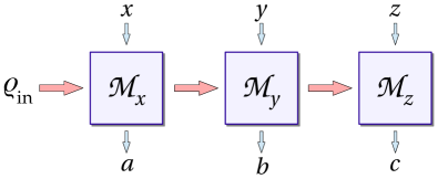
Figure 1: Schematic representation of the situation considered in this paper. A quantum system (described by a density matrix $\varrho_{\rm in}$) is subjected to a sequence of measurements, each of them drawn from the set of possible measurements $\{\mathcal{M}_{i}\}$. The choice of the measurements is denoted by $x,y,z,...$ and the result by $a,b,c,...$. This results in a probability distribution $p(abc...|xyz...)$. Note that if $x=y$ the measurement $\mathcal{M}_{x}$ is repeated two times, but this does not imply that the results $a$ and $b$ are the same.

It remains unclear how to obtain such bounds for more general classes of measurements, as allowed by quantum mechanics where the post-measurement state may depend on the measurement result and the input state in a non-trivial wayfootnote . This makes quantitative and analytical statements often difficult maurochsh .

In this paper we characterize temporal quantum correlations when measurements can be repeated, without making any assumption on the measurements. First, we study general correlations without assuming the formalism of quantum mechanics, the only restriction being that later measurements do not influence the previous ones. The resulting probabilities form a polytope and we characterize its extreme points. Then, we relate this to the quantum mechanical formalism. We prove that any possible temporal correlation can be generated from measurements on a quantum system, but the quantum system may be required to be high-dimensional. Interestingly, already for the simplest case of two measurements with two outcomes each, and measurement sequences of length two, there are temporal correlations which cannot originate from quantum measurements on a qubit. This is unexpected, as the standard correlation for this case based on the CHSH inequality fritz-temporal1 ; budroni does not have this property and all possible values for it can come from generalized measurements on a qubit budroni ; maurochsh . The correlations we found can then be used as tests of the quantum dimension: We provide analytical bounds without making any assumptions about the measurements and a violation of these proves that the tested quantum system is three-dimensional. Finally, we discuss a possible implementation using nitrogen-vacancy (NV) centers in diamond.

II The scenario

We consider temporal sequences of measurements on a quantum state $\varrho_{\rm in}$ (see Fig. 1). In the simplest scenario, we consider two possible measurements with two outcomes at two times. More precisely, at time $t_{1}$ one can choose between two different measurement settings $\mathcal{M}_{0}$ and $\mathcal{M}_{1}$. The input $x\in\{0,1\}$ determines which measurement is performed and the output is labelled by the variable $a\in\{0,1\}$. At a later time $t_{2}$, one can again choose between the two measurements $\mathcal{M}_{i}$, where the input is labelled by $y$ and the output by $b$. This leads to joint probabilities $p(ab|xy)$ for this measurement sequence. Note that for $x=y$ the same measurement is implemented at time $t_{1}$ and $t_{2}$, but different outcomes may be obtained. Clearly, the probabilities obey the conditions of positivity, $p(ab|xy)\geq 0$ and normalization, $\sum_{a,b}p(ab|xy)=1.$ In addition, the first measurement is not influenced by the second one, so the probabilities fulfill the arrow of time (AoT) constraints kofler

$$\sum_{b}p(ab|xy)=\sum_{b}p(ab|xy^{\prime})\quad\mbox{ for all }a,x,y,y^{\prime}.$$ (1)

This condition can be used to define the marginal probabilities $p(a|x)$ as

$$p\left(a|x\right):=\sum_{b}p\left(ab|xy\right)\quad\mbox{ for all }a,x,y.$$ (2)

It is easy to see that the set of all probabilities forms a polytope. Furthermore, the definition and constraints can straightforwardly be generalized to sequences of arbitrary length $L$, number of results per measurement $R$ and number of possible measurement settings $S$ per time step. Again for any $R,S$ and $L$, the AoT constraints define a polytope, the so-called temporal correlation polytope, labelled by $P_{L}^{R,S}$.

Before characterizing this polytope, let us review how the probabilities are determined in quantum mechanics. We consider the most general notion of measurements in quantum mechanics, which are described by quantum instruments (see, e.g., Ref. teiko ). A measurement setting $\mathcal{M}_{s}$ with the outcomes $\{r\}$ corresponds to a set of completely positive maps $\mathcal{I}_{r|s}$ which describe the state update and the probabilities. After measuring $\mathcal{M}_{s}$ on the state $\varrho_{\rm in}$ and finding the result $r$ the (not normalized) post-measurement state is given by

$$\varrho_{\rm out}=\mathcal{I}_{r|s}(\varrho_{\rm in}),$$ (3)

and the probabilities of obtaining the result is given by $p(r|s)={\rm tr}[\mathcal{I}_{r|s}(\varrho_{\rm in})].$ Since some result must occur, the maps $\mathcal{I}_{r|s}$ sum up to a trace-preserving map, $\sum_{r}\mathcal{I}_{r|s}=\Lambda_{s}.$ If one is interested in the probabilities only, one can obtain them also by effects $\mathcal{E}_{r|s}$. This means that for any measurement there are positive semidefinite operators $\mathcal{E}_{r|s}$ which sum up to the identity $\sum_{r}\mathcal{E}_{r|s}=\openone$ and which obey $p(r|s)={\rm tr}(\mathcal{E}_{r|s}\varrho_{\rm in})$. Finally, note that in our formalism we do not consider a possible time evolution of the quantum system between the measurements. If there is such a time evolution, it often can be absorbed in the positive maps $\mathcal{I}_{r|s}$, as it just changes the post-measurement state.

III Characterizing the polytope

Let us first mention a result on the structure of probability distributions $p(abc\dots|xyz\dots)$ that fulfill the AoT constraints.

Observation 1. A temporal probability distribution $p(abc\dots|xyz\dots)$ fulfills the AoT constraints if and only if it can be written as

$$p(abc\dots|xyz\dots)=p(a|x)p(b|axy)p(c|abxyz)\dots,$$ (4)

with $p\left(a|x\right)$, $p(b|axy)$, $p(c|abxyz)$ etc. being probability distributions with respect to the variables $a$, $b$, $c$ etc.

Note that this is a straightforward generalization of an observation made in Ref. fritz-temporal1 . To understand this, note that for sequences of length two where $p(ab|xy)$ is given, one can define $p(b|axy)=p(ab|xy)/p(a|xy)=p(ab|xy)/p(a|x)$ and find the decomposition. On the other hand, if $p(b|axy)$ and $p(a|x)$ are given, Eq. (4) defines $p(ab|xy)$ and one can directly verify all the desired properties. More details for longer sequences are given in Appendix A.

The extreme points of $P_{L}^{R,S}$, i.e. the maximally achievable correlations can then be characterized as follows:

Observation 2. The extreme points of the temporal correlation polytope $P_{L}^{R,S}$ are given by the deterministic assignments that fulfill the AoT constraints. Here, a deterministic assignment denotes a probability distribution that takes either the value $0$ or $1$.

This Observation has been made independently in Ref. jannik-thesis and Ref. abbott . We present the proof from Ref. jannik-thesis in Appendix A. Using the two observations, one can derive a simple equation to determine the number of extreme points $N_{L}^{R,S}$ for the polytopes $P_{L}^{R,S}$. We find

$$N^{R,S}_{L}=\prod_{i=0}^{L-1}(R^{S})^{(S^{i})}=(R^{S})^{(\frac{S^{L}-1}{S-1})}.$$ (5)

This formula can directly be understood for the simple case of $L=S=R=2$. To determine the number of extreme points of the polytope $P_{2}^{2,2}$, we first have to assign deterministic values for the marginal probabilities $p(a|x)$. For the probability distribution $p(a|x)$, there exist $R^{S}=2^{2}=4$ different deterministic assignments $p(a|x)=0,1$. For the probability distribution of the second measurement we have, for a given first measurement, $R^{S}=2^{2}=4$ different deterministic assignments, but there are $S^{1}=2$ possible first measurement settings. This results in $2^{2}\cdot(2^{2})^{2}=64$ extreme points for the polytope $P_{2}^{2,2}$. In general, Eq. (5) can be verified via induction and the geometric series, see also Appendix B.

IV Relation to quantum mechanics

Having characterized the structure and number of the extreme points of $P_{L}^{R,S}$, we will now clarify whether these extreme points can be reached by physical theories such as quantum mechanics.

For simplicity, let us focus on the polytope $P_{2}^{2,2}$. Quantum mechanics fulfills the AoT constraints. In particular, the probabilities factorize via

$$p(ab|xy) =p(a|x)p(b|axy)$$

$$={\rm tr}(\mathcal{E}_{a|x}\operatorname{\varrho}_{\rm in}){\rm tr}(\mathcal{E}_{b|y}\left[\frac{\mathcal{I}_{a|x}(\operatorname{\varrho}_{\rm in})}{{\rm tr}(\mathcal{E}_{a|x}\operatorname{\varrho}_{\rm in})}\right]).$$ (6)

As stated in the following theorem all temporal probability distributions can be reached with quantum mechanical measurements. Note that our result is different from a similar statement in Ref. fritz-temporal1 , as we assume that measurements can be repeated and therefore some measurements must be represented by the same instrument (applied at different times) in the quantum mechanical description.

Theorem 1. Any probability distribution of $P_{L}^{R,S}$ can be reached in quantum mechanics. The quantum mechanical representation may require a high-dimensional quantum system.
Proof. We consider the case of $P_{2}^{2,2}$, the construction can then be generalized to longer sequences. Let us first consider an extreme point. In order to reach this with measurements on a three-level system, i.e. a qutrit, we use the states $|0\rangle$, $|1\rangle$, and $|2\rangle$, where $|0\rangle$ is the initial state of the system, $|1\rangle$ is the post-measurement state after a first measurement with $x=0$ and $|2\rangle$ is the post-measurement after the first measurement $x=1$.

For writing down suitable effects, we denote by $a_{0}^{x}$ the (deterministic) outcome when measuring $x$ at the first time step, by $a_{1}^{y}$ the outcome for the measurement $y$ at the second time step if one had measured $x=0$ and $a_{2}^{y}$ denotes the outcome of the second measurement if one had measured $x=1$. Note that $x,y$ are just labels for the first and second measurement, which have the same range of values. We have to define measurements that can be carried out as a first and second measurement and denote the setting by $s$ and the result by $r$.

For each measurement $s\in\{0,1\}$ we define the set $\mathcal{P}_{s}$ which collects all the $i$ for which $a_{i}^{s}$ indicates a “$0$” result, i.e. $\mathcal{P}_{s}=\{i:a_{i}^{s}=0\}$. The effects of the measurements are then defined as $\mathcal{E}_{0|s}=\sum_{i\in\mathcal{P}_{s}}|i\rangle\!\langle i|$ and $\mathcal{E}_{1|s}=\openone-\mathcal{E}_{0|s}$. Note that with the initial and post-measurement states as defined before this ensures that the desired measurement outcomes are obtained. For writing down the complete instrument, we define $U_{0}=|0\rangle\langle 1|+|1\rangle\langle 0|+|2\rangle\langle 2|$ for the measurement $s=0$ and $U_{1}=|0\rangle\langle 2|+|2\rangle\langle 0|+|1\rangle\langle 1|$ for the measurement $s=1$, which will take care of the post-measurement states. That is we define the measurement operators $M_{r|s}=U_{s}\mathcal{E}_{r|s}$ and the corresponding instrument $\mathcal{I}_{r|s}(\varrho_{\rm in})=M_{r|s}\varrho_{\rm in}M_{r|s}^{\dagger}$. It can be easily seen that this reproduces the desired results if the system is initially prepared in $|0\rangle$.

For the extension to non-extreme probability distributions in $P_{2}^{2,2}$ note first that in the previous construction the state and the effects depend on the extreme vertex, so one cannot directly obtain mixtures in $P_{2}^{2,2}$ by mixing states and effects. But via increasing the dimension, it can be done as follows: Let ${E}$ be the set of all extreme points of the polytope $P_{2}^{2,2}$ and $\{|0_{e}\rangle,|1_{e}\rangle,|2_{e}\rangle\}_{e\in{E}}$ be the orthonormal vectors for the extreme vertex as constructed above. We also denote the measurement operators as $M_{r|s}^{e}$, stressing the dependence on the vertex $e\in E$. If we have a general set of probability distributions $\mathfrak{p}$ in $P_{2}^{2,2}$ we can write it as $\mathfrak{p}=\sum_{e}\alpha_{e}e$ with probabilities $\alpha_{e}$ and $e\in{E}$. Then, this can be reproduced by taking as an initial state the direct sum $\varrho=\bigoplus_{e\in{E}}\alpha_{e}|0_{e}\rangle\!\langle 0_{e}|$ and as measurement operators $M_{r|s}=\bigoplus_{e\in E}M_{r|s}^{e}.$ $\hfill\Box$

Note that the protocol that allows us to obtain any probability distribution in $P_{2}^{2,2}$ corresponds to a completely classical strategy as it does not require any coherences. It can be shown that for $R=S=2$ there exist extreme points which require a minimal dimension to be reached that scales at least as $2^{L+1}/L$ generaltempsequ .

V Temporal correlations for a qubit

The previous construction allows us to reach all extreme points of the polytope $P^{2,2}_{2}$ using a three-level quantum system. However, already in the simple scenario of $P^{2,2}_{2}$ not all extreme points can be reached using a qubit only. Among the 64 extreme vertices many are equivalent, as one can relabel the measurement settings $0\leftrightarrow 1$ and the measurement outcomes $0\leftrightarrow 1$ footnote2 . Taking these symmetries into account, 10 extreme vertices remain, and 6 of these can be reached via measurements on a qubit in a simple manner jannik-thesis . The four remaining extreme points are

$$e_{1}:\;p(00|00)=p(00|11)=p(01|01)=p(01|10)=1,$$

$$e_{2}:\;p(01|00)=p(01|11)=p(00|01)=p(00|10)=1,$$

$$e_{3}:\;p(01|00)=p(00|11)=p(01|01)=p(01|10)=1,$$

$$e_{4}:\;p(01|00)=p(01|11)=p(01|01)=p(00|10)=1.$$ (7)

It is instructive to discuss these vertices in a qualitative manner, leading to an intuitive understanding why they cannot be reached by measurements on a qubit. Let us first discuss the vertex $e_{1}$. From $p(01|01)=p(01|10)=1$ it follows that the measurements $\mathcal{M}_{0}$ and $\mathcal{M}_{1}$ cannot be trivial in the sense that their result must depend on the input state. Then, the probabilities $p(00|00)=p(00|11)=1$ can only be reached on a qubit if the effects of the measurements $\mathcal{M}_{0}$ and $\mathcal{M}_{1}$ are of the form $\mathcal{E}_{0|i}=|a_{0}\rangle\!\langle a_{0}|+p_{i}|a_{1}\rangle\!\langle a_{1}|$ and $\mathcal{E}_{1|i}=(1-p_{i})|a_{1}\rangle\!\langle a_{1}|$ with $0\leq p_{i}<1$ and $\{|a_{0}\rangle,|a_{1}\rangle\}$ being an orthonormal basis and the input state is $|a_{0}\rangle$. Moreover, it follows that the measurements do not disturb this input state. But then, a contradiction to $p(01|01)=p(01|10)=1$ occurs.

Concerning the vertex $e_{3}$, as already mentioned the fact that $p(01|01)=p(01|10)=1$ implies that the outcome of $\mathcal{M}_{1}$ (and $\mathcal{M}_{0}$) has to depend on the state on which the measurement is performed. It follows then from $p(00|11)=1$ that $\mathcal{M}_{1}$ has effects of the form $\mathcal{E}_{0|1}=|a_{0}\rangle\!\langle a_{0}|+p_{1}|a_{1}\rangle\!\langle a_{1}|$ and $\mathcal{E}_{1|1}=(1-p_{1})|a_{1}\rangle\!\langle a_{1}|$ with $0\leq p_{1}<1$ and the input state is $|a_{0}\rangle$ which remains unchanged by measuring $\mathcal{M}_{1}$. However, considering $p(01|00)=p(01|10)=1$ this leads to a contradiction. The discussion of the vertices $e_{2}$ and $e_{4}$ is similar, further details and rigorous proofs can be found in Appendix D.

VI Dimension witnesses

The fact that the vertices can not be represented by qubit systems can be made quantitative by characterizing the amount to which they can be approximated. For that we consider two expressions, derived from the vertices $e_{1}$ and $e_{3}$,

$$\operatorname{\mathcal{B}}_{1}=p(00|00)+p(00|11)+p(01|01)+p(01|10),$$

$$\operatorname{\mathcal{B}}_{3}=p(01|00)+p(00|11)+p(01|01)+p(01|10).$$ (8)

For these expectation values we can state:

Theorem 2. For arbitrary measurements on a qubit the following bounds hold:

$$\operatorname{\mathcal{B}}_{1} \leq\mathcal{C}_{1}=3,$$

$$\operatorname{\mathcal{B}}_{3} \leq\mathcal{C}_{3}\approx 3.186.$$ (9)

The bound $\mathcal{C}_{3}$ is given by the root of a polynomial of degree ten.

Proof. The proof is given in Appendix C.

The first question that arises is whether similar bounds can be established for the vertices $e_{2}$ and $e_{4}$. We first note that the structure of the vertices $e_{1}$ and $e_{2}$ is similar and that the same holds true for the vertices $e_{3}$ and $e_{4}$. For the vertices $e_{2}$ and $e_{4}$ one can analytically reduce the problem of finding the maximal expectation value for the corresponding $\operatorname{\mathcal{B}}_{2}$ and $\operatorname{\mathcal{B}}_{4}$, to a maximization that depends only on two parameters. Performing the remaining maximization numerically suggests that $\operatorname{\mathcal{B}}_{2}$ is upper bounded by $\mathcal{C}_{1}$ and $\operatorname{\mathcal{B}}_{4}$ is upper bounded by $\mathcal{C}_{3}$. This reflects the similarity among the pairs of vertices mentioned above. For the vertex $e_{4}$ one can further analytically show that $\operatorname{\mathcal{B}}_{4}$ is upper bounded by $2+\sqrt{2}$.

It is instructive to characterize the qubit measurements giving the maximal value for $\operatorname{\mathcal{B}}_{1}$ and $\operatorname{\mathcal{B}}_{3}.$ For $\operatorname{\mathcal{B}}_{1}$ the optimal measurement $\mathcal{M}_{0}$ is a trivial measurement, giving always the result $0$. Then, if $\mathcal{M}_{1}$ is a $\sigma_{z}$ measurement, the initial state is $|0\rangle$ and $\mathcal{M}_{0}$, although giving a fixed result, flips the state, a value of $\operatorname{\mathcal{B}}_{1}=3$ can be reached. For $\operatorname{\mathcal{B}}_{3}$ the optimal measurements can be shown to have projective effects. It should be noted that for such measurements $\operatorname{\mathcal{B}}_{3}$ is equivalent to $\operatorname{\mathcal{B}}_{4}$. Note further that from the proof of Theorem 1 it follows that $\operatorname{\mathcal{B}}_{1}=\operatorname{\mathcal{B}}_{3}=4$ can be reached on a three-level system.

Finally, the preceding Theorem shows that temporal correlations can be used for characterizing the dimension of quantum systems in a device-independent manner. Namely, if one of the inequalities in Theorem 2 is violated, one knows that the underlying system is not a qubit, without assuming anything about the measurements or the state transformations between the measurements footnote3 . So far, dimension tests have been proposed using Bell inequalities brunner , prepare & measure schemes gallego or more general input-output correlations dallarno1 ; dallarno2 , the time evolution of the expectation value of a single observable wolf or temporal correlations and contextuality guehnedim ; fritz-temporal1 ; budroni-emary . The schemes using Bell inequalities cannot be used with a single qutrit and moreover, recently it turned out that their violation can also be observed with pairs of qubit systems cong ; tristan . The approach in Ref. dallarno1 , based on a result on noiseless $n$-level quantum channels frenkel , is, however, restricted to some specific channels, which are inserted between the preparation and the measurement. In Ref. dallarno2 , the results are not limited to specific measurement, but they are restricted to the qubit case. Such approaches have been further developed to propose a principle, based on temporal correlations, that may single out quantum theory among generalized probabilistic theories dallarno3 , and to provide a characterization of quantum memories based on temporal correlations rosset . The existing proposals using temporal correlations guehnedim ; fritz-temporal1 ; budroni-emary make assumptions about the nature of the measurements, e.g., they have to be projective. The dimension bound derived in wolf is based on the expectation values of a single observable evaluated after $t$ uses of a quantum channel and assumes that the time evolution is Markovian and homogeneous in time.

The dimension witness from Theorem 2 is closest to the prepare & measure scheme from Ref. gallego , which is also device-independent. As any measurement can be viewed as a state preparation, our scheme may also be interpreted as prepare & measure scheme, but there are several advantages of our approach: First, the bound for $\operatorname{\mathcal{B}}_{1}$ leads to larger separation among qutrits and qubits than some of the inequalities in Ref. gallego . Second, our approach can be generalized to measurement sequences of length three or longer, and then an interpretation as a prepare & measure scheme is not possible anymore.

Our scheme does not only provide a distinction between a qubit and higher-dimensional systems but also allows us to establish a lower bound on the distance between the measured system and a qubit. In order to quantify this distance one may define $(d+\epsilon)$-dimensional systems as systems for which the initial states as well as all possible post-measurement states of the instruments deviate only by $\epsilon$ from the same d-dimensional subspace. More precisely, a $(d+\epsilon)$- system is given by an initial state $\operatorname{\varrho}_{\rm in}$ and instruments $\{\mathcal{I}_{a|x}\}_{a}$ with the property that there exists a projector on a d-dimensional subspace, $P_{d}$, such that $\lVert P_{d}\operatorname{\varrho}_{\rm in}P_{d}-\operatorname{\varrho}_{\rm in}\rVert_{\rm tr}\leq\epsilon$ and for all $a,x$ and quantum states $\rho$ it holds that $\lVert P_{d}\mathcal{I}_{a|x}(\rho)P_{d}-\mathcal{I}_{a|x}(\rho)\rVert_{\rm tr}\leq\epsilon$. It can be shown that for $(2+\epsilon)$-dimensional systems it holds that $\mathcal{B}_{i}\leq C_{i}+12\epsilon$ (see Appendix D). Hence, from the value of $\mathcal{B}_{i}$ determined in an experiment it is possible to deduce a lower bound on $\epsilon$.

VII Possible implementation with NV centers

NV centers are well-characterized quantum systems nv-general and, since they contain several energy levels, they are candidates for testing the inequalities derived above.

The relevant energy levels of an NV cente are a ground state manifold ³A and a set of excited states ³E. Both manifolds consist of three states, corresponding to the $m_{s}=0$ and $m_{s}=\pm 1$ quantum numbers. The ground state manifold can be used as a qutrit: In the presence of a magnetic field they are non-degenerate and at low temperatures microwave fields can be used to drive unitary transitions between the three states. Coupling the ground state manifold ³A to the manifold ³E with resonant excitation preserves the value of $m_{s}$, but as the $m_{s}=\pm 1$ state in ³E decays with some probability to the $m_{s}=0$ state in ³A, the ground state manifold can be prepared in the state $m_{s}=0$ with high fidelity robledo . By driving the transition from $m_{s}=0$ in ³A to $m_{s}=0$ in ³E only, and detecting fluorescence, the $m_{s}=0$ state can be read out and at low temperatures the $m_{s}=\pm 1$ states remain unaffected robledo .

Our procedure of reaching the extreme vertex $e_{1}$ using a three-level system (see the proof of Theorem 1) leads to the following operators: Initially, the NV center is prepared in the $|0\rangle=|m_{s}=0\rangle$ state. The measurement $\mathcal{M}_{0}$ is performed in the following way: First, the NV center is measured projectively in the $|2\rangle=|m_{s}=-1\rangle$ state (result “1”) or in the orthogonal subspace, spanned by $|0\rangle$ and $|1\rangle=|m_{s}=1\rangle$ (result “0”). This first step can be achieved by first applying a unitary transformation, then performing the projective measurement of $|0\rangle$ and finally undoing the unitary again. The second step of the measurement $\mathcal{M}_{0}$ is a unitary transformation $U_{0}=|0\rangle\langle 1|+|1\rangle\langle 0|+|2\rangle\langle 2|$ independent of the measurement result. The measurement $\mathcal{M}_{1}$ is implemented similarly, first one projects onto $|1\rangle$ (result “1”) or the orthogonal subspace (result “0”) and finally one performs $U_{1}=|0\rangle\langle 2|+|2\rangle\langle 0|+|1\rangle\langle 1|.$ These measurements will lead to $\operatorname{\mathcal{B}}_{1}=4$ which is the maximal violation of the inequality $\operatorname{\mathcal{B}}_{1}\leq 3.$

VIII Conclusion

We have characterized general temporal correlations coming from sequences of measurements on a quantum system. We first considered general correlations obeying the arrow-of-time condition and showed that all of these can be attained by quantum mechanics. If the dimension of the quantum system is restricted, however, not all correlations can arise from quantum mechanical systems. This allows us to construct dimension witnesses, which can be implemented with NV centers in diamond.

There are several directions in which our approach can be generalized. First, it would be interesting to characterize the set of quantum correlations coming from a fixed dimension further. To give an example of an open question, it is not clear whether this set it convex. Second, it is promising to consider longer measurement sequences for dimension tests. This will probably lead to higher violations and easier experimental implementation. Finally, it is important to understand the classical protocols to generate temporal correlations. For instance, classical systems with a bounded memory can also not reproduce all temporal correlations, and this may help to characterize the quantum advantage in information processing based on sequential measurements.

We thank Johannes Greiner, Matthias Kleinmann and Gael Sentís for discussions. This work was supported by the DFG, the Austrian Science Fund (FWF): M 2107 (Meitner-Programm) and the ERC (Consolidator Grant No. 683107/TempoQ).

IX Appendix A: Proof of the Observations 1 and 2

In this part of the Appendix, we will present the proofs of Observations 1 and 2. We start with the proof of Observation 1 which we will use afterwards to prove Observation 2.

Observation 1. A temporal probability distribution $p(abc\dots|xyz\dots)$ fulfills the AoT constraints if and only if it can be written as

$$p(abc\dots|xyz\dots)=p(a|x)p(b|axy)p(c|abxyz)\dots,$$ (10)

with $p\left(a|x\right)$, $p(b|axy)$, $p(c|abxyz)$ etc. being probability distributions with respect to the variables $a$, $b$, $c$ etc.

Proof. We will prove this Observation for the case $L=3$, as it is straightforward to generalize the proof to sequences of arbitrary length. First, assume that the probability distribution $p(abc|xyz)$ fulfills the AoT constraints. In this case, the marginal probabilities $p(a|x)$ are well defined. We will further introduce two conditional probabilities $p(b|axy)$ and $p(c|abxyz)$. We define $p(b|axy)$ as

$$p\left(b|axy\right):=\dfrac{p\left(ab|xy\right)}{\sum_{b}p\left(ab|xy\right)}=\dfrac{p\left(ab|xy\right)}{p\left(a|x\right)},$$ (11)

for $p\left(a|x\right)\neq 0$, and one can, for example, choose

$$p\left(b|axy\right):=0,$$ (12)

for $p\left(a|x\right)=0$. It is easy to see that $p(b|axy)$ is a valid probability distribution, if $p(a|x)\neq 0$. First $p(b|axy)$ is positive since $p(ab|xy)$ and $p(a|x)$ are positive and second we have

$$\sum_{b}p(b|axy)=\dfrac{\sum_{b}p(ab|xy)}{p(a|x)}=1.$$ (13)

The conditional probability $p(c|abxyz)$ is defined as

$$p(c|abxyz)=\dfrac{p(abc|xyz)}{p(ab|xy)},$$ (14)

if $p(ab|xy)\neq 0$ and can be chosen to be zero otherwise. In an analogous way as for $p(b|axy)$, we can show that $p(c|abxyz)$ is a valid probability distribution if $p(ab|xy)\neq 0$. We then simply have

$$p\left(abc|xyz\right) =p\left(a|x\right)\dfrac{p\left(ab|xy\right)}{p\left(a|x\right)}\dfrac{p\left(abc|xyz\right)}{p\left(ab|xy\right)}$$

$$=p\left(a|x\right)p\left(b|axy\right)p\left(c|abxyz\right).$$ (15)

Hence the probability distribution $p(abc|xyz)$ can be factorized if it fulfills the AoT constraints.

Now assume that we have probability distributions $p(a|x)$, $p(b|axy)$ and $p(c|abxyz)$. The product of these probabilities

$$p(a|x)p(b|axy)p(c|abxyz)=:p(abc|xyz),$$ (16)

fulfills the AoT constraints, as

$$\sum_{b,c}p\left(abc|xyz\right) =\sum_{b,c}p\left(a|x\right)p\left(b|axy\right)p\left(c|abxyz\right)$$

$$=p\left(a|x\right)\sum_{b}p\left(b|axy\right)\sum_{c}p\left(c|abxyz\right)$$

$$=p\left(a|x\right)\quad\forall a,x,y,z,$$ (17)

and

$$\sum_{c}p\left(abc|xyz\right) =\sum_{c}p\left(a|x\right)p\left(b|axy\right)p\left(c|abxyz\right)$$

$$=p\left(a|x\right)p\left(b|axy\right)\sum_{c}p(c|abxyz)$$

$$=p\left(a|x\right)p\left(b|axy\right)$$

$$=:p\left(ab|xy\right)\quad\forall a,b,x,y,z.$$ (18)

So the probability distribution $p\left(abc|xyz\right)=p\left(a|x\right)p\left(b|axy\right)p\left(c|abxyz\right)$ fulfills the AoT constraints, which completes the proof. $\hfill\Box$

Using Observation 1, we can now prove Observation 2:

Observation 2. The extreme points of the temporal correlation polytope $P_{L}^{R,S}$ are given by the deterministic assignments that fulfill the AoT constraints. Here, a deterministic assignment denotes a probability distribution that takes either the value $0$ or $1$.

Proof. We need to show that

• All deterministic assignments are extreme

• Every vector $v$ consisting of the probabilities $p(abc...|xyz...)$ can be written as a convex combination of the vectors corresponding to deterministic assignments.

The proof of (i) is trivial in the sense that a deterministic assignment for the vector $v$ can never be written as a convex combination of other vectors. We will show (ii) for the polytope $P_{2}^{2,2}$, however, one can easily generalize the method to an arbitrary polytope $P_{L}^{R,S}$.

Let us first consider the probabilities $p(a|x)$ for fixed $x$. Let us define the vector

$$v_{x} =\left(\begin{array}[]{c}p(0|x)\\ p(1|x)\end{array}\right)=c\left(\begin{array}[]{c}1\\ 0\end{array}\right)+(1-c)\left(\begin{array}[]{c}0\\ 1\end{array}\right)=\left(\begin{array}[]{c}c\\ 1-c\end{array}\right),$$ (27)

which is a convex combination of $(1,0)^{T}$ and $(0,1)^{T}$, describing probability $1$ for outcome $0$ and probability $1$ for outcome $1$, respectively.

Let us assume first that $c\neq 0,1$. Then, for fixed $x$ and $y$, the vector containing the conditional probabilities $p(b|axy)$ can also be written as a convex combination. In this case, we define the vector

$$v_{xy} =\left(\begin{array}[]{c}p(0|0xy)\\ p(1|0xy)\\ p(0|1xy)\\ p(1|1xy)\end{array}\right)=d\left(\begin{array}[]{c}1\\ 0\\ 0\\ 0\end{array}\right)+(1-d)\left(\begin{array}[]{c}0\\ 1\\ 0\\ 0\end{array}\right)$$ (40)

$$+e\left(\begin{array}[]{c}0\\ 0\\ 1\\ 0\end{array}\right)+(1-e)\left(\begin{array}[]{c}0\\ 0\\ 0\\ 1\end{array}\right)=\left(\begin{array}[]{c}d\\ 1-d\\ e\\ 1-e\end{array}\right).$$ (53)

The first two entries describe the probability distribution for $a=0$, with the convex coefficient $d$ and the last two, the probability distribution for $a=1$ with the convex coefficient $e$. Both convex combinations are independent of each other.

We now want to show that for fixed $x$ and $y$ the probability distribution $p(ab|xy)$ is always a convex combination if the conditional probabilities are non-deterministic. For this, let us define the vector

$$v=\left(\begin{array}[]{c}p(00|xy)\\ p(01|xy)\\ p(10|xy\\ p(11|xy)\end{array}\right)=\left(\begin{array}[]{c}p(0|x)p(0|0xy)\\ p(0|x)p(1|0xy)\\ p(1|x)p(0|1xy\\ p(1|x)p(1|1xy)\end{array}\right),$$ (54)

where we used the fact that due to Observation 1, we can factorize the probabilities $p(ab|xy)$ into the conditional probabilities $p(a|x)$ and $p(b|axy)$. If we replace the probabilities $p(a|x)$ and $p(b|axy)$ with the respective coefficients in the vectors in Eqs. (27) and (40), we obtain

$$\small v =\left(\begin{array}[]{c}cd\\ c(1-d)\\ (1-c)e\\ (1-c)(1-e)\end{array}\right)=cd\left(\begin{array}[]{c}1\\ 0\\ 0\\ 0\end{array}\right)+c(1-d)\left(\begin{array}[]{c}0\\ 1\\ 0\\ 0\end{array}\right)$$ (67)

$$+(1-c)e\left(\begin{array}[]{c}0\\ 0\\ 1\\ 0\end{array}\right)+(1-c)(1-e)\left(\begin{array}[]{c}0\\ 0\\ 0\\ 1\end{array}\right),$$ (76)

which is a convex combination of at least two different vectors if $0<c<1$, $0\leq d\leq 1$ and $0\leq e\leq 1$, since $cd,c(1-d),(1-c)e,(1-c)(1-e)\geq 0$ and $cd+c(1-d)+(1-c)e+(1-c)(1-e)=1$.

Up to now, we restricted ourselves to the case, where $p(a|x)\neq 0$ for all $a$, given $x$. Consider next the case of a deterministic assignment for $p(a|x)$ and fixed $x$, i.e. $c=0$ or $c=1$. Assume without loss of generality that $c=1$. The vector $v$ is then of the form

$$v=\left(\begin{array}[]{c}d\\ (1-d)\\ 0\\ 0\end{array}\right)=d\left(\begin{array}[]{c}1\\ 0\\ 0\\ 0\end{array}\right)+(1-d)\left(\begin{array}[]{c}0\\ 1\\ 0\\ 0\end{array}\right),$$ (77)

which is still a convex combination of deterministic assignments.

Since we can construct vectors like this for every choice of $x$ and $y$, we find that all non-deterministic assignments for the vector $v$ are convex combinations of deterministic assignments. $\hfill\Box$

X Appendix B: On the number of extreme vertices

In this part of the Appendix, we will present the proof of Eq. (5), which quantifies the number of extreme points of $P_{L}^{R,S}$.

We prove this equation by induction. For sequences of length $L=1$, we have $R^{S}$ different possibilities to assign a deterministic value to the probabilities $p(a|x)$, i.e $N_{1}^{R,S}=\prod_{i=0}^{0}(R^{S})^{(S^{i})}=R^{S}.$

Next we show that the equation is true for a sequence of length $L+1$, under the assumption that it is valid for sequences of length $L$. Given a specific sequence of measurements of length $L$ there are $R^{S}$ different deterministic assignments possible for the probability distribution of the measurements at time $L+1$. Moreover, the number of possible measurement settings for a sequence of length $L$ is given by $S^{L}$. This leads to $(R^{S})^{S^{l}}$ different possible deterministic assignments for the probability distributions of the measurements at time $L+1$ of an extreme point. Hence, the total number of different deterministic assignments for sequences of length $L+1$ is given by $N_{L}^{R,S}\cdot(R^{S})^{S^{L}}=N_{L+1}^{R,S}$. With this we have shown that

$$N^{R,S}_{L}=\prod_{i=0}^{L-1}(R^{S})^{(S^{i})}=(R^{S})^{(\frac{S^{L}-1}{S-1})},$$ (78)

where for the second equality the well known formula for the partial sum of the geometric series has been used. $\hfill\Box$

XI Appendix C: Proof of Theorem 2

This part of the appendix is concerned with the proof of Theorem 2. As mentioned in the main text, there are four (up to relabeling of the measurement outcomes and settings) extreme points of $P_{2}^{2,2}$ that cannot be reached via measurements on a qubit:

$$e_{1}:\;p(00|00)=p(00|11)=p(01|01)=p(01|10)=1,$$

$$e_{2}:\;p(01|00)=p(01|11)=p(00|01)=p(00|10)=1,$$

$$e_{3}:\;p(01|00)=p(00|11)=p(01|01)=p(01|10)=1,$$

$$e_{4}:\;p(01|00)=p(01|11)=p(01|01)=p(00|10)=1.$$ (79)

In order to quantify to which amount they can be approximated we introduced in the main text the quantities

$$\operatorname{\mathcal{B}}_{1}=p(00|00)+p(00|11)+p(01|01)+p(01|10),$$

$$\operatorname{\mathcal{B}}_{3}=p(01|00)+p(00|11)+p(01|01)+p(01|10),$$ (80)

for which one can can find upper bounds for two-dimensional systems as stated in Theorem 2:

Theorem 2. For arbitrary measurements on a qubit the following bounds hold:

$$\operatorname{\mathcal{B}}_{1} \leq\mathcal{C}_{1}=3,$$

$$\operatorname{\mathcal{B}}_{3} \leq\mathcal{C}_{3}\approx 3.186.$$ (81)

The bound $\mathcal{C}_{3}$ is given by the root of a polynomial of degree ten.

In the following subsections we will discuss the inequalities associated to the extreme points in more detail and provide a proof of Theorem 2.

XI.0.1 The extreme point $e_{1}$ and its associated temporal inequality

In this subsection we show that for arbitrary measurements on a single qubit the quantity $\operatorname{\mathcal{B}}_{1}=p(00|00)+p(00|11)+p(01|01)+p(01|10)$ is smaller or equal to $3$. Moreover, we show that this bound is tight, i.e. there exists a sequence of measurements on a qubit that allows to reach this value.

Proof. We will first show that for all initial states and post-measurement states the maximal value of $\operatorname{\mathcal{B}}_{1}$ is either smaller or equal to 3 [case (a)] or is attained in case the effects for both measurements are projectors [case (b)]. We will then consider case (b). We will identify the optimal initial and post-measurement states for such measurements and show that the maximal value for $\operatorname{\mathcal{B}}_{1}$ that can be obtained with projective effects is given by $3/2+\sqrt{2}<3$. We finally show that the upper bound given by $3$ is tight by providing an explicit protocol that allows to reach $\operatorname{\mathcal{B}}_{1}=3$.

Let us start by defining our notation. Throughout this proof the effects for $\mathcal{M}_{0}$ ($\mathcal{M}_{1}$) corresponding to the outcome $r\in\{0,1\}$ will be denoted by $\mathcal{E}_{r|0}$ ($\mathcal{E}_{r|1}$) respectively. We will first use the the following decomposition for these effects,

$$\mathcal{E}_{0|0}=a_{0}(\openone+b_{0}\,\vec{c}\cdot\vec{\sigma}),$$ (82)

$$\mathcal{E}_{1|0}=\openone-\mathcal{E}_{0|0},$$ (83)

$$\mathcal{E}_{0|1}=a_{1}(\openone+b_{1}\,\vec{d}\cdot\vec{\sigma}),$$ (84)

$$\mathcal{E}_{1|1}=\openone-\mathcal{E}_{0|1},$$ (85)

where $\vec{c},\vec{d}\in\mathbb{R}^{3}$, $|\vec{c}|=|\vec{d}|=1$ and $\vec{\sigma}=(\sigma_{1},\sigma_{2},\sigma_{3})$ with $\sigma_{i}$ being the Pauli matrices. Moreover, we choose without loss of generality that $b_{s}\geq 0$ and therefore due to $\openone\geq\mathcal{E}_{r|s}\geq 0$ we have that $0\leq a_{s}\leq\frac{1}{1+b_{s}}$ and $b_{s}\leq 1$ for $s\in\{0,1\}$. Note that due to the AoT constraints we have that $p(ab|xy)=p(a|x)p(b|axy)$ and therefore

$$\operatorname{\mathcal{B}}_{1} =p(0|0)[p(0|000)+p(1|001)]$$ (86)

$$+p(0|1)[p(1|010)+p(0|011)].$$

In the following we will denote by $\operatorname{\varrho}_{\rm in}$ the initial state and by $\operatorname{\varrho}_{x}$ the post-measurement states given that measurement $\mathcal{M}_{x}$ has been performed at time $t_{1}$ and outcome $0$ has been obtained. We will use for these states their Bloch decomposition

$$\operatorname{\varrho}_{j}=\frac{1}{2}(\openone+\vec{\alpha}_{j}\cdot\vec{\sigma})$$ (87)

for $j\in\{{\rm in},0,1\}$ where $\vec{\alpha}_{j}\in\mathbb{R}^{3}$. Note due to the fact that $\operatorname{\varrho}_{j}$ has to be positive semidefinite we have that $|\vec{\alpha}_{j}|\leq 1$. Using the decomposition for the effects in Eqs.(82)-(85) one obtains that

$$p(0|0)=a_{0}\,(1+b_{0}\vec{c}\cdot\vec{\alpha}_{\rm in}),$$ (88)

$$p(0|1)=a_{1}\,(1+b_{1}\vec{d}\cdot\vec{\alpha}_{\rm in}),$$ (89)

$$p(0|000)=a_{0}\,(1+b_{0}\vec{c}\cdot\vec{\alpha}_{0}),$$ (90)

$$p(1|001)=1-a_{1}\,(1+b_{1}\vec{d}\cdot\vec{\alpha}_{0}),$$ (91)

$$p(1|010)=1-a_{0}\,(1+b_{0}\vec{c}\cdot\vec{\alpha}_{1}),$$ (92)

$$p(0|011)=a_{1}\,(1+b_{1}\vec{d}\cdot\vec{\alpha}_{1}).$$ (93)

We will first show that for any $\operatorname{\varrho}_{\rm in}$, $\operatorname{\varrho}_{0}$, $\operatorname{\varrho}_{1}$ the maximum of $\operatorname{\mathcal{B}}_{1}$ is smaller or equal to 3 or is attained for $a_{0}=\frac{1}{1+b_{0}}$. In order to do so we first consider $\operatorname{\mathcal{B}}_{1}$ as a function of $a_{0}$ (all other parameters are assumed to be fixed but arbitrary) and derive its critical points. The derivative of $\operatorname{\mathcal{B}}_{1}$ with respect to $a_{0}$ is given by

$$\frac{d\operatorname{\mathcal{B}}_{1}}{da_{0}} =[p(0|000)+p(1|001)]\,(1+b_{0}\vec{c}\cdot\vec{\alpha}_{\rm in})$$

$$+p(0|0)\,(1+b_{0}\vec{c}\cdot\vec{\alpha}_{0})-p(0|1)\,(1+b_{0}\vec{c}\cdot\vec{\alpha}_{1}).$$ (94)

Multiplying this equation by $a_{0}$, one obtains at the critical points that

$$[p(0|000)+p(1|001)]p(0|0)$$

$$=p(0|1)[1-p(1|010)]-p(0|0)p(0|000)\leq 1.$$ (95)

Note that this implies that $\operatorname{\mathcal{B}}_{1}$ at the points where the derivative vanishes cannot exceed 3. We also have to consider the boundary of the domain for $a_{0}$, i.e. we have to consider $a_{0}=0$ and $a_{0}=\frac{1}{1+b_{0}}$. As can be easily seen $\operatorname{\mathcal{B}}_{1}\leq 2$ for $a_{0}=0$. In order to investigate the case $a_{0}=\frac{1}{1+b_{0}}$ in more detail we will use that in this case the effects of the measurements in Eqs.(82) and (83) can equivalently (by substituting $b_{0}=\frac{p}{2-p}$) be written as

$$\mathcal{E}_{0|0}=\frac{1}{2}[(2-p)\openone+p\,\vec{c}\cdot\vec{\sigma}],$$ (96)

$$\mathcal{E}_{1|0}=\frac{p}{2}(\openone-\,\vec{c}\cdot\vec{\sigma}),$$ (97)

where $0\leq p\leq 1$. Considering now $\operatorname{\mathcal{B}}_{1}$ as a function of $p$ (and again assuming all other parameters as fixed but arbitrary) one obtains for its derivative

$$\frac{d\operatorname{\mathcal{B}}_{1}}{dp} =-[p(0|000)+p(1|001)]\,\frac{1}{2}(1-\vec{c}\cdot\vec{\alpha}_{\rm in})$$

$$-p(0|0)\,\frac{1}{2}(1-\vec{c}\cdot\vec{\alpha}_{0})+p(0|1)\,\frac{1}{2}(1-\vec{c}\cdot\vec{\alpha}_{1}).$$ (98)

Hence, at the critical points we have that

$$0 =[p(0|000)+p(1|001)][p(0|0)-1]$$

$$+p(0|0)[p(0|000)-1]+p(0|1)p(1|010)$$

$$\geq 2[p(0|0)-1]+p(0|0)[p(0|000)-1]$$

$$+p(0|1)p(1|010),$$ (99)

where we used that $p(0|000)+p(1|001)\leq 2$ and $p(0|0)-1\leq 0$. This implies that

$$2 \geq p(0|0)[p(0|000)+1]+p(0|1)p(1|010)$$

$$\geq p(0|0)[p(0|000)+p(1|001)]+p(0|1)p(1|010)$$ (100)

and therefore it holds that $\operatorname{\mathcal{B}}_{1}\leq 3$ at the points where this derivative vanishes. We will next consider the boundary of the domain of $0\leq p\leq 1$. It is straightforward to see that for $p=0$ one obtains that $\operatorname{\mathcal{B}}_{1}\leq 3$. Before we investigate the case $p=1$ in more detail we will use that $\operatorname{\mathcal{B}}_{1}$ is invariant under exchanging measurement $0$ and measurement $1$. Therefore, one can analogously show that if the effects of measurement $1$ are not projectors we have that $\operatorname{\mathcal{B}}_{1}\leq 3$ and it only remains to show that in the case of projective effects for both measurements it also holds true that $\operatorname{\mathcal{B}}_{1}\leq 3$. In the following we we will use the notation

$$\mathcal{E}_{0|1}=\frac{1}{2}(\openone+\,\vec{d}\cdot\vec{\sigma}),$$ (101)

$$\mathcal{E}_{1|1}=\frac{1}{2}(\openone-\vec{d}\cdot\vec{\sigma}).$$ (102)

With this, Eq. (87) and Eqs. (96)-(97) for $p=1$ we have that $\operatorname{\mathcal{B}}_{1}$ is of the following form

$$\operatorname{\mathcal{B}}_{1} =\frac{1}{4}(1+\,\vec{c}\cdot\vec{\alpha}_{\rm in})[2+(\vec{c}-\vec{d})\cdot\vec{\alpha}_{0}]$$

$$+\frac{1}{4}(1+\vec{d}\cdot\vec{\alpha}_{\rm in})[2+(\vec{d}-\vec{c})\cdot\vec{\alpha}_{1}].$$ (103)

As $\frac{1}{2}(1+\,\vec{c}\cdot\vec{\alpha}_{\rm in})=p(0|0)\geq 0$ the optimal choice of $\vec{\alpha}_{0}$ is given by

$$\vec{\alpha}_{0}=\frac{\vec{c}-\vec{d}}{\sqrt{2-2\cos(\gamma)}}\,\,\mathrm{if}\,\,\vec{c}\neq\vec{d},$$ (104)

where here and in the following we will use the notation $\vec{c}\cdot\vec{d}=\cos(\gamma)$. Note that if both measurements have the same (projective) effects, i.e. $\vec{c}=\vec{d}$, $\operatorname{\mathcal{B}}_{1}$ is independent of $\operatorname{\varrho}_{0}$ and hence we do not have to specify $\operatorname{\varrho}_{0}$ in this case. Analogusly, $\operatorname{\mathcal{B}}_{1}$ is maximized by choosing

$$\vec{\alpha}_{1}=\frac{\vec{d}-\vec{c}}{\sqrt{2-2\cos(\gamma)}}\,\,\mathrm{if}\,\,\vec{c}\neq\vec{d}.$$ (105)

As before, $\operatorname{\mathcal{B}}_{1}$ is independent of $\operatorname{\varrho}_{1}$ in case $\vec{d}=\vec{c}$. Inserting the optimal choice of $\operatorname{\varrho}_{0}$ and $\operatorname{\varrho}_{1}$ in Eq.(103) and using the notation $X=2+\sqrt{2-2\cos(\gamma)}$ we obtain

$$\frac{X}{4}[2+(\vec{c}+\vec{d})\cdot\vec{\alpha}_{\rm in}].$$ (106)

Hence, the optimal choice of $\operatorname{\varrho}_{\rm in}$ is given by

$$\vec{\alpha}_{\rm in}=\frac{\vec{c}+\vec{d}}{\sqrt{2+2\cos(\gamma)}}\,\,\textrm{if}\,\,\vec{c}\neq-\vec{d}.$$ (107)

Similarly to before, we do not have to specify the input state if $\vec{c}=-\vec{d}$. Note that the optimal input and post-measurement states are all pure, i.e. $|\vec{\alpha}_{i}|=1$ for $i\in\{{\rm in},0,1\}$ and we obtain for these choice of states that $\operatorname{\mathcal{B}}_{1}$ is equal to

$$\frac{X}{4}[2+\sqrt{2+2\cos(\gamma)}].$$ (108)

Note further that this expression only depends on $\cos(\gamma)$. Considering now the the critical points and the boundary points with respect to $\cos(\gamma)$ one obtains that $\cos(\gamma)\in\{0,1,-1\}$. For $\cos(\gamma)\in\{1,-1\}$ it holds that $\operatorname{\mathcal{B}}_{1}=2$ and for $\cos(\gamma)=0$ we have that $\operatorname{\mathcal{B}}_{1}=3/2+\sqrt{2}<3$. Hence, $\operatorname{\mathcal{B}}_{1}$ is upper bounded by $3$. As can be easily seen $\operatorname{\mathcal{B}}_{1}=3$ can be attained via the following protocol. We choose $\rho_{\rm in}=|0\rangle\!\langle 0|$, $\rho_{0}=|1\rangle\!\langle 1|$, $\rho_{1}=|0\rangle\!\langle 0|$, $\mathcal{E}_{0|0}=\openone$ and $\mathcal{E}_{0|1}=|0\rangle\!\langle 0|$. This implies that this bound is tight.$\hfill\Box$

XI.0.2 The extreme point $e_{2}$ and its associated temporal inequality

It can be easily seen that the extreme point $e_{2}$

$$e_{2}:\;p(01|00)=p(01|11)=p(00|01)=p(00|10)=1$$ (109)

cannot be reached with measurements on a qubit. In order to do so note that $p(01|00)=p(01|11)=1$ implies that $\mathcal{M}_{0}$ and $\mathcal{M}_{1}$ are the same non-trivial measurements and have projective effects. Moreover, the initial state has to be flipped after measuring $\mathcal{M}_{0}$ or $\mathcal{M}_{1}$. However, this contradicts $p(00|10)=1$.

Using an analogous argumentation as for the vertex $e_{1}$ one can analytically show that $\operatorname{\mathcal{B}}_{2}=p(01|00)+p(01|11)+p(00|01)+p(00|10)\leq 3.5$. Moreover, it can be shown that the maximum of $\operatorname{\mathcal{B}}_{2}$ is either given by $3$ or is attained if one of the measurements has projective effects and for the other measurement the effect for outcome $1$ is proportional to a projector. Determining the optimal initial and post-measurement states as before one obtains for this scenario an expression, which depends on solely two parameters. Numerical maximization of this strongly suggests that the maximum of $\operatorname{\mathcal{B}}_{2}$ is given by $3$. Note that $\operatorname{\mathcal{B}}_{2}=3$ can be attained by choosing $\rho_{\rm in}=|0\rangle\!\langle 0|$, $\rho_{0}=|0\rangle\!\langle 0|$, $\rho_{1}=|1\rangle\!\langle 1|$, $\mathcal{E}_{0|0}=\openone$ and $\mathcal{E}_{0|1}=|0\rangle\!\langle 0|$.

XI.0.3 The extreme point $e_{3}$ and its associated temporal inequality

In this subsection we show that for measurements on a single qubit $\operatorname{\mathcal{B}}_{3}=p(01|00)+p(00|11)+p(01|01)+p(01|10)\leq\mathcal{C}_{3}\approx 3.186$ and that the bound is attained for measurements, $\mathcal{M}_{1}$ and $\mathcal{M}_{0}$, whose effects are projective.

Proof. We will first show that for all initial states and post-measurement states the maximal value of $\operatorname{\mathcal{B}}_{3}$ is either smaller or equal to 3 or is obtained if all effects of both measurement settings are projectors. However, as we will show the maximum of $\operatorname{\mathcal{B}}_{3}$ exceeds $3$. We will, then, identify the optimal initial and post-measurement states for such measurements. Using these results $\operatorname{\mathcal{B}}_{3}$ depends solely on one remaining parameters, the angle between the measurement directions of the effects of $\mathcal{M}_{0}$ and $\mathcal{M}_{1}$. With this the maximum of $\operatorname{\mathcal{B}}_{3}$ can be evaluated by determining the zeros of a polynomial of degree ten which yields to a maximal value of $\operatorname{\mathcal{B}}_{3}$ given by approximately $3.186$.

As in the proof of the upper bound on $\operatorname{\mathcal{B}}_{1}$, the effects for $\mathcal{M}_{0}$ ($\mathcal{M}_{1}$) corresponding to outcome $r\in\{0,1\}$ will be denoted by $\mathcal{E}_{r|0}$ ($\mathcal{E}_{r|1}$) respectively and we will first use the the following decomposition for these effects,

$$\mathcal{E}_{0|0}=a_{0}(\openone+b_{0}\,\vec{c}\cdot\vec{\sigma}),$$ (110)

$$\mathcal{E}_{1|0}=\openone-\mathcal{E}_{0|0},$$ (111)

$$\mathcal{E}_{0|1}=a_{1}(\openone+b_{1}\,\vec{d}\cdot\vec{\sigma}),$$ (112)

$$\mathcal{E}_{1|1}=\openone-\mathcal{E}_{0|1},$$ (113)

where $\vec{c},\vec{d}\in\mathbb{R}^{3}$, $|\vec{c}|=|\vec{d}|=1$, $\vec{\sigma}=(\sigma_{1},\sigma_{2},\sigma_{3})$ with $\sigma_{i}$ being the Pauli matrices and we choose without loss of generality $b_{s}\geq 0$ and therefore $0\leq a_{s}\leq\frac{1}{1+b_{s}}$ and $b_{s}\leq 1$ for $s\in\{0,1\}$. First note that due to the AoT constraints we have that $p(ab|xy)=p(a|x)p(b|axy)$ and hence

$$\operatorname{\mathcal{B}}_{3} =p(0|0)[p(1|000)+p(1|001)]$$

$$+p(0|1)[p(1|010)+p(0|011)].$$ (114)

We will denote in the following by $\operatorname{\varrho}_{\rm in}$ the initial state and by $\operatorname{\varrho}_{0}$ ($\operatorname{\varrho}_{1}$) the post-measurement states given that measurement $\mathcal{M}_{0}$ ($\mathcal{M}_{1}$) has been performed at time $t_{1}$ and outcome $0$ has been obtained respectively. Moreover, we will use the notation

$$\operatorname{\varrho}_{j}=\frac{1}{2}(\openone+\vec{\alpha}_{j}\cdot\vec{\sigma})$$ (115)

for $j\in\{{\rm in},0,1\}$ where $\vec{\alpha}_{j}\in\mathbb{R}^{3}$ and $|\vec{\alpha}_{j}|\leq 1$. Using the decomposition for the effects in Eqs.(110)-(113) we have that

$$p(0|0)=a_{0}\,(1+b_{0}\vec{c}\cdot\vec{\alpha}_{\rm in}),$$ (116)

$$p(0|1)=a_{1}\,(1+b_{1}\vec{d}\cdot\vec{\alpha}_{\rm in}),$$ (117)

$$p(1|000)=1-a_{0}\,(1+b_{0}\vec{c}\cdot\vec{\alpha}_{0}),$$ (118)

$$p(1|001)=1-a_{1}\,(1+b_{1}\vec{d}\cdot\vec{\alpha}_{0}),$$ (119)

$$p(1|010)=1-a_{0}\,(1+b_{0}\vec{c}\cdot\vec{\alpha}_{1}),$$ (120)

$$p(0|011)=a_{1}\,(1+b_{1}\vec{d}\cdot\vec{\alpha}_{1}).$$ (121)

We will next show that for any $\operatorname{\varrho}_{\rm in}$, $\operatorname{\varrho}_{0}$, $\operatorname{\varrho}_{1}$ the maximum of $\operatorname{\mathcal{B}}_{3}$ is attained for $a_{s}=\frac{1}{1+b_{s}}$ for $s\in\{0,1\}$ or is smaller or equal to 3. In order to do so we consider $\operatorname{\mathcal{B}}_{3}$ first as a function of $a_{0}$ (all other parameters are fixed but arbitrary) and calculate its critical points. The derivate of $\operatorname{\mathcal{B}}_{3}$ with respect to $a_{0}$ is given by

$$\frac{d\operatorname{\mathcal{B}}_{3}}{da_{0}} =[p(1|000)+p(1|001)]\,(1+b_{0}\vec{c}\cdot\vec{\alpha}_{\rm in})$$

$$-p(0|0)\,(1+b_{0}\vec{c}\cdot\vec{\alpha}_{0})-p(0|1)\,(1+b_{0}\vec{c}\cdot\vec{\alpha}_{1}).$$ (122)

Multiplying this equation by $a_{0}$ one obtains that for the critical points it has to hold that

$$[p(1|000)+p(1|001)]p(0|0)+p(0|1)p(1|010)$$

$$=p(0|0)[1-p(1|000)]+p(0|1)\leq 2,$$ (123)

which implies that $\operatorname{\mathcal{B}}_{3}$ at the points where the derivative vanishes cannot exceed 3. However, one can easily verify that $\operatorname{\mathcal{B}}_{3}$ can reach a value of $3.186$ for $a_{0}=a_{1}=1/2$, $b_{0}=b_{1}=1$, $\cos(\gamma)=\vec{c}\cdot\vec{d}=0.756$ and $\operatorname{\varrho}_{\rm in},$ $\operatorname{\varrho}_{0},$ $\operatorname{\varrho}_{1}$ as given in Eqs.(135),(136) and (138). Hence, the maximum has to be attained at the boundary of the domain for $a_{0}$, i.e. it has to hold for the maximum of $\operatorname{\mathcal{B}}_{3}$ that either $a_{0}=0$ or $a_{0}=\frac{1}{1+b_{0}}$. It is straightforward to see that for $a_{0}=0$ it holds that $\operatorname{\mathcal{B}}_{3}\leq 2$ and therefore the maximum is attained for $a_{0}=\frac{1}{1+b_{0}}$. Analogously, we consider $\operatorname{\mathcal{B}}_{3}$ as a function of $a_{1}$ (with all other parameters fixed but arbitrary) and compute the corresponding critical points. The derivative is given by

$$\frac{d\operatorname{\mathcal{B}}_{3}}{da_{1}} =[p(1|010)+p(0|011)]\,(1+b_{1}\vec{d}\cdot\vec{\alpha}_{\rm in})$$

$$-p(0|0)\,(1+b_{1}\vec{d}\cdot\vec{\alpha}_{0})+p(0|1)\,(1+b_{1}\vec{d}\cdot\vec{\alpha}_{1})$$ (124)

and therefore it has to hold for any critical point that

$$p(0|0)p(1|001)+[p(1|010)+p(0|011)]p(0|1)$$

$$=p(0|0)-p(0|1)p(0|011)\leq 1.$$ (125)

Note that this implies that at a critical points $\operatorname{\mathcal{B}}_{3}\leq 2$. At the boundary point given by $a_{1}=0$ one obtains that $\operatorname{\mathcal{B}}_{3}\leq 2$. Hence the maximum of $\operatorname{\mathcal{B}}_{3}$ is attained for $a_{1}=\frac{1}{1+b_{1}}$. Using that $a_{s}=\frac{1}{1+b_{s}}$ the effects of the measurements in Eqs.(110)-(113) can equivalently (substituting $b_{0}=\frac{p}{2-p}$ and $b_{1}=\frac{q}{2-q}$) written as

$$\mathcal{E}_{0|0}=\frac{1}{2}[(2-p)\openone+p\,\vec{c}\cdot\vec{\sigma}],$$ (126)

$$\mathcal{E}_{1|0}=\frac{p}{2}(\openone-\,\vec{c}\cdot\vec{\sigma}),$$ (127)

$$\mathcal{E}_{0|1}=\frac{1}{2}[(2-q)\openone+q\,\vec{d}\cdot\vec{\sigma}],$$ (128)

$$\mathcal{E}_{1|1}=\frac{q}{2}(\openone-\vec{d}\cdot\vec{\sigma}),$$ (129)

where $0\leq p\leq 1$ and $0\leq q\leq 1$. Considering $\operatorname{\mathcal{B}}_{3}$ as a function of $q$ one obtains for its derivative

$$\frac{d\operatorname{\mathcal{B}}_{3}}{dq} =-[p(1|010)+p(0|011)]\,\frac{1}{2}(1-\vec{d}\cdot\vec{\alpha}_{\rm in})$$

$$+p(0|0)\,\frac{1}{2}(1-\vec{d}\cdot\vec{\alpha}_{0})-p(0|1)\,\frac{1}{2}(1-\vec{d}\cdot\vec{\alpha}_{1}).$$ (130)

Hence, at the critical points we have that

$$0 =p(0|0)p(1|001)+[p(1|010)+p(0|011)][p(0|1)-1]$$

$$+p(0|1)[p(0|011)-1]$$

$$\geq p(0|0)p(1|001)+2[p(0|1)-1]+p(0|1)[p(0|011)-1]$$

$$=p(0|0)p(1|001)+p(0|1)[p(0|011)+1]-2$$

$$\geq p(0|0)p(1|001)+p(0|1)[p(0|011)+p(1|010)]-2.$$ (131)

Here we used for the first inequality that $[p(1|010)+p(0|011)]\leq 2$ and $[p(0|1)-1]\leq 0$ and for the second inequality that $p(0|1)\geq 0$ and $p(1|010)\leq 1$. Note that this implies that $\operatorname{\mathcal{B}}_{3}\leq 3$ at the points where this derivative vanishes. It is straightforward to see that for the boundary point $q=0$ one obtains that $\operatorname{\mathcal{B}}_{3}\leq 3$ and therefore the maximum of $\operatorname{\mathcal{B}}_{3}$ is attained for the other boundary point, $q=1$. We will next consider $\operatorname{\mathcal{B}}_{3}$ as a function of $p$ and compute its critical points

$$\frac{d\operatorname{\mathcal{B}}_{3}}{dp} =-[p(1|000)+p(1|001)]\,\frac{1}{2}(1-\vec{c}\cdot\vec{\alpha}_{\rm in})$$

$$+p(0|0)\,\frac{1}{2}(1-\vec{c}\cdot\vec{\alpha}_{0})+p(0|1)\,\frac{1}{2}(1-\vec{c}\cdot\vec{\alpha}_{1}).$$ (132)

With this we have that at the critical points it holds that

$$p(0|1)p(1|010)+[p(1|000)+p(1|001)]p(0|0)$$

$$=p(1|000)+p(1|001)-p(0|0)p(1|000)\leq 2$$ (133)

and therefore $\operatorname{\mathcal{B}}_{3}\leq 3$ at the critical points. It is easy to see that for $p=0$ it holds that $\operatorname{\mathcal{B}}_{3}\leq 2$. Hence, the maximum of $\operatorname{\mathcal{B}}_{3}$ is attained at the boundary $p=1$. Note that, in summary, we have shown that the optimal measurements have projective effects. Using Eq. (115), as well as Eqs. (126)-(129) for $q=p=1$ we have that $\operatorname{\mathcal{B}}_{3}$ is of the following form

$$\operatorname{\mathcal{B}}_{3} =\frac{1}{4}(1+\vec{c}\cdot\vec{\alpha}_{\rm in})[2-(\vec{d}+\vec{c})\cdot\vec{\alpha}_{0}]$$

$$+\frac{1}{4}(1+\vec{d}\cdot\vec{\alpha}_{\rm in})[2+(\vec{d}-\vec{c})\cdot\vec{\alpha}_{1}].$$ (134)

As $\frac{1}{2}(1+\vec{c}\cdot\vec{\alpha}_{\rm in})=p(0|0)\geq 0$ it has to hold for the maximum of $\operatorname{\mathcal{B}}_{3}$ that

$$\vec{\alpha}_{0}=\frac{-(\vec{d}+\vec{c})}{\sqrt{2+2\cos(\gamma)}}\,\,\mathrm{if}\,\,\vec{d}\neq-\vec{c},$$ (135)

where here and in the following $\cos(\gamma)=\vec{c}\cdot\vec{d}$. Note that if $\vec{d}=-\vec{c}$ then $\operatorname{\mathcal{B}}_{3}$ is independent of $\operatorname{\varrho}_{0}$ and hence we do not have to specify $\operatorname{\varrho}_{0}$ in this case. Analogously, $\operatorname{\mathcal{B}}_{3}$ is maximized by choosing

$$\vec{\alpha}_{1}=\frac{(\vec{d}-\vec{c})}{\sqrt{2-2\cos(\gamma)}}\,\,\mathrm{if}\,\,\vec{d}\neq\vec{c}.$$ (136)

Similarly to before, $\operatorname{\mathcal{B}}_{3}$ is independent of $\operatorname{\varrho}_{1}$ if $\vec{d}=\vec{c}$. Inserting the optimal choice of $\operatorname{\varrho}_{0}$ and $\operatorname{\varrho}_{1}$ in Eq.(134) and using the notation $X_{0}=2+\sqrt{2+2\cos(\gamma)}$ and $X_{1}=2+\sqrt{2-2\cos(\gamma)}$ we obtain

$$\frac{1}{4}[X_{0}+X_{1}+(X_{0}\vec{c}+X_{1}\vec{d})\cdot\vec{\alpha}_{\rm in}].$$ (137)

Hence, the optimal choice of $\operatorname{\varrho}_{\rm in}$ is given by

$$\vec{\alpha}_{\rm in}=\frac{X_{0}\vec{c}+X_{1}\vec{d}}{\sqrt{X_{0}^{2}+X_{1}^{2}+2X_{0}X_{1}\cos(\gamma)}}$$ (138)

$$\,\,\textrm{if}\,\,X_{0}\vec{c}+X_{1}\vec{d}\neq 0.$$

Analogously to before, we do not have to specify the input state if $X_{0}\vec{c}+X_{1}\vec{d}=0$. Note that the optimal input and post-measurement states are all pure, i.e. $|\vec{\alpha}_{i}|=1$ for $i\in\{{\rm in},0,1\}$ and we obtain for these choice of states that $\operatorname{\mathcal{B}}_{3}$ is equal to

$$\frac{1}{4}[X_{0}+X_{1}+\sqrt{X_{0}^{2}+X_{1}^{2}+2X_{0}X_{1}\cos(\gamma)}].$$ (139)

Note that this equation only depends on a single parameter namely the angle, $\gamma$. For the points at the boundary and the points for which the derivative with respect to $\cos(\gamma)$ is not defined which all are given by $\cos(\gamma)\in\{1,-1\}$ one can show that $\operatorname{\mathcal{B}}_{3}\leq 3$. Hence, in this case the maximum of $\operatorname{\mathcal{B}}_{3}$ can be determined by finding the point were the derivative with respect to $\cos(\gamma)$ vanishes. For this one has to solve the polynomial equation

$$0= 1-x(42-x(-531-4x(380-x$$

$$\cdot(-24-x(-762-x(481-8x$$

$$\cdot(19-4x(-3+2(1+x)x)))))))),$$ (140)

with $x=\cos\gamma$, and determine the solution for which $\frac{d\operatorname{\mathcal{B}}_{3}}{d\cos(\gamma)}$ is indeed $0$, which yields approximately $3.186$. Note that the derivative $\frac{d\operatorname{\mathcal{B}}_{3}}{d\cos(\gamma)}=0$ was squared multiple times in order to arrive at Eq. (140) which created additional roots that are not solutions of the original equation. $\hfill\Box$

XI.0.4 The extreme point $e_{4}$ and its associated temporal inequality

It is straightforward to see that the same argumentation that has been presented in order to show that the vertex $e_{2}$ cannot be reached on a qubit applies also to the extreme point $e_{4}$

$$e_{4}:\;p(01|00)=p(01|11)=p(01|01)=p(00|10)=1.$$ (141)

Using analogous methods to before it can be shown that for a qubit the value of $\operatorname{\mathcal{B}}_{4}=p(01|00)+p(01|11)+p(01|01)+p(00|10)$ is either smaller or equal to 3 or is obtained if the effect of $\mathcal{M}_{0}$ for the outcome 1 has rank $1$ and the effects of $\mathcal{M}_{1}$ are projectors. However, it can be easily verified that $\operatorname{\mathcal{B}}_{4}$ exceeds $3$. Identifying the optimal initial and post-measurement states for such measurements, which are all pure, one obtains the following expression for $\operatorname{\mathcal{B}}_{4}$

$$\frac{1}{4}[(2-p)X_{0}+X_{1}+\sqrt{p^{2}X_{0}^{2}+X_{1}^{2}+2pX_{0}X_{1}\cos(\gamma)}],$$ (142)

where the effects of the measurements have been parametrized as in Eqs. (126)- (129) with $q=1$, $\cos(\gamma)=\vec{c}\cdot\vec{d}$, $X_{0}=1+p+\sqrt{p^{2}+1+2p\cos(\gamma)}$ and $X_{1}=3-p+\sqrt{p^{2}+1-2p\cos(\gamma)}$. Note that this expression depends solely on the remaining 2 parameters of the effects of $\mathcal{M}_{0}$ and $\mathcal{M}_{1}$. Performing a numerical optimization of this expression strongly suggests that the maximum of $\operatorname{\mathcal{B}}_{4}$ is approximately $3.186$ and is attained for measurements which have projective effects. Note that if one restricts $\mathcal{M}_{0}$, $\mathcal{M}_{1}$ to measurements for which all effects have rank 1 then $\operatorname{\mathcal{B}}_{4}$ is equivalent to $\operatorname{\mathcal{B}}_{3}$. Moreover, one can analytically show that $\operatorname{\mathcal{B}}_{4}\leq 2+\sqrt{2}$. In order to do so note that due to $pX_{0},X_{1}\geq 0$ and $a^{2}+b^{2}+2ab\cos(\beta)\leq(a+b)^{2}$ $\forall a,b\geq 0$ and $\beta\in\mathbb{R}$ we have that the maximum of $\operatorname{\mathcal{B}}_{4}$ is upper bounded as follows

$$\frac{1}{4}[(2-p)X_{0}+X_{1}+\sqrt{p^{2}X_{0}^{2}+X_{1}^{2}+2pX_{0}X_{1}\cos(\gamma)}]$$

$$\leq\frac{1}{2}(X_{0}+X_{1})$$ (143)

$$=\frac{1}{2}(4+\sqrt{p^{2}+1-2p\cos(\gamma)}+\sqrt{p^{2}+1+2p\cos(\gamma)}).$$

Considering this expression as a function of $\cos(\gamma)$ and computing its critical points it is then straightforward to see that this upper bound for $\operatorname{\mathcal{B}}_{4}$ does not exceed $2+\sqrt{2}$.

We also considered a different parametrization to evaluate the maximum of $\operatorname{\mathcal{B}}_{4}$ numerically. First, we expressed the temporal Bell operator $\operatorname{\mathcal{B}}_{4}$ in terms of the Kraus operators of the measurements and calculated the maximal expectation value with a pure state, i.e. we maximized

$$\operatorname{\mathcal{B}}_{4} =\langle\psi|2K_{00}^{\dagger}K_{00}+K_{11}^{\dagger}K_{11}+K_{11}^{\dagger}\left(K_{00}^{\dagger}K_{00}\right)K_{11}$$

$$-K_{00}^{\dagger}\left(K_{11}^{\dagger}K_{11}+K_{00}^{\dagger}K_{00}\right)K_{00}$$

$$-K_{11}^{\dagger}\left(K_{11}^{\dagger}K_{11}\right)K_{11}|\psi\rangle,$$ (144)

with $K_{00}^{\dagger}K_{00}=\mathcal{E}_{0|0}$ and $K_{11}^{\dagger}K_{11}=\mathcal{E}_{1|1}$ under the constraint that $\langle\psi|\psi\rangle=1$ and $0\leq\mathcal{E}_{i|i}\leq\mathds{1}$ . Note that due to the fact that the maximum is not only attained for pure initial states but also the post-measurement states should be pure it is sufficient to consider a single Kraus operator per effect. Using this parametrization we numerically evaluated the maximum of $\operatorname{\mathcal{B}}_{4}$ for measurements on a single qubit to be approximately $3.186$.

XII Appendix D: Lower bounds on $\epsilon$ for $(2+\epsilon)$-dimensional systems

Let us first recall our definition of a $(d+\epsilon)$-dimensional system. A system, i.e. an initial state $\operatorname{\varrho}_{\rm in}$ and a set of measurements with instruments $\{\mathcal{I}_{a|x}\}_{a}$, has dimension $d+\epsilon$ (with $\epsilon\geq 0$) if there exists a projector on a d-dimensional subspace, $P_{d}$, such that $\lVert P_{d}\operatorname{\varrho}_{\rm in}P_{d}-\operatorname{\varrho}_{\rm in}\rVert_{\rm tr}\leq\epsilon$ and for all $a,x$ and quantum states $\rho$ it holds that $\lVert P_{d}\mathcal{I}_{a|x}(\rho)P_{d}-\mathcal{I}_{a|x}(\rho)\rVert_{\rm tr}\leq\epsilon$. Hence, a $(d+\epsilon)$-dimensional systems is a system for which the initial states as well as all possible post-measurement states of the instruments deviate only by $\epsilon$ from the same d-dimensional subspace.

In the following we will establish lower bounds on $\epsilon$ for $(2+\epsilon)$-dimensional systems. In particular, we will provide lower bounds that are determined each by the expectation value $\mathcal{B}_{i}$ which has been defined in the main text (see also Appendix C). Hence, these lower bounds can be accessed in an experiment. Moreover, this implies that a value of $\mathcal{B}_{i}$ that is larger than the bound $C_{i}$ for measurements on a qubit does not only allow to conclude that the measurements are performed on a qutrit but also provides some way to quantify how close the system is to a qubit.

In order to establish these lower bounds we consider the conditional probability distribution $p(ab|xy)$ for a $(2+\epsilon)$-dimensional system. In the following we will denote $\tilde{\mathcal{I}}_{a|x}(\operatorname{\varrho})\equiv P_{2}\mathcal{I}_{a|x}(\rho)P_{2}$ and $\tilde{\operatorname{\varrho}}_{\rm in}\equiv P_{2}\operatorname{\varrho}_{\rm in}P_{2}$, where $P_{2}$ is the projector on the two-dimensional subspace from which the system deviates by $\epsilon$. Moreover, we will use that for all hermitian operators $M$ it holds that ${\rm tr}(M)\leq\lVert M\rVert_{\rm tr}$ and that the completely positive maps $\mathcal{I}_{a|x}$ are trace non-increasing, i.e. for each quantum state $\rho$ there exists a quantum state $\sigma_{\rho}^{a,x}$ and a probability $p_{\rho}^{a,x}$ such that $\mathcal{I}_{a|x}(\rho)=p_{\rho}^{a,x}\,\sigma_{\rho}^{a,x}$. Hence, we have that

$$p(ab|xy)= {\rm tr}\{\mathcal{I}_{b|y}[\mathcal{I}_{a|x}(\operatorname{\varrho}_{\rm in})]\}$$

$$= {\rm tr}\{(\mathcal{I}_{b|y}-\tilde{\mathcal{I}}_{b|y})[\mathcal{I}_{a|x}(\operatorname{\varrho}_{\rm in})]\}$$

$$+{\rm tr}\{\tilde{\mathcal{I}}_{b|y}[\mathcal{I}_{a|x}(\operatorname{\varrho}_{\rm in})]\}$$

$$= p_{\operatorname{\varrho}_{\rm in}}^{a,x}{\rm tr}\{(\mathcal{I}_{b|y}-\tilde{\mathcal{I}}_{b|y})(\sigma^{a,x}_{\operatorname{\varrho}_{\rm in}})\}$$ (145)

$$+tr\{\tilde{\mathcal{I}}_{b|y}[\mathcal{I}_{a|x}(\operatorname{\varrho}_{\rm in})]\}$$

$$\leq {\rm tr}\{\tilde{\mathcal{I}}_{b|y}[\mathcal{I}_{a|x}(\operatorname{\varrho}_{\rm in})]\}+\epsilon$$ (146)

$$= {\rm tr}\{\tilde{\mathcal{I}}_{b|y}[(\mathcal{I}_{a|x}-\tilde{\mathcal{I}}_{a|x})(\operatorname{\varrho}_{\rm in})]\}$$ (147)

$$+{\rm tr}\{\tilde{\mathcal{I}}_{b|y}[\tilde{\mathcal{I}}_{a|x}(\operatorname{\varrho}_{\rm in})]\}+\epsilon$$

$$\leq {\rm tr}\{(\mathcal{I}_{a|x}-\tilde{\mathcal{I}}_{a|x})(\operatorname{\varrho}_{\rm in})]\}$$ (148)

$$+{\rm tr}\{\tilde{\mathcal{I}}_{b|y}[\tilde{\mathcal{I}}_{a|x}(\operatorname{\varrho}_{\rm in})]\}+\epsilon$$

$$\leq {\rm tr}\{\tilde{\mathcal{I}}_{b|y}[\tilde{\mathcal{I}}_{a|x}(\operatorname{\varrho}_{\rm in})]\}+2\epsilon$$ (149)

$$= {\rm tr}\{\tilde{\mathcal{I}}_{b|y}[\tilde{\mathcal{I}}_{a|x}(\tilde{\operatorname{\varrho}}_{\rm in})]\}+2\epsilon$$ (150)

$$+{\rm tr}\{\tilde{\mathcal{I}}_{b|y}[\tilde{\mathcal{I}}_{a|x}(\operatorname{\varrho}_{\rm in}-\tilde{\operatorname{\varrho}}_{\rm in})]\}$$

$$\leq {\rm tr}\{\tilde{\mathcal{I}}_{b|y}[\tilde{\mathcal{I}}_{a|x}(\tilde{\operatorname{\varrho}}_{\rm in})]\}+3\epsilon.$$ (151)

Note that the maximum of $\sum_{a,x,b,y}q_{a,x,b,y}^{i}{\rm tr}\{\tilde{\mathcal{I}}_{b|y}[\tilde{\mathcal{I}}_{a|x}(\tilde{\operatorname{\varrho}}_{\rm in})]\}$ with $q_{a,x,b,y}^{i}=p(ab|xy)$ of the extreme point $e_{i}$ is upper bounded by $C_{i}$ as for $x=0,1$ $\sum_{a}\tilde{\mathcal{I}}_{a|x}$ is a trace-nonincreasing map (but not necessarily necessarily trace-preserving). With this one obtains that for a $(2+\epsilon)$-dimensional system

$$\mathcal{B}_{i}\leq C_{i}+12\epsilon,$$ (152)

where $C_{i}$ denotes as before the bound obtained for measurements on a qubit. This provides the following lower bound on $\epsilon$

$$\epsilon\geq\frac{\mathcal{B}_{i}-C_{i}}{12},$$ (153)

which can be evaluated in an experiment by determining $\mathcal{B}_{i}$. Note, however, that the maximum possible value of the lower bound is given by by $\frac{4-C_{i}}{12}$ and hence larger values for $\epsilon$ cannot be certified by using this scheme.

References

• (1) Emary C, Lambert N and Nori F 2014 Rep. Prog. Phys. 77 016001
• (2) Clemente L and Kofler J 2016 Phys. Rev. Lett. 116 150401
• (3) Cabello A 2008 Phys. Rev. Lett. 101 210401
• (4) Kleinmann M, Gühne O, Portillo J R, Larsson J-Å and Cabello A 2011 New J. Phys. 13 113011
• (5) Brierley S, Kosowski A, Markiewicz M, Paterek T and Przysiezna A 2015 Phys. Rev. Lett. 115 120404
• (6) Fagundes G and Kleinmann M 2017 J. Phys. A: Math. Theor. 50 325302
• (7) Cabello A, Gu M, Gühne O and Xu Z-P 2018 Phys. Rev. Lett. 120 130401
• (8) Markiewicz M, Przysiezna A, Brierley S and Paterek T 2014 Phys. Rev. A 89 062319
• (9) Fritz T 2010 New J. Phys. 12 083055
• (10) Budroni C, Moroder T, Kleinmann M and Gühne O 2013 Phys. Rev. Lett. 111 020403
• (11) Budroni C and Emary C 2014 Phys. Rev. Lett. 113 050401
• (12) Contrary to the case of POVMs, which can be directly seen as projective measurement on a higher dimensional space (Neumark dilation), quantum instruments require a unitary transformation and a projective measurement (Stinespring dilation), e.g., coupling to an ancilla and projective measurement on the ancilla. This is the reason why methods for bounding temporal correlations for projective measurements do not generalize straightforwardly to arbitrary instruments.
• (13) Le T, Pollock F A, Paterek T, Paternostro M and Modi K 2017 J. Phys. A: Math. Theor. 50 055302
• (14) Heinosaari T and Ziman M 2011 The Mathematical Language of Quantum Theory (Cambrigde University Press)
• (15) Hoffmann J 2016 Temporal correlations in quantum theory, MSc thesis, University of Siegen, available at www.physik.uni-siegen.de/tqo/publications/theses
• (16) Abbott A A, Giarmatzi C, Costa F and Branciard C 2016 Phys. Rev. A 94 032131
• (17) Spee C, Budroni C, and Gühne O in preparation
• (18) At each time step the same relabeling is performed. All possible relabelings that fulfill this constraint are allowed.
• (19) The bounds provided in Theorem 2 hold true even if one allows for arbitrary (not necessarily Markovian) state transformation between the measurement. This is due to the fact that for sequences of length two any such state transformation only leads to a modification of the instruments.
• (20) Brunner N, Pironio S, Acín A, Gisin N, Methot A A and Scarani V 2008 Phys. Rev. Lett. 100 210503
• (21) Gallego R, Brunner N, Hadley C and Acín A 2010 Phys. Rev. Lett. 105 230501
• (22) Dall’Arno M, Brandsen S, Buscemi F 2017 Proc. R. Soc. A 473, 20160721
• (23) Dall’Arno M, Brandsen S, Buscemi F, Vedral V 2017 Phys. Rev. Lett. 118 250501
• (24) Frenkel P E, Weiner M 2015 Comm. Math. Phys. 340 2 563
• (25) Dall’Arno M, Brandsen S, Tosini A, Buscemi F, Vedral V 2017 Phys. Rev. Lett. 119 020401
• (26) Rosset D, Buscemi F, Liang Y-C 2018 Phys. Rev. X 8 021033
• (27) Wolf M M and Perez-Garcia D 2009 Phys. Rev. Lett. 102 190504
• (28) Gühne O, Budroni C, Cabello A, Kleinmann M and Larsson J-Å 2014 Phys. Rev. A 89 062107
• (29) Cong W, Cai Y, Bancal J-D and Scarani V 2017 Phys. Rev. Lett. 119 080401
• (30) Kraft T, Ritz C, Brunner N, Huber M, and Gühne O 2018 Phys. Rev. Lett. 120 060502
• (31) Doherty M W, Manson N B, Delaney P, Jelezko F, Wrachtrup J and Hollenberg L C L 2013 Phys. Reports 528 1
• (32) Robledo L, Childress L, Bernien H, Hensen B, Alkemade P F A and Hanson R 2011 Nature 477 574