Non-perturbative method to compute thermal correlations in one-dimensional systems: A brief overview
Abstract
We develop a highly efficient method to numerically simulate thermal fluctuations and correlations in non-relativistic continuous bosonic one-dimensional systems. We start by noticing the equivalence of their description through the transfer matrix formalism and a Fokker-Planck equation for a distribution evolving in space. The corresponding stochastic differential (Itō) equation is very suitable for computer simulations, allowing the calculation of arbitrary correlation functions. As an illustration, we apply our method to the case of two tunnel-coupled quasicondensates of bosonic atoms.
One-dimensional (1D) systems attract much attention because their dynamics is strongly affected by the restricted phase space available for scattering Giamarchi (2004); Cazalilla et al. (2011). Experimentally available 1D systems range from ultracold atomic gases Bloch et al. (2008); Proukakis et al. (2017) to slow-light polaritons Chang et al. (2008) as well as superfluid 4He atoms adsorbed in nanometer-wide pores Wada et al. (2001). They allow the implementation of fundamental theorectical models such as the celebrated Lieb-Liniger model Lieb and Liniger (1963); Lieb (1963) as well as the quantum Luttinger-liquid model Luttinger (1963). Several recent experimental studies underline the importance of 1D systems as a testbed for theoretical ideas, in and out of equilibrium Langen et al. (2015); Bordia et al. (2017); Rauer et al. (2018); Schweigler et al. (2017).
The rapid progress in the preparation, manipulation and characterization of experimental systems, especially in the realm of ultracold atoms, also leads to a need for ever improving theoretical descriptions. In particular, the recent measurement of higher-order correlation functions in 1D quasi-condensates Schweigler et al. (2017) calls for novel theoretical methods beyond the perturbative approach.
In this Letter, we report the development of a universal method to calculate thermal correlations of multicomponent bosonic fields in the mean-field approximation in 1D, which is a generalization of our early method for Gaussian fluctuations by means of the Ornstein-Uhlenbeck stochastic process Stimming et al. (2010). Our new method is applicable to a wide variety of non-relativistic continuous 1D bosonic systems with local interactions. It provides highly efficient numerical sampling of classical fields with the statistics given by the thermal equilibrium. In this Letter, we present the method and apply it to the case of two tunnel-coupled 1D quasicondensates Goldstein and Meystre (1997); Whitlock and Bouchoule (2003). A more extensive presentation including a detailed derivation of the method can be found in Beck et al. (2018).
We consider a 1D complex field (a mean-field approximation for a quantum many-body problem) with components ( is an even integer number) or, equivalently, with real components
| (1) |
Without loss of generality, we assume that all the components are characterized by the same mass . The Hamiltonian function of the system is then
| (2) | |||||
Here is the chemical potential for the th component. Since and are the real and imaginary part of the same complex field, there are only independent chemical potentials. represents the local interaction energy density, which does not explicitly depend on (homogeneous system). We consider the thermodynamic limit , while the mass density remains constant.
We are interested in equal-time correlations of the observables measured at different points , at equilibrium with temperature . Generally all the chosen observables may be different. Starting from the transfer matrix formalism Scalapino et al. (1972); Krumhansl and Schrieffer (1975); Currie et al. (1980) we can write the correlations as
| (3) |
Here the spatial points are ordered as . The are eigenvalues, and are normalized eigenfunctions of the auxiliary Hermitian operator Scalapino et al. (1972)
| (4) |
where
| (5) |
We assume that the lowest eigenvalue denoted by is non-degenerate and denote the corresponding eigenfunction (the “ground state”) by .
resembles a Hamiltonian for a single quantum particle in an -dimensional space. Note that the dimension of the eigenvalues is inverse length, not energy. We assume that the interaction for , which makes the system stable Scalapino et al. (1972). Therefore the boundary conditions to the equation require the eigenfunctions to vanish if . The resulting functions form a complete, orthonormal basis.
For the standard quantum-mechanical definition of a matrix element applies. Setting and using in Eq. (3) we can see that the thermal equilibrium distribution of the local values of the fields is given by
| (6) | ||||
In what follows, we denote the ground-state eigenfunction by .
Calculating correlation functions directly from Eq. (3) might be a challenging task, because of the need to know many eigenvalues and eigenvectors of . However, one can show that Eq. (3), which represents the most general classical -point correlation function, is equivalent to the result following from the joint probability density for a stationary stochastic process being described by the Fokker-Planck equation Risken (1989); Beck et al. (2018)
| (7) |
with the drift vector
| (8) | |||||
Here the 1D coordinate has the role usually played by the time. defined in Eq. (6) is the stationary solution of Eq. (7) with defined by Eq. (8). Note, that possesses all the properties of a ground-state function of a Hamiltonian problem, in particular, for all finite ’s it is non-zero and, hence, has no singularities.
Direct numerical integration of the Fokker-Planck equation in a multidimensional space is a challenging task. We recall instead the equivalence of the Fokker-Planck equation and the stochastic differential Itō equation Risken (1989); Gardiner (1985)
| (9) |
where are infinitesimally small, mutually uncorrelated, random terms obeying Gaussian statistics with zero mean and the variance equal to : , . Here the bar denotes averaging over the ensemble of realizations of the stochastic process. The initial values (say, at ) of the fields for each realization are obtained by (pseudo)random sampling their equilibrium distribution . The subsequent numerical integration of Eq. (9) and averaging over many realizations yields the correlation functions.
Eq. (9) is therefore a generalization of our previous method to simulate the classical thermal fluctuations in a system described by a quadratic Hamiltonian using the Ornstein-Uhlenbeck stochastic process Stimming et al. (2010) to the case of the arbitrary local interaction . The main advantage of the stochastic ordinary differential Eq. (9) is that its numerical integration is much simpler and less resource-consuming than the integration of the partial differential Eq. (7) on a multidimensional grid. The main computational difficulty is now reduced to the precise determination of . The determination of all other eigenfunctions and eigenvalues appearing in Eq. (3) is actually not necessary.
We apply our method to the calculation of thermal phase and density fluctuations of two tunnel-coupled 1D quasicondensates of ultracold bosonic atoms. The quasicondensates in the right (R) or in the left (L) 1D atomic waveguide are described in the mean-field approximation by complex classical fields and , respectively. Alternatively, it is possible to express these complex fields , , through the quasicondensate atom-number densities and phases Mora and Castin (2003). This system is described by Eq. (2) with the interaction term Goldstein and Meystre (1997); Whitlock and Bouchoule (2003)
| (10) |
where is the strength of the contact interaction of atoms in 1D and is the single particle tunneling rate. The tunneling provides exchange of atoms between the two waveguides, therefore atoms in both of them have the same chemical potential . The mean 1D atom-number density in each of the waveguides that corresponds to this chemical potential is denoted by .
It is convenient to parametrize the density variables as . Then we obtain
| (11) |
where
| (12) | ||||
The dimensionless parameters of the problem are
| (13) |
where is the quasicondensate healing length, is the thermal coherence length and is the typical length of the relative phase locking Stimming et al. (2010); Grišins and Mazets (2013). The parameters and can be understood as the ratio of the energies of the mean-field repulsion and of the tunnel coupling, respectively, to the kinetic energy of an atom localized at the length scale of the order of . Note that is not a free parameter, but has to be chosen such that the average 1D density equals in both waveguides, i.e., . Therefore the eigenstates of depend on and only. Since , the solution of the Itō equation (9) also depends on the scaled distance .
Finding the ground state of the operator is still a formidable task. However, the general structure of the operator (4) [and, hence, of Eq. (11)] that contains only local pairwise interactions admits for a solution. First of all, we notice that Eq. (11) is invariant with respect to simultaneously shifting both the angles and by the same value. The (non-degenerate) ground state must be independent of . Using a proper basis for the expansion in , and we are able to obtain , for details see Beck et al. (2018). After having obtained the ground state, we can integrate Eq. (9) by the forward Euler method, using a pseudo-random generator to simulate the random term.
In the following we will focus on discussing the relative phase fluctuations , because they can be accessed experimentally through matter-wave interferometry Schumm et al. (2005). While it only makes sense to discuss the phase modulo for a single point, the unbound phase differences between two different points and have a physical meaning. We obtain continuous phase profiles from the numerical samples of through phase unwrapping, i.e., by assuming that between neighbouring points on the numerical grid does not differ by more then . The same procedure has been applied to experimental data in Ref. Schweigler et al. (2017).
We compare the results for the two coupled quasicondensates to the predictions of the sine-Gordon (SG) model
| (14) | ||||
where . The SG model was proposed as an effective model for the coupled quasicondensates Gritsev et al. (2007). Its validity in a certain parameter regime was recently confirmed experimentally Schweigler et al. (2017). Due to the simpler nature of the model we can obtain results directly from the transfer matrix formalism Beck et al. (2018), without numerical implementation of Eq. (9). Since Eq. (14) does not contain terms coupling to , the relative density fluctuations can be integrated out and the relative phase correlations are fully determined by the eigensystem of the auxiliary Hermitian operator for the SG model Grišins and Mazets (2013)
| (15) |
which can be formally obtained from Eq. (11) by setting , , and . Note that Eq. (15) does not contain the parameter , i.e., the equal-time phase correlations in the SG model at finite temperature do not depend on the atomic interaction strength.
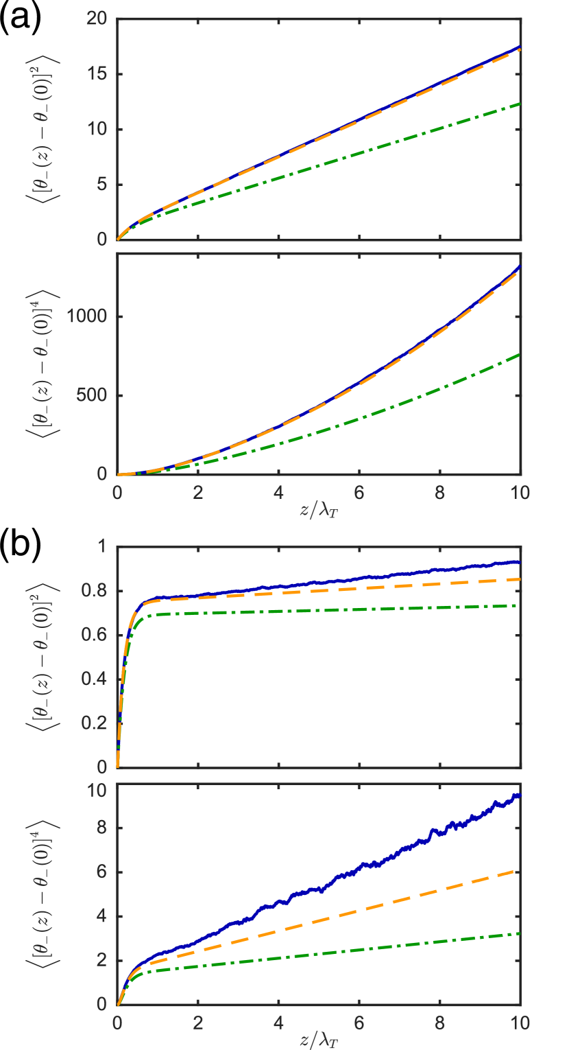
For small and intermediate phase-locking the results for the full model agree with the predictions of the SG model with the rescaled parameters and Beck et al. (2018). Here represents the regularized mean inverse density (in dimensionless units), for symmetry reasons the expectation value is the same for . Without regularization, diverges logarithmically. Different ways to regularize have been tested and all yielded very close results. Fig. 1(a) shows the results for , which corresponds to intermediate phase locking. One sees good agreement between the results for the full calculation and the rescaled SG model. For stronger phase-locking deviations are clearly visible [Fig. 1(b)].
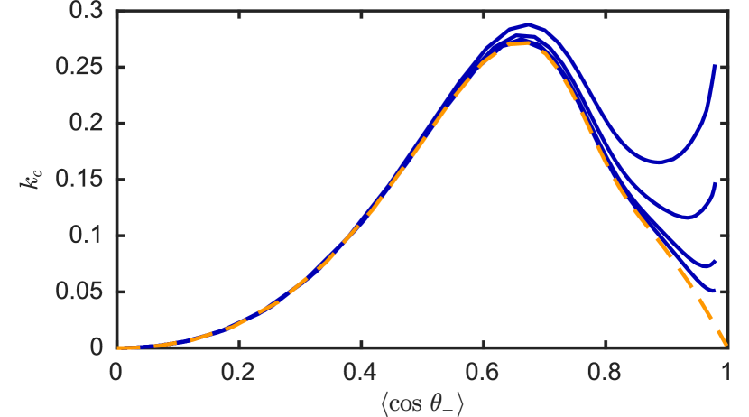
Note that it is not possible to achieve agreement by using a different rescaling of parameters in the strong-coupling case. One can best see this from single-point expectation values calculated from (6) . They only depend on for the SG model and on and for the coupled quasicondensates. We analyze the circular kurtosis Fisher (1993)
| (16) |
which is a measure for the non-Gaussianity of the underlying distribution of . Fig. 2 shows as a function of . One can see the deviation of the exact results from the predictions of the SG model for .
The deviation from the SG theory is bigger for smaller values of , i.e. for higher temperatures or lower densities. The density fluctuations are the physical reason. The higher (i.e., the more pronounced the effect of interatomic repulsion), the more suppressed are the density fluctuations. The accuracy of the SG description is thus increased. The good agreement of the experimental data of Ref. Schweigler et al. (2017) with the SG model can be explained by rather a high value . For the discrepancy between the full description of two coupled quasicondensates and the SG model becomes well pronounced. However, experimental measurements in this parameter regime are challenging due to the finite resolution of the imaging system.
Note that the non-Gaussianity for intermediate phase-locking (intermediate values of ) and strong phase-locking () has different physical origins. For intermediate phase-locking, as a function of for fixed is non-Gaussian in the relevant range of and (close to 1). For strong phase-locking this is not the case any more. The distribution of for different points , is approximately Gaussian, with the variance depending on , . Therefore, averaging over different points leads to an overall distribution for which is non-Gaussian.
To conclude, we have developed a versatile method for calculating thermal expectation values for 1D systems. We applied the method to the case of two tunnel-coupled 1D quasicondensates. We identified the cases when this system can be described by the simpler sine-Gordon model and when this description breaks down.
Our non-perturbative method is applicable to basically all stable continuous 1D bosonic systems with local interactions as long as thermal fluctuations describable by classical fields dominate. Additional requirements are that the system is homogeneous and non-relativistic. The main advantage of the presented method is its computational efficiency. Calculating the realizations used for Fig. 1 takes around 2 hours on a desktop computer, which is at least by an order of magnitude shorter than what more traditional methods like stochastic Gross-Pitaevskii (SGPE) Blakie et al. (2008) would need. Moreover, we should mention the robustness of our method in the presence of (quasi)topological excitation. Such excitations often comprise a problem when using methods based on the evolution in presence of a noise term (SGPE) or some sort of Metropolis-Hastings algorithm Grišins and Mazets (2014). We therefore believe that our method will find its application in a broad research area.
The authors thank S. Erne, V. Kasper, and J. Schmiedmayer for helpful discussions. We acknowledge financial support by the by the Wiener Wissenschafts und Technologie Fonds (WWTF) via the grant MA16-066 and by the EU via the ERC advanced grant QuantumRelax (GA 320975). This work was also supported by the Austrian Science Fund (FWF) via the project P 25329-N27 (S.B., I.M.), the SFB ISOQUANT No. I 3010-N27, and the Doctoral Programmes W 1245-N25 “Dissipation und Dispersion in nichtlinearen partiellen Differentialgleichungen” (S.B.) and W 1210-N25 CoQuS (T.S.).
References
- Giamarchi (2004) T. Giamarchi, Quantum physics in one dimension (Clarendon Press, Oxford, 2004).
- Cazalilla et al. (2011) M. A. Cazalilla, R. Citro, T. Giamarchi, E. Orignac, and M. Rigol, Rev. Mod. Phys. 83, 1405 (2011).
- Bloch et al. (2008) I. Bloch, J. Dalibard, and W. Zwerger, Rev. Mod. Phys. 80, 885 (2008).
- Proukakis et al. (2017) N. P. Proukakis, D. W. Snoke, and P. B. Littlewood, Universal Themes of Bose-Einstein Condensation (Cambridge University Press, Cambridge, 2017).
- Chang et al. (2008) D. Chang, V. Gritsev, G. Morigi, V. Vuletić, M. Lukin, and E. Demler, Nat. Phys. 4, 884 (2008).
- Wada et al. (2001) N. Wada, J. Taniguchi, H. Ikegami, S. Inagaki, and Y. Fukushima, Phys. Rev. Lett. 86, 4322 (2001).
- Lieb and Liniger (1963) E. H. Lieb and W. Liniger, Phys. Rev. 130, 1605 (1963).
- Lieb (1963) E. Lieb, Phys. Rev. 130, 1616 (1963).
- Luttinger (1963) J. M. Luttinger, J. Math. Phys. 4, 1154 (1963).
- Langen et al. (2015) T. Langen, S. Erne, R. Geiger, B. Rauer, T. Schweigler, M. Kuhnert, W. Rohringer, I. E. Mazets, T. Gasenzer, and J. Schmiedmayer, Science 348, 207 (2015).
- Bordia et al. (2017) P. Bordia, H. Lüschen, U. Schneider, M. Knap, and I. Bloch, Nat. Phys. 13, 460 (2017).
- Rauer et al. (2018) B. Rauer, S. Erne, T. Schweigler, F. Cataldini, M. Tajik, and J. Schmiedmayer, Science 360, 307 (2018).
- Schweigler et al. (2017) T. Schweigler, V. Kasper, S. Erne, I. Mazets, B. Rauer, F. Cataldini, T. Langen, T. Gasenzer, J. Berges, and J. Schmiedmayer, Nature 545, 323 (2017).
- Stimming et al. (2010) H.-P. Stimming, N. J. Mauser, J. Schmiedmayer, and I. E. Mazets, Phys. Rev. Lett. 105, 015301 (2010).
- Goldstein and Meystre (1997) E. V. Goldstein and P. Meystre, Phys. Rev. A 55, 2935 (1997).
- Whitlock and Bouchoule (2003) N. K. Whitlock and I. Bouchoule, Phys. Rev. A 68, 053609 (2003).
- Beck et al. (2018) S. Beck, I. E. Mazets, and T. Schweigler, Phys. Rev. A 98, 023613 (2018).
- Scalapino et al. (1972) D. J. Scalapino, M. Sears, and R. A. Ferrell, Phys. Rev. B 6, 3409 (1972).
- Krumhansl and Schrieffer (1975) J. A. Krumhansl and J. R. Schrieffer, Phys. Rev. B 11, 3535 (1975).
- Currie et al. (1980) J. F. Currie, J. A. Krumhansl, A. R. Bishop, and S. E. Trullinger, Phys. Rev. B 22, 477 (1980).
- Risken (1989) H. Risken, The Fokker-Planck Equation, 2nd ed., Springer Series in Synergetics (Springer, Berlin, 1989).
- Gardiner (1985) C. Gardiner, Handbook of stochastic methods (Springer, Berlin, 1985).
- Mora and Castin (2003) C. Mora and Y. Castin, Phys. Rev. A 67, 053615 (2003).
- Grišins and Mazets (2013) P. Grišins and I. E. Mazets, Phys. Rev. A 87, 013629 (2013).
- Schumm et al. (2005) T. Schumm, S. Hofferberth, L. M. Andersson, S. Wildermuth, S. Groth, I. Bar-Joseph, J. Schmiedmayer, and P. Kruger, Nat. Phys. 1, 57 (2005).
- Gritsev et al. (2007) V. Gritsev, A. Polkovnikov, and E. Demler, Phys. Rev. B 75, 174511 (2007).
- Fisher (1993) N. I. Fisher, Statistical Analysis of Circular Data (Cambridge University Press, Cambridge, 1993).
- Blakie et al. (2008) P. Blakie, A. Bradley, M. Davis, R. Ballagh, and C. Gardiner, Adv. Phys. 57, 363 (2008).
- Grišins and Mazets (2014) P. Grišins and I. Mazets, Comput. Phys. Commun. 185, 1926 (2014).