Does the gravitomagnetic monopole exist? A clue from a black hole x-ray binary

Abstract

The gravitomagnetic monopole is the proposed gravitational analogue of Dirac’s magnetic monopole. However, an observational evidence of this aspect of fundamental physics was elusive. Here, we employ a technique involving three primary X-ray observational methods used to measure a black hole spin to search for the gravitomagnetic monopole. These independent methods give significantly different spin values for an accreting black hole. We demonstrate that the inclusion of one extra parameter due to the gravitomagnetic monopole not only makes the spin and other parameter values inferred from the three methods consistent with each other but also makes the inferred black hole mass consistent with an independently measured value. We argue that this first indication of the gravitomagnetic monopole, within our paradigm, is not a result of fine tuning.

I Introduction

The gravitational analogue of Dirac’s magnetic monopole dirac ; saha is known as the gravitomagnetic monopole zee , which, if detected, can open a new area of research in physics. Historically, Newmann et al. discovered a stationary and spherically symmetric exact solution (now known as the NUT solution) of Einstein equation, that contains the gravitomagnetic monopole or the so-called NUT (Newman, Unti and Tamburino nut ) parameter ahm ; bini . Note that Einstein-Hilbert action requires no modification rs2 to accommodate the gravitomagnetic monopole. Demianski and Newman found that the NUT spacetime is produced by a ‘dual mass’ dn or the gravitomagnetic charge/monopole. Bonnor bon physically interpreted it as ‘a linear source of pure angular momentum’ dow ; rs , i.e., ‘a massless rotating rod’. Moreover, the NUT spacetime is free of curvature singularities rs2 , and the mass (or the so-called gravitoelectric charge) quantization zee is possible due to the presence of the gravitomagnetic charge, which is a general feature mp of a spacetime with dual mass rs2 ; rs . Therefore, gravitomagnetic monopole or NUT parameter is a fundamental aspect of physics.

While the existence of gravitomagnetic monopole is an exciting possibility, to the best of our knowledge, a serious effort to search for it among the astronomical objects has not been made so far. Lynden-Bell and Nouri-Zonoz lnbl , who were possibly the first to motivate such an investigation, argued that the best place to look for the gravitomagnetic monopole is in the spectra of supernovae, quasars, or active galactic nuclei (see also kag ). But practical ways to detect the gravitomagnetic monopole in nature, if it exists, were not proposed. In this paper, we demonstrate that X-ray observations of a black hole X-ray binary (BHXB), i.e., an accreting stellar-mass collapsed object, can provide a way to detect a non-zero NUT parameter or the gravitomagnetic monopole. This is because, while the spacetime of such a spinning collapsed object (a black hole, or even a naked singularity) is usually described with the Kerr metric kerr , the Kerr geometry may naturally contain the NUT parameter along with the mass and the angular momentum, and be known as the Kerr-Taub-NUT (KTN) spacetime ml , which is geometrically a stationary, axisymmetric vacuum solution of Einstein equation, and reduces to the Kerr spacetime if the NUT parameter is zero. Therefore, identification of a collapsed object having the KTN spacetime with a non-zero NUT parameter can be ideal to establish the existence of the gravitomagnetic monopole. In this paper, we demonstrate that X-ray observations of a black hole X-ray binary (BHXB), i.e., an accreting stellar-mass collapsed object, can provide a way to infer and measure the NUT parameter. Note that, while the collapsed object is usually thought to be a black hole, i.e., a singularity covered by an event horizon, here we do not exclude the possibility that it could also be a naked or uncovered singularity in some cases ckp .

We search for the gravitomagnetic monopole using three independent X-ray observational methods used to measure a black hole spin. We briefly discuss these methods in Sec.II. In our study, we use fundamental frequencies, ISCO radius and gravitational redshift. We derive and provide formulae for some of these quantities for various spacetimes in Sec.III. In Sec.IV, we use these expressions to explore the possibility of the non-zero NUT parameter in a BHXB : GRO J1655–40. The additional plausible solutions of our work are discussed in Sec.V and finally, we conclude in Sec.VI.

II Materials and Methods

Measurement of the NUT parameter can be done by combining several methods, which are used to measure the spin parameter (or Kerr parameter) $a/M$ of an accreting collapsed object. Here, $a/M=J/M^{2}$, where $M$ and $J$ are the collapsed object mass and angular momentum respectively. Note that measuring $a/M$ can be very useful to probe the strong gravity regime and to characterize the collapsed object, and a significant effort in astronomy has been made for such measurements RemillardMcClintock2006 ; Miller2007 ; bs14 . However, different methods to measure $a/M$ do not sometimes give consistent results, which make these methods unreliable. In this paper, we demonstrate that these results can be consistent with each other, if we allow a non-zero NUT parameter value.

Some of the X-ray spectral and timing features, originating from the accreted matter within a few gravitational radii of a collapsed object in a BHXB, can be used to measure the spin parameter $a/M$ RemillardMcClintock2006 ; Miller2007 ; bs14 . There are two main spectral methods for $a/M$ estimation: (1) using broad relativistic iron K$\alpha$ spectral emission line Miller2007 , and (2) using continuum X-ray spectrum RemillardMcClintock2006 . There is also a timing method based on the relativistic precession model (RPM) of quasi-periodic oscillations (QPOs) of X-ray intensity motta40 . We briefly discuss these methods below.

A broad relativistic iron K$\alpha$ spectral emission line in X-rays is observed from many BHXBs, and such a fluorescent line is believed to originate from the reflection of hard X-rays from the inner part of the geometrically thin accretion disk. This intrinsically narrow iron line ($6.4-6.97$ keV) is broadened, becomes asymmetric and shifted towards lower energies by physical effects, such as Doppler effect, special relativistic beaming and gravitational redshift ReynoldsNowak2003 ; Miller2007 . Note that it is primarily the extent of the red wing of the line that determines the observed constraint on $a/M$ Reisetal2009 . This is because this red wing extent gives a measure of the gravitational redshift at the disk inner edge radius $r_{\rm in}$ (as this redshift in the disk is the maximum at the inner edge), and for $r_{\rm in}=r_{\rm ISCO}$ ($r_{\rm ISCO}$ is the innermost stable circular orbit (ISCO) radius), the $a/M$ value can be inferred for a prograde accretion disk in the Kerr spacetime (Eqs. 11 and 12).

The modeling of the observed continuum X-ray spectrum can also be used to constrain $a/M$. In this method, the thermal spectral component from the accretion disk is fit with a relativistic thin-disk model, and this gives a measure of the $r_{\rm in}$, if the source distance ($D$) and the accretion disk inclination angle ($i$) are independently measured FragosMcClintock2015 . Then from a known $M$ value, $r_{\rm ISCO}/M$, and hence $a/M$, can be inferred assuming Kerr spacetime.

The QPO-based timing method uses three observed features to estimate $a/M$: (a) the upper high-frequency (HF) QPO, (b) the lower HFQPO, and (c) the type-C low-frequency (LF) QPO motta40 . HFQPOs are rare, and they are observed in the frequency range of $\sim 40-450$ Hz Bellonietal2012 . Type-C QPO is the most common LFQPO, and it is observed in the frequency range of $\sim 0.01-30$ Hz bs14 . According to this method based on the relativistic precession model (RPM), which was first proposed for accreting neutron stars by StellaVietri1998 ; StellaVietri1999 , the Type-C QPO frequency is identified with the LT precession frequency ($\nu_{\rm LT}$), and the upper and lower HFQPO frequencies are identified with the orbital frequency ($\nu_{\phi}$) and the periastron precession frequency ($\nu_{\rm per}$) respectively motta40 . For the Kerr spacetime, each of these three frequencies is a function of three parameters: $M$, $a/M$ and the radial coordinate $r_{\rm qpo}$ of the location of origin of these QPOs. Hence, the RPM method can provide not only the $a/M$ value, but also the values of $M$ and $r_{\rm qpo}$ motta40 .

So far the RPM method could be fully applied for one BHXB (GRO J1655–40), because, to the best of our knowledge, the three above-mentioned QPOs could be simultaneously observed only from this BHXB motta40 . The mass of the collapsed object of GRO J1655–40 is either $(6.3\pm 0.5)M_{\odot}$ Greeneetal2001 or $(5.4\pm 0.3)M_{\odot}$ beer (it is not yet clear which one is more reliable; FragosMcClintock2015 ). According to the RPM, the observed frequencies of the above mentioned three simultaneous QPOs imply $\nu_{\phi}=440$ Hz, $\nu_{\rm per}=300$ Hz and $\nu_{\rm LT}=17$ Hz for GRO J1655–40. Using these frequencies, motta40 determined $a/M\approx 0.286\pm 0.003$, $M\approx(5.31\pm 0.07)M_{\odot}$ and $r_{\rm qpo}\approx(5.68\pm 0.04)~{}M$. Moreover, the inferred $M\approx 5.31M_{\odot}$ is consistent with an independently measured mass $(5.4\pm 0.3)M_{\odot}$ beer , which indicates the reliability of the RPM method and the corresponding inferred parameter values for GRO J1655–40.

While such a QPO-based estimation of the $a/M$ value is model dependent, we would like to note that a recent observation of a variation of the relativistic iron line energy with the phase of the Type-C QPO from the BHXB H1743-322 supports that this QPO is caused by the LT precession (in16 ; see also MillerHoman2005 ; Schnittmanetal2006 ), as considered in the RPM. Note that this may require a tilted inner disk, which has recently been theoretically shown to be possible ChakrabortyBhattacharyya2017 . Besides, while the RPM interpretation of HFQPOs is not unique, the reliability of the RPM method can be tested by comparing the mass inferred from this method with an independently measured $M$ value (as mentioned in the previous paragraph). Moreover, motta40 listed some HFQPOs simultaneously observed with Type-C QPOs from GRO J1655–40. They identified some of these HFQPOs as lower HFQPOs, and some as upper HFQPOs. For the $M$ and $a/M$ values inferred by motta40 , and assuming the Type-C QPO frequencies to be $\nu_{\rm LT}$, a radius of origin for each of these LFQPOs can be calculated for Kerr spacetime (see Sec. III). In their Fig. 5, motta40 showed that, the simultaneous lower HFQPO frequencies match well with the $\nu_{\rm per}$ values at the corresponding radii for the same $M$ and $a/M$ values. Similarly, the simultaneous upper HFQPO frequencies match well with the $\nu_{\phi}$ values at the corresponding radii. These provide a support for the RPM for QPOs.

GRO J1655–40 is currently the only BHXB, for which all the three above mentioned $a/M$ estimation methods are available, and hence, this source provides a unique opportunity to test the reliability of these methods by comparing the three estimated $a/M$ values. The timing method gives $a/M\approx 0.286\pm 0.003$ motta40 , the line spectrum method gives $a/M\approx 0.90-0.99$ Reisetal2009 , and the continuum spectrum method gives $a/M\approx 0.65-0.75$ (using $M\approx 6.3M_{\odot}$, $D\approx 3.2$ kpc, $i\approx 70^{\circ}.2$; sha ) for GRO J1655–40. Therefore, not only the $a/M$ value inferred from the timing method is inconsistent with those inferred from the spectral methods, but also the results from the two spectral methods are grossly inconsistent with each other. Even if $M\approx 5.4M_{\odot}$ beer were used, which would be consistent with the finding from the RPM method motta40 , the continuum spectrum method would give an $a/M$ range of $0.50-0.63$. This is inconsistent with the results from both the RPM method and the line spectrum method. These suggest that all three methods could be unreliable. If true, this will make some of our current understandings of black holes doubtful, will deprive us of reliable $a/M$ measurement methods, and could impact the future plans of X-ray observations of BHXBs.

Can it be possible that these methods are actually reliable (as indicated by the works reported in a large volume of publications; e.g., ReynoldsNowak2003 ; Miller2007 ; RemillardMcClintock2006 ), but they are missing an essential ingredient? Here we explore an exciting possibility that the inclusion of gravitomagnetic monopole may make the results from three methods consistent, thus suggesting that such a monopole exists in nature. For this purpose, we allow non-zero NUT parameter values (implying gravitomagnetic monopole) in our calculations, by considering the KTN spacetime, instead of the previously used Kerr spacetime. Note that the former spacetime, having one additional parameter, i.e., the NUT parameter $n/M$, is a generalized version of the latter. Before testing this new idea, let us first consider the KTN metric and derive the corresponding three fundamental frequencies: orbital frequency $\nu_{\phi}$, radial epicyclic frequency $\nu_{r}$ and vertical epicyclic frequency $\nu_{\theta}$.

III Fundamental frequencies in Kerr-Taub-NUT spacetime

The metric of the KTN spacetime is expressed as ml

$$ds^{2}=-\frac{\Delta}{p^{2}}(dt-Ad\phi)^{2}+\frac{p^{2}}{\Delta}dr^{2}+p^{2}d\theta^{2}+\frac{1}{p^{2}}\sin^{2}\theta(adt-Bd\phi)^{2}$$ (1)

with

$$\Delta = r^{2}-2Mr+a^{2}-n^{2},\,\,\,\,\,\,\,\,\,p^{2}=r^{2}+(n+a\cos\theta)^{2},$$

$$A = a\sin^{2}\theta-2n\cos\theta,\,\,\,\,\,\,\,\,B=r^{2}+a^{2}+n^{2},$$ (2)

where $M$ is the mass, $a/M$ is the Kerr parameter and $n/M$ is the NUT parameter.

Now, substituting the metric components ($g_{\mu\nu}$) of KTN spacetime in Eqs. (22-24) of Appendix A, we can obtain the three fundamental frequencies. The orbital frequency can be written as cc2

$$\Omega_{\phi}^{\rm KTN}=2\pi\nu_{\phi}^{\rm KTN}=\pm\frac{m^{\frac{1}{2}}}{r^{\frac{1}{2}}~{}(r^{2}+n^{2})\pm a~{}m^{\frac{1}{2}}},$$ (3)

where $m=M~{}(r^{2}-n^{2})+2~{}n^{2}r$. In all the equations here, the upper sign is applicable for the prograde orbits (which we use throughout in our paper) and the lower sign is applicable for the retrograde orbits.

Similarly, radial and vertical epicyclic frequencies are (which, to the best of our knowledge, reported for the first time here):

$$\nu_{r}^{\rm KTN} = \frac{\nu_{\phi}^{\rm KTN}}{m^{\frac{1}{2}}~{}(r^{2}+n^{2})}.\left[M(r^{6}-n^{6}+15n^{4}r^{2}-15n^{2}r^{4})-2M^{2}r(3r^{4}-2n^{2}r^{2}+3n^{4})-16n^{4}r^{3}\right.$$ (4)

$$\left.\pm 8ar^{\frac{3}{2}}m^{\frac{3}{2}}+a^{2}\left\{M(n^{4}+6n^{2}r^{2}-3r^{4})-8n^{2}r^{3}\right\}\right]^{\frac{1}{2}}$$

and

$$\nu_{\theta}^{\rm KTN} = \frac{\nu_{\phi}^{\rm KTN}}{m^{\frac{1}{2}}~{}(r^{2}+n^{2})}.\left[M(r^{6}-n^{6}+15n^{4}r^{2}-15n^{2}r^{4})+2n^{2}r(3r^{4}-2n^{2}r^{2}+3n^{4})+16M^{2}n^{2}r^{3}\right.$$ (5)

$$\left.\mp 4ar^{\frac{1}{2}}m^{\frac{1}{2}}(n^{2}+Mr)(n^{2}+r^{2})-a^{2}\left\{M(n^{4}+6n^{2}r^{2}-3r^{4})-8n^{2}r^{3}\right\}\right]^{\frac{1}{2}}$$

respectively.

Setting the square of Eq. (4) equal to zero (i.e., $[\nu_{r}^{\rm KTN}]^{2}=0$), we obtain the innermost stable circular orbit (ISCO) condition as follows cc2 :

$$M(r^{6}-n^{6}+15n^{4}r^{2}-15n^{2}r^{4})-2M^{2}r(3r^{4}-2n^{2}r^{2}+3n^{4})-16n^{4}r^{3}$$

$$\pm 8ar^{\frac{3}{2}}m^{\frac{3}{2}}+a^{2}\left\{M(n^{4}+6n^{2}r^{2}-3r^{4})-8n^{2}r^{3}\right\}=0.$$

Gravitational redshift in KTN spacetime

The gravitational redshift in the KTN spacetime is expressed as (using Eq. 26 of Appendix A):

$$Z^{\rm KTN}=\frac{r^{\frac{1}{2}}(r^{2}+n^{2})+a~{}m^{\frac{1}{2}}}{\left[(r^{2}+n^{2})~{}\left\{r(r^{2}-3n^{2})+M(n^{2}-3r^{2})+2a(mr)^{\frac{1}{2}}\right\}\right]^{\frac{1}{2}}}.$$ (7)

SPECIAL CASES

III.1 Kerr spacetime ($n=0$ and $a\neq 0$)

Now, in the Kerr spacetime ($n=0$), Eqs. (3-5) reduce to ok ; ka

$$\Omega_{\phi}^{\rm Kerr}=2\pi\nu_{\phi}^{\rm Kerr}=\pm\frac{M^{\frac{1}{2}}}{r^{\frac{3}{2}}\pm a~{}M^{\frac{1}{2}}},$$ (8)

$$\nu_{r}^{\rm Kerr}=\frac{\nu_{\phi}^{\rm Kerr}}{r}.\left[r^{2}-6Mr\pm 8ar^{\frac{1}{2}}M^{\frac{1}{2}}-3a^{2}\right]^{\frac{1}{2}}$$ (9)

and

$$\nu_{\theta}^{\rm Kerr}=\frac{\nu_{\phi}^{\rm Kerr}}{r}.\left[r^{2}\mp 4ar^{\frac{1}{2}}M^{\frac{1}{2}}+3a^{2}\right]^{\frac{1}{2}}$$ (10)

respectively.

Setting the square of Eq. (9) equal to zero, we obtain the ISCO condition ch :

$$r^{2}-6Mr\pm 8ar^{\frac{1}{2}}M^{\frac{1}{2}}-3a^{2}=0.$$ (11)

Gravitational redshift in Kerr spacetime

In Kerr spacetime, gravitational redshift equation (Eq. 7) reduces to

$$Z^{\rm Kerr}=\frac{r^{\frac{3}{2}}+a~{}M^{\frac{1}{2}}}{r^{\frac{1}{2}}\left[r^{2}-3Mr+2a(Mr)^{\frac{1}{2}}\right]^{\frac{1}{2}}}.$$ (12)

From the above expression, we can obtain the well-known redshift expression in the Schwarzschild spacetime: $Z^{\rm Schwarzschild}=\left(1-\frac{3M}{r}\right)^{-\frac{1}{2}}$.

III.2 NUT spacetime ($a=0$ and $n\neq 0$)

In the case of NUT spacetime ($a=0$), Eqs. (3-5) reduce to cc2

$$\Omega_{\phi}^{\rm NUT}=2\pi\nu_{\phi}^{\rm NUT}=\pm\frac{m^{\frac{1}{2}}}{r^{\frac{1}{2}}~{}(r^{2}+n^{2})},$$ (13)

$$\nu_{r}^{\rm NUT}=\frac{\nu_{\phi}^{\rm NUT}}{m^{\frac{1}{2}}~{}(r^{2}+n^{2})}.\left[M(r^{6}-n^{6}+15n^{4}r^{2}-15n^{2}r^{4})-2M^{2}r(3r^{4}-2n^{2}r^{2}+3n^{4})-16n^{4}r^{3}\right]^{\frac{1}{2}}$$

(14)

and

$$\nu_{\theta}^{\rm NUT} = \frac{\nu_{\phi}^{\rm NUT}}{m^{\frac{1}{2}}~{}(r^{2}+n^{2})}.\left[M(r^{6}-n^{6}+15n^{4}r^{2}-15n^{2}r^{4})+2n^{2}r(3r^{4}-2n^{2}r^{2}+3n^{4})+16M^{2}n^{2}r^{3}\right]^{\frac{1}{2}}$$

respectively. Here $m=M~{}(r^{2}-n^{2})+2~{}n^{2}r$.

Setting the square of Eq. (14) equal to zero, one can obtain the ISCO condition:

$$M(r^{6}-n^{6}+15n^{4}r^{2}-15n^{2}r^{4})-2M^{2}r(3r^{4}-2n^{2}r^{2}+3n^{4})-16n^{4}r^{3}=0.$$ (16)

Remarkably, in general $\nu_{\phi}^{\rm NUT}\neq\nu_{\theta}^{\rm NUT}$ in the NUT spacetime. This means that the LT precession frequency $\nu_{\rm LT}^{\rm NUT}~{}(\equiv\nu_{\phi}^{\rm NUT}-\nu_{\theta}^{\rm NUT}$) does not vanish in NUT spacetime, i.e., inertial frames are dragged due to the presence of a non-zero NUT charge, although the spacetime is non-rotating ($a=0$).

Gravitational redshift in NUT spacetime

In NUT spacetime, the gravitational redshift equation (Eq. 7) reduces to

$$Z^{\rm NUT}=\left[\frac{r(r^{2}+n^{2})}{r(r^{2}-3n^{2})+M(n^{2}-3r^{2})}\right]^{\frac{1}{2}}.$$ (17)

IV Exploring the possibility of non-zero NUT parameter in GRO J1655-40

The three fundamental frequencies (Eqs. 8-10) for the Kerr spacetime and for infinitesimally eccentric and tilted orbits were used by motta40 for $a/M$ estimation using the RPM method. Since we use the KTN spacetime instead of the Kerr spacetime, here we use the expressions of these frequencies (see Eqs. 3–5) corresponding to the KTN spacetime. One can now derive the periastron precession frequency $\nu_{\rm per}^{\rm KTN}(=\nu_{\phi}^{\rm KTN}-\nu_{r}^{\rm KTN}$) and the Lense-Thirring (LT) precession frequency $\nu_{\rm LT}^{\rm KTN}(=\nu_{\phi}^{\rm KTN}-\nu_{\theta}^{\rm KTN}$) using these three fundamental frequencies. Besides, the condition to derive the radius of the innermost stable circular orbit $r_{\rm ISCO}$ and the expression of the gravitational redshift for the KTN spacetime are given by Eq. (LABEL:isco) (see also cc2 ) and Eq. (7) respectively.

Now, we apply the RPM method to GRO J1655–40 using the KTN frequencies. Following motta40 , we consider

$$\nu_{\phi}^{\rm KTN}=440~{}{\rm Hz};\,\,\nu_{\rm per}^{\rm KTN}=300~{}{\rm Hz};\,\,\,\,\nu_{\rm LT}^{\rm KTN}=17~{}{\rm Hz}$$ (18)

for GRO J1655–40, and using the expressions given in Eqs. (3–5), we can solve Eqs.(18) for $a/M$, $M$ and the radius $r_{\rm qpo}$ of QPO origin for a given $n/M$ value. For $n/M=0$, we naturally recover the $a/M$, $M$ and $r_{\rm qpo}$ values reported in motta40 . Now, if we increase $n/M$ from zero, $a/M$ also increases (while Eq. 18 is satisfied), and hence the RPM method gives an allowed $n/M$ versus $a/M$ relation (shown by the green dotted curve in Fig. 1) for GRO J1655–40.

Note that the range of $a/M$ is $0-1$ for a Kerr black hole. For $a/M>1$, the radii of the horizons $r_{\pm}(=M\pm\sqrt{M^{2}-a^{2}}$) become imaginary, and hence the collapsed object becomes a naked singularity ckj ; ckp . However, for a KTN collapsed object the radii of the horizons are $M\pm\sqrt{M^{2}+n^{2}-a^{2}}$, and hence the condition for a naked singularity is $a/M>\sqrt{1+(n/M)^{2}}$ wei . This condition is shown by a black dashed line in Fig. 1, which divides the $n/M$ versus $a/M$ space into a black hole region and a naked singularity region for the KTN spacetime. This figure shows that $a/M$ can easily be much higher than $1$ for a black hole for non-zero $n/M$ values. We find that the $n/M$ versus $a/M$ curve allowed from the RPM method for GRO J1655–40 extends into the naked singularity region (Fig. 1). Note that black holes and naked singularities could coexist in nature JoshiMalafarina2011 , and hence the detection of an event horizon of a collapsed object does not rule out the possibility of the existence of a naked singularity, and vice versa.

Figure 1: The NUT parameter ($n/M$) versus the spin parameter ($a/M$) space, which is divided into a black hole region and a naked singularity region (see text) by the black dashed line. The $n/M$ versus $a/M$ constraints for GRO J1655–40 are given by (1) the green dotted curve (using only the RPM timing method), (2) the red dotted curve (using the RPM timing and line spectrum methods), and (3) the blue solid curve (using the RPM timing and continuum spectrum methods). A zoomed version of the latter two is shown in the inset for clarity. This figure shows that there is a range of $n/M$ and $a/M$ values for GRO J1655–40 allowed by all the three methods.

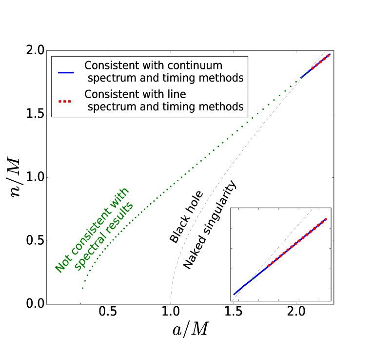
Let us now explore if non-zero $n/M$ values can make the $a/M$ ranges inferred from the RPM method and the line spectrum method consistent with each other for GRO J1655–40, and if so, what constraints of $a/M$ and $n/M$ can be obtained. We do this by combining these two methods as described below. The $a/M$ range for GRO J1655–40 was estimated to be $\approx 0.90-0.99$ using the line spectrum method Reisetal2009 . But this estimation assumed Kerr spacetime, while we need to constrain parameters in the KTN spacetime, to allow non-zero $n/M$ values. Therefore, using Eqs. (11) and (12), we calculate the gravitational redshift range ($\approx 2.70-6.08$) from the reported $a/M$ range ($\approx 0.90-0.99$). This gravitational redshift could be directly inferred from the extent of the red wing of the observed broad iron line (see Sec. II), and itself does not depend on Kerr spacetime. Therefore, we treat this gravitational redshift range ($\approx 2.70-6.08$) as the primary observational constraint, independent of the Kerr spacetime. Using this primary constraint and assuming the KTN spacetime, i.e., $Z^{\rm KTN}{\rm(at}~{}r_{\rm ISCO})=2.70-6.08$ (L.H.S. is given by Eqs. LABEL:isco and 7), and using Eq. (18), we solve for $M$, $a/M$, $n/M$, $r_{\rm ISCO}/M$ and $r_{\rm qpo}$ (in unit of $M$). This solution gives the following constraints for GRO J1655–40, which are consistent with both the RPM method and the line spectrum method: $M\approx 6.76-6.83M_{\odot}$, $a/M\approx 2.12-2.27$, $n/M\approx 1.86-1.97$ and $r_{\rm qpo}/M\approx 4.99-5.04$. While the non-zero $n/M$ range implies the existence of the gravitomagnetic monopole, the red dotted curve in Fig. 1 shows that this $n/M$ versus $a/M$ range implies a naked singularity. The $M$ range is consistent with an independently measured mass ($[6.3\pm 0.5]M_{\odot}$; Greeneetal2001 ) for GRO J1655–40, which provides a confirmation of the reliability of our method and results.

Next, we explore if the $a/M$ ranges inferred from the RPM method and the continuum spectrum method can be consistent with each other for GRO J1655–40, if non-zero $n/M$ values are allowed. For GRO J1655–40, the $a/M$ range estimated from the continuum spectrum method is $\approx 0.65-0.75$ sha , assuming the Kerr spacetime. Therefore, as argued in the previous paragraph, we need a primary observational constraint, independent of the Kerr spacetime, so that the more general KTN spacetime for non-zero $n/M$ values can be used. For GRO J1655–40, we find that the quoted $a/M$ range of $\approx 0.65-0.75$ sha was inferred from an $r_{\rm ISCO}$ range of $\approx 29.8-34.2$ km and using $M=6.3M_{\odot}$. As mentioned in Sec. II, $r_{\rm ISCO}$ could directly (i.e., independent of the Kerr spacetime) be inferred from the observed spectrum using the known source distance ($D$) and the accretion disk inclination angle ($i$) values. Therefore, using $r_{\rm ISCO}=29.8-34.2$ km as the primary constraint and assuming the KTN spacetime (e.g., using Eq. LABEL:isco), and using Eq. (18), we solve for $M$, $a/M$, $n/M$, $r_{\rm ISCO}/M$ and $r_{\rm qpo}/M$. Consequently, the following parameter constraints could be obtained: $M\approx 6.79-6.86M_{\odot}$, $a/M\approx 2.04-2.21$, $n/M\approx 1.79-1.93$ and $r_{\rm qpo}/M\approx 4.96-5.02$. These parameter ranges are largely overlapping with those obtained from the combined RPM and line spectrum method. We find that even for this combined RPM and continuum spectrum method, the non-zero $n/M$ range implies the gravitomagnetic monopole, the mass is consistent with an independently measured mass ($[6.3\pm 0.5]M_{\odot}$; Greeneetal2001 ) for GRO J1655–40, and the $n/M$ versus $a/M$ curve (the blue solid curve in Fig. 1) mainly implies a naked singularity, although a black hole is also possible.

V Other probable solutions with non-zero NUT parameter in GRO J1655–40

It should be noted that there is a possibility to obtain other solutions with the non-zero NUT parameter, and consequently, other sets of parameter constraints. This is because the LT precession frequency can change sign as one moves outwards from the collapsed object. This implies the same absolute value of the LT precession frequency at three radius values. In this section, we discuss on these other plausible solutions, and show that those solutions are not viable.

The three simultaneous QPOs from GRO J1655–40 were used by Motta et al. motta40 to infer the parameter values of this source using the RPM method. These parameter values were used in Fig. 5 of their paper to make the theoretical frequency versus radius curves (three curves for three frequencies). Then they collected pairs of two simultaneously observed QPOs (one is LFQPO and another one is HFQPO) from this source. Among the HFQPOs, they considered two as upper HFQPOs, and rest as lower HFQPOs. Using an LFQPO frequency, and the theoretical LT precession frequency curve (drawn using the inferred parameter values from three simultaneous QPOs, as mentioned above), the radius of origin of the LFQPO is calculated. Then if it is assumed that the simultaneously observed HFQPO is originated from the same radius, the frequency of the HFQPO comes out to be more-or-less consistent with the theoretical frequency curve, as required by RPM (see Fig. 5 of Motta et al. motta40 ). This provides a support for the RPM method to estimate $a/M$.

Figure 2: LT precession frequency (dotted line), periastron precession frequency (dashed line) and orbital frequency (dot-dashed line) as a function of the distance $(r)$ around a KTN collapsed object as predicted by the RPM. The lines are drawn for $M=6.83~{}M_{\odot}$, $a=2.12~{}M$ and $n=1.86~{}M$. The observed QPO frequencies (red, black and green points in the plot) are from the Table 1 of Motta et al. motta40 . This plot may be compared with Fig. 5 of Motta et al. motta40 (see Sec. V).

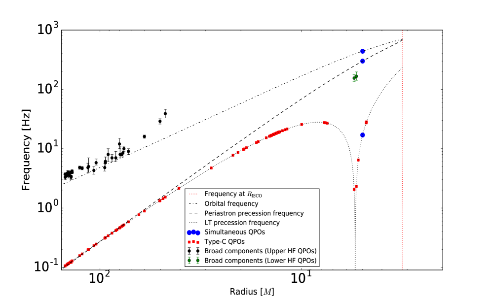
In our paper, we have considered a non-zero NUT parameter, which makes the results from three $a/M$ measurement methods consistent with each other. An important point is, even for a non-zero NUT parameter, our results could qualitatively explain the pairs of simultaneous LFQPO and HFQPO by RPM (like in Fig. 5 of Motta et al. motta40 ). We show it in our Fig. 2. However, a difference with Fig. 5 of Motta et al. motta40 is, we consider Motta et al.’s upper HFQPOs as lower HFQPOs, and Motta et al.’s lower HFQPOs as upper HFQPOs. Our this assumption is not worse than Motta et al.’s assumption, because there is no independent way to find out which HFQPOs are lower ones, and which are upper ones (when they are not simultaneously observed). Note that in both figures (our Fig. 2 and Motta et al.’s Fig. 5), the data points and model curves have similar trends, although the model curves do not quantitatively describe the data points well either in Motta et al.’s case or in our case, possibly due to systematics related to additional physical complexities (see Sec.VI). Nevertheless, the qualitative matching between the model and the data, shown in both the figures, tentatively supports the RPM method.

However, the LT precession frequency can change sign for a non-zero NUT parameter, as one moves outwards from the collapsed object. This implies the same absolute value of the LT precession frequency at three different radius values (see Fig. 2). Note that we take the absolute value, because a negative frequency only implies the opposite direction, which is not important for our purpose. Therefore, applying the similar method we followed to solve Eqs. (18), two more sets of parameter values could be obtained from the solution of the following equations:

$$\nu_{\phi}^{\rm KTN}=440~{}{\rm Hz};\,\,\nu_{\rm per}^{\rm KTN}=300~{}{\rm Hz};\,\,\,\,\nu_{\rm LT}^{\rm KTN}=-17~{}{\rm Hz}.$$ (19)

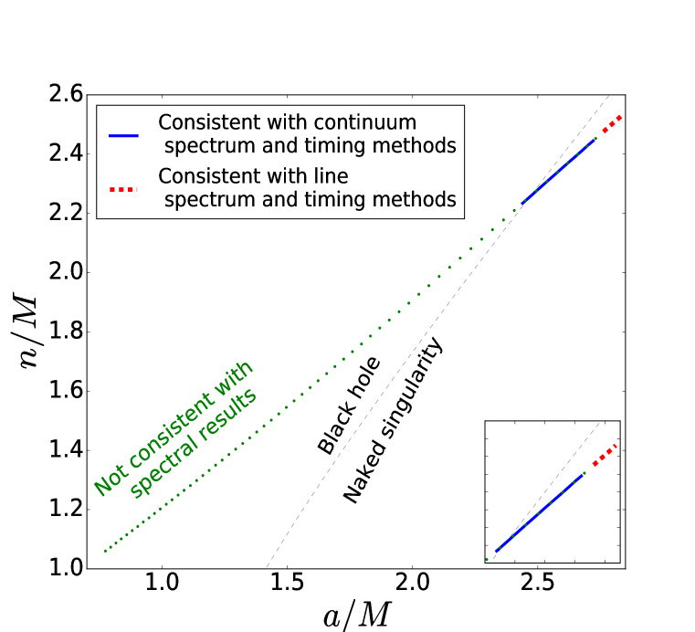
It is clearly seen from Fig. 3, that, for the second set of the parameter values, no range of $n/M$ and $a/M$ values for GRO J1655–40 is allowed by all the three methods (RPM, line spectrum and continuum spectrum). Therefore, we can rule out this solution. The third set of parameter values do not come out as real and physical for the observed frequencies of the three simultaneous QPOs. Therefore, as the second solution is not consistent with the three different spin measurement methods, and the third solution does not exist, we do not consider these additional sets of parameter values. Thus, only the first solution (for the ‘positive’ LT precession frequency), which has been discussed in Sec.IV, is acceptable.

Figure 3: The NUT parameter ($n/M$) versus the spin parameter ($a/M$) space, which is divided into a black hole region and a naked singularity region by the black dashed line. The $n/M$ versus $a/M$ constraints for GRO J1655–40 are given by (1) the green dotted curve (using only the RPM timing method), (2) the red dotted curve (using the RPM timing and line spectrum methods, and (3) the blue solid curve (using the RPM timing and continuum spectrum methods). A zoomed version of the latter two is shown in the inset for clarity. This figure (for the second set of the parameter values; see Sec. V) shows that there is no range of $n/M$ and $a/M$ values for GRO J1655–40 allowed by all the three methods, unlike Fig. 1.

VI Conclusion and Discussion

It has been shown that $a/M\approx 2.12-2.21$ and $n/M\approx 1.86-1.93$ are consistent with all the three methods. These ranges imply that the collapsed object in GRO J1655–40 is a naked singularity (Fig. 1). Besides, the lower limit $1.86$ of $n/M$ implies the existence of the gravitomagnetic monopole. While this is not a direct detection of such a monopole, the indication is strong within our paradigm for the following reasons. Recall that the three methods gave widely different constraints on $a/M$ ($\approx 0.286\pm 0.003$ motta40 ; $\approx 0.90-0.99$ Reisetal2009 ; $\approx 0.65-0.75$ sha ). With only one additional parameter (i.e., the NUT parameter $n/M$), it might be possible to make the constraints from two of these methods consistent with each other. We have attempted this separately for two joint methods: (1) RPM and line spectrum method, and (2) RPM and continuum spectrum method; and obtained combined parameter constraints for each of these cases. While this is not unexpected (as we have used an additional parameter $n$), the combined constraint on $M$ being consistent with an independently measured mass value for each of the joint methods already shows the reliability of our approach. But the main strength of our results is, we also find that the combined constraints on each of $n/M$ and $a/M$ from these two joint methods are largely overlapping with each other. This cannot be a result of fine-tuning, as with just one additional parameter ($n$), it is not possible to fine-tune and make three different results from three independent methods consistent with each other. Hence, the fact that we have found consistent $a/M$ and $n/M$ ranges from all three methods by invoking just one additional parameter ($n$) points to the non-zero $n$ values for GRO J1655–40, and hence suggests the existence of the gravitomagnetic monopole in nature. This is further confirmed by the consistent ranges of $r_{\rm qpo}/M$ ($\approx 4.99-5.02$) and $M$ ($\approx 6.79-6.83M_{\odot}$) for the methods, as well as the consistency of this $M$ range with an independently measured value ($[6.3\pm 0.5]M_{\odot}$; Greeneetal2001 ). This confirmation also provides a new way to measure the NUT parameter, even when only two $a/M$ measurement methods are available for a BHXB. It should be noted that like $a/M$, the value of $n/M$ can be different for different objects and a high $n/M$ value inferred for one object in this paper does not mean that every object will have a high $n/M$ value. The value of $n/M$ can even be very close to zero for some objects. But the inferred significantly non-zero $n/M$ value for even one object could strongly suggest the existence of gravitomagnetic monopole in nature. Our new technique also makes the black hole spin measurement methods more reliable.

Here we note that the ‘extra angular momentum’ bon makes the Taub-NUT metric singular (coordinate singularity) at $\theta=\pi$, which is a ‘Dirac string singularity’ rs2 . Misner mis wanted to present an entirely nonsingular cosmological model (homogeneous and anisotropic) with the Taub-NUT metric, which contains the closed spacelike hypersurfaces (but no matter), and this made this metric singularity-free. Ramaswamy and Sen rs ; rs2 pointed out that the presence of NUT parameter requires that either the Taub-NUT metric can be singular (not the curvature) or the spacetime contains closed timelike curves. Since, in this paper, we have also included a possibility of the KTN ‘naked singularity’, we do not require the ‘singularity-free spacetime’ to interpret our results. This means that the ‘closed timelike curves’ are not required for our interpretation.

Note that we have not fit the observed spectra with KTN spectral models, because such models are not currently available. Instead, for the purpose of $a/M$ estimation, we have used $r_{\rm ISCO}$ and the gravitational redshift at $r_{\rm ISCO}$ as proxies for the details of continuum spectrum and line spectrum respectively. As argued in this paper, the use of these proxies is reasonable, although such a use can introduce some systematics in the inferred parameter ranges. However, given that the inferred $n/M$ range ($\approx 1.86-1.93$) is significantly away from $n/M=0$ (see Fig. 1), the inferred non-zero $n/M$ values cannot be caused by these systematics. Besides, $n/M=0$ gives three widely different $a/M$ ranges from three different methods for GRO J1655–40, as discussed earlier. Therefore, this paper presents the first significant observational indication of the gravitomagnetic monopole, which, even though is not a direct detection, can have an exciting impact on fundamental physics and astrophysics. However, although the allowed $n/M$ versus $a/M$ range is in the naked singularity region (Fig. 1), it is close to the border of the black hole region, and hence the indication of a naked singularity is only suggestive.

Finally, note that our inference of a non-zero NUT parameter could be correct for our assumption, i.e., the three existing methods of black hole spin measurements are reliable. However, one or more of these methods may not be entirely reliable due to additional physical complexities. Some of these complexities may be due to the following reasons (e.g., kraw discusses how difficult it is to test the Kerr metric with X-ray observations). (1) The continuum X-ray spectrum method assumes that the thin disk emission can be fully separated from emissions from other X-ray components, which may not be correct. (2) Spectral methods also assume that the black hole’s spin is aligned with the inner disk angular momentum vector, which is not necessarily true ChakrabortyBhattacharyya2017 . (3) The relativistic precession model assumes that particles in the accretion disk travel on exact geodesic orbits, and neglects important physics such as radiation physics, viscosity, magnetic fields that could affect the motion of material in the disk. While there is a possibility that such systematic uncertainties could explain the three different ranges of spin values obtained from three methods for $n=0$, such a level of unreliability of the methods would make many of the current black hole studies doubtful and could impact the plans of X-ray observations of BHXBs with future space missions (Sec.II).

Appendix A Fundamental frequencies in a general stationary and axisymmetric spacetime

Let us consider a general stationary and axisymmetric spacetime as

$$ds^{2}=g_{tt}dt^{2}+2g_{t\phi}d\phi dt+g_{\phi\phi}d\phi^{2}+g_{rr}dr^{2}+g_{\theta\theta}d\theta^{2},$$ (20)

where $g_{\mu\nu}=g_{\mu\nu}(r,\theta)$. In this spacetime, the proper angular momentum ($l$) of a test particle can be defined as:

$$l=-\frac{g_{t\phi}+\Omega_{\phi}g_{\phi\phi}}{g_{tt}+\Omega_{\phi}g_{t\phi}},$$ (21)

where, $\Omega_{\phi}$ is the orbital frequency of the test particle. $\Omega_{\phi}$ is defined as don

$$\Omega_{\phi}\equiv 2\pi\nu_{\phi}=\frac{d\phi/d\tau}{dt/d\tau}=\frac{d\phi}{dt}=\frac{-g_{t\phi}^{\prime}\pm\sqrt{g_{t\phi}^{\prime 2}-g_{tt}^{\prime}g_{\phi\phi}^{\prime}}}{g_{\phi\phi}^{\prime}}\mid_{r={\rm constant},\theta\rightarrow\pi/2},$$ (22)

where the prime denotes the partial differentiation with respect to $r$. The general expressions for calculating the radial ($\nu_{r}$) and vertical ($\nu_{\theta}$) epicyclic frequencies are don

$$\nu_{r}^{2}=\frac{(g_{tt}+\Omega_{\phi}g_{t\phi})^{2}}{2(2\pi)^{2}~{}g_{rr}}\left[\partial_{r}^{2}\left({g_{\phi\phi}}/{Y}\right)+2l~{}\partial_{r}^{2}\left({g_{t\phi}}/{Y}\right)+l^{2}~{}\partial_{r}^{2}\left({g_{tt}}/{Y}\right)\right]|_{r={\rm constant},\theta\rightarrow\pi/2}$$

(23)

and

$$\nu_{\theta}^{2}=\frac{(g_{tt}+\Omega_{\phi}g_{t\phi})^{2}}{2(2\pi)^{2}~{}g_{\theta\theta}}\left[\partial_{\theta}^{2}\left({g_{\phi\phi}}/{Y}\right)+2l~{}\partial_{\theta}^{2}\left({g_{t\phi}}/{Y}\right)+l^{2}~{}\partial_{\theta}^{2}\left({g_{tt}}/{Y}\right)\right]|_{r={\rm constant},\theta\rightarrow\pi/2}$$

(24)

respectively, and $Y$ is defined as

$$Y=g_{tt}g_{\phi\phi}-g_{t\phi}^{2}.$$ (25)

Gravitational redshift

The general expression of gravitational redshift ($z$) in an axisymmetric and stationary spacetime can be obtained from mtw ; lum

$$Z=1+z=(-g_{tt}-2\Omega_{\phi}g_{t\phi}-\Omega_{\phi}^{2}g_{\phi\phi})^{-\frac{1}{2}}.$$ (26)

Now, substituting the expressions of metric components ($g_{\mu\nu}$) and the orbital frequency ($\Omega_{\phi}$) in Eq. (26), one can derive the expression of $Z$ of a particular axisymmetric and stationary spacetime, i.e., KTN, Kerr, NUT, etc. We discuss these in Sec. III.

Acknowledgements : We thank the referee for the constructive comments and valuable suggestions. One of us (C. C.) also thanks T. Baug for some useful discussions. C. C. gratefully acknowledges support from the National Natural Science Foundation of China (NSFC), Grant No. : 11750110410.

References

- (1) P. A. M. Dirac, Proc. R. Soc. Lond. A 133, 60 (1931)
- (2) M. N. Saha, Indian Journal of Physics X, 141 (1936)
- (3) A. Zee, Phys. Rev. Lett. 55, 2379 (1985)
- (4) E. Newman, L. Tamburino, T. Unti, J. Math. Phys. 4, 915 (1963)
- (5) V. Kagramanova, B. Ahmedov, Gen. Relativ. Gravit. 38, 823 (2006)
- (6) D. Bini, C. Cherubini, R. T. Jantzen, B. Mashhoon, Class. Quantum Grav. 20, 457 (2003)
- (7) S. Ramaswamy, A. Sen, Phys. Rev. Lett. 57, 1088 (1986)
- (8) M. Demianski, E.T. Newman, Bull. Acad. Pol. Sci., Ser. Sci. Math. Astron. Phys. 14, 653 (1966)
- (9) W. B. Bonnor, Proc. Camb. Phil. Soc. 66, 145 (1969)
- (10) J. S. Dowker, Gen. Rel. Grav. 5, 603 (1974)
- (11) S. Ramaswamy, A. Sen, J. Math. Phys. (N.Y.) 22, 2612 (1981)
- (12) M. Mueller, M. J. Perry, Class. Quantum Grav. 3, 65 (1986)
- (13) D. Lynden-Bell, M. Nouri-Zonoz, Rev. Mod. Phys. 70, 427 (1998)
- (14) V. Kagramanova, J. Kunz, E. Hackmann, C. Lämmerzahl, Phys. Rev. D81, 124044 (2010)
- (15) R. Kerr, Phys. Rev. Lett. 11, 237 (1963)
- (16) J. G. Miller, J. Math. Phys. 14, 486 (1973)
- (17) C. Chakraborty, P. Kocherlakota, M. Patil, S. Bhattacharyya, P. S. Joshi, A. Królak, Phys. Rev. D 95, 084024 (2017)
- (18) J. M. Miller, ARAA 45, 441 (2007)
- (19) R. A., Remillard, J. E. McClintock, ARAA 44, 49 (2006)
- (20) T. M. Belloni, L. Stella, Space Science Reviews 183, 43 (2014)
- (21) S. E. Motta, T. M. Belloni, L. Stella, T. Munoz-Darias, R. Fender, Mon. Not. R. Astron. Soc. 437, 2554 (2014)
- (22) C. S. Reynolds, M. A. Nowak, Phys. Rep. 377, 389 (2003)
- (23) R. C. Reis, A. C. Fabian, R. R. Ross, J. M. Miller, Mon. Not. R. Astron. Soc. 395, 1257 (2009)
- (24) T. Fragos, J. E. McClintock, Astrophys J. 800, 17 (2015)
- (25) T. M. Belloni, A. Sanna, M. Méndez, Mon. Not. R. Astron. Soc. 426, 1701 (2012)
- (26) L. Stella, M. Vietri, Astrophys J., 492, L59 (1998)
- (27) L. Stella, M. Vietri, Phys. Rev. Lett. 82, 17 (1999)
- (28) J. Greene, C. D. Bailyn, J. A. Orosz, Astrophys. J. 554, 1290 (2001)
- (29) M. E. Beer, P. Podsiadlowski, Mon. Not. R. Astron. Soc. 331, 351 (2002)
- (30) A. Ingram, M. van der Klis, M. Middleton, C. Done, D. Altamirano, L. Heil, P. Uttley, M. Axelsson, Mon. Not. R. Astron. Soc. 461, 1967 (2016)
- (31) J. M. Miller, J. Homan, Astrophys J. 618, L107 (2005)
- (32) J. D. Schnittman, J. Homan, J. M. Miller, Astrophys J. 642, 420 (2006)
- (33) C. Chakraborty, S. Bhattacharyya, Mon. Not. R. Astron. Soc. 469, 3062 (2017)
- (34) R. Shafee, J. E. McClintock, R. Narayan, S. W. Davis, L.-X. Li, R. A. Remillard, Astrophys. J. 636, L113 (2006)
- (35) C. Chakraborty, Eur. Phys. J. C74, 2759 (2014)
- (36) A. T. Okazaki, S. Kato, J. Fukue, PASJ 39, 457 (1987)
- (37) S. Kato, PASJ 42, 99 (1990)
- (38) S. Chandrasekhar, The Mathematical Theory of Black Holes, Oxford (1992)
- (39) C. Chakraborty, P. Kocherlakota, P. S. Joshi, Phys. Rev. D 95, 044006 (2017)
- (40) S-W. Wei, Y-X. Liu, C-E Fu, K. Yang, JCAP 10 (2012) 053
- (41) P. S. Joshi, D. Malafarina, IJMPD 20, 2641 (2011)
- (42) C. W. Misner, J. Math. Phys. 4, 924 (1963)
- (43) H. Krawczynski, Gen. Relativ. Gravit. 50, 100 (2018)
- (44) D. D. Doneva, S. S. Yazadjiev, N. Stergioulas, K. D. Kokkotas, T. M. Athanasiadis, Phys. Rev. D 90, 044004 (2014)
- (45) C. W. Misner, K. S. Thorne, J. A. Wheeler, Gravitation, W. H Freeman Company, (1973)
- (46) J.-P. Luminet, Astron. and Astrophys. 75, 228 (1979)