Distributed Algorithms Made Secure:
A Graph Theoretic Approach

Abstract

In the area of distributed graph algorithms a number of network’s entities with local views solve some computational task by exchanging messages with their neighbors. Quite unfortunately, an inherent property of most existing distributed algorithms is that throughout the course of their execution, the nodes get to learn not only their own output but rather learn quite a lot on the inputs or outputs of many other entities. This leakage of information might be a major obstacle in settings where the output (or input) of network’s individual is a private information (e.g., distributed networks of selfish agents, decentralized digital currency such as Bitcoin).

While being quite an unfamiliar notion in the classical distributed setting, the notion of secure multi-party computation (MPC) is one of the main themes in the Cryptographic community. The existing secure MPC protocols do not quite fit the framework of classical distributed models in which only messages of bounded size are sent on graph edges in each round. In this paper, we introduce a new framework for secure distributed graph algorithms and provide the first general compiler that takes any “natural” non-secure distributed algorithm that runs in $r$ rounds, and turns it into a secure algorithm that runs in $\widetilde{O}(r\cdot D\cdot\mathsf{poly}(\Delta))$ rounds where $\Delta$ is the maximum degree in the graph and $D$ is its diameter. A “natural” distributed algorithm is one where the local computation at each node can be performed in polynomial time. An interesting advantage of our approach is that it allows one to decouple between the price of locality and the price of security of a given graph function $f$. The security of the compiled algorithm is information-theoretic but holds only against a semi-honest adversary that controls a single node in the network.

This compiler is made possible due to a new combinatorial structure called private neighborhood trees: a collection of $n$ trees $T(u_{1}),\ldots,T(u_{n})$, one for each vertex $u_{i}\in V(G)$, such that each tree $T(u_{i})$ spans the neighbors of $u_{i}$ without going through $u_{i}$. Intuitively, each tree $T(u_{i})$ allows all neighbors of $u_{i}$ to exchange a secret that is hidden from $u_{i}$, which is the basic graph infrastructure of the compiler. In a $(\mbox{\tt d},\mbox{\tt c})$-private neighborhood trees each tree $T(u_{i})$ has depth at most d and each edge $e\in G$ appears in at most c different trees. We show a construction of private neighborhood trees with $\mbox{\tt d}=\widetilde{O}(\Delta\cdot D)$ and $\mbox{\tt c}=\widetilde{O}(D)$, both these bounds are existentially optimal.

1 Introduction

In distributed graph algorithms (or network algorithms) a number of individual entities are connected via a potentially large network. Starting with the breakthrough by Awerbuch et al. [AGLP89], and the seminal work of Linial [Lin92], Peleg [Pel00] and Naor and Stockmeyer [NS95], the area of distributed graph algorithms is growing rapidly. Recently, it has been receiving considerably more theoretical and practical attention motivated by the spread of multi-core computers, cloud computing, and distributed databases. We consider the standard synchronous message passing model (the ${\mathsf{CONGEST}}$ model) where in each round $O(\log n)$ bits can be transmitted over every edge where $n$ is the number of entities.

The common principle underlying all distributed graph algorithms (regardless of the model specification) is that the input of the algorithm is given in a distributed format. Consequently the goal of each vertex is to compute its own part of the output, e.g., whether it is a member of a computed maximal independent set, its own color in a valid coloring of the graph, its incident edges in the minimum spanning tree, or its chosen edge for a maximal matching solution. In most distributed algorithms, throughout execution, vertices learn much more than merely their own output but rather collect additional information on the input or output of (potentially) many other vertices in the network. This seems inherent in many distributed algorithms, as the output of one node is used in the computation of another. For instance, most randomized coloring (or MIS) algorithms [Lub86, BE13, BEPS16, HSS16, Gha16, CPS17] are based on the vertices exchanging their current color with their neighbors in order to decide whether they are legally colored.

In cases where the data is sensitive or private, these algorithms may raise security concerns. To exemplify this point, consider the task of computing the average salary in a distributed network. This is a rather simple distributed task: construct a BFS tree and let the nodes send their salary from the leaves to the root where each intermediate node sends to its parent in the tree, the sum of all salaries received from its children. While the output goal has been achieved, privacy has been compromised as intermediate nodes learn more information regarding the salaries of their subtrees. Additional motivation for secure distributed computation includes private medical data, networks of selfish agents with private utility functions, and decentralized digital currencies such as the Bitcoin.

The community of distributed graph algorithms is commonly concerned with two primary challenges, namely, locality (i.e., communication is only performed between neighboring nodes) and congestion (i.e., communication links have bounded bandwidth). Security is usually not specified as a desired requirement of the distributed algorithm and the main efficiency criterion is the round complexity (while respecting bandwidth limitation).

Albeit being a rather virgin objective in the area of distributed graph algorithms, the notion of security in multi-party computation (MPC) is one of the main themes in the Cryptographic community. Broadly speaking, secure MPC protocols allow parties to jointly compute a function $f$ of their inputs without revealing anything about their inputs except the output of the function. There has been tremendous work on MPC protocols, starting from general feasibility results [Yao82, GMW87, BGW88, CCD88] that apply to any functionality to protocols that are designed to be extremely efficient for specific functionalities [BNP08, BLO16]. There is also a wide range of security notions: information-theoretic security or security that is based on computational assumptions, the adversary is either semi-honest or malicious and in might collude with several parties.

Most MPC protocols are designed for the clique networks where every two parties have a secure channel between them. The works that do consider general graph topologies usually take the following framework. For a given function $f$ of interest, design first a protocol for securely computing $f$ in the simpler setting of a clique network, then “translate” this protocol to any given graph $G$. Although this framework yields protocols that are secure in the strong sense (e.g., handling collusions and a malicious adversary), they do not quite fit the framework of distributed graph algorithms, and simulating these protocols in the ${\mathsf{CONGEST}}$ model results in a large overhead in the round complexity. It is important to note that the blow-up in the number of rounds might occur regardless of the security requirement; for instance, when the desired function $f$ is non-local, its distributed computation in general graphs might be costly with respect to rounds even in the insecure setting. In the lack of distributed graph algorithms for general graphs that are both secure and efficient compared to their non-secure counterparts, we ask:

How to design distributed algorithms that are both efficient (in terms of round complexity) and secure (where nothing is learned but the desired output)?

We address this challenge by introducing a new framework for secure distributed graph algorithms in the ${\mathsf{CONGEST}}$ model. Our approach is different from previous secure algorithms mentioned above and allows one to decouple between the price of locality and the price of security of a given function $f$. In particular, instead of adopting a clique-based secure protocol for $f$, we take the best distributed algorithm ${\mathcal{A}}$ for computing $f$, and then compile ${\mathcal{A}}$ to a secure algorithm ${\mathcal{A}}^{\prime}$. This compiled algorithm respects the same bandwidth limitations relies on no setup phase nor on any computational assumption and works for (almost) any graph. The price of security comes as an overhead in the number of rounds. Before presenting the precise parameters of the secure compiler, we first discuss the security notion used in this paper.

Our Security Notion.

Consider a (potentially insecure) distributed algorithm ${\mathcal{A}}$. Intuitively, we say that a distributed algorithm ${\mathcal{A}}^{\prime}$ securely simulates ${\mathcal{A}}$ if (1) both algorithms have the exact same output for every node (or the exact same output distribution if the algorithm is randomized) and (2) each node learns “nothing more” than its final output. This strong notion of security is known as “perfect privacy” - which provides pure information theoretic guarantees and relies on no computational assumptions. The perfect privacy notion is formalized by the existence of an (unbounded) simulator [BGW88, Gol09, Can00, AL17], with the following intuition: a node learns nothing except its own output $y$, from the messages it receives throughout the execution of the algorithm, if a simulator can produce the same output distribution while receiving only $y$ and the graph $G$.

Assume that one of the nodes in the network is an “adversary” that is trying to learn as much as possible from the execution of the algorithm. Then the security notion has some restrictions on the operations the adversary is allowed to perform: (1) The adversary is passive and only listens to the messages but does not deviate from the prescribed protocol; this is known in the literature as semi-honest security. (2) The adversary is not allowed to collude with other nodes in the network. As will be explained next, if the vertex connectivity of the graph is two, then this is the strongest adversary that one can consider. (3) The adversary gets to see the entire graph. That is, in this framework, the topology of the graph $G$ is not considered private and is not protected by the security notion. The private bits of information that are protected by our compiler are: the inputs of the nodes (e.g., color) and the randomness chosen during the execution of the algorithm; as a result, the outputs of the nodes are private (see Definition 1 for precise details).

A Stronger Adversary: From Cliques to General Topology.

The goal of this paper is to lay down the groundwork, especially the graph theoretic infrastructures for secure distributed graph algorithms. As a first step towards this goal, we consider the largest family of graphs for which secure computation can be achieved in the perfect secure setting. This is precisely the family of two-vertex connected graphs.

Handling this wide family of graphs naturally imposes restrictions on the power of the adversary that one can consider. In particular, we cannot hope to handle that standard adversary assumed in the MPC literature, which colludes with $\Omega(n)$ other parties. A natural limit on the adversarial collusion is the vertex connectivity of the graph. Indeed, if the graph is only $t$-vertex connected, then an adversary that colludes with $t$ nodes can receive all messages from one part of the graph to the other. That is, security for such a graph will imply a secure two-party computation, where each party simulates one connected component of the graph. Such two-party secure protocols where shown to be impossible for merely any interesting function [Kus89]. Thus, for 2-vertex connected graphs, one cannot achieve a secure simulation with an adversary that colludes with more than a node. Moreover, the works of [Dol82] combined with [DDWY93] show that if the adversary is malicious and colludes with $t$ nodes then graph must be $(2t+1)$ connected for security to hold.

We believe that the framework provided in this paper, and the private neighborhood trees in particular, serve the basis for stronger security guarantees in the future, for highly connected graphs.

1.1 Our Results

Our end result is the first general compiler that can take any “natural” (possibly insecure) distributed algorithm to one that has perfect security. A “natural” distributed algorithm is one where the local computation at each node can be performed in polynomial time. Through the paper, the $\widetilde{O}(\cdot)$ notation hides poly-logarithmic terms in the number of vertices $n$. Recall, that $G$ is 2-vertex connected (or bridgeless) if for all $u\in V$ the graph $G^{\prime}=(V\setminus\{u\},E)$ is connected.

Theorem 1 (Secure Simulation, Informal).

Let $G$ be a 2-vertex connected $n$-vertex graph with diameter $D$ and maximal degree $\Delta$. Let $\mathcal{A}$ be a natural distributed algorithm that runs on $G$ in $r$ rounds. Then, $\mathcal{A}$ can be transformed to an equivalent algorithm $\mathcal{A}^{\prime}$ with perfect privacy which runs in $\widetilde{O}(rD\cdot\mathsf{poly}(\Delta))$ rounds.

We note that our compiler works for any distributed algorithm rather than only on natural ones. The number of rounds will be proportional to the space complexity of the internal computation functions of the distributed algorithm (an explicit statement for any algorithm can be found in Remark 1).

This quite general framework is made possible due to fascinating connections between “secure cryptographic definitions” and natural combinatorial graph properties. Most notably is a combinatorial structure that we call private neighborhood trees. Roughly speaking, a private neighborhood tree of a 2-vertex connected graph $G=(V,E)$ is a collection of $n$ trees, one per node $u_{i}$, where each tree $T(u_{i})\subseteq G\setminus\{u_{i}\}$ contains all the neighbors of $u_{i}$ but does not contain $u_{i}$. Intuitively, the private neighborhood trees allow all neighbors $\Gamma(u_{i})$ of all nodes $u_{i}$ to exchange a secret without $u_{i}$. Note that these covers exist if and only if the graph is 2-vertex connected. We define a $(\mbox{\tt d},\mbox{\tt c})$-private neighborhood trees in which each tree $T(u_{i})$ has depth at most d and each edge belongs to at most c many trees. This allows the distributed compiler to use all trees simultaneously in $\widetilde{O}(\mbox{\tt d}+\mbox{\tt c})$ rounds, by employing the random delay approach [LMR94, Gha15].

Theorem 2 (Private Neighborhood Trees).

Every $2$-vertex connected graph with diameter $D$ and maximum degree $\Delta$ has a $(\mbox{\tt d},\mbox{\tt c})$-private neighborhood trees with $\mbox{\tt d}=\widetilde{O}(D\cdot\Delta)$ and $c=\widetilde{O}(D)$.

Our secure compiler assumes that the nodes in the graph know the private neighborhood trees. That is, each node knows its parent in the trees it participates in. Thus, in order for the whole transformation to work, the network needs to run a distributed algorithm to learn the cycle cover. This can be achieved by performing a prepossessing phase to compute the private trees and then run the distributed algorithm.

Since the barrier of [Kus89] can be extended to a cycle graph, the linear dependency in $D$ in the round complexity of our compiler is unavoidable.

The flow of our constructions is summarized in Figure 1.

Figure 1: An illustrated summary of our results.

1.2 Applications for Known Distributed Algorithms

Theorem 1 enables us to compile almost all of the known distributed algorithms to a secure version of them. It is worth noting that deterministic algorithms for problems in which the nodes do not have any input cannot be made secure by our approach since these algorithms only depend on the graph topology which we do not try to hide. Our compiler is meaningful for algorithms where the nodes have input or for randomized algorithms which define a distribution over the output of the nodes. For instance, the randomized coloring algorithms (see, e.g., [BE13]) which sample a random legal coloring of the graph can be made secure. Specifically, we get a distributed algorithm that (legally) colors a graph (or computes a legal configuration, in general), while the information that each node learns at the end is as if a centralized entity ran the algorithm for the entire network, and revealed each node’s output privately (i.e., revealing $v$ the final color of $v$).

Our approach captures global (e.g., MST) as well as many local problems [NS95]. The MIS algorithm of Luby [Lub86] along with our compiler yields $\widetilde{O}(D\cdot\mathsf{poly}(\Delta))$ secure algorithm according to the notion described above. Slight variations of this algorithm also give the $O(\log n)$-round $(\Delta+1)$-coloring algorithm (e.g., Algorithm 19 of [BE13]). Combining it with our compiler, we get a secure $(\Delta+1)$-coloring algorithm with round complexity of $\widetilde{O}(D\cdot\mathsf{poly}(\Delta))$. Using the Matching algorithm of Israeli and Itai [II86] we get an $\widetilde{O}(D\cdot\mathsf{poly}(\Delta))$ secure maximal matching algorithm. Finally, another example comes from distributed algorithms for the Lovász local lemma (LLL) which have received much attention recently [BFH⁺16, FG17, CP17] for the class of bounded degree graphs. Using [CPS17], most of these (non-secure) algorithms for defective coloring, frugal coloring, and list vertex-coloring can be made secure within $\widetilde{O}(D)$ rounds.

1.3 Related Work

There is a long line of research on secure multiparty computation. The most general results are [Yao82, GMW87, BGW88, CCD88] which provide a protocol for computing any function $f(x_{1},\ldots,x_{n})$ over $n$ inputs. The significance of these results is that they work for any function and provide strong security (either assuming computational assumptions, or information-theoretic as is considered in this work). More specifically, these results can tolerate the adversary colluding with $t$ nodes as long as $t<n/2$ and achieve security in the semi-honest model. If the adversary is malicious (i.e., she can deviate from the prescribed protocol) then the protocols can handle $t<n/3$. These general results assume that every two parties have a secure direct channel between them, that is, they assume that the interaction pattern is a clique.

General Graph Topologies.

As opposed to general MPC, there are not many protocols that work for general graph interaction patterns. The works of [HIJ⁺16, HIJ⁺17] provide secure protocols for any function $f$ and for any graph pattern, however, they have a few drawbacks. First, they both assume some form of a setup phase (recall that our solution assumes no such setup). The work of [HIJ⁺16] assumes a setup of correlated randomness and provides several protocols with information-theoretic security. Even the most efficient protocol (one for symmetric functions) must send more than $n^{2}$ bits on each edge. In the CONGEST model, this would take $n^{2}/\log n$ rounds which is not an interesting regime for this model (for other functions the communication complexity is much worse). The work of [HIJ⁺17] assumes a public-key infrastructure (PKI) setup together with a common random string, and moreover provides only solutions based on (heavy) computational assumptions. More importantly, the number of rounds is not a parameter they optimize and will be at least $O(n^{2})$ even for simple functions. Such protocols were also implicitly considered in [GGG⁺14, BGI⁺14] but suffer from similar drawbacks.

MPC with Locality Constraints.

Other MPC works study protocols with small locality, that is, that parties communicate only with a small number of other parties. The work of [BGT13] (followed by [CCG⁺15]) provides a secure MPC protocol for general functions where for $n$ parties each party is only required to communicate with at most $\mathsf{polylog}(n)$ other parties using $\mathsf{polylog}(n)$ rounds, where in each round messages are of size $\mathsf{poly}(n)$. Their protocols assume computation assumptions and a setup phase. Moreover, we stress that they still require a fully connected network, and then parties communicate with a small number of dynamically chosen parties, but with very large messages (compared to the $\log n$ bound in our model). On the positive side, they achieve a strong security notation where the adversary can collude with up to about $n/3$ nodes.

MPC for Bounded Degree Graphs.

The works of [GO08, CGO10] consider MPC protocols for bounded degree graphs. Except for the graph restriction, they consider arbitrary interaction pattern, information-theoretic security and no setup phase (similar to our setting). They provide a protocol for computing any function $f$ while “giving up” on security for some nodes (i.e., the adversary might learn the private inputs of these nodes). While they have some restrictions on the adversary, their security notion is stronger than ours (as we do not allow collusions). However, their protocol is not round nor bandwidth efficient with respect to our parameters. They simulate the general MPC protocol of [BGW88], by replacing each message sent from player $i$ to player $j$, one-by-one, with a distributed broadcast protocol that takes more than $n$ rounds by itself. Thus, the overall protocols will require at least $n^{2}$ rounds and enters the uninteresting regime of parameters for the CONGEST model.

The Key Differences to Our Approach.

Our approach is quite different from the algorithms mentioned above. In particular, instead of taking some function $f$ and trying to build the best secure protocol for it, our compiler takes the best distributed algorithm for computing $f$, and then compiles it to a secure one. This makes us competitive, in terms of the number of rounds, with the non-secure distributed algorithm. In the MPC approach, it is harder to decouple between the price of locality and the price of security as adopting a clique-protocol for computing a function $f$ to a general graph might blow up the number of rounds, regardless of the security constraint. One exception is the work of [KTW07] who showed how to compile a distributed algorithm for a specific task of Belief Propagation to a secure one. The compiler is designed specifically for this task and does not work for others. Moreover, the security that is achieved is based on computational assumption and specifically public-key encryption with additional properties.

Finally, we note that a compiler that works for even a weaker adversary was proposed in [PY18]. In their setting, the adversary can listen to the messages of a single edge where in our setting the adversary listens to all messages received by a single node. Thus, the adversary gets messages from $\Delta$ different edges in addition to getting the private randomness chosen by the node itself.

2 Our Approach and Techniques

We next describe the high-level ideas of our secure compiler. In section 2.1, we describe how the secure computation in the distributed setting boils down into a novel graph theoretic structure, namely, private neighborhood trees. The construction of private trees is shown in Section 4.

2.1 From Security Requirements to Graph Structures

In this section, we give an overview of the construction of a secure compiler and begin by showing how to compile a single round distributed algorithm into a secure one. This single-round setting already captures most of the challenges of the compiler. At the end of the section, we describe the additional ideas required for generalizing this to arbitrary $r$-round algorithms.

Secure Simulation of a Single Round.

Let $G$ be an $n$-vertex graph with maximum degree $\Delta$, and for any node $u$ let $\sigma_{u}$ be its initial state (including its ID, and private input). Any single round algorithm can be described by a function $f$ that maps the initial state $\sigma_{u}$ of $u$ and the messages $m_{1},\ldots,m_{\Delta}$ received from its neighbors to the output of the algorithm for the node $u$.

As a concrete running example, let ${\mathcal{A}}$ be a single round algorithm that verifies vertex coloring in a graph. In this algorithm, the initial state of a node includes a color $c_{u}$, and nodes exchange their color with their neighbors and output $1$ if and only if all of their neighbors are colored with a color that is different from $c_{u}$. It is easy to see that in this simple algorithm, the nodes learn more than the final output of the algorithm, namely, they learn the color of their neighbors. Our goal is to compile this algorithm to a secure one, where nothing is learned expect the final output. In particular, where nodes do not learn the color of any other node in the network. This fits the model of Private Simultaneous Messages (PSM) that we describe next. We stress that other MPC protocols might be suitable here as well (e.g., [Yao82, GMW87, BGW88]), however, the star topology of PSM model makes the best fit in terms of simplicity and parameters.

The PSM model was introduced by Feige, Kilian and Naor [FKN94] (and later generalized by [IK97]) as a “minimal” model of MPC for securely computing a function $f$. In this model, there are $k$ clients that hold inputs $x_{1},\ldots,x_{k}$ which are all connected to a single server (i.e., a star topology). The clients share private randomness $R$ that is hidden from the server. The goal is for the server to compute $f(x_{1},\ldots,x_{k})$ while learning “nothing more” but this output. The protocol consists of a single round where each client $i$ sends a message to the server that depends on its own input $x_{i}$ and the randomness $R$. The server, using these messages, computes the final output $f(x_{1},\ldots,x_{k})$. In [FKN94], it was shown that any function $f$ admits such a PSM protocol with information-theoretic privacy. The complexity measure of the protocol is the size of the messages (and shared randomness) which are exponential in the space complexity of the function $f$ (see Definition 2 and Theorem 5 for precise details).

Turning back to our single round distributed algorithm ${\cal A}$, the secure simulation of ${\cal A}$ can be based on the PSM protocol for securely computing the function $f$, the function that characterizes algorithm ${\mathcal{A}}$. In this view, each node $u$ in the graph acts as a server in the PSM protocol, while its (at most $\Delta$) neighbors in the graph act as the clients.

In order to simulate the PSM protocol of [FKN94] in the ${\mathsf{CONGEST}}$ model, one has to take care of several issues. The first issue concerns the bandwidth restriction; in the ${\mathsf{CONGEST}}$ model, every neighbor $v_{i}$ can send only $O(\log n)$ bits to $u$ in a single round. Note that the PSM messages are exponential in the space complexity of the function $f$, and that in our setting the total input of $f$ has $O(\Delta\log n)$ bits. Thus, in a naïve implementation only functions $f$ that are computable in logarithmic space can be computed with the desired overhead of $\mathsf{poly}(\Delta)$ rounds. Our goal is to capture a wider family of functions, in particular, the class of natural algorithms in which $f$ is computable in polynomial time. Therefore, in our final compiler, we do not compute $f$ in a single round, but rather compute it gate-by-gate. Since in natural algorithms $f$ is computed by a circuit of polynomial size, and since a single gate is computable in logarithmic space, we incur a total round overhead that is polynomial in $\Delta$. In what follows, assume that $f$ is computable in logarithmic space.

Another issue to be resolved is that in the PSM model, the server did not hold an input whereas in our setting the function $f$ depends not only on the input of the neighbors but on the input of the node $u$ as well. This subtlety is handled by having $u$ secret share its input to the neighbors.

How to Exchange Secrets in a Graph?

There is one final critical missing piece that requires hard work: the neighbors of $u$ must share private randomness $R$ that is not known to $u$. Thus, the secure simulation of a single round distributed algorithm can be translated into the following problem:

How to share a secret $R_{u}$ between the neighbors of each node $u$ in the graph while hiding it from $u$ itself?

Note that this task should be done for all nodes $u$ in the graph $G$ simultaneously. That is, for every node $u$, we need the neighbors of $u$ to share a private random string that is hidden from $u$. Our solution to this problem is information theoretic and builds upon specific graph structures. However, we begin by discussing a much simpler solution, yet, based on computational assumptions.

A Solution Based on Computational Assumptions.

In order to get a computationally based solution, we assume the existence of a public-key encryption scheme. For simplicity, we assume that our public-key encryption scheme has two properties: (1) the encryption does not increase the size of the plaintext, and (2) the length of the public-key is $\lambda$ – the security parameter of the public-key scheme. We next describe an $\widetilde{O}(\Delta+\lambda)$ protocol that computes the secret $R$ which is shared by all neighbors of $u$ while hiding it from $u$, under the public-key assumption.

Consider a node $u$ and let $v_{1},\ldots,v_{\Delta}$ be its neighbors. For simplicity, assume that $\Delta$ is a power of $2$. First, $v_{1}$ computes the random string $R$, this string will be shared with all $v_{i}$’s nodes in $\log\Delta$ phases. In each phase $i\geq 0$, we assume that all the vertices $v_{1},\ldots,v_{k_{i}}$ for $k_{i}=2^{i}$ know $R$. We will show that at the end of the phase, all vertices $v_{1},\ldots,v_{k_{i}},v_{k_{i}+1},\ldots,v_{2k_{i}}$ know $R$. This is done as follows. Each vertex $v_{k_{i}+j}$ sends its public-key to $v_{j}$ via the common neighbor $u$, $v_{j}$ encrypts $R$ with the key of $v_{k_{i}+j}$ and sends this encrypted information to $v_{k_{i}+j}$ via $u$. As the length of the public-key is $\lambda$ and the length of the encrypted secret $R$ needed by the PSM protocol has $O(\Delta\log n)$ bits, this can be done in $\widetilde{O}(\Delta+\lambda)$ rounds. It is easy to see that $u$ cannot learn the secret $R$ under the public-key assumption.

Using this protocol with the PSM machinery yields a protocol that compiles any $r$-round algorithm ${\cal A}$ (even non-natural one) into a secure algorithm ${\cal A}$ with $r^{\prime}=\widetilde{O}(r(\Delta+\lambda))$ rounds. We note that it is not clear what is $\lambda$ as a function of the number of nodes $n$. Clearly, if $\lambda=\Omega(n)$, this overhead is quite large. The benefit of our perfect security scheme is that it relies on no computational assumptions, does not introduce an additional security parameter and as a result, the round complexity of the compiled algorithms depends only on the properties of the graph, e.g., number of nodes, maximum degree and diameter. Finally, the dependency on these graph parameters is existentially required.

Our Information-Theoretic Solution.

Suppose two nodes, $v_{1},v_{2}$, wish to share information that is hidden from a node $u$ in the information-theoretic sense. Then, they must use a $v_{1}$-$v_{2}$ path in $G$ that is free from $u$. Hence, in order for the neighbors of a node $u$ to exchange private randomness, they must use a connected subgraph $H$ of $G$ that spans all the neighbors of $u$ but does not include $u$. (This, in particular, explains our requirement for $G$ to be 2-vertex connected.) Using this subgraph $H$, the neighbors can communicate privately (without $u$), and exchange shared randomness.

In order to reduce the overhead of the compiler, we need the diameter of $H$ to be as small as possible. Moreover, in the compiled algorithm, we will have the neighbors of all nodes $u$ in the graph exchange randomness simultaneously. Since there is a bandwidth limit, we need to have minimal overlap of the different subgraphs $H$. It is easy to see that for every vertex $u$, there exists a tree $T(u)\subseteq G\setminus\{u\}$ of diameter $O(\Delta\cdot D)$ that spans all the neighbors of $u$. However, an arbitrarily collection of trees $T(u_{1}),\ldots,T(u_{n})$ where each $T(u_{i})\subseteq G\setminus\{u_{i}\}$ might result in an edge that is common to $\Omega(n)$ trees. This is undesirable as it might lead to a blow-up of $\Omega(n)$ in the round complexity of our compiler.

Towards this end, we define the notion of private neighborhood trees which provides us the communication backbone for implementing this distributed $\mathsf{PSM}$ protocol in general graph topologies for all nodes simultaneously. Roughly speaking, a private neighborhood tree of a 2-vertex connected graph $G=(V,E)$ is a collection of $n$ trees, one per node $u_{i}$, where each tree $T(u_{i})\subseteq G\setminus\{u_{i}\}$ contains all the neighbors of $u_{i}$ but does not contain $u_{i}$. A $(\mbox{\tt d},\mbox{\tt c})$-private neighborhood trees in which each tree $T(u_{i})$ has depth at most d and each edge belongs to at most c many trees. This allows us to use all trees simultaneously and exchange all the private randomness in $\widetilde{O}(\mbox{\tt d}+\mbox{\tt c})$ rounds.

Let $G$ be a $2$-vertex connected graph and let $D$ be the diameter of $G$. By the discussion above, achieving $(\mbox{\tt d},\mbox{\tt c})$-private neighborhood trees with $\mbox{\tt d}=O(\Delta\cdot D)$ and $\mbox{\tt c}=n$ is easy, but yields an inefficient compiler. We show how to construct $(\mbox{\tt d},\mbox{\tt c})$-private neighborhood trees for $d=\widetilde{O}(D\cdot\Delta)$ and $\mbox{\tt c}=\widetilde{O}(D)$, these parameters are nearly optimal existentially. The construction builds on a simpler and more natural structure called cycle cover. Using these private neighborhood trees, the neighbors of each node $u$ can exchange the $O(\Delta\log n)$ bits of $R_{u}$ in $\widetilde{O}(\Delta\cdot D)$ rounds. This is done for all nodes $u$ simultaneously using the random delay approach.

Note that unlike the computational setting, here the round complexity is existentially optimal (up to poly-logarithmic terms) and only depends on the parameters of the graph.

Secure Simulation of Many Rounds.

We have described how to securely simulate single round distributed algorithms. Consider an $r$-round distributed algorithm $\mathcal{A}$. In a broad view, $\mathcal{A}$ can be viewed as a collection of $r$ functions $f_{1},\ldots,f_{r}$. At round $i$, a node $u$ holds a state $\sigma_{i}$ and needs to update its state according to a function $f_{i}$ that depends on $\sigma_{i}$ and the messages it has received in this round. Moreover, the same function $f_{i}$ computes the messages that $u$ will send to its neighbors in the next round. That is,

$$f_{i}(\sigma_{i},m_{v_{1}\to u},\ldots,m_{v_{\Delta}\to u})=(\sigma_{i+1},m_{u\to v_{1}},\ldots,m_{u\to v_{\Delta}})~{}.$$

Assume that the final state $\sigma_{r}$ is the final output of the algorithm for node $u$. A first attempt is to simply apply the solution for a single round for $r$ many times, round by round. As a result, the node $u$ learns all internal states $\sigma_{1},\ldots,\sigma_{r}$ and nothing more. This is, of course, undesirable as these internal states, $\sigma_{i}$ for $i\leq r-1$, might already reveal much more information than the final output. Instead, we simulate the computation of the internal states $\sigma_{1},\sigma_{2},\ldots,\sigma_{r}$, in an oblivious manner without knowing any $\sigma_{i}$ except for $\sigma_{r}$ which is the final output of the algorithm.

Towards this end, in our scheme, the node $u$ holds an “encrypted” state, $\widehat{\sigma}_{i}$, instead of the actual state $\sigma_{i}$. The encryption we use is a simple one-time-pad where the key is a random string $R_{\sigma_{i}}$ such that $\widehat{\sigma}_{i}\oplus R_{\sigma_{i}}=\sigma_{i}$. The key $R_{\sigma_{i}}$ will be chosen by an arbitrary neighbor $v$ of $u$. In addition to the state, the node $u$ should not be able to learn the messages $m_{u\to v_{1}},\ldots,m_{u\to v_{\Delta}}$ sent to the neighbors in the original algorithm. Thus, each neighbor $v_{j}$ holds the key $R_{u\to v_{j}}$ that is used to encrypt its incoming message to $u$. Overall, at any given round $i$, any node $u$ holds an encrypted state $\widehat{\sigma}_{i}$, and encrypted outgoing messages $\widehat{m}_{u\to v_{1}},\ldots,\widehat{m}_{u\to v_{\Delta}}$; the neighbors of $u$ hold the corresponding decryption keys. To compute the new state and the messages that $u$ sends to its neighbors in the next round, we use the PSM protocol as described in a single round but with respect to a function $f^{\prime}_{i}$ which is related to the function $f_{i}$ and is defined as follows. The input of the function $f^{\prime}_{i}$ is an encrypted state (of $u$), encrypted messages from its neighbors, keys for decrypting the input, and new keys for encrypting the final output. First, the function $f^{\prime}_{i}$ decrypts the encrypted input to get the original state and the messages sent from its neighbors (i.e., the input for function $f_{i}$). Then, the function $f^{\prime}_{i}$ applies $f_{i}$ to get the next state $\sigma_{i+1}$ and new outgoing messages from $u$ to its neighbors. Finally, it uses new encryption keys to encrypt the new output and finally outputs the new encrypted data (states and messages to be sent). A summary of the algorithm for a single node $u$ is given in Figure 2. The full proof is given in Section 5.

Algorithm ${\mathcal{A}}_{u}$: 1. For each round $i=1\ldots r$ do: (a) $u$ holds the encrypted state $\widehat{\sigma_{i}}$. (b) The neighbor $v$ of $u$ samples new encryption keys. (c) Run a $\mathsf{PSM}$ protocol with $u$ as the server to compute the function $f^{\prime}_{i}$: i. $u$ sends its state $\widehat{\sigma_{i}}$ to a neighbor $v^{\prime}\neq v$. ii. Neighbors share private randomness via the private neighborhood trees. iii. $u$ learns its new encrypted state $\widehat{\sigma}_{i+1}$. 2. $v$ sends the final encryption key to $u$. 3. Using this key, $u$ computes its final output $\sigma_{r}$.

Figure 2: The description of the simulation of algorithm $\mathcal{A}$ with respect to a node $u$.

2.2 Constructing Private Neighborhood Trees

Our construction of private neighborhood trees is based on the construction of low-congestion cycle-covers from [PY18]. For a bridgeless graph $G=(V,E)$, a low congestion cycle cover is a decomposition of graph edges into cycles which are both short and almost edge-disjoint. Formally, a $(\mbox{\tt d},\mbox{\tt c})$-cycle cover of a graph $G$ is a collection of cycles in $G$ in which each cycle is of length at most d, and each edge participates in at least one cycle and at most c cycles. In [PY18] the following theorem was proven:

Theorem 3 (Low Congestion Cycle Cover, [PY18]).

Every bridgeless graph with diameter $D$ has a $(\mbox{\tt d},\mbox{\tt c})$-cycle cover where $\mbox{\tt d}=\widetilde{O}(D)$ and $\mbox{\tt c}=\widetilde{O}(1)$. That is, the edges of $G$ can be covered by cycles such that each cycle is of length at most $\widetilde{O}(D)$ and each edge participates in at most $\widetilde{O}(1)$ cycles.

To prove Theorem 2 we show how to use the construction of a $(\mbox{\tt d},\mbox{\tt c})$-cycle cover ${\cal C}$ to obtain a $(\mbox{\tt d}\cdot\Delta,\mbox{\tt c}\cdot D\cdot\log\Delta)$ private neighborhood trees ${\cal N}$. Using the construction of $(\widetilde{O}(D),\widetilde{O}(1))$ cycle covers of Theorem 3 yields the theorem.

Consider a node $u$ with only two neighbors $v_{1},v_{2}$. Then, a cycle cover of the graph must cover the edge $(u,v_{1})$ by using a cycle containing the node $v_{2}$. Thus, the cycle induces a path between $v_{1}$ and $v_{2}$ that does not contain $u$. We get a private neighbor tree for $u$, a short path from $v_{1}$ to $v_{2}$ that does not go through $u$ and has low congestion. We use this idea, and show how to generalize it to nodes with an arbitrary degree.

The construction of the private neighborhood trees ${\cal N}$ consists of $O(\log\Delta)$ phases. In each phase, we compute a low-congestion cycle cover in some auxiliary graph using Theorem 3. We begin by each node $u$ holding an empty forest $F_{0}(u)$ consisting only of $u$’s neighbors. We then compute a cycle cover in the graph $G$. Let $v_{1},\ldots,v_{\Delta}$ be the neighbors of $u$. Then, the cycles of the cycle cover provide short paths between pairs $(v_{i},v_{j})$ that avoid $u$. We add these paths to the forest of $u$. By doing this, we have reduced the number of connected components in the forest of $u$ by half. Importantly, since the added paths are obtained from low-congestion cycle cover, adding these paths for all nodes $u$ in the graph still keeps the congestion per edge bounded.

The high-level idea is to repeat this process for $\log\Delta$ iterations until $u$’s forest contains one connected component: the output private tree $T(u)$ for the node $u$. In order to run the next iteration, we must force the cycle cover to find different cycles than the ones it has computed in the previous iteration.

Towards that goal, the algorithm uses an auxiliary graph $G^{\prime}$ defined as follows. First, we add all the nodes in $G$ to $G^{\prime}$ (but not the edges). Consider the collection of connected components of a node $u$. We add a virtual node $u_{j}$ to $G^{\prime}$ for each of the connected components of $u$, and connect $u_{j}$ to $u$. Finally, every edge $(u,v)$ in $G$ is replaced by an edge $(u_{j},v_{i})$ in $G^{\prime}$ where $v$ is in the ${j}\textsuperscript{th}$ connected component of $u$ and $u$ is in the ${i}\textsuperscript{th}$ connected component of $v$. See Figure 3 for an illustration.

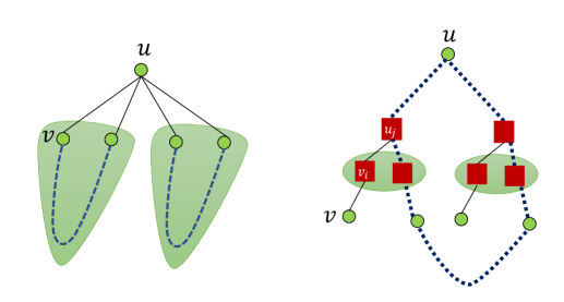
Figure 3: Left: Illustration of a node $u$ with two connected components in the original graph $G$. Right: The auxiliary graph $G^{\prime}$ and a new cycle found by the cycle cover in $G^{\prime}$ (dashed line). One can observe how this new cycle now connects the two connected components.

Now, we run the cycle cover algorithm on $G^{\prime}$. In the analysis section we show that since the graph $G$ is $2$-vertex connected, the graph $G^{\prime}$ is also $2$-vertex connected. A cycle covering an edge $(u,u_{j})$ in $G^{\prime}$ must use the virtual edge $(u,u_{i})$ for $i\neq j$. That is, this cycle is used to obtain a path between the ${j}\textsuperscript{th}$ connected component and the ${i}\textsuperscript{th}$ connected component of $u$ while avoiding $u$. Adding these paths will again reduce the number of connected components by a half. Finally, since these paths are computed in a virtual graph $G^{\prime}$, we need to translate them into $G$-paths. This is done as follows. An edge $(u,u_{j})$ is simply replaced by $u$. An edge $(u_{j},v_{i})$ is replaced by the edge $(u,v)$ in $G$. We then use the fact that the cycles computed in $G^{\prime}$ have low congestion in $G^{\prime}$, to show that also the translated paths have low congestion in $G$.

To bound the depth of the private tree $T(u)$, we note that the final tree has at most $\Delta$ neighbors of $u$. Each tree path connecting two consecutive $u$’s neighbors is obtained from a cycle cover computation and thus have length $O(D\log n)$. Overall, this gives a diameter of $O(\Delta D\log n)$. The detailed description and analysis of this construction are provided in Section 4.

3 Preliminaries

Unless stated otherwise, the logarithms in this paper are base 2. For an integer $n\in\mathbb{N}$ we denote by $[n]$ the set $\{1,\ldots,n\}$. We denote by $U_{n}$ the uniform distribution over $n$-bit strings. For two distributions (or random variables) $X,Y$ we write $X\equiv Y$ if they are identical distributions. That is, for any $x$ it holds that $\Pr[X=x]=\Pr[Y=x]$.

Graph Notations.

For a tree $T\subseteq G$, let $T(z)$ be the subtree of $T$ rooted at $z$. Let $\Gamma(u,G)$ be the neighbors of $u$ in $G$, and $\deg(u,G)=|\Gamma(u,G)|$. When $G$ is clear from the context, we simply write $\Gamma(u)$ and $\deg(u)$.

3.1 Distributed Algorithms

The Communication Model.

We use a standard message passing model, the ${\mathsf{CONGEST}}$ model [Pel00], where the execution proceeds in synchronous rounds and in each round, each node can send a message of size $O(\log n)$ to each of its neighbors. In this model, local computation at each node is for free and the primary complexity measure is the number of communication rounds. Each node holds a processor with a unique and arbitrary ID of $O(\log n)$ bits. Throughout, we make extensive use of the following useful tool, which is based on the random delay approach of [LMR94].

Theorem 4 ([Gha15, Theorem 1.3]).

Let $G$ be a graph and let $A_{1},\ldots,A_{m}$ be $m$ distributed algorithms in the ${\mathsf{CONGEST}}$model, where each algorithm takes at most d rounds, and where for each edge of $G$, at most c messages need to go through it, in total over all these algorithms. Then, there is a randomized distributed algorithm (using only private randomness) that, with high probability, produces a schedule that runs all the algorithms in $O(\mbox{\tt c}+\mbox{\tt d}\cdot\log n)$ rounds, after $O(\mbox{\tt d}\log^{2}n)$ rounds of pre-computation.

A Distributed Algorithm.

Consider an $n$-vertex graph $G$ with maximal degree $\Delta$. We model a distributed algorithm $A$ that works in $r$ rounds as describing $r$ functions $f_{1},\ldots,f_{r}$ as follows. Let $u$ be a node in the graph with input $x_{u}$ and neighbors $v_{1},\ldots,v_{\Delta}$. At any round $i$, the memory of a node $u$ consists of a state, denoted by $\sigma_{i}$ and $\Delta$ messages $m_{v_{1}\to u}\ldots,m_{v_{\Delta}\to u}$ that were received in the previous round.

Initially, we set $\sigma_{0}$ to contain only the input $x_{u}$ of $u$ and its ID and initialize all messages to $\bot$. At round $i$ the node $u$ updates its state to $\sigma_{i+1}$ according to its previous state $\sigma_{i}$ and the message from the previous round, and prepares $\Delta$ messages to send $m_{u\to v_{1}},\ldots,m_{u\to v_{\Delta}}$. To ease notation (and without loss of generality) we assume that each state contains the ID of the node $u$, thus, we can focus on a single update function $f_{i}$ for every round that works for all nodes. The function $f_{i}$ gets the state $\sigma_{i}$ and messages $m_{v_{1}\to u}\ldots,m_{v_{\Delta}\to u}$, and randomness $s_{i}$ and outputs the next state and outgoing message:

$$(\sigma_{i},m_{u\to v_{1}},\ldots,m_{u\to v_{\Delta}})\leftarrow f_{i}(\sigma_{i-1},m_{v_{1}\to u},\ldots,m_{v_{\Delta}\to u},s_{i}).$$

At the end of the $r$ rounds, each node $u$ has a state $\sigma_{r}$ and a final output of the algorithm. Without loss of generality, we assume that $\sigma_{r}$ is the final output of the algorithm (we can always modify $f_{r}$ accordingly).

Natural Distributed Algorithms.

We define a family of distributed algorithms which we call natural, which captures almost all known distributed algorithms. A natural distributed algorithm has two restrictions for any round $i$: (1) the size the state is bounded by $|\sigma_{i}|\leq\Delta\cdot\mathsf{polylog}(n)$, and (2) the function $f_{i}$ is computable in polynomial time. The input for $f_{i}$ is the state $\sigma_{i}$ and at most $\Delta$ message each of length $\log n$. Thus, the input length $m$ for $f_{i}$ is bounded by $m\leq\Delta\cdot\mathsf{polylog}(n)$, and the running time should be polynomial in this input length.

We introduce this family of algorithms mainly for simplifying the presentation of our main result. For these algorithms, our main statement can be described with minimal overhead. However, our results are general and work for any algorithm, with appropriate dependency on the size of the state and the running time the function $f_{i}$ (i.e., the internal computation time at each node $u$ in round $i$).

Notations.

We introduce some notations: For an algorithm ${\mathcal{A}}$, graph $G$, input $X=\{x_{v}\}_{v\in G}$ we denote by ${\mathcal{A}}_{u}(G,X)$ the random variable of the output of node $u$ while performing algorithm ${\mathcal{A}}$ on the graph $G$ with inputs $X$ (recall that ${\mathcal{A}}$ might be randomized and thus the output is a random variable and not a value). Denote by ${\mathcal{A}}(G,X)=\{{\mathcal{A}}_{u}(G,X)\}_{u\in G}$ the collection of outputs (in some canonical ordering). Let $\mathsf{View}_{u}^{{\mathcal{A}}}(G,X)$ be a random variable of the viewpoint of $u$ in the running of the algorithm ${\mathcal{A}}$. This includes messages sent to $u$, its memory and random coins during all rounds of the algorithm.

Secure Distributed Computation.

Let ${\mathcal{A}}$ be a distributed algorithm. Informally, we say that ${\mathcal{A}}^{\prime}$ simulates ${\mathcal{A}}$ in a secure manner if when running the algorithm ${\mathcal{A}}^{\prime}$ every node $u$ only learns its final output in ${\mathcal{A}}$ and “nothing more”. This notion is captured by the existence of a simulator and is defined below.

Definition 1 (Perfect Privacy).

Let ${\mathcal{A}}$ be a distributed (possibly randomized) algorithm, that works in $r$ rounds. We say that an algorithm ${\mathcal{A}}^{\prime}$ simulates ${\mathcal{A}}$ with perfect privacy if for every graph $G$, every $u\in G$ and it holds that:

1. Correctness: For every input $X=\{x_{v}\}_{v\in V}$: ${\mathcal{A}}(G,X)\equiv{\mathcal{A}}^{\prime}(G,X)$.

2. Perfect Privacy: There exists a randomized algorithm (simulator) $\mathsf{Sim}$ such that for every input $X=\{x_{v}\}_{v\in V}$ it holds that

   $$\mathsf{View}_{u}^{{\mathcal{A}}^{\prime}}(G,X)\equiv\mathsf{Sim}(G,x_{u},{\mathcal{A}}_{u}(G,X)).$$

This security definition is known as the “semi-honest” model, where the adversary, acting as one of the nodes in the graph, is not allowed to deviate from the prescribed protocol but can run arbitrary computation given all the messages it received. Moreover, we assume that the adversary does no collude with other nodes in the graph.

3.2 Cryptography with Perfect Privacy

One of the main cryptographic tools we use is a specific protocol for secure multiparty computation that has perfect privacy. Feige Kilian and Naor [FKN94] suggested a model where two players having inputs $x$ and $y$ wish to compute a function $f(x,y)$ in a secure manner. They achieve this by each sending a single message to a third party that is able to compute the output of the function $f$ from these messages but learn nothing else about the inputs $x$ and $y$. For the protocol to work, the two parties need to share private randomness that is not known to the third party. This model was later generalized to multi-players and is called the Private Simultaneous Messages Model [IK97], which we formally describe next.

Definition 2 (The $\mathsf{PSM}$ model).

Let $f\colon(\{0,1\}^{m})^{k}\to\{0,1\}^{m}$ be a $k$ variant function. A $\mathsf{PSM}$ protocol for $f$ consists of a pair of algorithms $(\mathsf{PSM.Enc},\mathsf{PSM.Dec})$ where $\mathsf{PSM.Enc}\colon\{0,1\}^{m}\times\{0,1\}^{r}\to\{0,1\}^{t}$ and $\mathsf{PSM.Dec}\colon(\{0,1\}^{t})^{k}\to\{0,1\}^{m}$ such that

• For any $X=(x_{1},\ldots,x_{k})$ it holds that: $\Pr_{R\in\{0,1\}^{r}}[\mathsf{PSM.Dec}(\mathsf{PSM.Enc}(x_{1},R),\ldots,\allowbreak\mathsf{PSM.Enc}(x_{k},R))\allowbreak=f(x_{1},\ldots,x_{k})]=1.$

• There exists a randomized algorithm (simulator) $\mathsf{Sim}$ such that for $X=x_{1},\ldots,x_{k}$ and for $R$ sampled from $\{0,1\}^{r}$, it holds that

  $$\left\{\mathsf{PSM.Enc}(x_{i},R)\right\}_{i\in[k]}\equiv\mathsf{Sim}(f(x_{1},\ldots,x_{k})).$$

The communication complexity of the PSM protocol is the encoding length $t$ and the randomness complexity of the protocol is defined to be $|R|=r$.

Theorem 5 (Follows from [IK97]).

For every function $f:(\{0,1\}^{m})^{k}\to\{0,1\}^{\ell}$ that is computable by an $s=s(m,k)$-space TM there is an efficient perfectly secure $\mathsf{PSM}$ protocol whose communication complexity and randomness complexity are $O(km\ell\cdot 2^{2s})$.

We describe two additional tools that we will use, secret sharing and one-time-pad encryption.

Definition 3 (Secret Sharing).

Let $x\in\{0,1\}^{n}$ be a message. We say $x$ is secret shared to $k$ shares by choosing $k$ random strings $x^{1},\ldots,x^{k}\in\{0,1\}^{n}$ conditioned on $x=\bigoplus_{j=1}^{k}x^{j}$. Each $x^{j}$ is called a share, and notice that the joint distribution of any $k-1$ shares is uniform over $(\{0,1\}^{n})^{k-1}$.

Definition 4 (One-Time-Pad Encryption).

Let $x\in\{0,1\}^{n}$ be a message. A one-time pad is an extremely simple encryption scheme that has information theoretic security. For a random key $K\in\{0,1\}^{n}$ the “encryption” of $x$ according to $K$ is $\widehat{x}=x\oplus K$. It is easy to see that the encrypted message $\widehat{x}$ (without the key) is distributed as a uniform random string. To decrypt $\widehat{x}$ using the key $K$ we simply compute $x=\widehat{x}\oplus K$. The key $K$ might be referenced as the encryption key or decryption key.

4 Private Neighborhood Trees

The graph theoretic basis for our compiler is given by Private Neighborhood Trees, a decomposition of the graph $G$ into (possibly overlapping) trees $T(u_{1}),\ldots,T(u_{n})$ such that each tree $T(u_{i})$ contains the neighbors of $u_{i}$ in $G$ but does not contain $u_{i}$. Each tree $T(u_{i})$ provides the neighbors of $u_{i}$ a way to communicate privately without their root $u_{i}$. The goal is to compute a collection of trees with small overlap and small diameter. Thus, we are interested in the existence of a low-congestion private neighborhood trees.

Definition 5 (Private Neighborhood Trees).

Let $G=(V=\{u_{1},\ldots,u_{n}\},E)$ be a $2$-vertex connected graph. The private neighborhood trees ${\cal N}$ of $G$ is a collection of $n$ subtrees $T(u_{1}),\ldots,T(u_{n})$ in $G$ such that for every $i\in\{1,\ldots,n\}$ it holds that $\Gamma(u_{i})\setminus\{u_{i}\}\subseteq T(u_{i})$, but $u_{i}\notin T(u_{i})$. A $(\mbox{\tt d},\mbox{\tt c})$-private neighborhood trees ${\cal N}$ satisfies:

1. $\mathsf{Diam}(T(u_{i}))\leq\mbox{\tt d}$ for every $i\in\{1,\ldots,n\}$,

2. Every edge $e\in E$ appears in at most c trees.

Note that since the graph is $2$-vertex connected, all the neighbors of $u$ are indeed connected in $G\setminus\{u\}$ for every node $u$. The main challenge is in showing that all $n$ trees can be both of small diameter and with small overlap.

Theorem 2 (Private Trees).

For every $2$-vertex connected graph $G$ with maximum degree $\Delta$ and diameter $D$, there exists a $(\mbox{\tt d},\mbox{\tt c})$-private trees with $\mbox{\tt d}=O(D\cdot\Delta\cdot\log n)$ and $\mbox{\tt c}=O(D\cdot\log\Delta\cdot\log^{3}n)$.

Proof.

The construction of the private neighborhood trees ${\cal N}$ consists of $\ell=\log\Delta$ phases. In each phase, we compute an $(O(D\log n),O(\log^{3}n))$ cycle cover in some auxiliary graph using the cycle cover algorithm in [PY18]. We begin by having each node $u$ holding an empty forest $F_{0}(u)=(\Gamma(u,G),\emptyset)$ consisting only of $u$’s neighbors. Then, in each phase we add edges to these forests such that the number of connected components (containing the neighbors $\Gamma(u,G)$) is reduced by a factor of $2$. After $\ell$ phases, we have a single connected component, that is, we have that every $u\in V$ has a tree $T(u)$ in $G\setminus\{u\}$ that spans all neighbors $\Gamma(u,G)$. Let ${\cal C}_{0}$ be a cycle cover of $G$. For every phase $t\in\{0,\ldots,\ell\}$, let $CC_{t}(u)$ be the number of connected components in the forest $F_{t}(u)$. Note that $CC_{0}(u)=\deg(u)$ for all nodes $u$.

In each phase $t\geq 1$, we have a collection of forests $\mathcal{N}_{t-1}=\{F_{t-1}(u_{1}),\ldots,F_{t-1}(u_{n})\}$ that satisfy the following for every $u_{i}$:

1. $F_{t-1}(u_{i})\subseteq G\setminus\{u_{i}\}$ (the forest avoids $u_{i}$).

2. $\Gamma(u_{i})\subseteq V(F_{t-1}(u_{i}))$ (the forest contains all neighbors of $u_{i}$).

3. $F_{t-1}(u_{i})$ has $CC_{t-1}(u_{i})\leq\deg(u_{i})/2^{t-1}$ connected components.

It is easy to see that these conditions are met for phase $t=0$, when we have the empty forest that simply contains all the neighbors of $u_{i}$. The goal of phase $t$ is to add edges to each $F_{t-1}(u_{i})$ in order to reduce the number of connected components by factor $2$. The algorithm uses the current collection of forests $\mathcal{N}_{t-1}$ to define an auxiliary graph $\widetilde{G}_{t}$ which contains the nodes of $G$ and some additional “virtual” nodes and a different set of edges.

For every $u\in V$, we add to $\widetilde{G}_{t}$ a set of $k=CC_{t-1}(u)$ virtual nodes $\widetilde{u}_{1},\ldots,\widetilde{u}_{k}$, one for each connected component. We connect $u$ to each of its virtual copies $\widetilde{u}_{i}$ by adding the edges $(u,\widetilde{u}_{i})$. Let $(u,v)\in E$ be an edge such that $v$ is in the ${j}\textsuperscript{th}$ connected component of $u$, and $u$ is in the ${i}\textsuperscript{th}$ connected component of $v$. Then we add the edge $(\widetilde{u_{j}},\widetilde{v_{i}})$ to the graph $\widetilde{G}_{t}$. The graph $\widetilde{G}_{t}$ has $O(m)$ nodes, $O(m)$ edges and diameter at most $3D$. To see this, any edge $(u,v)$ in the original graph $G$ can be replaced with the path $u\to\widetilde{u}_{j}\to\widetilde{v}_{i}\to v$.

Next, we compute an $(O(D\log n),O(\log^{3}n))$-cycle cover $\widetilde{{\cal C}}_{t}$ for the edges of $\widetilde{G}_{t}$. In the analysis part (Cl. 1), we show that $\widetilde{G}_{t}$ is also $2$-vertex connected, and hence all its edges are covered by cycles of $\widetilde{{\cal C}}_{t}$. To map these virtual cycles to real cycles ${\cal C}_{t}$ in $G$, we simply replace a virtual node $\widetilde{u}_{j}$ with the real node $u$. An edge $(u,\widetilde{u}_{j})$ will be contracted to just $u$, and edge $(\widetilde{u}_{j},\widetilde{v}_{i})$ will be replaced by $(u,v)$.

Let $G_{t}(u)$ be the forest $F_{t-1}(u)$ obtained by adding to it all the edges of the cycles in ${\cal C}_{t}$ that intersect $u$, but avoiding the node $u$. That is, we define

$$G_{t}(u)=F_{t-1}(u)\cup\{C\in{\cal C}_{t}~{}\mid~{}u\in C\}\setminus\{u\}.$$

Moreover, let $F_{t}(u)\subseteq G_{t}(u)$ be a forest that spans all the neighbors of $u$. This forest can be computed, for instance, by running a BFS from a neighbor of $u$ in each connected component of $G_{t}(u)$. This completes the description of phase $t$. The final private tree collection is given by ${\cal N}=\{F_{\ell}(u_{1}),\ldots,F_{\ell}(u_{n})\}$. We now turn to analyze this construction and prove Theorem 2.

Correctness.

We start by proving each $F_{\ell}(u_{i})$ is a tree. Note that we run the cycle cover algorithm on the graph $\widetilde{G}_{t}$. To obtain a cycle for each edge in $\widetilde{G}_{t}$ it is required to show that $\widetilde{G}_{t}$ is 2-edge connected. We show the stronger property that it is in fact a 2-vertex connected.

Claim 1.

For every phase $t\in[\ell]$, the graph $\widetilde{G}_{t}$ is 2-vertex connected.

Proof.

Recall that the graph $G$ is 2-vertex connected, and that any edge $(u,v)$ in the original graph $G$ can be replaced with the path $u\to\widetilde{u}_{j}\to\widetilde{v}_{i}\to v$ in $\widetilde{G}_{t}$.

Let $u\in G$ be a (real) node and consider removing a node $u^{\prime}\in\{u,\widetilde{u}_{1},\ldots,\widetilde{u}_{k}\}$ from $\widetilde{G}_{t}$. We will show that the graph $\widetilde{G}_{t}\setminus\{u^{\prime}\}$ remains connected. Let $w_{1},w_{2}$ be two nodes in $\widetilde{G}_{t}\setminus\{u^{\prime}\}$. Let $w^{\prime}_{1}$ be the closest node to $w_{1}$ in $\widetilde{G}_{t}\setminus\{u^{\prime}\}$ such that $w^{\prime}_{1}\in G\setminus{u}$ (it might be that $w_{1}=w^{\prime}_{1}$). We observe that such a node $w^{\prime}_{1}$ always exists: if $w_{1}\in G\setminus\{u\}$ then $w^{\prime}_{1}=w_{1}$, if $w_{1}=\widetilde{v}_{i}$ for some $i$ and $v\neq u$ then $w^{\prime}_{1}=v$ and if $w_{1}=\widetilde{u}_{i}$ for some $i$ then there exists $v\neq u$ such that $(v,u)\in G$ and therefore there exists $i^{\prime}$ such that $\widetilde{v}_{i^{\prime}}$ is connected to $\widetilde{u}_{i}$ and then $w^{\prime}_{1}=v$. Similarly, let $w^{\prime}_{2}$ be the closest node to $w_{2}$ in $\widetilde{G}_{t}\setminus\{u^{\prime}\}$ such that $w^{\prime}_{2}\in G\setminus\{u\}$ (it might be that $w^{\prime}_{1}=w^{\prime}_{2}$).

Since $G$ is 2-vertex connected, then there is a path $P$ in $G$ between $w^{\prime}_{1}$ and $w^{\prime}_{2}$ that does not use $u$. Therefore, there is a path $\widetilde{P}$ between $w^{\prime}_{1}$ and $w^{\prime}_{2}$ in $\widetilde{G}_{t}$ that does not use $u$ or $\widetilde{u}_{j}$ for any $j\in[k]$. Thus, there is a path in $\widetilde{G}_{t}$ from $w_{1}$ to $w_{2}$ as follows: $w_{1},\ldots,w^{\prime}_{1},\widetilde{P},w^{\prime}_{2},\ldots,w_{2}$. Note that it might be the case that this path is not simple (e.g., if $\widetilde{P}$ uses $w_{1}$) but it can be made simple by omitting internal cycles. ∎

Next, we show that indeed the final forests are trees.

Claim 2.

For every phase $t\in[\ell]$ and for every $u\in V$ the number of connected components satisfies $CC_{t}(u)\leq\Delta/2^{t}$.

Proof.

The lemma is shown by induction on $t$. The case of $t=0$ holds vacuously. Assume that the claim holds up to $t-1$ and consider phase $t$. By construction, for each $u$, the auxiliary graph $\widetilde{G}_{t}$ contains $CC_{t-1}(u)$ virtual nodes $\widetilde{u}_{j}$ that are connected to $u$.

The cycle cover $\widetilde{{\cal C}}_{t}$ for $\widetilde{G}_{t}$ covers all these virtual edges $(u,\widetilde{u}_{j})$ by virtual cycles, each such cycle connects two virtual nodes. Since every two virtual nodes of $u$ in $\widetilde{G}_{t}$ are connected to neighbors of $u$ that belong to different components in $G_{t-1}(u)$, every cycle that connects two virtual neighbors is mapped into a cycle that connects two of $u$’s neighbors that belong to a different connected component in phase $G_{t-1}(u)$. Hence, the number of connected components in the forest $F_{t}(u)$ has been decreased by factor at least $2$ compared to that of $F_{t-1}(u)$. ∎

Small Diameter.

We show that the diameter of each tree $T(u_{i})$ is bounded by $O(\Delta D\cdot\log n)$. Note that this bound is existentially tight (up to logarithmic factors) as there are graphs $G$ with diameter $D$ and a node $u$ with degree $\Delta$ such that the diameter of $G\setminus\{u\}$ is $O(\Delta D)$.

Claim 3.

The diameter of each tree $T(u_{i})\in{\cal N}$ is $O(\Delta\cdot D\cdot\log n)$.

Proof.

Note that the forest $F_{t}(u)$ is formed by a collection of $O(D\log n)$-length cycles that connect $u$’s neighbors. Hence, when removing $u$, we get paths of length $O(D\log n)$. Consider the process where in each phase $t$, every two $u$’s-neighbors that are connected by a cycle in ${\cal C}_{t}$ are connected by a single “edge”. By the Proof of Claim 2, after $\log\Delta$ phases, we get a connected tree with $\deg(u)$ nodes, and hence of “diameter” $\deg(u)$. Since each edge corresponds to a path of length $O(D\log n)$ in $G$, we get that the final diameter of $F_{\ell}(u)$ is $O(\deg(u)\cdot D\cdot\log n)$. ∎

Congestion.

We analyze the congestion of the construction.

Claim 4.

Each edge $e$ appears on at most $O(D\log^{3}n\log\Delta)$ different trees $T(u_{i})\in{\cal N}$.

Proof.

We first show that the cycles ${\cal C}_{t}$ computed in $G$ have congestion $O(\log^{3}n)$ for every $t\in\{1,\ldots,\ell\}$. Clearly, the cycles $\widetilde{{\cal C}}_{t}$ computed in $\widetilde{G}_{t}$ have congestion of $O(\log^{3}n)$. Consider the mapping of cycles $\widetilde{{\cal C}}_{t}$ in $\widetilde{G}_{t}$ to a cycles ${\cal C}_{t}$ in $G$. Edges of the type $(u,\widetilde{u}_{j})$ are replaced by $(u,u)$ and hence there is no real edge in the cycle. Edges of the type $(\widetilde{u}_{j},\widetilde{v}_{i})$ are replaced by $(u,v)$. Since there is only one virtual node of $u$ that connects to $v$, and since $(\widetilde{u}_{j},\widetilde{v}_{i})$ appears in $O(\log^{3}n)$ many cycles, also $(u,v)$ appears in $O(\log^{3}n)$ many cycles (i.e., this conversion does not increase the congestion).

Note that the cycle $C$ of each edge $(u,v)$ joins the $G_{t}$ subgraphs of at most $D$ nodes since in our construction a cycle $C$ might cover up to $D$ edges. In addition, each edge $e^{\prime}$ appears on different cycles in ${\cal C}_{t}$.

We now claim that each edge $e$ appears on $O(t\log^{3}n\cdot D)$ graphs $G_{t}(u)$. For $t=1$, this holds as the cycle $C$ of an edge $(u,v)$ joins the subgraphs $G_{1}(x)$ and $G_{1}(y)$ for every edge $(x,y)$ that is covered by $C$. Assume it holds up to $t-1$ and consider phase $t$. In phase $t$, we add to the $G_{t}(u)$ graphs the edges of ${\cal C}_{t}$. Again, each cycle $C^{\prime}$ of an edge $(u,v)$ joins $D$ graphs $G_{t}(x),G_{t}(y)$ for every $(x,y)$ that is covered by $C^{\prime}$. Hence each edge $e$ appears on $O(D\cdot\log^{3}n)$ of the subgraphs $G_{t}(u_{j})\setminus G_{t-1}(u_{j})$. By induction assumption, each $e$ appears on $(t-1)\log^{3}n\cdot D$ graphs $G_{t-1}(u_{j})$ and hence overall each edge $e$ appears on $O(t\log^{3}n)$ graphs $G_{t}(u_{j})$. Therefore we get that each edge appears on $O(\log\Delta\cdot\log^{3}n\cdot D)$ trees in ${\cal N}$. ∎

The above proof actually shows a slightly stronger statement: a construction of $(\mbox{\tt d},\mbox{\tt c})$-cycle covers yields a $(\mbox{\tt d}^{\prime},\mbox{\tt c}^{\prime})$ private neighborhood trees for $\mbox{\tt d}^{\prime}=O(\mbox{\tt d}\cdot\Delta)$ and $\mbox{\tt c}^{\prime}=O(\mbox{\tt c}\cdot\mbox{\tt d}\cdot\log\Delta)$. ∎ The distributed construction of private neighborhood trees is in Appendix A.

5 Secure Simulation via Private Neighborhood Trees

In this section, we describe how to transform any distributed algorithm ${\cal A}$ to a new algorithm ${\cal A}^{\prime}$ which has the same functionality as ${\cal A}$ (i.e., the output for every node $u$ in ${\cal A}$ is the same as in ${\cal A}^{\prime}$) but has perfect privacy (as is defined in Definition 1). Towards this end, we assume that the combinatorial structures required are already computed (in a preprocessing stage described in Appendix A), namely, a private neighborhood tree in the graph. The output of the preprocessing stage is given in a distributed manner. The (distributed) output of the private neighborhood trees for each node $u$, is such that each vertex $v$ knows its parent in the private neighborhood tree of $u$ (if such exists).

Theorem 1.

Let $G$ be an $n$-vertex graph with diameter $D$ and maximal degree $\Delta$. Let ${\mathcal{A}}$ be a natural distributed algorithm that works on $G$ in $r$ rounds. Then, ${\mathcal{A}}$ can be transformed to a new algorithm ${\mathcal{A}}^{\prime}$ with the same output distribution and which has perfect privacy and runs in $\widetilde{O}(rD\cdot\mathsf{poly}(\Delta))$ rounds (after a preprocessing stage).

As a preparation for our secure simulation, we provide the following convenient view of distributed algorithms.

5.1 Our Framework

We treat the distributed $r$-round algorithm ${\cal A}$ from the viewpoint of some fixed node $u$, as a collection of $r$ functions $f_{1},\ldots,f_{r}$ as follows. Let $\Gamma(u)=\{v_{1},\ldots,v_{k}\}$. At any round $i$, the memory of $u$ consists of a state, denoted by $\sigma_{i}$ and $\Delta$ messages $m_{v_{1}\to u}\ldots,m_{v_{\Delta}\to u}$ that were received in the previous round (in the degree of the node is less than $\Delta$ the rest of the messages are empty). Initially, we set $\sigma_{0}$ to be a fixed string and initialize all messages to NULL. At round $i$ the node $u$ updates its state to $\sigma_{i+1}$ according to its previous state $\sigma_{i}$ and the messages that it got in the previous round. It then prepares $k$ messages to send $m_{u\to v_{1}},\ldots,m_{u\to v_{\Delta}}$. To ease notation (and without loss of generality), we assume that each state contains the ID of the node $u$. Thus, we can focus on a single update function $f_{i}$ for every round that works for all nodes. The function $f_{i}$ gets the state $\sigma_{i}$, the messages $m_{v_{1}\to u}\ldots,m_{v_{\Delta}\to u}$, and the randomness $s$. The output of $f_{i}$ is the next state $\sigma_{i+1}$, and at most $k$ outgoing messages:

$$(\sigma_{i},m_{u\to v_{1}},\ldots,m_{u\to v_{\Delta}})\leftarrow f_{i}(\sigma_{i-1},m_{v_{1}\to u},\ldots,m_{v_{\Delta}\to u},s).$$

Our compiler works round-by-round where each round $i$ is replaced by a collection of rounds that “securely” compute $f_{i}$, in a manner that will be explained next. The complexity of our algorithm depends exponentially on the space complexity of the functions $f_{i}$. Thus, we proceed by transforming the original algorithm ${\cal A}$ to one in which each $f_{i}$ can be computed in logarithmic space, while slightly increasing the number of rounds.

Claim 5.

Any natural distributed algorithm ${\cal A}$ the runs in $r$ rounds can be transformed into a new algorithm $\widehat{{\cal A}}$ with the same output distribution such that $\widehat{{\mathcal{A}}}$ is computable in logarithmic space using $r^{\prime}=r\cdot\mathsf{poly}(\Delta+\log n)$ rounds.

Proof.

Let $t$ be the running time of the function $f_{i}$. Then, $f_{i}$ can be computed with a circuit of at most $t$ gates. Note that since ${\cal A}$ is natural, it holds that $t\leq\mathsf{poly}(\Delta,\log n)$.

Instead of letting $u$ computing $f_{i}$ in round $i$, we replace the $i$th round by $t$ rounds where each round computes only a single gate of the function $f_{i}$. These new rounds will have no communication at all, but are used merely for computing $f_{i}$ with a small amount of memory.

Let $g_{1},\ldots,g_{t}$ be the gates of the function $f_{i}$ in a computable order where $g_{t}$ is the output of the function. We define a new state $\sigma^{\prime}_{i}$ of the form $\sigma^{\prime}=(\sigma_{i},g_{1},\ldots,g_{t})$, where $\sigma_{i}$ is the original state, and $g_{j}$ is the value of the $j$th gate. Initially, $g_{1},\ldots,g_{t}$ are set to $\bot$. Then, for all $j\in[t]$ we define the function

$$f^{j}_{i}(\sigma_{i},g_{1},\ldots,g_{j-1},\bot,\ldots,\bot)=(\sigma_{i},g_{1},\ldots,g_{j-1},g_{j},\bot,\ldots,\bot).$$

In the $j$th round, we compute $f^{j}_{i}$, until the final $g_{t}$ is computed. Note that $f^{j}_{i}$ can be computed with logarithmic space, and since $t\leq\mathsf{poly}(\Delta,\log n)$ we can compute $f^{j}_{i}$ with space $O(\log\Delta+\log\log n)$. As a result, the $r$-round algorithm ${\cal A}$ is replaced by an $rt$-round algorithm $\widehat{{\cal A}}$, where $t\leq\mathsf{poly}(\Delta,\log n)$. That is, we have that $r^{\prime}\leq\mathsf{poly}(\Delta,\log n)$. ∎

As we will see, our compiler will have an overhead of $\mathsf{poly}(\Delta,\log n)$ in the round complexity and hence the overhead of Claim 5 is insignificant. Thus, we will assume that the distributed algorithm ${\cal A}$ satisfies that all its functions $f_{i}$ are computable in logarithmic space (i.e., we assume that the algorithm is already after the above transformation).

5.2 Secure Simulation of a Single Round

In the algorithm ${\cal A}$ each node $u$ computes the function $f_{i}$ in each round $i$. In our secure algorithm ${\cal A}^{\prime}$ we want to simulate this computation, however, on encrypted data, such that $u$ does not get to learn the true output of $f_{i}$ in any of the rounds except for the last one. When we say “encrypted” data, we mean a “one-time-pad” (see Definition 4). That is, we merely refer to a process where we the data is masked by XORing it with a random string $R$. Then, $R$ is called the encryption (and also decryption) key. Using this notion, we define a related function $f^{\prime}_{i}$ that, intuitively, simulates $f_{i}$ on encrypted data, by getting encrypted state and messages as input, decrypting them, then computing $f_{i}$ and finally encrypting the output with a new key. We simulate every round of the original algorithm ${\mathcal{A}}$ by a $\mathsf{PSM}$ protocol for the function $f^{\prime}_{i}$.

The Secure Function $f^{\prime}_{i}$.

The function $f^{\prime}_{i}$ gets the following inputs (encrypted elements will be denoted by the $\widehat{\cdot}$ notation):

1. An encrypted state $\widehat{\sigma}_{i-1}$ and encrypted messages $\{\widehat{m}_{v_{j}\to u}\}_{j=1}^{\Delta}$.

2. The decryption key $R_{\sigma_{i-1}}$ of the state $\widehat{\sigma}_{i-1}$ and the decryption keys $\{R_{v_{j}\to u}\}_{j}^{\Delta}$ for the messages $\{\widehat{m}_{v_{j}\to u}\}_{j=1}^{\Delta}$.

3. Shares for randomness $\{R^{j}_{s}\}_{j=1}^{\Delta}$ for the function $f_{i}$.

4. Encryption keys for encrypting the new state $R_{\sigma_{i}}$ and messages $\{R_{u\to v_{j}}\}_{j=1}^{\Delta}$.

The function $f^{\prime}_{i}$ decrypts the state and messages and runs the function $f_{i}$ (using randomness $s=\bigoplus R^{j}_{s}$) to get the new state $\sigma_{i}$ and the outgoing messages $m_{u\to v_{1}},\ldots,m_{u\to v_{\Delta}}$. Then, it encrypts the new state and messages using the encryption keys. In total, the function $f^{\prime}_{i}$ has $O(\Delta)$ input bits. The precise description of $f^{\prime}_{i}$ is given in Figure 4.

The description of the function $f^{\prime}_{i}$. Input: An encrypted state $\widehat{\sigma}_{i-1}$, encrypted messages $\left\{\widehat{m}_{v_{j}\to u}\right\}_{j=1}^{\Delta}$, keys for decrypting the input $R_{\sigma_{i-1}},\left\{R_{v_{j}\to u}\right\}_{j}^{\Delta}$, randomness $\left\{R^{j}_{s}\right\}_{j=1}^{\Delta}$ and keys for encrypting the output $R_{\sigma_{i}},\left\{R_{u\to v_{j}}\right\}_{j=1}^{\Delta}$. Run: 1. Compute $\sigma_{i-1}\leftarrow\widehat{\sigma}_{i-1}\oplus R_{\sigma_{i-1}}$ and $s\leftarrow\left(\bigoplus_{j=1}^{\Delta}R^{j}_{s}\right)$. 2. For $j=1\ldots\Delta$: compute $m_{v_{j}\to u}\leftarrow\widehat{m}_{v_{j}\to u}\oplus R_{v_{j}\to u}$. 3. Run $\sigma_{i},m_{u\to v_{1}},\ldots,m_{u\to v_{\Delta}}\leftarrow f(\sigma_{i-1},m_{v_{1}\to u},\ldots,m_{v_{\Delta}\to u},s)$. 4. Compute $\widehat{\sigma_{i}}\leftarrow\sigma_{i}\oplus R_{\sigma_{i}}$. 5. For $j=1\ldots\Delta$: compute $\widehat{m}_{u\to v_{j}}\leftarrow m_{u\to v_{j}}\oplus R_{u\to v_{j}}$. 6. Output $\widehat{\sigma_{i}},\widehat{m}_{u\to v_{1}},\ldots,\widehat{m}_{u\to v_{\Delta}}$.

Figure 4: The function $f^{\prime}_{i}$.

Recall that in the $\mathsf{PSM}$ model, we have $k$ parties $p_{1},\ldots,p_{k}$ and a server $s$, where it was assumed that all parties have private shared randomness (not known to $s$). Our goal is to compute $f^{\prime}_{i}$ securely by implementing a $\mathsf{PSM}$ protocol for all nodes in the graph simultaneously.

The compiler securely computes $f^{\prime}_{i}$ by simulating the $\mathsf{PSM}$ protocol for $f^{\prime}_{i}$, treating $u$ as the server and its immediate neighborhood as the parties. In order to exchange the private randomness, we use the notion of private neighborhood trees.

A private neighborhood tree collection consists of $n$ trees, a tree $T_{u}$ for every $u$, that spans all the neighbors of $u$ (i.e., the parties) without going through $u$, i.e., $T_{u}\subseteq G\setminus\{u\}$. Using this tree, all the parties can compute shared private random bits $R$ which are not known to $u$. For a single node $u$, this can be done in $O(\mathsf{Diam}(T_{u})+|R|)$ rounds, where $\mathsf{Diam}(T_{u})$ is the diameter of the tree and $R$ is the number of random bits. Clearly, our objective is to have trees $T_{u}$ with small diameter. Furthermore, as we wish to implement this kind of communication in all $n$ trees, $T_{u_{1}},\ldots,T_{u_{n}}$ simultaneously, a second objective is to have small overlap between the trees. That is, we would like each edge $e$ to appear only on a small number of trees $T_{u}$ (as on each of these trees, the edge is required to pass through different random bits). These two objectives are encapsulated in our notion of private-neighborhood-trees. The final algorithm ${\mathcal{A}}^{\prime}_{i}(u)$ for securely computing $f^{\prime}_{i}$ is described in Figure 5.

The algorithm ${\mathcal{A}}^{\prime}_{i}(u)$ for securely computing $f^{\prime}_{i}$. Input: Each node $v\in\Gamma(u)$ has input $x_{v}\in\{0,1\}^{m}$. 1. Let $T_{u}$ be the tree spanning $\Gamma(u)$ in $G\setminus\{u\}$ and let $w$ be the root. 2. $w$ chooses a random string $R$ and sends it to $\Gamma(u)$ using the tree $T_{u}$. 3. Each node $v\in\Gamma(u)$ computes $M_{v}=\mathsf{PSM.Enc}(f^{\prime}_{i},x_{v},R)$ and sends it to $u$. 4. $u$ computes $y=\mathsf{PSM.Dec}\left(f^{\prime}_{i},\{M_{v}\}_{v\in\Gamma(u)}\right)$.

Figure 5: The description of the distributed $\mathsf{PSM}$ algorithm of node $u$ for securely computing the function $f^{\prime}_{i}$.

In what follows analyze the security and round complexity of Algorithm ${\mathcal{A}}^{\prime}_{i}$.

Round Complexity.

Let $f:\{0,1\}^{m\cdot|\Gamma(u)|}\to\{0,1\}^{\ell}$ be a function with $|\Gamma(u)|\leq\Delta$ inputs, where each input is of length $m$ bits. The communication complexity of the $\mathsf{PSM}$ protocol depends on the input and output length of the function and also on the memory required to compute $f$. Suppose that $f$ is computable by an $s$-space Turing Machine (TM). Then, by Theorem 5 the communication complexity (and randomness complexity) of the protocol is at most $O(\Delta m\ell\cdot 2^{2s})$.

In the first phase of the protocol, the root $w$ sends a collection of random bits $R$ to $\Gamma(u)$ using the private neighborhood trees, where $|R|=O(\Delta\cdot m\cdot\ell\cdot 2^{2s})$. By Theorem 2, the diameter of the tree is at most $\widetilde{O}(D\Delta)$ and each edge belongs to $\widetilde{O}(D)$ different trees. Therefore, there are total of $\widetilde{O}(D\cdot|R|)$ many bits that need to go through a single edge when sending the information on all trees simultaneously. Using the random delay approach of Theorem 4, this can be done in $\widetilde{O}(D\Delta+D\cdot|R|)=\widetilde{O}(\Delta\cdot D\cdot m\cdot\ell\cdot 2^{2s})$ rounds. This is summarized by the following Lemma:

Lemma 1.

Let $f:(\{0,1\}^{m})^{\Delta}\to\{0,1\}^{\ell}$ be a function over $\Delta$ inputs where each is of length at most $m$ and that is computable by a $s$-space Turing Machine. Then, there is a distributed algorithm ${\mathcal{A}}^{\prime}_{i}(u)$ (in the $\mathsf{CONGEST}$ model) with perfect privacy where each node $u$ outputs $f$ evaluated on $\Gamma(u)$. The round complexity of ${\mathcal{A}}^{\prime}_{i}(u)$ is $\widetilde{O}(\Delta\cdot D\cdot m\cdot\ell\cdot 2^{2s})$.

5.3 The Final Secure Algorithm

Using the function $f^{\prime}_{i}$, we define the algorithm ${\cal A}^{\prime}_{u}$ for computing the next state and messages of the node $u$. We describe the algorithm for any $u$ in the graph, and at the end, we show that all the algorithms $\{{\cal A}^{\prime}_{u}\}_{u\in G}$ can be run simultaneously with low congestion.

The algorithm ${\cal A}^{\prime}_{u}$ involves running the distributed algorithm ${\mathcal{A}}^{\prime}_{i}(u)$ for each round $i\in\{1,\ldots,r\}$. The secure simulation of round $i$ starts by letting the root of each tree $T_{u}$ (i.e., the tree connecting the neighbors of $u$ in $G\setminus\{u\}$) sample a key $R_{\sigma_{i}}$ for encrypting the new state of $u$. Moreover, each neighbor $v_{j}$ of $u$ samples a share of the randomness $R^{j}_{s}$ used to evaluate the function $f_{i}$, and a key $R_{u\to v_{j}}$ for encrypting the message sent from $u$ to $v_{j}$.

Then they run ${\mathcal{A}}^{\prime}_{i}(u)$ algorithm with $u$ as the server and $\Gamma(u)$ as the parties for computing the function $f^{\prime}_{i}$ (see Figure 5). The node $u$ has the encrypted state and message, the neighbors of $u$ have the (encryption and decryption) keys for the current state, the next state and the sent messages, and moreover the randomness for evaluating $f^{\prime}_{i}$. At the end of the protocol, $u$ computes the output of $f^{\prime}_{i}$ which is the encrypted output of the function $f_{i}$.

After the final round, $u$ holds an encryption of the final state $\widehat{\sigma_{r}}$ which contains only the output of the original algorithm ${\mathcal{A}}$. At this point, the neighbors of $u$ send it the decryption key for this last state, $u$ decrypts its state and outputs the decrypted state. Initially, the state $\sigma_{0}$ is a fixed string which is not encrypted, and the encryption keys for this round are assumed to be $0$. The description is summarized in Figure 6. See Figure 7 for an illustration.

The description of the algorithm ${\cal A}^{\prime}_{u}$. 1. Let $v_{1},v_{2},\ldots,v_{\Delta}$ be some arbitrary ordering on $\Gamma(u)$. 2. For each round $i=1\ldots r$ do: (a) $u$ sends $\widehat{\sigma}_{i-1}$ to neighbor $v_{2}$. (b) Each neighbor $v_{j}$ of $u$ samples $R^{j}_{s}$ at random (and stores it). (c) $v_{1}$ chooses $R_{\sigma_{i}}$ at random (and stores it). (d) Run the ${\mathcal{A}}_{i}(u)$ algorithm for $f^{\prime}_{i}$ with server $u$ and parties $\Gamma(u)$ where: i. $v_{1}$ has an inputs $R_{\sigma_{i-1}}$ and $R_{\sigma_{i}}$ and $v_{2}$ has input $\widehat{\sigma}_{i-1}$. ii. In addition, each neighbor $v_{j}$ of $u$ has input $R_{u\to v_{j}},R^{j}_{s}$. iii. $u$ learns the final output of the algorithm $(\widehat{\sigma_{i}},\widehat{m}_{u\to v_{1}},\ldots,\widehat{m}_{u\to v_{\Delta}})$. 3. $v_{1}$ sends $R_{\sigma_{r}}$ to $u$. 4. $u$ computes $\sigma_{r}=\widehat{\sigma}_{r}\oplus R_{\sigma_{r}}$ and outputs $\sigma_{r}$.

Figure 6: The description of the Algorithm ${\cal A}^{\prime}_{u}$. We assume that in “round 0” all keys are initialized to 0. That is, we let $R_{\sigma_{0}}=0$, and initially set $R_{v_{j}\to u}=0$ for all $j\in[\Delta]$.

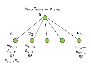
Figure 7: The information held by $u$ and its neighbors in phase $i$ of the algorithm.

Finally, we show that the protocol is correct and secure.

Correctness.

The correctness follows directly from the construction. Consider a node $u$ in the graph. Originally, $u$ computes the sequence of states $\sigma_{0},\ldots,\sigma_{r}$ where $\sigma_{r}$ contained the final output of the algorithm. In the compiled algorithm ${\mathcal{A}}^{\prime}$, for each round $i$ of ${\cal A}$ and every node $u$ the sub-algorithm ${\mathcal{A}}^{\prime}_{i}(u)$ computes $\widehat{\sigma_{i}}$, where $\widehat{\sigma_{i}}=\sigma_{i}\oplus R_{\sigma_{i}}$ where $v_{1}$ holds $R_{\sigma_{i}}$. Thus, after the last round, $u$ has $\widehat{\sigma_{r}}$ and $v_{1}$ has $R_{\sigma_{r}}$. Finally, $u$ computes $\widehat{\sigma}_{r}\oplus R_{\sigma_{r}}=\sigma_{r}$ and outputs $\sigma_{r}$ as required.

Round Complexity.

We compute the number of rounds of the algorithm for any natural algorithm ${\mathcal{A}}$. The algorithm consists of $r^{\prime}=r\cdot\mathsf{poly}(\Delta+\log n)$ iterations. In each iteration, every vertex $u$ implements algorithm ${\mathcal{A}}^{\prime}_{i}$ for the function $f^{\prime}_{i}$ (there are other operations in the iteration but they are negligible). We know that $f_{i}$ can be computed in $s$-space where $s=O(\log\Delta+\log\log n)$, and thus we can bound the size of each input to $f^{\prime}_{i}$ by $\mathsf{poly}(\Delta)\cdot\mathsf{polylog}(n)$. Indeed, the state has this bound by the definition of a natural algorithm, and thus also the encrypted state (which has the exact same size), the messages and encryption keys for the messages have length at most $\log n$, and the randomness shares are of size at most the running time of $f_{i}$ which is at most $2^{s}$ where $s$ is the space of $f_{i}$ and thus the bound holds. The output length shares the same bound as well.

Since $f_{i}$ can be computed in $s$-space where $s=O(\log\Delta+\log\log n)$, we observe that $f^{\prime}_{i}$ can be computed in $s$-space as well. This includes running $f_{i}$ in a “lazy” manner. That is, whenever the TM for computing $f_{i}$ asks to read a the ${i}\textsuperscript{th}$ bit of the input, we generate this bit by performing the appropriate XOR operations for the ${i}\textsuperscript{th}$ bit of the input elements. The memory required for this is only storing indexes of the input which is $\log(\Delta\cdot\mathsf{poly}(\log n))$ bits and thus $s$ bits suffice.

Then, by Lemma 1 we get that algorithm ${\mathcal{A}}^{\prime}_{i}(u)$ for $f^{\prime}_{i}$ runs in $\widetilde{O}(D\cdot\mathsf{poly}(\Delta))$ rounds, and the total number of rounds of our algorithm is $\widetilde{O}(rD\cdot\mathsf{poly}(\Delta))$. In particular, if the degree $\Delta$ is bounded by $\mathsf{polylog}(n)$ then we get $\widetilde{O}(rD)$ number of rounds.

Remark 1 (Round complexity for non-natural algorithms).

If ${\cal A}$ is not a “natural” algorithm then we can bound the number of rounds with dependency on the time complexity of the algorithm. If each function $f_{i}$ (the local computation of the nodes) can be computed by a circuit of size $t$ then the number of rounds of the compiled algorithm is bounded by $\widetilde{O}(rDt\cdot\mathsf{poly}(\Delta))$.

Security.

We begin by describing the security of a single sub-protocol ${\cal A}^{\prime}_{u}$ for any node $u$ in the graph. The algorithm ${\cal A}^{\prime}_{u}$ has many nodes involved, and we begin by showing how to simulate the messages of $u$. Fix an iteration $i$, and consider the all the messages sent to $u$ by the $\mathsf{PSM}$ protocol in ${\cal A}^{\prime}_{i}(u)$ denoted by $\{M_{v}\}_{v\in G}$, and let $\widehat{\sigma_{i}},\widehat{m}_{u\to v_{1}},\ldots,\widehat{m}_{u\to v_{\Delta}}$ be the output of the protocol. By the security of the $\mathsf{PSM}$ protocol, there is a simulator $\mathsf{Sim}$ such that the following two distributions are equal:

$$\left\{M_{v}\right\}_{v\in G}\equiv\mathsf{Sim}(\widehat{\sigma_{i}},\widehat{m}_{u\to v_{1}},\ldots,\widehat{m}_{u\to v_{\Delta}}).$$

Since $\widehat{\sigma_{i}}$ and $\widehat{m}_{u\to v_{1}},\ldots,\widehat{m}_{u\to v_{\Delta}}$ are encrypted by keys that are never sent to $u$ we have that from the viewpoint of $u$ the distribution of $\widehat{\sigma_{i}}$ and of $\widehat{m}_{u\to v_{1}},\ldots,\widehat{m}_{u\to v_{\Delta}}$ are uniformly random. Thus, we can run the simulator with a random string $R$ of the same length and have

$$\mathsf{Sim}(\widehat{\sigma_{i}},\widehat{m}_{u\to v_{1}},\ldots,\widehat{m}_{u\to v_{\Delta}})\equiv\mathsf{Sim}(R).$$

While this concludes the simulator for $u$, we need to show a simulator for other nodes that participate in the protocol. Consider the neighbors of $u$. The neighbor $v_{1}$ has the encryption key for the state, and $v_{2}$ has the encrypted state. Since they never exchange this information, each of them gets a uniformly random string. In addition to their own input, the neighbors have the shared randomness for the $\mathsf{PSM}$ protocol. All these elements are uniform random strings which can be simulated by a simulator $\mathsf{Sim}$ by sampling a random string of the same length.

To conclude, the privacy of ${\cal A}^{\prime}_{i}(u)$ follows from the perfect privacy of $\mathsf{PSM}$ protocol we use. The $\mathsf{PSM}$ security guarantees a perfect simulator for the server’s viewpoint, and it is easy to construct a simulator for all other parties in the protocol as they only receive random messages. While the $\mathsf{PSM}$ was proven secure in a stand-alone setting, in our protocol we have a composition of many instances of the protocol. Fortunately, it was shown in [KLR10] that any protocol that is perfectly secure and has a black-box non-rewinding simulator, is also secure under universal composability, that is, security is guaranteed to hold when many arbitrary protocols are performed concurrently with the secure protocol. We observe that the $\mathsf{PSM}$ has a simple simulator that is black-box and non-rewinding, and thus we can apply the result of [KLR10]. This is since the simulator of the $\mathsf{PSM}$ protocol is an algorithm that runs the protocol on an arbitrary message that agrees with the output of the function.

Appendix A Distributed Construction of Private Neighborhood Trees

The distribute output format of private neighborhood trees ${\cal N}$ is that each node $u$ knows its parent in the spanning tree $T(v)\in{\cal N}$ for every $v\in V$. For the purpose of our compiler, the private neighborhood trees should be computed once, in a preprocessing step. We now use the construction of cycle covers from [PY18], and show:

Lemma 2.

Given an $r$-round algorithm for constructing $(\mbox{\tt d},\mbox{\tt c})$ cycle cover $\mathcal{C}$, there exists an $r^{\prime}$-round algorithm for construction a $(\mbox{\tt d}^{\prime},\mbox{\tt c}^{\prime})$ private neighborhood trees with $\mbox{\tt d}^{\prime}=\mbox{\tt d}\cdot\Delta$, $\mbox{\tt c}^{\prime}=\mbox{\tt c}\cdot\mbox{\tt d}$ and $r^{\prime}=r\cdot\widetilde{O}(\mbox{\tt d},\mbox{\tt c})$.

Proof.

Let ${\cal A}$ be an $r$-round algorithm for computing a $(\mbox{\tt d},\mbox{\tt c})$ cycle cover ${\cal C}$. Using the random delay approach Theorem 4, we can make each edge $(u,v)$ know the edges of all the cycles it belongs to in ${\cal C}$ with $\widetilde{O}(\mbox{\tt d}+\mbox{\tt c})$ rounds. We then mimic the centralized reduction to cycle cover. In this reduction, we have $O(\log\Delta)$ applications of Algorithm ${\cal A}$ on some virtual graph. Since a node $v$ knows the cycles of its edges, it knows which virtual edges it should add in phase $i$. Simulating the virtual graph can be done with no extra congestion in $G$. In each phase $i$, we compute a cycle cover in the virtual graph and then translate it into a cycle cover ${\cal C}_{i}$ in the graph $G$. By the same argument as in Claim 4, translating these cycles to cycles in $G$ does not increase the congestion. Using $\widetilde{O}(\mbox{\tt d}+\mbox{\tt c})$ rounds, each edge $e$ can learn all the edges on the cycles that pass through it appears in ${\cal C}_{i}$. At the last phase $\ell=O(\log\Delta)$, the graph $G_{\ell}(u_{j})$ consists of $O(\log\Delta\cdot\Delta)$ cycles. In particular,

$$G_{\ell}(u_{j})=\bigcup_{i=1}^{\ell}\{C\in{\cal C}_{i}~{}\mid~{}(u_{j},v)\in C,v\in\Gamma(u_{j})\}.$$

By the same argument of Claim 4, each edge $e$ appears on $O(\log\Delta\cdot\mbox{\tt c}\cdot\mbox{\tt d})$ different subgraphs $G_{\ell}(u_{j})$ for $u_{j}\in V$. The diameter of each subgraph $G_{\ell}(u_{j})$ can be clearly bounded by the number of nodes it contained which is $O(\log\Delta\cdot\Delta\cdot\mbox{\tt d})$. Since each edge $e$ knows all cycles it appears on, it also knows all the graphs $G_{\ell}(u_{j})$ to which it belongs. Computing a spanning tree in $G_{\ell}(u_{i})\setminus\{u_{i}\}$ can be done in $\widetilde{O}(\Delta\cdot\mbox{\tt d})$ rounds. Using random delay again, and using the fact that each edge appears on $\widetilde{O}(\mbox{\tt d})$ trees, all the spanning trees in $G_{\ell}(u_{j})\setminus\{u_{j}\}$ can be constructed simultaneously in $\widetilde{O}(\Delta\cdot\mbox{\tt d})$ rounds. ∎

Using the $\widetilde{O}(n)$-round construction of $(\mbox{\tt d},\mbox{\tt c})$ cycle covers with $\mbox{\tt d}=\widetilde{O}(D)$ and $\mbox{\tt c}=\widetilde{O}(1)$ from [PY18], yields the following:

Corollary 1.

For every $n$-vertex graph $G=(V,E)$ with diameter $D$ and maximum degree $\Delta$, one can construct in $\widetilde{O}(n+\Delta\cdot\mbox{\tt d})$ rounds a $(\mbox{\tt d},\mbox{\tt c})$ private trees with $\mbox{\tt d}=\widetilde{O}(D\cdot\Delta)$ and $\mbox{\tt c}=\widetilde{O}(D)$.

References

- [AGLP89] Baruch Awerbuch, Andrew V. Goldberg, Michael Luby, and Serge A. Plotkin. Network decomposition and locality in distributed computation. In 30th Annual Symposium on Foundations of Computer Science, Research Triangle Park, North Carolina, USA, 30 October - 1 November 1989, pages 364–369, 1989.
- [AL17] Gilad Asharov and Yehuda Lindell. A full proof of the BGW protocol for perfectly secure multiparty computation. J. Cryptology, 30(1):58–151, 2017.
- [BE13] Leonid Barenboim and Michael Elkin. Distributed graph coloring: Fundamentals and recent developments. Synthesis Lectures on Distributed Computing Theory, 4(1):1–171, 2013.
- [BEPS16] Leonid Barenboim, Michael Elkin, Seth Pettie, and Johannes Schneider. The locality of distributed symmetry breaking. Journal of the ACM (JACM), 63(3):20, 2016.
- [BFH+16] Sebastian Brandt, Orr Fischer, Juho Hirvonen, Barbara Keller, Tuomo Lempiäinen, Joel Rybicki, Jukka Suomela, and Jara Uitto. A lower bound for the distributed lovász local lemma. In Proceedings of the forty-eighth annual ACM symposium on Theory of Computing, pages 479–488. ACM, 2016.
- [BGI+14] Amos Beimel, Ariel Gabizon, Yuval Ishai, Eyal Kushilevitz, Sigurd Meldgaard, and Anat Paskin-Cherniavsky. Non-interactive secure multiparty computation. In Advances in Cryptology - CRYPTO 2014 - 34th Annual Cryptology Conference, Santa Barbara, CA, USA, August 17-21, 2014, Proceedings, Part II, pages 387–404, 2014.
- [BGT13] Elette Boyle, Shafi Goldwasser, and Stefano Tessaro. Communication locality in secure multi-party computation - how to run sublinear algorithms in a distributed setting. In Theory of Cryptography - 10th Theory of Cryptography Conference, TCC 2013, Tokyo, Japan, March 3-6, 2013. Proceedings, pages 356–376, 2013.
- [BGW88] Michael Ben-Or, Shafi Goldwasser, and Avi Wigderson. Completeness theorems for non-cryptographic fault-tolerant distributed computation (extended abstract). In Proceedings of the 20th Annual ACM Symposium on Theory of Computing, May 2-4, 1988, Chicago, Illinois, USA, pages 1–10, 1988.
- [BLO16] Aner Ben-Efraim, Yehuda Lindell, and Eran Omri. Optimizing semi-honest secure multiparty computation for the internet. In Proceedings of the 2016 ACM SIGSAC Conference on Computer and Communications Security, Vienna, Austria, October 24-28, 2016, pages 578–590, 2016.
- [BNP08] Assaf Ben-David, Noam Nisan, and Benny Pinkas. FairplayMP: a system for secure multi-party computation. In Proceedings of the 2008 ACM Conference on Computer and Communications Security, CCS 2008, Alexandria, Virginia, USA, October 27-31, 2008, pages 257–266, 2008.
- [Can00] Ran Canetti. Security and composition of multiparty cryptographic protocols. J. Cryptology, 13(1):143–202, 2000.
- [CCD88] David Chaum, Claude Crépeau, and Ivan Damgård. Multiparty unconditionally secure protocols (extended abstract). In Proceedings of the 20th Annual ACM Symposium on Theory of Computing, May 2-4, 1988, Chicago, Illinois, USA, pages 11–19, 1988.
- [CCG+15] Nishanth Chandran, Wutichai Chongchitmate, Juan A. Garay, Shafi Goldwasser, Rafail Ostrovsky, and Vassilis Zikas. The hidden graph model: Communication locality and optimal resiliency with adaptive faults. In Proceedings of the 2015 Conference on Innovations in Theoretical Computer Science, ITCS 2015, Rehovot, Israel, January 11-13, 2015, pages 153–162, 2015.
- [CGO10] Nishanth Chandran, Juan A. Garay, and Rafail Ostrovsky. Improved fault tolerance and secure computation on sparse networks. In Automata, Languages and Programming, 37th International Colloquium, ICALP 2010, Bordeaux, France, July 6-10, 2010, Proceedings, Part II, pages 249–260, 2010.
- [CP17] Yi-Jun Chang and Seth Pettie. A time hierarchy theorem for the local model. FOCS, 2017.
- [CPS17] Kai-Min Chung, Seth Pettie, and Hsin-Hao Su. Distributed algorithms for the lovász local lemma and graph coloring. Distributed Computing, 30(4):261–280, 2017.
- [DDWY93] Danny Dolev, Cynthia Dwork, Orli Waarts, and Moti Yung. Perfectly secure message transmission. J. ACM, 40(1):17–47, 1993.
- [Dol82] Danny Dolev. The byzantine generals strike again. J. Algorithms, 3(1):14–30, 1982.
- [FG17] Manuela Fischer and Mohsen Ghaffari. Sublogarithmic distributed algorithms for lovász local lemma, and the complexity hierarchy. In 31st International Symposium on Distributed Computing, DISC 2017, October 16-20, 2017, Vienna, Austria, pages 18:1–18:16, 2017.
- [FKN94] Uriel Feige, Joe Kilian, and Moni Naor. A minimal model for secure computation (extended abstract). In STOC, 1994.
- [GGG+14] Shafi Goldwasser, S. Dov Gordon, Vipul Goyal, Abhishek Jain, Jonathan Katz, Feng-Hao Liu, Amit Sahai, Elaine Shi, and Hong-Sheng Zhou. Multi-input functional encryption. In Advances in Cryptology - EUROCRYPT, pages 578–602, 2014.
- [Gha15] Mohsen Ghaffari. Near-optimal scheduling of distributed algorithms. In Proceedings of the 2015 ACM Symposium on Principles of Distributed Computing, PODC, pages 3–12, 2015.
- [Gha16] Mohsen Ghaffari. An improved distributed algorithm for maximal independent set. In Proceedings of the Twenty-Seventh Annual ACM-SIAM Symposium on Discrete Algorithms, pages 270–277. Society for Industrial and Applied Mathematics, 2016.
- [GMW87] Oded Goldreich, Silvio Micali, and Avi Wigderson. How to play any mental game or A completeness theorem for protocols with honest majority. In Proceedings of the 19th Annual ACM Symposium on Theory of Computing, 1987, New York, New York, USA, pages 218–229, 1987.
- [GO08] Juan A. Garay and Rafail Ostrovsky. Almost-everywhere secure computation. In Advances in Cryptology - EUROCRYPT 2008, 27th Annual International Conference on the Theory and Applications of Cryptographic Techniques, Istanbul, Turkey, April 13-17, 2008. Proceedings, pages 307–323, 2008.
- [Gol09] Oded Goldreich. Foundations of Cryptography: Volume 2, Basic Applications, volume 2. Cambridge university press, 2009.
- [HIJ+16] Shai Halevi, Yuval Ishai, Abhishek Jain, Eyal Kushilevitz, and Tal Rabin. Secure multiparty computation with general interaction patterns. In ITCS, pages 157–168, 2016.
- [HIJ+17] Shai Halevi, Yuval Ishai, Abhishek Jain, Ilan Komargodski, Amit Sahai, and Eylon Yogev. Non-interactive multiparty computation without correlated randomness. In Advances in Cryptology - ASIACRYPT 2017 - 23rd International Conference on the Theory and Applications of Cryptology and Information Security, Hong Kong, China, December 3-7, 2017, Proceedings, Part III, pages 181–211, 2017.
- [HSS16] David G Harris, Johannes Schneider, and Hsin-Hao Su. Distributed (∆+ 1)-coloring in sublogarithmic rounds. In Proceedings of the 48th Annual ACM SIGACT Symposium on Theory of Computing, pages 465–478. ACM, 2016.
- [II86] Amos Israeli and Alon Itai. A fast and simple randomized parallel algorithm for maximal matching. Information Processing Letters, 22(2):77–80, 1986.
- [IK97] Yuval Ishai and Eyal Kushilevitz. Private simultaneous messages protocols with applications. In Fifth Israel Symposium on Theory of Computing and Systems, ISTCS 1997, Ramat-Gan, Israel, June 17-19, 1997, Proceedings, pages 174–184, 1997.
- [KLR10] Eyal Kushilevitz, Yehuda Lindell, and Tal Rabin. Information-theoretically secure protocols and security under composition. SIAM J. Comput., 39(5):2090–2112, 2010.
- [KTW07] Michael J. Kearns, Jinsong Tan, and Jennifer Wortman. Privacy-preserving belief propagation and sampling. In Advances in Neural Information Processing Systems 20, Proceedings of the Twenty-First Annual Conference on Neural Information Processing Systems, Vancouver, British Columbia, Canada, December 3-6, 2007, pages 745–752, 2007.
- [Kus89] Eyal Kushilevitz. Privacy and communication complexity. In 30th Annual Symposium on Foundations of Computer Science, Research Triangle Park, North Carolina, USA, 30 October - 1 November 1989, pages 416–421. IEEE Computer Society, 1989.
- [Lin92] Nathan Linial. Locality in distributed graph algorithms. SIAM Journal on Computing, 21(1):193–201, 1992.
- [LMR94] Frank Thomson Leighton, Bruce M Maggs, and Satish B Rao. Packet routing and job-shop scheduling ino (congestion+ dilation) steps. Combinatorica, 14(2):167–186, 1994.
- [Lub86] Michael Luby. A simple parallel algorithm for the maximal independent set problem. SIAM journal on computing, 15(4):1036–1053, 1986.
- [NS95] Moni Naor and Larry Stockmeyer. What can be computed locally? SIAM Journal on Computing, 24(6):1259–1277, 1995.
- [Pel00] David Peleg. Distributed Computing: A Locality-sensitive Approach. SIAM, 2000.
- [PY18] Merav Parter and Eylon Yogev. Low congestion cycle covers and their applications, 2018. To Appear in SODA 2019.
- [Yao82] Andrew Chi-Chih Yao. Protocols for secure computations (extended abstract). In 23rd Annual Symposium on Foundations of Computer Science, Chicago, Illinois, USA, 3-5 November 1982, pages 160–164, 1982.