Moving-target Defense against Botnet Reconnaissance
and an Adversarial Coupon-Collection Model

Abstract

We consider a cloud based multiserver system consisting of a set of replica application servers behind a set of proxy (indirection) servers which interact directly with clients over the Internet. We study a proactive moving-target defense to thwart a DDoS attacker’s reconnaissance phase and consequently reduce the attack’s impact. The defense is effectively a moving-target (motag) technique in which the proxies dynamically change. The system is evaluated using an AWS prototype of HTTP redirection and by numerical evaluations of an “adversarial” coupon-collector mathematical model, the latter allowing larger-scale extrapolations.

I Introduction

Two very significant, high-volume botnet based DDoS attacks were witnessed in Fall 2016 [7, 9]. The Dyn attack was launched by IoT-device bots (compromised using factory default credentials) against Oracle DNS service. Since 2016, other significant attacks have involved, e.g., the Mirai, Hajime and BrickerBot botnets, which largely consist of IoT devices (compromised typically via known exploits). Indeed, many (not just legacy) IoT devices cannot be secured. Thus, infrastructure based defenses need to be mobilized against such DDoS attacks. Such defenses can be situated at the attacker-side network edge (e.g., egress filtering, intrusion detection), within the network (e.g., Akamai Prolexic), or on the premises of the targeted victim (enterprise based defenses, e.g., reactive dispersive autoscaling, challenge-response, and anomaly detection). In this paper, we consider the last context.

Threat model considered herein: Consider a botnet with roughly two types of bots: weak (e.g., IoT based) and powerful. Both types can effectively flood e.g. with session requests given the IP address (or IP and port number) of the target(s). Powerful bots can cope with server redirection, perform DNS lookups, and even mount mock sessions. Much more numerous weaker (IoT-based) bots cannot set up mock sessions and may not be able to cope with server redirection. A few more powerful bots may be used perform reconnaissance and then target the rest.

As the hardware computing platform of an IoT device is typically very limited, certain (e.g., HTTP, RTSP) protocol features are removed if they are not required for the IoT device’s nominal use (this also potentially reduces vulnerabilities - the attack surface - of the IoT device). A key assumption in the following is that the majority of the bots required for the flooding attack to be effective cannot cope redirection. Clearly, future attacks wherein the malware itself provides redirection functionality are possible.

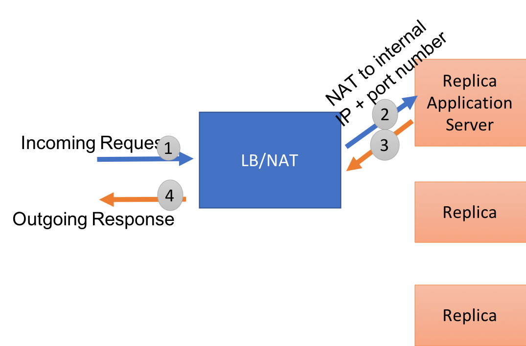
Attack target: First, consider a tenant with a number of replica application servers (replicas). Its baseline reaction to DDoS attacks or flash crowds is to autoscale the replicas (automatically increase their number). The server/client loads could be balanced by round-robin DNS or via a Load Balancer (LB). The LB could act as an (inline) Network Address Translator (NAT) or redirect sessions to the replicas. A tenant could have multiple LBs via round-robin DNS. Also, a tenant could have a layer of indirection servers (proxies) between the LB(s) and replicas, and, again, the LB(s) could either NAT, see Figure 1, or redirect sessions to the proxies.

Figure 1: Baseline tenant with LB/NAT and no proxies.

We herein consider a tenant that services a plurality of clients with a plurality of replicas. DNS resolves clients’ session requests to the tenant’s LB. The LB redirects session request to a proxy, i.e., the LB is not a NAT. Clients contact their proxies directly and do not know the address of their replica server. See Figure 2. The tenant will have a coordination server that will, in particular, control the DNS records of LBs and proxies, and the NAT from proxies to replicas. Load-balanced content distribution networks (CDNs) or session establishment systems are examples adaptable to this architecture.

Each replica can be reached from plural proxies (by proxy-to-replica NAT). Though a volumetric DDoS attack would typically overwhelm the proxies before the LB, i.e., the LB would not be the bottleneck, the proxies may shield the replicas.

Figure 2: LB-to-proxy redirection.

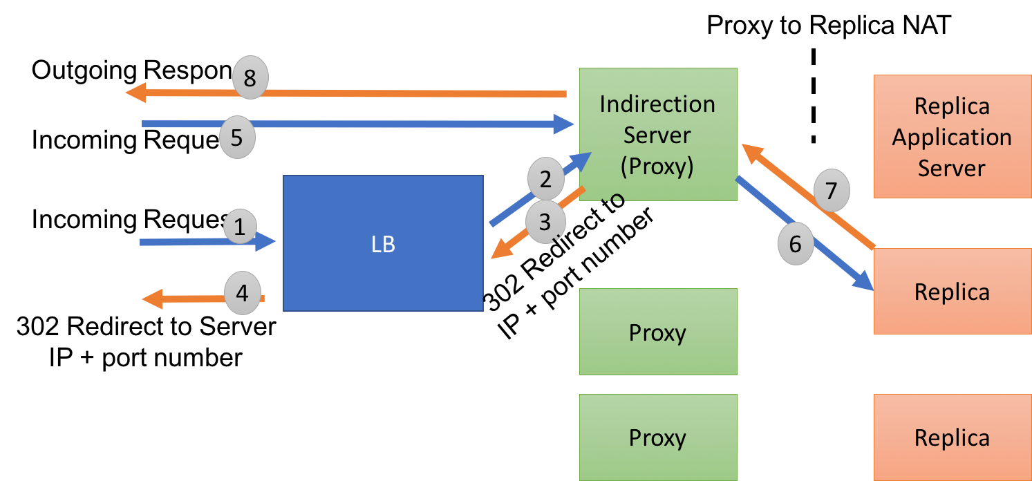
LB-to-proxy redirection: The proposed defense requires LB-to-proxy session redirection. LB-to-proxy redirection by proxy domain name requires that clients obtain proxy (IP, port number) by DNS (note that DNS cannot be used to implement NAT). Otherwise, if redirection is by proxy (IP, port number), then nominal clients need to obtain the proxy’s domain name by reverse DNS for HTTPS (web servers associate SSL certificates to domain names). There is increased attacker workfactor if redirection is by proxy domain name because a bot needs to query DNS before flooding the proxy; note that flooding bots don’t care about SSL certificates. If the LB redirects to proxies by both proxy (IP, port number) and domain name, then additional DNS querying by the client may not be required for redirection, and proxy DNS records would only need to be stored locally by coordination server and LB; but this would be a change to the HTTP redirection mechanism. Unlike previous work that has suggested changes to SSL/TLS, e.g., changes to TLS to support middleboxes [13], these proposed changes are the minimum required to streamline hot server migration.

This paper is organized as follows. In Section II, we motivate and describe the proactive moving-target defense. In Section III, we briefly describe an “adversarial” coupon-collection model for botnet reconnaissance of proxies under moving-target (motag) defense. In Section IV, we describe our AWS emulations and give example results. These results are compared against an adversarial coupon-collection model allowing extrapolation to larger-scale scenarios. After a brief summary in in Section V and acknowledgements, the paper concludes with an Appendix on adversarial coupon collection models.

II Proactive Moving-Target (motag) Defense against Reconnaissance by Changing LBs and Proxies

Under our proposed motag defense, the LB may change its IP periodically via DNS (if plural LBs under round-robin DNS, then the set of LB IPs periodically change). Proxies age-out and are replaced by new ones with different IPs. Proxy Virtual Machines (VMs) of the same tenant need to be on different physical servers, i.e., different proxies have different IPs (different VMs on a physical server are discriminated by port numbers). So, a flood targeting tenant X’s proxy may have collateral damage on other tenants’ VMs sharing the same physical server, but not on other proxies of tenant X. Active clients of proxies aging-out will redirect to the LB. Note that it’s possible that redirection could be initiated by the aging-out proxy, depending on the application. Inactive proxy or LB identities time-out and are then blackholed for a long time (longer for proxy identities). It’s possible that a client’s replica does not change during redirection (e.g., AWS elastic IP), again depending on the application. See Figure 3.

Redirecting persistent HTTP connections [4] via the HTTP REDIRECT command requires tearing down the current TCP connection and establishing a new one between the client and the new server, which can result in some service interruptions. As another example, redirecting streamed-media sessions under RTSP [16] requires an RTSP TEARDOWN and RTSP SETUP to establish the new RTSP session with the new server. Additionally, the control and streaming connections over UDP (RTCP and RTP connections respectively) need to be setup with the new server.

The tenant’s coordination server can also selectively or randomly decide which individual proxy to change, e.g., by selecting those experiencing a sufficiently high number of half-opened TCP sessions and so are likely being actively reconnoitered. Alternatively, all proxies can change simultaneously and periodically.

In the following, we assume that a subpopulation of bots engages in continual, active reconnaissance of the current proxy identities and then targets the rest of the botnet prior to launching the DDoS attack. Again, this assumption is well motivated when the majority of (IoT based) bots cannot cope with redirection. Note that botnets are known to periodically observe the target during an attack to assess its impact.

Figure 3: Proxy-to-proxy redirection.

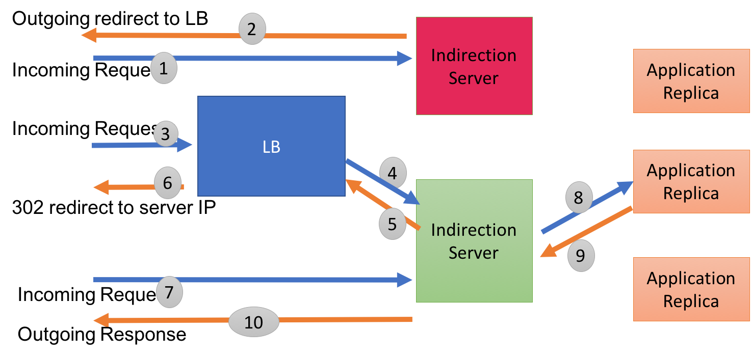
Whether proxy-to-proxy redirection: Suppose there is no proxy-to-proxy redirection so that an “aged-out” (not “current”) proxy no longer takes new sessions and can be deactivated/removed once all of its sessions time out. So, more active proxies are maintained at greater cost than under proxy-to-proxy redirection. This may be a minor additional cost when client sessions are short.

Anonymous reconnaissance: Botnet reconnaissance of LBs or proxies could involve TOR for anonymity and increased apparent source diversity, but TOR is often used for vulnerability scanning and its exit routers may be blacklisted. A botnet could also use more costly VPNs for anonymity, but they don’t give increased source diversity from the attack-target’s point of view. Increased source diversity could also be achieved behind dynamic DNS service.

Previous related work: In [2, 3], similar moving-target defenses involved shuffling server addresses. For a system without proxies, they focus on detecting a vulnerable server (i.e., vulnerability probing not reconnaissance to identify all servers). In their threat model, the attacker essentially samples servers “with replacement” leading to a simple binomial-distribution model; see Section III and the Appendix for models based on Stirling numbers of the second kind.

Detection of active reconnaissance. The proxies may detect active reconnaissance by standard means, e.g., by counting over a sliding time-window the number of half-opened TCP sessions, failed login attempts, and/or successful log-ins/sessions by a single client as in a client reputation system. A client reputation system can also be informed by detected mock sessions (after successful log in). However, a client reputation system would be undermined by the attacker’s use of anonymity services.

II-A Summary increased attacker workfactors

Targeting the LBs: Under LB motag, a flooding bot needs to periodically query DNS to ensure its attack is not targeting a now blackholded IP. But frequent queries by the same source IP for the same domain name is an attack signature that is easy to detect. A smaller number of randomly selected more powerful bots can query DNS for the current LB IPs, possibly via an anonymization service, and once the current LB IPs have been captured, the rest of the botnet is targeted. If the flooding bots target the LBs and the LBs are overwhelmed, the tenant can autoscale the number of LBs.

Targeting the proxies: If the LB is (or LBs are) not overwhelmed, the bots could simply retarget their flood to the proxies when redirected. But some IoT-based bots may not be able to cope with the LB-to-proxy or proxy-to-proxy redirection (even if redirection is by IP + port number). Fewer, powerful bots may be able to mount long realistic sessions and follow redirection, but such sessions may be detected or timed-out, and a periodic retargeting phase is still needed. Alternatively, a subpopulation of bots can repeatedly query DNS for current LBs and retarget the rest of the botnet by collected proxies’ (IP, port number) identities. This kind of botnet reconnaissance is the focus of the following. As for LBs, the target can be further diffused by reactive autoscaling the number of proxies.

II-B Summary overhead on the nominal clients

Nominal clients need to deal with the overhead and quality of service degradation associated with redirection, possibly including additional DNS transactions. For example, nominal clients of streaming media service, including live video broadcast, may not experience significant service degradation because their (initially primed) playout buffers can tolerate transmission interruptions due to redirection. Clients of more interactive sessions, especially real-time sessions whose dataplane travels through the cloud, may experience some service interruption due to redirection.

To illustrate this, consider the video clips we have posted here [12] for the case of RTSP redirection [16] of video streaming servers. The clips were created by simply running two servers (port numbers 1051 or 1052 indicated at bottom of the display) and a client video player, all on a single desktop computer. A different clip is shown for cases with or without a client playout buffer, the former modeling streaming and latter modeling interactive video (as in gaming). The server changes are indicated by port changes (“STREAMING FROM”): $1051\rightarrow 1052$ or $1052\rightarrow 1051$. Video playback noticeably stalls longer upon redirection without a playout buffer than with a 200-frame (5 second) playout buffer. For this and other types of interactive applications, customized techniques have been developed (e.g., predictive prefetching) to try to improve user experience during redirection.

II-C Summary direct tenant costs of motag defense

Regarding the tenant’s costs, consider again the “baseline” tenant of Figure 1. Compared to the baseline tenant, the proposed motag defense has additional costs for the proxy VMs themselves and for reactive autoscaling. Autoscaling proxies may be cheaper than LBs (LBs may be mounted on physical routers) and replicas (replicas would need larger VMs for computationally intensive applications). Obviously, motag defense has costs associated with swapping one proxy VM (or LB) for another. Note that external network IO costs associated with replicas of the baseline tenant are instead borne by proxies under motag defense.

III Coupon-collector model of botnet reconnaissance and moving-target defense

We relate the problem of botnet reconnaissance of the current set of moving-target proxies to an “adversarial” coupon-collector problem where

• the adversary is the coupon collector,

• coupons selection (at mean rate $\beta$) correspond to probing bots assigned to current proxies, and

• each proxy server corresponds to a different coupon type ($m$ in total).

It’s the objective of the collector (botnet) to select coupons so that one of every current type is obtained before the coupon types are changed (at mean rate $\delta$).

Assume that the length of time between successive changes in the $m$ types of coupons (proxies) is exponentially distributed with mean $1/\delta$, a memoryless distribution with high variance (which may be advantageous since a deterministic time may be more easily learned, and anticipated, by the attacker). So, all $m$ coupon types are periodically changed according to an independent Poisson process with rate $\delta$.

Consider a coupon collector (probing botnet) that selects coupons from the set of $m$ coupon types uniformly at random (with replacement) at aggregate rate $\beta$. When the $m$ coupon types all change, the collector starts over with zero.

Let $\rho=\beta/\delta$.

Proposition 1

Under deterministically periodic coupon-selection and Poisson coupon-type changing processes, the stationary mean number of different currently valid coupons obtained is

$$1/(\mbox{e}^{1/\rho}-(1-1/m)).$$

Proposition 2

Under independent Poisson coupon-selection (rate $\beta$) and coupon-type changing (rate $\delta$) processes, the stationary mean number of different currently valid coupons obtained (from a maximum of $m$) is

$$m\frac{\rho}{m+\rho}=m\frac{\beta}{m\delta+\beta}.$$

Note that these two results are close for large $\rho$ since $\mbox{e}^{1/\rho}\sim 1+1/\rho$ as $\rho\rightarrow\infty$.

The proofs of Propositions 1 and 2 and additional related results on adversarial coupon collection are given in the Appendix. These results represent two extremes in the way the botnet may probe for currently valid proxy identities - inter-probe times that are exponentially distributed (high variance) or constant-rate probing (zero variance), cf., comparable figures between Tables I and II.

We next show how accurate such models are with regard to our AWS emulations and use them to extrapolate to larger-scale scenarios.

IV Performance of AWS prototype

IV-A Experimental set-up

On AWS, we set-up HTTP sessions between users and replicas - specifically, Apache web servers with a PHP shopping cart application that interacts with a MySQL database (essentially the LAMP stack). All proxies reside in containers that are spun up ahead of planned proxy address change (again, this may not be needed if a service like AWS elastic IP is used).

For our emulation results described below, the mean time between probes by each reconnoitering bot was 30s, and the time between proxy-identity changes (all proxies change identities and at the same times) had mean 30s. Assignment of proxies to bots is either randomized or round-robin, the latter requiring emulation of the session setup process of nominal clients.

IV-B Emulation results

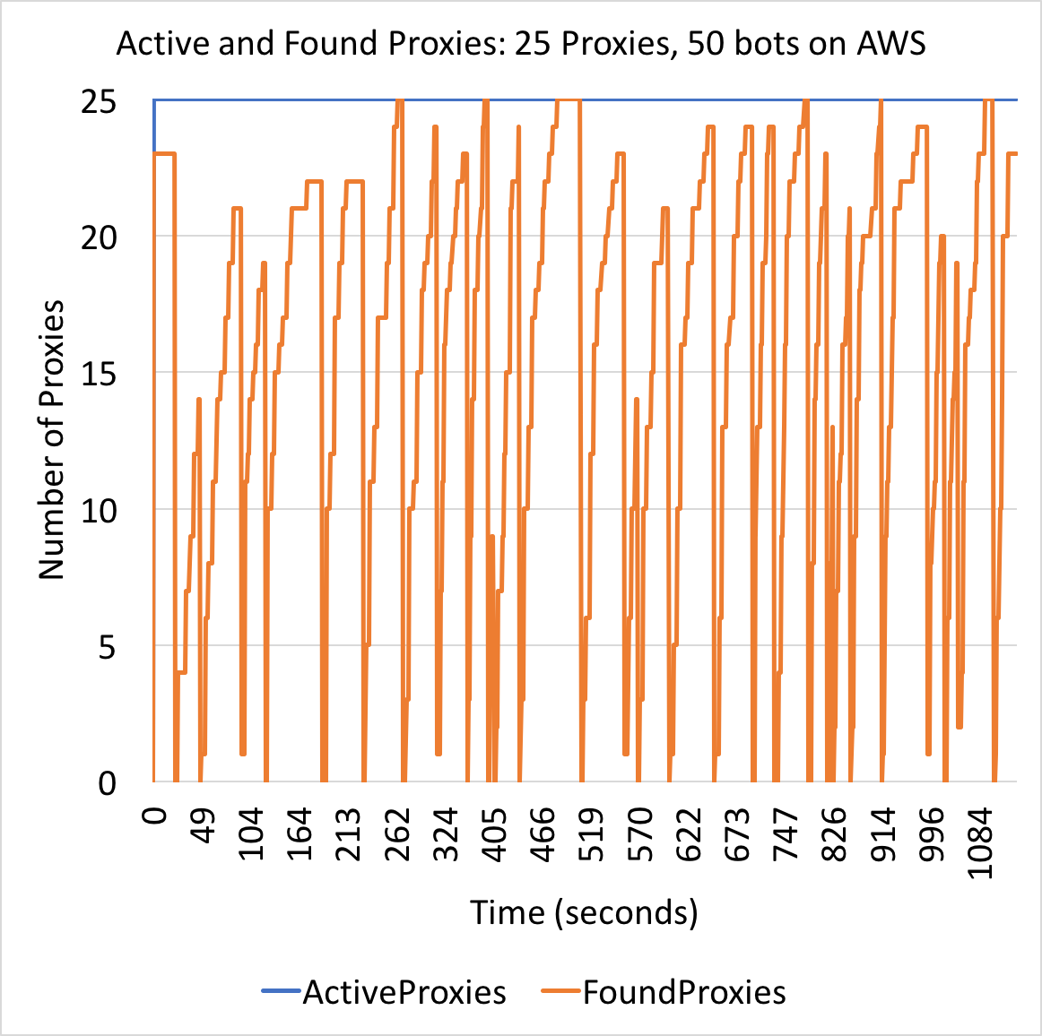
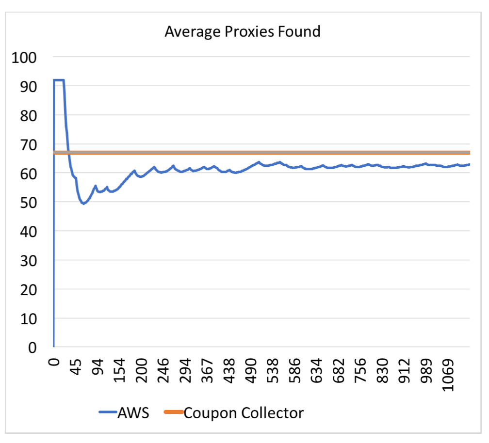
A typical experimental result from our AWS emulations is given in Figs. 4 and 5 for: $m=25$ proxies; $50$ bots each with mean of the exponentially distributed inter-probe time $30$ seconds so that the total mean probing rate was $\beta=50/30$; and the mean of the exponentially distributed time between successive proxy identity changes is $30$ seconds so $\delta=1/30$. Thus, $\rho=\beta/\delta=50$. Note that, generally, $\beta$ (and hence $\rho$) may be roughly proportional to the number of probing bots. Finally, randomly chosen proxies are assigned to probes from the bots.

Figure 4: Number of current proxies identities known to the botnet over time with $m=25$, $\rho=50$.

Figure 5: Running time-average number of current proxies identities known to the botnet with $m=25$, $\rho=50$.

Table I compares the results of the AWS emulations, coupon-collector model of Prop. 2.

method  $\backslash$  $m,\rho$	25,5	25,25	25,50
AWS emulations	16%	48%	62%
coupon collector (Prop. 2)	17%	50%	67%

TABLE I: Stationary mean percentage of proxies known to the botnet under Poisson proxy changes and probing

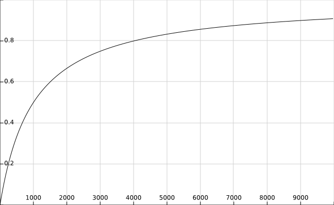
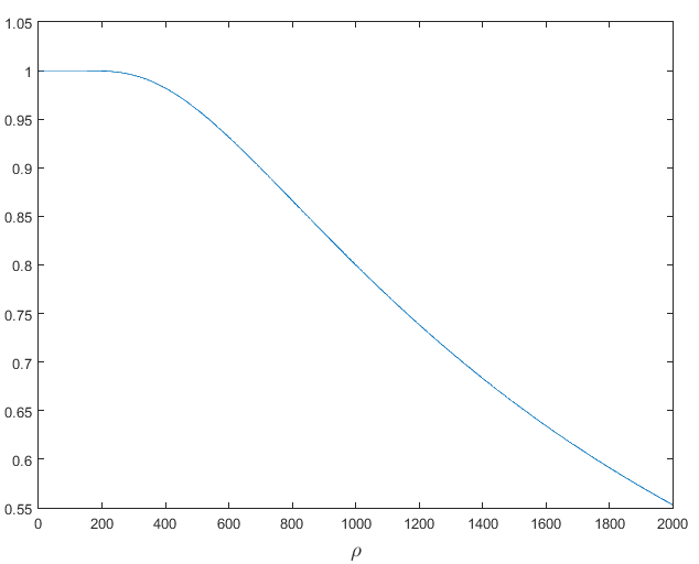
In Fig. 6, we use the coupon collector model of Prop. 2 to extrapolate to the case of $m=1000$ servers. In Figure 7, we use the distribution for the Poisson (exponential) probing case (see Proposition 3 in the Appendix) to plot the probability that at least 20% of the servers are not found as a function of $\rho$.

Figure 6: The average fraction of proxies known to the botnet as a function of $\rho=\beta/\delta$ for $m=1000$ proxies.

Figure 7: The probability that at least 20% of proxies are not found for $m=1000$ servers under Poisson probing.

method  $\backslash$  $\kappa$	.05	.25	.5
AWS emulations	67.3%	66.8%	54.6 %

TABLE II: Mean percentage of proxies known to the botnet under deterministic probing with $m=25,\rho=50$ under “truncated” Gaussian interprobing times

For Table II, we instead use truncated Gaussian distributed inter-probe times lower bounded by 2 seconds. Here, the variance of inter-probe times is taken smaller than under the exponential distribution considered above. The low-variance case $\kappa=0.05-0.25$ is very close to 67.1% given by Prop. 1 for deterministic-rate probing. To see why, note that because $\beta\gg\delta$ ($\rho\gg 1$) in this case, there are typically many probes over the time $T$ between proxy address changes (${\sf E}T=1/\delta$); so, with low-variance inter-probe times, by the law of large numbers one would continue to expect the number of probes to likely be about $\beta T$ as for constant probing, see the Appendix. About $2/3$ of the proxies are known to the botnet on average in steady-state (i.e., about $1/3$ would be available for nominal clients during the attack) when $m=25,\rho=50$ for both deterministic and Poisson probing, which is a lot greater than under higher-variance Gaussian probing, cf., (VI-B3) of the Appendix. Other relevant models of coupon collection are considered in the Appendix, e.g., where individual proxies change independently rather than collectively.

V Summary

In this paper, we considered a botnet intending to launch at DDoS attack against a tenant of the public cloud. We motivated how a tenant whose clients are redirected to a bank of proxy servers that periodically change compels a botnet to actively probe the tenant to determine a set of currently valid proxy identities for targeting purposes. The performance of this moving-target defense against botnet reconnaissance was studied by AWS emulations and by adversarial coupon-collection models to show how, at any given time, a certain number of proxies are not known to the botnet and would be available to nominal clients during the DDoS attack. Those servers will continue to be available to the community of nominal clients even after the rest of the botnet is targeted and the DDoS attack is launched.

VI Appendix: Adversarial coupon-collector models

We consider a coupon-collector problem involving an adversary. In a cyber security interpretation, the collector is the attacker targeting a bank of servers and its adversary is the defender. That is, suppose bots of a bot network (botnet) are conducting reconnaissance on the servers by selecting one at random and communicating with it in order to identify it. The servers protect against reconnaissance by periodically changing their identities. So that the botnet cannot anticipate when server identities change, we assume that times between these events are independent and (memorylessly) exponentially distributed. Thus the bots need to continually sample the servers to capture their current identities.

In terms of coupon collection, assume that there is a coupon collection process and that, periodically, the coupon types are replaced so that the collector needs to start over. There are $m$ different types of coupons independently chosen uniformly at random. Let $Y\leq m$ be the process representing the number of different coupon types possessed by the collector and $K$ (or $K(T)$) be the number of coupons selected in the interval $T$ between coupon-type replacements. We develop continuous-time models in the following using Stirling numbers of the second kind and an associated distribution. In Table III, we give the correspondence between this cyber security and the coupon collector model.

cyber defense context	coupon collector context	parameter
reconnaissance attack	coupon selection	rate $\beta$
server/target	coupon type	$m$ types
defense	change coupon type	rate $\delta$

TABLE III: Cyber defense and coupon collector jargon correspondence

This Appendix is organized as follows. In Section VI-A, we give some background on Stirling numbers of the second kind. In Section VI-B, we consider models where periodically all coupon types are changed at the same time. In Section VI-C, we consider models where periodically coupon types are selectively replaced independently.

VI-A Background on Stirling Numbers of the Second Kind

Given coupons of $m$ different types. If $k$ distinct coupons are independently selected, the number of ways of selecting $y\leq k\wedge m:=\min\{k,m\}$ distinct types is

$$\frac{m!}{(m-y)!}{k\brace r}, {k\brace y}=\frac{1}{y!}\sum_{j=0}^{y}(-1)^{y-j}\binom{y}{j}j^{k}$$ where

is a Stirling number of the second kind. Assuming that the type of a selected coupon is equally likely any of the $m$ types, the probability that $k$ distinct coupons are selected so that $y$ of $m$ distinct types result is

$$P_{m,k}(y) := \frac{\frac{m!}{(m-y)!}{k\brace y}}{m^{k}}$$ (1)

where

$$m^{k} = \sum_{y=1}^{k\wedge m}\frac{m!}{(m-y)!}{k\brace y},~{}y\in\{1,2,...,k\wedge m\},$$

see Equation (1.55) of [8]. Note that this discrete distribution $P_{m,k}$ is different from the “Stirling distribution of the second kind” (Equation (4.98) of [8]).

From, e.g., (1.94c) on p. 82 of [18], we have that the power series

$$\sum_{k=0}^{\infty}{k\brace\ell}x^{k+1}=\frac{1}{(1/x)_{\ell+1}},$$ (2)

where $(a)_{\ell}:=a(a-1)(a-2)\cdots(a-\ell+1)$.

For numerical computations, we can employ known asymptotic approximations of the Stirling numbers of the second kind. For example, if $\ell$ is fixed then ${k\brace\ell}\sim\ell^{k}/\ell!$ as $k\rightarrow\infty$, see 26.8.42 at [14] (also see [19, 11]). Then using logarithms, we can compute the distributions $P_{m,k}$. When $k\gg m$ or $k\ll m$, the distribution $P_{m,k}(\cdot)$ is concentrated at its mode very near $k\wedge m$. However when $k=m$, the mode is about 20-25% less than the maximum (at $k=m$).

VI-B Periodically replacing all coupon types

VI-B1 Deterministic coupon selections with Poisson coupon-type replacements

Proposition 1

Under constant rate coupon-selection (constant rate $\beta$), and Poisson coupon-changing process (mean rate $\delta$) determining when all coupon types are replaced, the stationary mean number of currently valid, different coupon types obtained is

$${\sf E}Y = \frac{1}{\mbox{e}^{1/\rho}-(1-\frac{1}{m})}.$$ (3)

Proof: At constant $\beta$ selections/s, the number of coupons selected over $[0,T]$ is simply

$$K = [\beta T].$$

$K$ is a geometric random variable,

$${\sf P}(K=k)={\sf P}(k/\beta\leq T<(k+1)/\beta)=\mbox{e}^{-k/\rho}\bigg{(}1-\mbox{e}^{-1/\rho}\bigg{)},$$

for $k=0,1,2\ldots$, with probability generating function

$${\sf E}z^{K}=\frac{1-\mbox{e}^{-1/\rho}}{1-z\mbox{e}^{-1/\rho}}.$$

So,

$${\sf E}Y={\sf E}m(1-(1-\frac{1}{m})^{K})=\frac{\mbox{e}^{-1/\rho}}{1-(1-\frac{1}{m})\mbox{e}^{-1/\rho}}~{},$$

which is (3). Since Poisson Arrivals See Time Averages (PASTA) [20, 1], this is also the expected number of different types of coupons collected at a typical time. ∎

VI-B2 Poisson coupon selection with independent Poisson coupon-type replacement process

Proposition 2

Under Poisson coupon-selection (rate $\beta$), Poisson coupon-changing process (rate $\delta$), the stationary mean number of currently valid, different coupon types obtained is

$${\sf E}Y = m\frac{\rho}{m+\rho}.$$ (4)

Proof: The number of coupon types collected just before coupon types are replaced is

$${\sf E}m(1-(1-1/m)^{K}).$$

Conditioning on $T$, $K\sim{\sf Poisson}(\beta T)$. So, the mean number of different coupons obtained conditioned on $T$ is simply

$$\sum_{k=0}^{\infty}m(1-(1-1/m)^{k})\frac{(\beta T)^{k}\mbox{e}^{-\beta T}}{k!}=m(1-\mbox{e}^{-\beta T/m}).$$ (5)

Using the moment generating function of $T\sim\exp(\delta)$, we get

$${\sf E}m(1-(1-1/m)^{K}) = {\sf E}m(1-\mbox{e}^{-\beta T/m})$$

$$= m\left(1-\frac{\delta}{\delta+\beta/m}\right)$$

which is (4). Finally, since PASTA, this is also the expected number of different coupons collected at a typical time. ∎

Note that (4) and (3) are close when $\rho$ is large since $\mbox{e}^{1/\rho}\sim 1+1/\rho$.

Also note that when $m\gg\rho$, the expected number of different coupons in steady state is approximately $\rho$ which has nothing to do with $m$. On the other hand, if $\rho\gg m$, all $m$ coupons are likely collected following intuition.

Proposition 3

Under Poisson coupon-selection (rate $\beta$) and Poisson coupon-changing process (rate $\delta$), in steady state,

$${\sf P}(Y=\ell)=\frac{1}{\rho}\,\frac{m}{m-\ell}\,\,\frac{m}{m\frac{\rho+1}{\rho}}\,\frac{m-1}{m\frac{\rho+1}{\rho}-1}\cdots\frac{m-\ell}{m\frac{\rho+1}{\rho}-\ell},$$

for $1\leq\ell\leq m$.

Proof: Again, $K$ given $T$ is $\sim{\sf Poisson}(\beta T)$. The unconditional distribution of $K$ is geometric:

$${\sf P}(K(T)=k) = \int_{0}^{\infty}\delta\mbox{e}^{-\delta t}\frac{(\beta t)^{k}\mbox{e}^{-\beta t}}{k!}\mbox{d}t$$ (6)

$$= \bigg{(}\frac{\rho}{\rho+1}\bigg{)}^{k}\,\frac{1}{\rho+1},\quad k\geq 0$$

Thus, for $\ell\in\{0,1,...,m\}$,

$${\sf P}(Y(K(T))=\ell) = \sum_{k=0}^{\infty}{\sf P}(Y(k)=\ell)\bigg{(}\frac{\rho}{\rho+1}\bigg{)}^{k}\frac{1}{\rho+1}$$

$$= \sum_{k=0}^{\infty}\frac{(m)_{\ell}}{m^{k}}{k\brace\ell}\bigg{(}\frac{\rho}{\rho+1}\bigg{)}^{k}\frac{1}{\rho+1}$$

$$= \frac{(m)_{\ell}}{\rho+1}\frac{\rho+1}{\rho/m}\sum_{k=0}^{\infty}{k\brace\ell}\bigg{(}\frac{\rho/m}{\rho+1}\bigg{)}^{k+1}$$

$$= \frac{m}{\rho}\,(m)_{\ell}\frac{1}{\bigg{(}\frac{\rho+1}{\rho/m}\bigg{)}_{\ell+1}}$$

where the last equality is (2). Again since PASTA, this is the steady-state distribution of the number of coupon types obtained. ∎

See the Markov chain below with transition rates (10) and (11) and parameter $r=1$.

VI-B3 Discussion: Renewal coupon selections, Poisson coupon-type replacements

Suppose that the coupon selection process $K(t)$ is a renewal counting process with interarrival times $X$ of finite variance, $\sigma^{2}<\infty$, and mean $1/\beta$. The classical central limit theorem for renewal processes is (e.g., [5]),

$$\lim_{t\rightarrow\infty}{\sf P}\left(\frac{K(t)-\beta t}{\sqrt{\sigma^{2}\beta^{3}t}}<y\right) = \frac{1}{\sqrt{2\pi}}\int_{-\infty}^{y}\mbox{e}^{-z^{2}/2}\mbox{d}z,$$

i.e., $K(t)\sim{\sf N}(\beta t,\sigma^{2}\beta^{3}t)$ as $t\rightarrow\infty$. We can consider a regime where $\delta^{-1}\gg\beta^{-1}$ ($\rho\gg 1$) so that this is approximately valid for $K(T)$ when $T\sim\exp(\delta)$. Let $v=-\log(1-1/m)>0$. Using the MGF of a Gaussian, we can approximate the expected number of different coupon types collected just before they’re replaced as:

$${\sf E}m(1-(1-1/m)^{K(T)}) \sim {\sf E}m(1-\mbox{e}^{-\beta Tv+\sigma^{2}\beta^{3}Tv^{2}/2})$$

as $$\rho=\beta/\delta\rightarrow\infty$$

$$= m\left(1-\frac{\delta}{\delta+\beta v-\sigma^{2}\beta^{3}v^{2}/2}\right)$$

requiring $\delta+\beta v-\sigma^{2}\beta^{3}v^{2}/2>\delta$, i.e., $\beta^{-1}>\sigma\sqrt{v/2}$. That is, when $\rho=\beta/\delta$ is large, there are obviously many coupons selected before the coupon types are changed. Again since PASTA, this is the stationary number of different coupon-types collected. When $\sigma=0$, this limit agrees with the deterministic coupon selection (3) of Proposition 1 when $m$ and $\rho$ are large since $v\sim 1/m$ and $\mbox{e}^{1/\rho}\sim 1+1/\rho$.

VI-C Individual coupon types independently replaced at random, according to a single Poisson process

Consider the discrete-time Markov chain $Y(k)$ satisfying

$$Y(k) = Y(k-1)+\xi_{k},\quad k\geq 1,$$

where $Y(0)\in\{0,1,2,...,m\}$ (i.e., $Y(0)$ is not necessarily zero a.s.) and

$${\sf P}(\xi_{k}=0|Y(k-1),\ldots,Y(0)) = \frac{Y(k-1)}{m},$$

$${\sf P}(\xi_{k}=1|Y(k-1),\ldots,Y(0)) = 1-\frac{Y(k-1)}{m}.$$

Here, $Y(k)$ is the number of different types of coupons collected after the $k^{\rm th}$ coupon selection including those initially had, $Y(0)$.

VI-C1 Verifying (4) when $Y(0)=0$ a.s.

We can alternatively verify (4) by simply solving the recursion for ${\sf E}Y(k)$ when $Y(0)=0$:

$${\sf E}Y(k) = 1+(1-\frac{1}{m})+(1-\frac{1}{m})^{2}+\cdots+(1-\frac{1}{m})^{k-1}$$

$$= m\bigg{(}1-(1-\frac{1}{m})^{k}\bigg{)}.$$

Note that $Y(0)=0$ a.s. implies $\xi_{1}=1$ a.s. Now let us collect coupons at the ticks of a Poisson process $K(t)$, $t\geq 0$, with rate $\beta$ and independent coupon types selected independently and uniformly. Thus, at real time $t\geq 0$, we have collected

$$Y(K(t))~{}\text{ different types of coupons}.$$

So,

$${\sf E}(Y(K(t))) = \sum_{k=0}^{\infty}m\bigg{(}1-(1-\frac{1}{m})^{k}\bigg{)}{\sf P}(K(t)=k)$$

$$= m(1-e^{-\beta t/m}).$$

So if $t=T$ is exponentially distributed with rate $\delta$,

$${\sf E}(Y(K(T))) = \int_{0}^{\infty}m(1-e^{-\beta t/m})\delta e^{-\delta t}\mbox{d}t$$

$$= \frac{m\rho}{m+\rho}.$$

VI-C2 Independent coupon-type replacements, $Y(0)\not\equiv 0$ a.s.

A generalization of (4) is:

Proposition 4

For Poisson coupon selection (at rate $\beta$), Poisson coupon-type replacements (at rate $\delta$), and individual coupon types are independently replaced with probability $r$, the mean number of valid coupon types obtained in steady state is

$$m\frac{\rho}{rm+\rho}$$ (8)

Proof: For $Y(0)\not\equiv 0$ a.s., solving the recursion

$${\sf E}Y(k) = {\sf E}Y(k-1)-{\sf E}\xi_{k}~{}=~{}1+(1-1/m){\sf E}Y(k-1)$$

gives, for $k\geq 1$,

$${\sf E}Y(k) = 1+(1-1/m)+...$$

$$~{}~{}~{}...+(1-1/m)^{k-1}+(1-1/m)^{k}{\sf E}Y(0)$$

$$= m(1-(1-1/m)^{k})+(1-1/m)^{k}{\sf E}Y(0).$$

As above, since $K\sim{\sf Poisson}(\beta T)$ and $T\sim\exp(\delta)$,

$${\sf E}Y(K(T)) = m\frac{\rho}{m+\rho}+\frac{m}{m+\rho}{\sf E}Y(0).$$

In steady-state,

$$(1-r){\sf E}Y(K(T)) = {\sf E}Y(0).$$ (9)

Eliminating ${\sf E}Y(0)$ from the previous two displays gives ${\sf E}Y(K(T))$ equals (8). The proposition follows since PASTA. ∎

Note that when $r=0$ (coupon types are never replaced), the mean number of coupon types obtained in steady-state is $m$.

Here we are modeling the number of coupon types collected as a Markov chain with the following transition rates:

$$q(k,k+1) = \frac{m-k}{m}\beta,~{}~{}0\leq k\leq m$$ (10)

$$q(\ell,k) = \delta\binom{\ell}{k}r^{\ell-k}(1-r)^{k},~{}0\leq k<\ell\leq m$$ (11)

One can find the stationary invariant distribution $\pi$ through the balance equations, $\pi^{\rm T}q=0$. For $r=1$, this stationary invariant $\pi$ is that of Proposition 3.

VI-C3 Individual coupon types replaced according to independent Poisson processes

A simpler variation is one in which each coupon is reset according to an independent Poisson process at rate $\delta$. Here, the upward transition rates are (10) but, instead of (11), the downward transition rates are

$$q(\ell,\ell-1)=\delta\ell,~{}~{}1\leq\ell\leq m.$$

So, this is a birth-death Markov process. Here, a separate $\sim\exp(\delta)$ clock would be required to reset each coupon type. The solution of the balance equations is the invariant $\pi$ on $\{0,1,2,...,m\}$:

$$\pi(k) = \pi(0)\prod_{j=1}^{k}\frac{q(j-1,j)}{q(j,j-1)}$$

$$= \pi(0)\binom{m}{k}\left(\frac{\rho}{m}\right)^{k},$$

where $\pi(0)$ is chosen so that $\sum_{k=0}^{m}\pi(k)=1.$

References

- [1] Baccelli, F., and Bremaud, P. Elements of Queueing Theory. Springer-Verlag, Application of Mathematics: Stochastic Modelling and Applied Probability, No. 26, New York, NY, 1991.
- [2] Carroll, T., Crouse, M., Fulp, E., and Berenhaut, K. Analysis of network address shuffling as a moving target defense. In Proc. IEEE ICC (2014).
- [3] Crouse, M., Prosser, B., and Fulp, E. Probabilistic performance analysis of moving target and deception reconnaissance defenses. In Proc. ACM MTD (Oct. 2014).
- [4] Fielding, R., Gettys, J., Mogul, J., Frystyk, H., Masinter, L., Leach, P., and Berners-Lee, T. Hypertext Transfer Protocol – HTTP/1.1. IETF RFC 2616 (June 1999, https://www.ietf.org/rfc/rfc2616.txt).
- [5] Gallager, R. Renewal Processes. http://www.rle.mit.edu/rgallager/documents/Renewal.pdf.
- [6] Hansson, L., Hogh, P., Bachmann, B., Jorgensen, K., and Rand, D. The BlackNurse Attack. http://soc.tdc.dk/blacknurse/blacknurse.pdf, 2016.
- [7] Hilton, S. Dyn Analysis Summary of Friday October 21 Attack. http://dyn.com/blog/dyn-analysis-summary-of-friday-october-21-attack/, Oct. 26, 2016.
- [8] Johnson, N., Kemp, A., and Kotz, S. Univariate Discrete Distributons, 3rd ed. Wiley, Aug. 2005.
- [9] Krebs, B. The Democratization of Censorship. http://krebsonsecurity.com/tag/ddos/, Sept. 16, 2016.
- [10] Kumar, M. Biggest-Ever DDoS Attack (1.35 Tbs) Hits GitHub Website. https://thehackernews.com/2018/03/biggest-ddos-attack-github.html, March 1, 2018.
- [11] Louchard, G. Asymptotics of the Stirling numbers of the second kind revisited. Appl. Anal. Discr. Math. 7, 2 (2013), 193–210.
- [12] Nasiriani, N. RTSP video server and client with RTSP REDIRECT compatibility. https://github.com/neda824/RTSP-Video-Server-Client.
- [13] Naylor, D., Schomp, K., Varvello, M., Leontiadis, I., Blackburn, J., Lopez, D., Papagiannaki, K., Rodriguez, P., and Steenkiste, P. Multi-Context TLS (mcTLS): Enabling Secure In-Network Functionality in TLS. In Proc. ACM SIGCOMM (London, Aug. 2015).
- [14] NIST. Digital library of mathematical functions. http://dlmf.nist.gov/26.8#vii.
- [15] RTSP Client Server. https://github.com/mutaphore/RTSP-Client-Server.
- [16] Schulzrinne, H., Rao, A., and Lanphier, R. Real Time Streaming Protocol. IETF RFC 2326 (April 1998, https://www.ietf.org/rfc/rfc2326.txt).
- [17] http-slowloris. https://nmap.org/nsedoc/scripts/http-slowloris.html.
- [18] Stanley, R. Enumerative Combinatorics, 2nd ed., vol. 1. Cambridge, 2011.
- [19] Temme, N. Asymptotic estimates of Stirling numbers. Stud. Appl. Math. 89, 3 (1993), 233–243.
- [20] Wolff, R. Stochastic Modeling and the Theory of Queues. Prentice-Hall, Englewood Cliffs, NJ, 1989.