Model independent constraints on transition redshift

Abstract

This paper aims to put constraints on the transition redshift $z_{t}$, which determines the onset of cosmic acceleration, in cosmological-model independent frameworks. In order to perform our analyses, we consider a flat universe and assume a parametrization for the comoving distance $D_{C}(z)$ up to third degree on $z$, a second degree parametrization for the Hubble parameter $H(z)$ and a linear parametrization for the deceleration parameter $q(z)$. For each case, we show that type Ia supernovae and $H(z)$ data complement each other on the parameter space and tighter constrains for the transition redshift are obtained. By combining the type Ia supernovae observations and Hubble parameter measurements it is possible to constrain the values of $z_{t}$, for each approach, as $0.806\pm 0.094$, $0.870\pm 0.063$ and $0.973\pm 0.058$ at 1$\sigma$ c.l., respectively. Then, such approaches provide cosmological-model independent estimates for this parameter.

I Introduction

The idea of a late time accelerating universe is indicated by type Ia supernovae (SNe Ia) observations SN1 ; SN2 ; SN3 ; SN4 ; SN5 ; union ; union2 ; union21 and confirmed by other independent observations such as Cosmic Microwave Background (CMB) radiation WMAP1 ; WMAP2 ; planck , Baryonic Acoustic Oscillations (BAO) BAO1 ; BAO2 ; BAO3 ; BAO4 ; BAO5 and Hubble parameter, $H(z)$, measurements Omer ; Omer2 ; Omer3 . The simplest theoretical model supporting such accelerating phase is based on a cosmological constant $\Lambda$ term CC ; padmana plus a Cold Dark Matter component reviewDM ; bookDM ; weinberg2013 , the so-called $\Lambda$CDM model. The cosmological parameters of such model have been constrained more and more accurately planck ; Omer2 ; sharov as new observations are added. Beyond a constant $\Lambda$ based model, several other models have been also suggested recently in order to explain the accelerated expansion. The most popular ones are based on a dark energy fluid peebles ; sahni2 endowed with a negative pressure filling the whole universe. The nature of such exotic fluid is unknown, sometimes attributed to a single scalar field or even to mass dimension one fermionic fields. There are also modified gravity theories that correctly describe an accelerated expansion of the Universe, such as: massive gravity theories volkov , modifications of Newtonian theory (MOND) mond ; mond2 , $f(R)$ and $f(T)$ theories that generalize the general relativity fR ; fR3 ; fR4 , models based on extra dimensions, as brane world models randall ; pomarol ; langlois ; shir ; cline , string string and Kaluza-Klein theories klein , among others. Having adopted a particular model, the cosmological parameters can be determined by using statistical analysis of observational data.

However, some works have tried to explore the history of the universe without to appeal to any specific cosmological model. Such approaches are sometimes called cosmography or cosmokinetic models kine1 ; kine2 ; kine3 ; kine4 ; kine5 ; kine6 , and we will refer to them simply as kinematic models. This nomenclature comes from the fact that the complete study of the expansion of the Universe (or its kinematics) is described just by the Hubble expansion rate $H=\dot{a}/a$, the deceleration parameter $q=-a\ddot{a}/\dot{a}^{2}$ and the jerk parameter $j=-\dddot{a}a^{3}/(a\dot{a}^{3})$, where $a$ is the scale factor in the Friedmann-Roberson-Walker (FRW) metric. The only assumption is that space-time is homogeneous and isotropic. In such parametrization, a simple dark matter dominated universe has $q=1/2$ while the accelerating $\Lambda$CDM model has $j=-1$. The deceleration parameter allows to study the transition from a decelerated phase to an accelerated one, while the jerk parameter allows to study departures from the cosmic concordance model, without restricting to a specific model.

Concerning the deceleration parameter, several studies have attempted to estimate at which redshift $z_{t}$ the universe undergoes a transition to accelerated phase Omer2 ; Omer3 ; kine3 ; cunha2008 ; guimaraes2009 ; Rani2015 ; limajesus2014 ; moresco2016 . A model independent determination of the present deceleration parameter $q_{0}$ and deceleration-acceleration transition redshift $z_{t}$ is of fundamental importance in modern cosmology. As a new cosmic parameter limajesus2014 , it should be used to test several cosmological models.

In order to study the deceleration parameter in a cosmological-model independent framework, it is necessary to use some parametrization for it. This methodology has both advantages and disadvantages. One advantage is that it is independent of the matter and energy content of the universe. One disadvantage of this formulation is that it does not explain the cause of the accelerated expansion. Furthermore, the value of the present deceleration parameter may depend on the assumed form of $q(z)$. One of the first analyses and constraints on cosmological parameters of kinematic models was done by Elgarøy and Multamäki kine5 by employing Bayesian marginal likelihood analysis. Since then, several authors have implemented the analysis by including new data sets and also different parametrizations for $q(z)$.

For a linear parametrization, $q(z)=q_{0}+q_{1}z$, the values for $q_{0}$ and $z_{t}$ found by Cunha and Lima cunha2008 were $q_{0}\sim-0.7$, $z_{t}=0.43^{+0.09}_{-0.05}$ from 182 SNe Ia of Riess et al. SN4 , $-1.17\leq q_{0}\leq−0.16$, $z_{t}=0.61^{+3.68}_{-0.21}$ from SNLS data set SN3 and $-1.0\leq q_{0}\leq−0.36$, $z_{t}=0.60^{+0.28}_{-0.11}$ from Davis et al. data set SN5 . Guimarães, Cunha and Lima guimaraes2009 found $q_{0}=-0.71\pm 0.21$ and $z_{t}=0.49^{+0.27}_{-0.09}$ using a sample of 307 SNe Ia from Union compilation union . Also, for the linear parametrization, Rani et al. Rani2015 found $q_{0}=-0.52\pm 0.12$ and $z_{t}\approx 0.98$ using a joint analysis of age of galaxies, strong gravitational lensing and SNe Ia data. For a parametrization of type $q(z)=q_{0}+q_{1}z/(1+z)$, Xu, Li and Lu Xu2009 used 307 SNe Ia together with BAO and $H(z)$ data and found $q_{0}=-0.715\pm 0.045$ and $z_{t}=0.609^{+0.110}_{-0.070}$. For the same parametrization, Holanda, Alcaniz and Carvalho holanda2013 found $q_{0}=−0.85^{+1.35}_{-1.25}$ by using galaxy clusters of elliptical morphology based on their Sunyaev-Zeldovich effect (SZE) and X-ray observations. Such parametrization has also been studied in kine5 ; cunha2008 .

As one may see, the determination of the deceleration parameter is a relevant subject in modern cosmology, as well as the determination of the Hubble parameter $H_{0}$. In seventies, Sandage sandage foretold that the determination of $H_{0}$ and $q_{0}$ would be the main role of cosmology for the forthcoming decades. The inclusion of the transition redshift $z_{t}$ as a new cosmic discriminator has been advocated by some authors limajesus2014 . An alternative method to access the cosmological parameters in a model independent fashion is by means of the study of $H(z)=\dot{a}/a=-[1/(1+z)]dz/dt$. In the so called cosmic chronometer approach, the quantity $dz$ is obtained from spectroscopic surveys and the only quantity to be measured is the differential age evolution of the universe ($dt$) in a given redshift interval ($dz$). By using the results from Baryon Oscillation Spectroscopic Survey (BOSS) BAO3 ; BAO4 ; BAO5 , Moresco et al. moresco2016 have obtained a cosmological-model independent determination of the transition redshift as $z_{t}=0.4\pm 0.1$ (see also Omer ; Omer2 ; Omer3 ).

In the present work we study the transition redshift by means of a third order parametrization of the comoving distance, a second order parametrization of $H(z)$ and a linear parametrization of $q(z)$. By combining luminosity distances from SNe Ia JLA and $H(z)$ measurements, it is possible to determine $z_{t}$ values in these cosmological-model independent frameworks. In such approach we obtain an interesting complementarity between the observational data and, consequently, tighter constraints on the parameter spaces.

The paper is organized as follows. In Section II, we present the basic equations concerning the obtainment of $z_{t}$ from luminosity distance, $H(z)$ and $q(z)$. Section III presents the data set used and the analyses are presented in Section IV. Conclusions are left to Section V.

II Basic equations

Let us discuss (from a more observational viewpoint) the possibility to enlarge Sandage’s vision by including the transition redshift, $z_{t}$, as the third cosmological number. To begin with, consider the general expression for the deceleration parameter $q(z)$ as given by:

$$q(z)=-\frac{\ddot{a}}{aH^{2}}=\frac{1+z}{H}\frac{dH}{dz}-1\,,$$ (1)

from which the transition redshift, $z_{t}$, can be defined as $q(z_{t})=0$, leading to:

$$z_{t}=\left[\frac{d{\ln}H(z)}{dz}\right]^{-1}_{|_{z=z_{t}}}-1.$$ (2)

Let us assume a flat Friedmann-Robertson-Walker cosmology. In such a framework, the luminosity distance, $d_{L}$ (in Mpc), is given by:

$$d_{L}(z)=(1+z)d_{C}(z),$$ (3)

where $d_{C}$ is the comoving distance:

$$d_{C}(z)=c\int_{0}^{z}\frac{dz^{\prime}}{H(z^{\prime})},$$ (4)

with $c$ being the speed of light in km/s and $H(z)$ the Hubble parameter in km/s/Mpc. For mathematical convenience, we choose to work with dimensionless quantities. Then, we define the dimensionless distances, $D_{C}\equiv\frac{d_{C}}{d_{H}}$, $D_{L}\equiv\frac{d_{L}}{d_{H}}$, $d_{H}\equiv c/H_{0}$ and the dimensionless Hubble parameter, $E(z)\equiv\frac{H(z)}{H_{0}}$. Thus, we have:

$$D_{L}(z)=(1+z)D_{C}(z),$$ (5)

and

$$D_{C}(z)=\int_{0}^{z}\frac{dz^{\prime}}{E(z^{\prime})},$$ (6)

from which follows

$$E(z)=\bigg{[}\frac{dD_{C}(z)}{dz}\bigg{]}^{-1},$$ (7)

From (2) we also have:

$$z_{t}=\left[\frac{d\ln E(z)}{dz}\right]_{|z=z_{t}}^{-1}-1.$$ (8)

Therefore, from a formal point of view, we may access the value of $z_{t}$ through a parametrization of both $q(z)$ and $H(z)$, at least around a redshift interval involving the transition redshift. As a third method we can also parametrize the co-moving distance, which is directly related to the luminosity distance, in order to study the transition redshift. In which follows we present the three different methods considered here.

II.1 $z_{t}$ from comoving distance, $D_{C}(z)$

In order to put limits on $z_{t}$ by considering the comoving distance, we can write $D_{C}(z)$ by a third degree polynomial such as:

$$D_{C}=z+d_{2}z^{2}+d_{3}z^{3}.$$ (9)

where $d_{2}$ and $d_{3}$ are free parameters. Naturally, from Eqs. (7) and (9), one obtains

$$E(z)=\frac{1}{1+2d_{2}z+3d_{3}z^{2}}.$$ (10)

Solving Eq. (8) with $E(z)$ given by (10), we find

$$z_{t}=\frac{-2d_{2}-3d_{3}\pm\sqrt{4d_{2}^{2}-6d_{2}d_{3}+9d_{3}^{2}-9d_{3}}}{9d_{3}},$$ (11)

where we may see there are two possible solutions to $z_{t}$. From a statistical point of view, aiming to constrain $z_{t}$, maybe it is better to write the coefficient $d_{3}$ in terms of $z_{t}$ and $d_{2}$ via Eq. (8) as

$$d_{3}(d_{2},z_{t})=-\frac{1+2d_{2}+4d_{2}z_{t}}{3z_{t}(2+3z_{t})}.$$ (12)

Then

$$E(z)=\left[1+2d_{2}z-\frac{1+2d_{2}+4d_{2}z_{t}}{z_{t}(2+3z_{t})}z^{2}\right]^{-1}.$$ (13)

Finally, from Eqs. (5), (9) and (12) the dimensionless luminosity distance is

$$D_{L}(z)=(1+z)\left[z+d_{2}z^{2}-\frac{1+2d_{2}+4d_{2}z_{t}}{3z_{t}(2+3z_{t})}z^{3}\right].$$ (14)

Equations (14) and (13) are to be compared with luminosity distances from SNe Ia and $H(z)$ measurements, respectively, in order to determine $z_{t}$ and $d_{2}$.

II.2 $z_{t}$ from $H(z)$

In order to assess $z_{t}$ from Eq. (2) by means of $H(z)$ we need an expression for $H(z)$. If one wants to avoid dynamical assumptions, one must to resort to kinematical methods which uses an expansion of $H(z)$ over the redshift.

The simplest expansion of $H(z)$ over the redshift, the linear expansion, gives no transition. To realize this, let us take

$$\frac{H(z)}{H_{0}}=E(z)=1+h_{1}z.$$ (15)

From (8), we have

$$1+z_{t}=\left[\frac{d\ln E(z)}{dz}\right]^{-1}_{z=z_{t}}=\frac{1}{h_{1}}+z_{t}\Rightarrow\frac{1}{h_{1}}=1.$$ (16)

Therefore, the transition redshift is undefined in this case.

Let us now try the next simplest $H(z)$ expansion, namely, the quadratic expansion:

$$\frac{H(z)}{H_{0}}=E(z)=1+h_{1}z+h_{2}z^{2}.$$ (17)

In this case, inserting (10) into (16), we are left with:

$$1+z_{t}=\frac{1+h_{1}z_{t}+h_{2}z_{t}^{2}}{h_{1}+2h_{2}z_{t}}\Rightarrow(1+z_{t})(h_{1}+2h_{2}z_{t})=1+h_{1}z_{t}+h_{2}z_{t}^{2},$$ (18)

from which follows an equation for $z_{t}$:

$$h_{2}z_{t}^{2}+2h_{2}z_{t}+h_{1}-1=0,$$ (19)

whose solution is:

$$z_{t}=-1\pm\sqrt{1+\frac{1-h_{1}}{h_{2}}}.$$ (20)

We may exclude the negative root, which would give $z_{t}<-1$ and this value is not possible (negative scale factor). Thus, if one obtains the $h_{1}$ and $h_{2}$ coefficients from a fit to $H(z)$ data, one may obtain a model independent estimate of transition redshift from

$$z_{t}=-1+\sqrt{1+\frac{1-h_{1}}{h_{2}}}.$$ (21)

Equation (21) already is an interesting result, and shows the reliability of the quadratic model as a kinematic assessment of transition redshift. It is easy to see that taking $h_{2}=0$ into (19) does not furnish any information about the transition redshift.

In order to constrain the model with SNe Ia data, we obtain the luminosity distance from Eqs. (5), (6) and (17). We have

$$D_{C}=\int_{0}^{z}\frac{dz^{\prime}}{E(z^{\prime})}=\int_{0}^{z}\frac{dz^{\prime}}{1+h_{1}z^{\prime}+h_{2}z^{\prime 2}},$$ (22)

which gives three possible solutions, according to the sign of $\Delta\equiv h_{1}^{2}-4h_{2}$ such as

$$D_{C}=\left\{\begin{array}[]{ll}\dfrac{2}{\sqrt{-\Delta}}\left[\operatorname{arctan}\left(\dfrac{2h_{2}z+h_{1}}{\sqrt{-\Delta}}\right)-\operatorname{arctan}\dfrac{h_{1}}{\sqrt{-\Delta}}\right],&\Delta<0\\ \dfrac{2z}{h_{1}z+2},&\Delta=0\\ \dfrac{1}{\sqrt{\Delta}}\ln\left|\left(\dfrac{\sqrt{\Delta}+h_{1}}{\sqrt{\Delta}-h_{1}}\right)\left(\dfrac{\sqrt{\Delta}-h_{1}-2h_{2}z}{\sqrt{\Delta}+h_{1}+2h_{2}z}\right)\right|,&\Delta>0\end{array}\right.$$ (26)

However, in order to obtain the likelihood for the transition redshift, we must reparametrize the Eq. (17) to show its explicit dependency on this parameter. Notice also that from Eq. (21) we may eliminate the parameter $h_{1}$:

$$h_{1}=1+h_{2}[1-(1+z_{t})^{2}]\,,$$ (27)

thus we may write $D_{C}(z)$ from (26) just in terms of $z_{t}$ and $h_{2}$, from which follows the luminosity distance $D_{L}=D_{C}(z)(1+z)$.

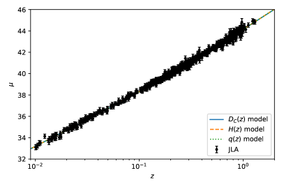
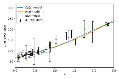
Figure 1: a) SNe Ia distance moduli from JLA. The data for $\mu$ were estimated from Eq. (34), with SNe Ia parameters from the $D_{C}(z)$ model (Table 1) and the error bars comes from the diagonal of the covariance matrix. The lines represent the best fit from SNe+$H(z)$ data for each model. b) 41 $H(z)$ data compilation. The lines represent the best fit from SNe+$H(z)$ data for each model.

II.3 $z_{t}$ from $q(z)$

Now let us see how to assess $z_{t}$ by means of a parametrization of $q(z)$. From (1) one may find $E(z)$

$$E(z)=\exp\left[\int_{0}^{z}\frac{1+q(z^{\prime})}{1+z^{\prime}}dz^{\prime}\right].$$ (28)

If we assume a linear $z$ dependence in $q(z)$, as

$$q(z)=q_{0}+q_{1}z,$$ (29)

which is the simplest $q(z)$ parametrization that allows for a transition, one may find

$$E(z)=e^{q_{1}z}(1+z)^{1+q_{0}-q_{1}},$$ (30)

while the comoving distance $D_{C}(z)$ (6) is given by

$$D_{C}(z)=e^{q_{1}}q_{1}^{q_{0}-q_{1}}\left[\Gamma(q_{1}-q_{0},q_{1})-\Gamma(q_{1}-q_{0},q_{1}(1+z))\right],$$ (31)

where $\Gamma(a,x)$ is the incomplete gamma function defined by AbraSteg as $\Gamma(a,x)\equiv\int_{x}^{\infty}e^{-t}t^{a-1}dt$, with $a>0$.

From (29) (or from (30) and (8)) it is easy to find:

$$z_{t}=-\frac{q_{0}}{q_{1}}\hskip 28.45274pt\textrm{and}\hskip 28.45274ptq_{0}=-q_{1}z_{t},$$ (32)

from which follows $D_{C}(z)$ and $D_{L}(z)$ as a function of just $z_{t}$ and $q_{1}$, which can be constrained from observational data.

III Samples

III.1 $H(z)$ data

Hubble parameter data in terms of redshift yields one of the most straightforward cosmological tests because it is inferred from astrophysical observations alone, not depending on any background cosmological models.

At the present time, the most important methods for obtaining $H(z)$ data are (i) through “cosmic chronometers”, for example, the differential age of galaxies (DAG), (ii) measurements of peaks of acoustic oscillations of baryons (BAO) and (iii) through correlation function of luminous red galaxies (LRG).

The data we work here are a combination of the compilations from Sharov and Vorontsova SharovVor14 and Moresco et al. moresco2016 as described on Jesus et al. JesusHz41 . Sharov and Vorontsova SharovVor14 added 6 $H(z)$ data in comparison to Farooq and Ratra Omer2 compilation, which had 28 measurements. Moresco et al. moresco2016 , on their turn, have added 7 new $H(z)$ measurements in comparison to Sharov and Vorontsova SharovVor14 . By combining both datasets, Jesus et al. JesusHz41 have arrived at 41 $H(z)$ data, as can be seen on Table 1 of JesusHz41 and Figure 1b here.

III.2 JLA SNe Ia compilation

The JLA compilation JLA consists of 740 SNe Ia from the SDSS-II Sako2014 and SNLS C11 collaborations. Actually, this compilation produced recalibrated SNe Ia light-curves and associated distances for the SDSS-II and SNLS samples in order to improve the accuracy of cosmological constraints, limited by systematic measurement uncertainties, as, for instance, the uncertainty in the band-to-band and survey-to-survey relative flux calibration. The light curves have high quality and were obtained by using an improved SALT2 (Spectral Adaptive Light-curve Templates) method JLA ; guy2007 ; guy2010 ; betoule2014 . The data set includes several low-redshift samples ($z<0.1$), all three seasons from the SDSS-II ($0.05\leq z\leq 0.4$) and three years from SNLS ($0.2<z<1.4$). See Fig. 1a and more details in next section.

IV Analyses and Results

In our analyses, we have used flat priors over the parameters, so the posteriors are always proportional to the likelihoods. For $H(z)$ data, the likelihood distribution function is given by $\mathscr{L}_{H}\propto e^{-\frac{\chi^{2}_{H}}{2}}$, where

$$\chi^{2}_{H}=\sum_{i=1}^{41}\frac{{\left[H_{obs,i}-H(z_{i},H_{0},z_{t},\theta_{mod,j})\right]}^{2}}{\sigma^{2}_{H_{i},obs}},$$ (33)

where $\theta_{mod,j}$ is the specific parameter for each model, namely $d_{2}$, $h_{2}$ or $q_{1}$, for $D_{C}(z)$, $H(z)$, $q(z)$ parametrizations, respectively.

As explained on JLA , we may assume that supernovae with identical color, shape and galactic environment have, on average, the same intrinsic luminosity for all redshifts. In this case, the distance modulus $\mu=5\log_{10}(d_{L}(\mathrm{pc})/10)$ may be given by

$$\mu=m_{B}^{*}-(M_{B}-\alpha\times X_{1}+\beta\times C)$$ (34)

where $X_{1}$ describes the time stretching of the light-curve, $C$ describes the supernova color at maximum brightness, $m_{B}^{*}$ corresponds to the observed peak magnitude in the rest-frame $B$ band, $\alpha$, $\beta$ and $M_{B}$ are nuisance parameters. According to C11 , $M_{B}$ may depend on the host stellar mass ($M_{\mathrm{stellar}}$) as

$$M_{B}=\left\{\begin{array}[]{ll}M_{B}^{1}&\mathrm{if}\,\,M_{\mathrm{stellar}}<10^{10}M_{\odot}.\\ M_{B}^{1}+\Delta_{M}&\mathrm{otherwise.}\\ \end{array}\right.$$ (35)

For SNe Ia from JLA, we have the likelihood $\mathscr{L}_{SN}\propto e^{-\frac{\chi^{2}_{SN}}{2}}$, where

$$\chi^{2}_{SN}=\left[\hat{\bm{\mu}}(\theta_{SN})-{\bm{\mu}}(z,z_{t},\theta_{mod,j})\right]^{T}\bm{C}^{-1}\left[\hat{\bm{\mu}}(\theta_{SN})-{\bm{\mu}}(z,z_{t},\theta_{mod,j})\right]$$ (36)

where $\theta_{SN}=(\alpha,\beta,M_{B}^{1},\Delta_{M})$, $\bm{C}$ is the covariance matrix of $\hat{\bm{\mu}}$ as described on JLA , $\bm{\mu}(z,z_{t},\theta_{mod,j})=5\log_{10}(d_{L}(z,z_{t},\theta_{mod,j})/10\,\mathrm{pc})$ computed for a fiducial value $H_{0}=70$ km/s/Mpc.

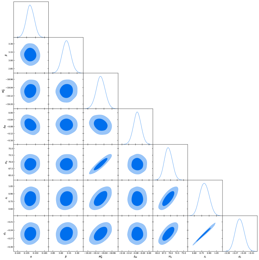
Figure 2: Combined constraints from JLA and $H(z)$ for $D_{C}(z)=z+d_{2}z^{2}+d_{3}z^{3}$.

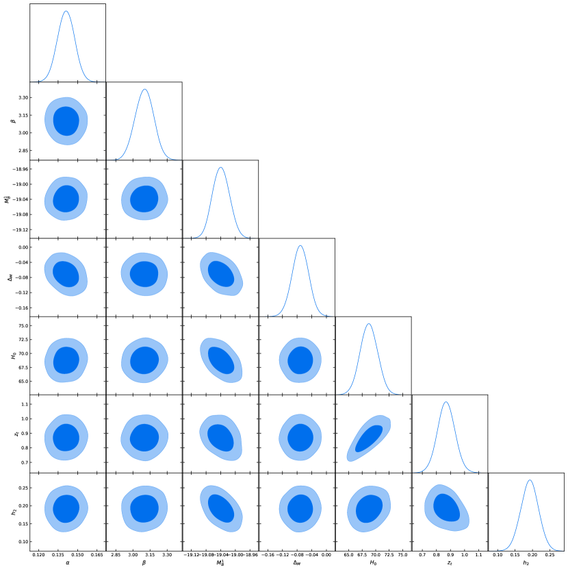
Figure 3: Combined constraints from JLA and $H(z)$ for $H(z)=H_{0}(1+h_{1}z+h_{2}z^{2})$.

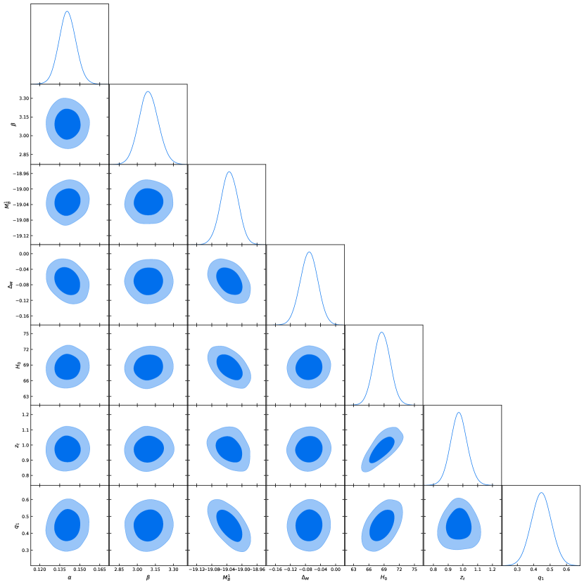
Figure 4: Combined constraints from JLA and $H(z)$ for $q(z)=q_{0}+q_{1}z$.

In order to obtain the constraints over the free parameters, we have sampled the likelihood $\mathscr{L}\propto e^{-\chi^{2}/2}$ through Monte Carlo Markov Chain (MCMC) analysis. A simple and powerful MCMC method is the so-called Affine Invariant MCMC Ensemble Sampler by GoodWeare , which was implemented in Python language with the emcee software by ForemanMackey13 . This MCMC method has advantage over the simple Metropolis-Hastings (MH) method, since it depends only on one scale parameter of the proposed distribution and also on the number of walkers, while MH method is based on the parameter covariance matrix, that is, it depends on $n(n+1)/2$ tuning parameters, where $n$ is the dimension of parameter space. The main idea of the Goodman-Weare affine-invariant sampler is the so called “stretch move”, where the position (parameter vector in parameter space) of a walker (chain) is determined by the position of the other walkers. Foreman-Mackey et al. modified this method, in order to make it suitable for parallelization, by splitting the walkers in two groups, then the position of a walker in one group is determined only by the position of walkers of the other group.

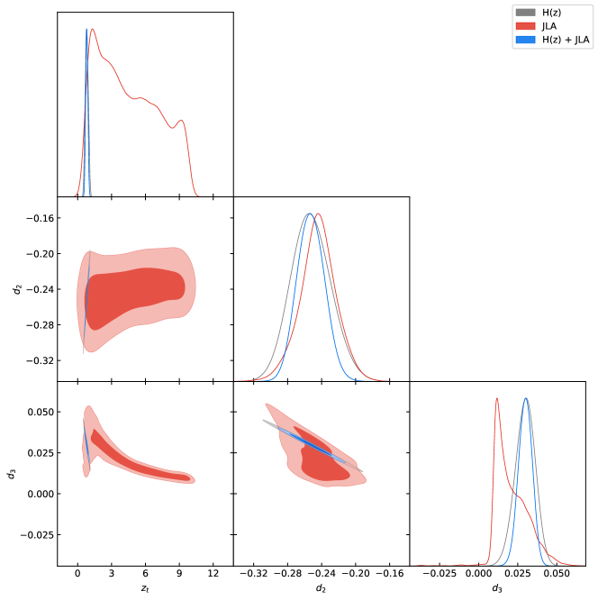
Figure 5: Constraints from JLA and $H(z)$ for $D_{C}(z)=z+d_{2}z^{2}+d_{3}z^{3}$.

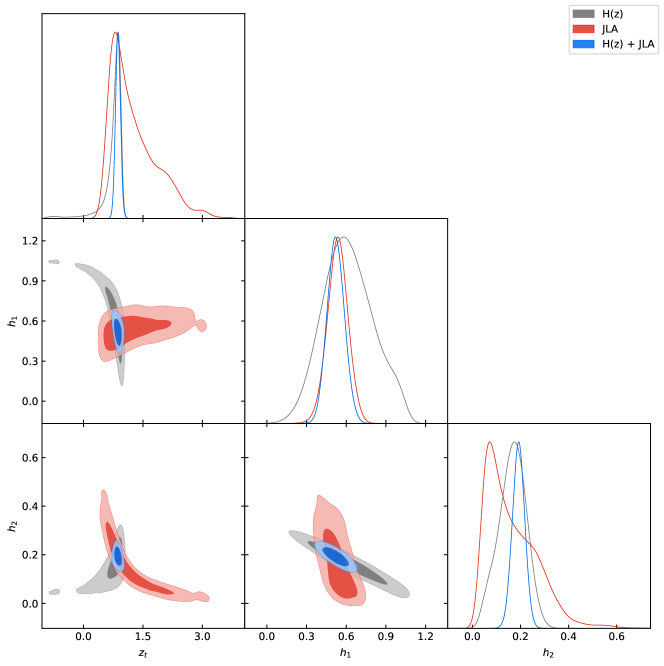
Figure 6: Constraints from JLA and $H(z)$ for $H(z)=H_{0}(1+h_{1}z+h_{2}z^{2})$.

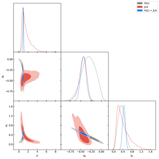
Figure 7: Constraints from JLA and $H(z)$ for $q(z)=q_{0}+q_{1}z$.

We used the freely available software emcee to sample from our likelihood in $n$-dimensional parameter space. We have used flat priors over the parameters. In order to plot all the constraints on each model in the same figure, we have used the freely available software getdist, in its Python version. The results of our statistical analyses can be seen on Figs. 2-8 and on Table 1.

In Figs.2-4, we have the combined results for each parametrization. As one may see, we have always chosen $z_{t}$ as one of our fiducial parameter. The other parameters from each model is later obtained as derived parameters. As one may see in Figs.2-4, the combination of JLA+$H(z)$ yields strong constraints over all parameters, especially $z_{t}$. Also, we find negligible difference in the SNe Ia parameters for each model. We have also to emphasize that the constraints over $H_{0}$ comes just from $H(z)$ while for JLA $H_{0}$ is fixed. We choose not to include other constraints over $H_{0}$ due to the recent tension from different limits over the Hubble constant. At the end of this section, we compare our results with different constraints over $H_{0}$.

In Figs.5-7, we show explicitly the independent constraints from JLA and $H(z)$ over the cosmological parameters. As one may see in Fig.5, SNe Ia sets weaker constraints over $z_{t}$ for $D_{C}(z)$ parametrization. Almost all the $z_{t}$ constraint comes just from $H(z)$. For $d_{2}$, $H(z)$ and JLA yields similar constraints. For $d_{3}$, $H(z)$ yields slightly better constraints. For Figs.6 and 7, the constraints over $z_{t}$ from SNe Ia are improved and one may see how SNe Ia and $H(z)$ complement each other in order to constrain the transition redshift. In Fig. 6, one may see that the constraint over $h_{1}$ is better from JLA. The constraint over $h_{2}$ is better from $H(z)$. In Fig.7, one may see that the constraint over $q_{0}$ is better from JLA. The constraint over $q_{1}$ is better from $H(z)$.

For all parametrizations, the best constraints over the transition redshift comes from $H(z)$ data, as first indicated by limajesus2014 . Moresco et al. moresco2016 also found stringent constraints over $z_{t}$ from $H(z)$ in their parametrization, however, they did not compare with SNe Ia constraints.

Fig.8 summarizes our combined constraints over $z_{t}$ for each parametrization. As one may see, the $q(z)$ model yields the strongest constraints over $z_{t}$. The other parametrizations are important for us to realize how much $z_{t}$ is still allowed to vary. All constraints are compatible at 1$\sigma$ c.l.

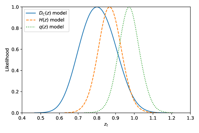
Figure 8: Likelihoods for transition redshift from JLA and $H(z)$ data combined. Blue solid line corresponds to $D_{C}(z)$ parametrization, orange long-dashed line corresponds to $H(z)$ parametrization and green short-dashed line corresponds to $q(z)$ parametrization.

Table 1 shows the full numerical results from our statistical analysis. As one may see the SNe Ia constraints vary little for each parametrization. In fact, we also have found constraints from the (faster) JLA binned data JLA , however, when comparing with the (slower) full JLA constraints, we have found that the full JLA yields stronger constraints over the parameters, especially $z_{t}$. So we decided to deal only with the JLA full data.

Parameter	$D_{C}(z)$	$H(z)$	$q(z)$
$\alpha$	$0.1412\pm 0.0065\pm 0.013$	$0.1412\pm 0.0066\pm 0.013$	$0.1408\pm 0.0064\pm 0.013$
$\beta$	$3.105\pm 0.080\pm 0.16$	$3.101\pm 0.082\pm 0.16$	$3.094\pm 0.080\pm 0.16$
$M_{B}^{1}$	$-19.073\pm 0.044^{+0.089}_{-0.090}$	$-19.039\pm 0.023^{+0.047}_{-0.045}$	$-19.033\pm 0.023^{+0.045}_{-0.046}$
$\Delta_{M}$	$-0.069\pm 0.023\pm 0.046$	$-0.071\pm 0.023^{+0.045}_{-0.046}$	$-0.071\pm 0.023^{+0.046}_{-0.047}$
$H_{0}$	$69.1\pm 1.5\pm 3.0$	$68.8\pm 1.6\pm 3.2$	$68.6\pm 1.6^{+3.3}_{-3.2}$
$z_{t}$	$0.806\pm 0.094^{+0.19}_{-0.18}$	$0.870\pm 0.063^{+0.13}_{-0.12}$	$0.973\pm 0.058^{+0.12}_{-0.11}$
$d_{2}$	$-0.253\pm 0.016^{+0.033}_{-0.031}$	–	–
$d_{3}$	$0.0299\pm 0.0044^{+0.0085}_{-0.0090}$	–	–
$h_{1}$	–	$0.522\pm 0.065\pm 0.13$	–
$h_{2}$	–	$0.192\pm 0.026^{+0.051}_{-0.052}$	–
$q_{0}$	–	–	$-0.434\pm 0.065\pm 0.13$
$q_{1}$	–	–	$0.446\pm 0.062\pm 0.12$

Table 1: Constraints from JLA+$H(z)$ for $D_{C}(z)$, $H(z)$ and $q(z)$ parametrizations. The parameters without bold faces were treated as derived parameters. The central values correspond to the mean and the 1 $\sigma$ and 2 $\sigma$ c.l. correspond to the minimal 68.3% and 95.4% confidence intervals.

By using 30 $H(z)$ data, plus $H_{0}$ from Riess et al. (2011) Riess11 , Moresco et al. moresco2016 found $z_{t}=0.64^{+0.1}_{-0.06}$ for $\Lambda$CDM and $z_{t}=0.4\pm 0.1$ for their model independent approach. Only our $D_{C}(z)$ parametrization is compatible with their model-independent result. Their $\Lambda$CDM result is compatible with all our parametrizations, although it is marginally compatible with $q(z)$.

Another interesting result that can be seen in Table 1 is the $H_{0}$ constraint. As one may see, the constraints over $H_{0}$ are consistent through the three different parametrizations, with a little smaller uncertainty for $D_{C}(z)$, $H_{0}=69.1\pm 1.5$ km/s/Mpc. The constraints over $H_{0}$ are quite stringent today from many observations RiessEtAl16 ; Planck16 . However, there is some tension among $H_{0}$ values estimated from Cepheids RiessEtAl16 and from CMB Planck16 . While Riess et al. advocate $H_{0}=73.24\pm 1.74$ km/s/Mpc, the Planck collaboration analysis yields $H_{0}=66.93\pm 0.62$ km/s/Mpc, a 3.4$\sigma$ lower value. It is interesting to note, from our Table 1 that, although we are working with model independent parametrizations and data at intermediate redshifts, our result is in better agreement with the high redshift result from Planck. In fact, all our results are compatible within 1$\sigma$ with the Planck’s result, while it is incompatible at 3$\sigma$ with the Riess’ result.

V Conclusion

The accelerated expansion of Universe is confirmed by different sets of cosmological observations. Several models proposed in literature satisfactorily explain the transition from decelerated phase to the current accelerated phase. A more significant question is when the transition occurs from one phase to another, and the parameter that measures this transition is called the transition redshift, $z_{t}$. The determination of $z_{t}$ is strongly dependent on the cosmological model adopted, thus the search for methods that allow the determination of such parameter in a model independent way are of fundamental importance, since it would serve as a test for several cosmological models.

In the present work, we wrote the comoving distance $D_{C}$, the Hubble parameter $H(z)$ and the deceleration parameter $q(z)$ as third, second and first degree polynomials on $z$, respectively (see equations (9), (17) and (29)), and obtained, for each case, the $z_{t}$ value. Only a flat universe was assumed and the estimates for $z_{t}$ were obtained, independent of a specific cosmological model. As observational data, we have used Supernovae type Ia and Hubble parameter measurements. Our results can be found in Figures 2-7. As one may see from Figs. 5-7, the analyses by using SNe Ia (red color) and $H(z)$ data (blue color) are complementary to each other, providing tight limits in the parameter spaces. As a result, the values obtained for the transition redshift in each case were $0.806\pm 0.094$, $0.870\pm 0.063$ and $0.973\pm 0.058$ at 1$\sigma$ c.l., respectively (see Fig. 8).

- (1) A. G. Riess et al. [Supernova Search Team], Astron. J. 116 (1998) 1009 [astro-ph/9805201].
- (2) S. Perlmutter et al. [Supernova Cosmology Project Collaboration], Astrophys. J. 517 (1999) 565 [astro-ph/9812133].
- (3) P. Astier et al. [SNLS Collaboration], Astron. Astrophys. 447 (2006) 31 [astro-ph/0510447].
- (4) A. G. Riess et al., Astrophys. J. 659 (2007) 98 [astro-ph/0611572].
- (5) T. M. Davis et al., Astrophys. J. 666 (2007) 716 [astro-ph/0701510].
- (6) M. Kowalski et al. [Supernova Cosmology Project Collaboration], Astrophys. J. 686 (2008) 749 [arXiv:0804.4142 [astro-ph]].
- (7) R. Amanullah et al., Astrophys. J. 716 (2010) 712 [arXiv:1004.1711 [astro-ph.CO]].
- (8) N. Suzuki et al., Astrophys. J. 746 (2012) 85 [arXiv:1105.3470 [astro-ph.CO]].
- (9) E. Komatsu et al. [WMAP Collaboration], Astrophys. J. Suppl. 192 (2011) 18 [arXiv:1001.4538 [astro-ph.CO]].
- (10) D. Larson et al., Astrophys. J. Suppl. 192 (2011) 16 [arXiv:1001.4635 [astro-ph.CO]].
- (11) P. A. R. Ade et al. [Planck Collaboration], Astron. Astrophys. 571 (2014) A16 [arXiv:1303.5076 [astro-ph.CO]].
- (12) D. J. Eisenstein et al. [SDSS Collaboration], Astrophys. J. 633 (2005) 560 [astro-ph/0501171].
- (13) W. J. Percival, S. Cole, D. J. Eisenstein, R. C. Nichol, J. A. Peacock, A. C. Pope and A. S. Szalay, Mon. Not. Roy. Astron. Soc. 381 (2007) 1053 [arXiv:0705.3323 [astro-ph]].
- (14) D. Schlegel et al. [with input from the SDSS-III Collaboration], arXiv:0902.4680 [astro-ph.CO].
- (15) D. J. Eisenstein et al. [SDSS Collaboration], Astron. J. 142 (2011) 72 [arXiv:1101.1529 [astro-ph.IM]].
- (16) K. S. Dawson et al. [BOSS Collaboration], Astron. J. 145 (2013) 10 [arXiv:1208.0022 [astro-ph.CO]].
- (17) O. Farooq, D. Mania and B. Ratra, Astrophys. J. 764 (2013) 138 [arXiv:1211.4253 [astro-ph.CO]].
- (18) O. Farooq and B. Ratra, Astrophys. J. 766 (2013) L7 [arXiv:1301.5243 [astro-ph.CO]].
- (19) O. Farooq, F. R. Madiyar, S. Crandall and B. Ratra, Astrophys. J. 835 (2017) no.1, 26 [arXiv:1607.03537 [astro-ph.CO]].
- (20) S. Weinberg, Rev. Mod. Phys. 61 (1989) 1.
- (21) T. Padmanabhan, Phys. Rept. 380 (2003) 235 [hep-th/0212290].
- (22) M. Davis, G. Efstathiou, C. S. Frenk and S. D. M. White, Astrophys. J. 292 (1985) 371.
- (23) G. Bertone, Particle Dark Matter: Observations, Models and Searches, Cambridge University Press, UK, (2010).
- (24) D. H. Weinberg, M. J. Mortonson, D. J. Eisenstein, C. Hirata, A. G. Riess and E. Rozo, Phys. Rept. 530 (2013) 87 doi:10.1016/j.physrep.2013.05.001 [arXiv:1201.2434 [astro-ph.CO]].
- (25) G. S. Sharov and E. G. Vorontsova, JCAP 1410 (2014) no.10, 057 [arXiv:1407.5405 [gr-qc]].
- (26) P. J. E. Peebles and B. Ratra, Rev. Mod. Phys. 75 (2003) 559 [astro-ph/0207347].
- (27) V. Sahni and A. Starobinsky, Int. J. Mod. Phys. D 15 (2006) 2105 [astro-ph/0610026].
- (28) M. S. Volkov, Phys. Rev. D 86, (2012) 061502;
- (29) M. Milgrom, Astrophys. J. 270, (1983) 365; Astrophys. J. 270 (1983) 371;
- (30) G. Gentile, B. Famaey, W.J.G. de Blok, Astron. Astrophys. 527 (2011) A76.
- (31) T. P. Sotiriou and V. Faraoni, Rev. Mod. Phys. 82 (2010) 451;
- (32) J. Q. Guo and A.V. Frolov, Phys. Rev. D 88 (2013) 124036;
- (33) S. Capozziello and M. De Laurentis, Phys. Rep. 509 (2011) 167.
- (34) L. Randall and R. Sundrum, Phys. Rev. Lett. 83, (1999) 4690; [arXiv:hep-th/9906064].
- (35) A. Falkowski, Z. Lalak and S. Pokorski, Phys. Lett. B 491, (2000) 172; [arXiv:hep-th/0004093];
- (36) P. Binetruy, C. Deffayet and D. Langlois, Nucl. Phys. B 565 (2000) 269; [arXiv:hep-th/9905012];
- (37) T. Shiromizu, K. I. Maeda and M. Sasaki, Phys. Rev. D 62 (2000) 024012; [arXiv:gr-qc/9910076].
- (38) J. M. Cline, C. Grojean and G. Servant, Phys. Rev. Lett. 83 (1999) 4245; [arXiv:hep-ph/9906523].
- (39) T. Damour and A. M. Polyakov, Gen.Rel.Grav. 26 (1994) 1171; [gr-qc/9411069].
- (40) J. M. Overduin and P. S. Wesson, Phys. Rept. 283 (1997) 303; [gr-qc/9805018].
- (41) M. Visser, Class. Quant. Grav. 21 (2004) 2603 [gr-qc/0309109].
- (42) M. Visser, Gen. Rel. Grav. 37 (2005) 1541 [gr-qc/0411131].
- (43) C. Shapiro and M. S. Turner, Astrophys. J. 649 (2006) 563 [astro-ph/0512586].
- (44) R. D. Blandford, M. A. Amin, E. A. Baltz, K. Mandel and P. J. Marshall, ASP Conf. Ser. 339 (2005) 27 [astro-ph/0408279].
- (45) Ø. Elgarøy and T. Multamäki, JCAP 0609 (2006) 002 [astro-ph/0603053].
- (46) D. Rapetti, S. W. Allen, M. A. Amin and R. D. Blandford, Mon. Not. Roy. Astron. Soc. 375 (2007) 1510 [astro-ph/0605683].
- (47) J. V. Cunha and J. A. S. Lima, Mon. Not. Roy. Astron. Soc. 390 (2008) 210 [arXiv:0805.1261 [astro-ph]].
- (48) A. C. C. Guimaraes, J. V. Cunha and J. A. S. Lima, JCAP 0910 (2009) 010 [arXiv:0904.3550 [astro-ph.CO]].
- (49) N. Rani, D. Jain, S. Mahajan, A. Mukherjee and N. Pires, JCAP 1512 (2015) no.12, 045 [arXiv:1503.08543 [gr-qc]].
- (50) L. Xu, W. Li and J. Lu, JCAP 0907 (2009) 031 [arXiv:0905.4552 [astro-ph.CO]].
- (51) R. F. L. Holanda, J. S. Alcaniz and J. C. Carvalho, JCAP 1306 (2013) 033 [arXiv:1303.3307 [astro-ph.CO]].
- (52) A. Sandage, Physics Today, February 23, 34 (1970).
- (53) J. A. S. Lima, J. F. Jesus, R. C. Santos and M. S. S. Gill, arXiv:1205.4688 [astro-ph.CO].
- (54) M. Moresco et al., JCAP 1605 (2016) no.05, 014 [arXiv:1601.01701 [astro-ph.CO]].
- (55) M. Betoule et al. [SDSS Collaboration], Astron. Astrophys. 568 (2014) A22 [arXiv:1401.4064 [astro-ph.CO]].
- (56) M. Abramowitz, & I. A. Stegun, Handbook of mathematical functions: with formulas, graphs, and mathematical tables, Vol. 55, (1964) Courier Corporation.
- (57) G. S. Sharov, and E. G. Vorontsova, JCAP 1410 (2014) no.10, 057 [arXiv:1407.5405 [gr-qc]].
- (58) J. F. Jesus, T. M. Gregório, F. Andrade-Oliveira, R. Valentim and C. A. O. Matos, Mon. Not. Roy. Astron. Soc. 477 (2018) 2867 [arXiv:1709.00646 [astro-ph.CO]].
- (59) M. Sako et al. [SDSS Collaboration], arXiv:1401.3317 [astro-ph.CO].
- (60) A. Conley et al. [SNLS Collaboration], Astrophys. J. Suppl. 192 (2011) 1 [arXiv:1104.1443 [astro-ph.CO]].
- (61) J. Guy, P. Astier, S. Baumont, D. Hardin, R. Pain et al., 2007, A&A, 466, 11–21.
- (62) J. Guy, M.Sullivan, A. Conley, N. Regnault, P.Astier, C. Balland et al. 2010, A&A, 523, A7.
- (63) M. Betoule, R Kessler, J Guy, J Mosher, D Hardin, et al., (2014), A&A, 568, A22.
- (64) J. Goodman, and J. Weare, Comm. App. Math. Comp. Sci., (2010) v.5, 1, 65
- (65) D. Foreman-Mackey, D. W. Hogg, D. Lang and J. Goodman, Publ. Astron. Soc. Pac. 125 (2013) 306 [arXiv:1202.3665 [astro-ph.IM]].
- (66) R. Allison, and J. Dunkley, Mon. Not. Roy. Astron. Soc. 437, (2014), no.4, 3918 [arXiv:1308.2675 [astro-ph.IM]].
- (67) A. Lewis, and S. Bridle, Phys. Rev. D 66, (2002) 103511 [astro-ph/0205436].
- (68) A. G. Riess, et al., Astrophys. J. 730 (2011) 119 Erratum: [Astrophys. J. 732 (2011) 129] [arXiv:1103.2976 [astro-ph.CO]].
- (69) Riess, A.G. et al., Astrophys. J. 826 (2016) no.1, 56 [arXiv:1604.01424 [astro-ph.CO]].
- (70) Ade, P.A.R. et al. [Planck Collaboration], Astron. Astrophys. 594 (2016) A13 [arXiv:1502.01589 [astro-ph.CO]].
- (71) Bernal, J.L., Verde, L. and Riess, A.G., JCAP 1610 (2016) no.10, 019 [arXiv:1607.05617 [astro-ph.CO]].