Chemical fingerprints of hot Jupiter planet formation

Abstract

Context. The current paradigm to explain the presence of Jupiter-like planets with small orbital periods (P $<$ 10 days; hot Jupiters), which involves their formation beyond the snow line following inward migration, has been challenged by recent works that explore the possibility of in situ formation.

Aims. We aim to test whether stars harbouring hot Jupiters and stars with more distant gas-giant planets show any chemical peculiarity that could be related to different formation processes.

Methods. Our methodology is based on the analysis of high-resolution échelle spectra. Stellar parameters and abundances of C, O, Na, Mg, Al, Si, S, Ca, Sc, Ti, V, Cr, Mn, Co, Ni, Cu, and Zn for a sample of 88 planet hosts are derived. The sample is divided into stars hosting hot (a $<$ 0.1 au) and cool (a $>$ 0.1 au) Jupiter-like planets. The metallicity and abundance trends of the two sub-samples are compared and set in the context of current models of planet formation and migration.

Results. Our results show that stars with hot Jupiters have higher metallicities than stars with cool distant gas-giant planets in the metallicity range +0.00/+0.20 dex. The data also shows a tendency of stars with cool Jupiters to show larger abundances of $\alpha$ elements. No abundance differences between stars with cool and hot Jupiters are found when considering iron peak, volatile elements or the C/O, and Mg/Si ratios. The corresponding $p$-values from the statistical tests comparing the cumulative distributions of cool and hot planet hosts are 0.20, $<$ 0.01, 0.81, and 0.16 for metallicity, $\alpha$, iron-peak, and volatile elements, respectively. We confirm previous works suggesting that more distant planets show higher planetary masses as well as larger eccentricities. We note differences in age and spectral type between the hot and cool planet host samples that might affect the abundance comparison.

Conclusions. The differences in the distribution of planetary mass, period, eccentricity, and stellar host metallicity suggest a different formation mechanism for hot and cool Jupiters. The slightly larger $\alpha$ abundances found in stars harbouring cool Jupiters might compensate their lower metallicities allowing the formation of gas-giant planets.

1 Introduction

The discovery of gas-giant planets orbiting their parent stars at close distances, the so-called hot Jupiters (e.g. Mayor & Queloz, 1995; Butler et al., 1997), was an unexpected surprise, as no planets like these are present in our own solar system. It was noticed early on that the gas temperature in the inner region of the protoplanetary disc was too high to allow for the condensation of solid particles and also that the available mass so close to the star was not enough to form a Jupiter mass object (Boss, 1995; Bodenheimer et al., 2000; Rafikov, 2006). Therefore, it was proposed that all Jupiter-size planets form at relatively low temperatures beyond the snowline and that hot Jupiters experience subsequent inward migration to their current locations (Lin et al., 1996). Currently, migration mechanisms are divided into two main categories: models that involve disc migration (e.g. Goldreich & Tremaine, 1980; Pollack et al., 1996; Ward, 1997; Papaloizou & Larwood, 2000; Alibert et al., 2005; Ida & Lin, 2008; Mordasini et al., 2009; Bromley & Kenyon, 2011; Kley & Nelson, 2012), and models that involve secular high planet eccentricity that need a mechanism to drive it, involving either planet-planet encounters (e.g. Rasio & Ford, 1996; Ford & Rasio, 2006, 2008; Chatterjee et al., 2008; Jurić & Tremaine, 2008; Matsumura et al., 2010; Nagasawa & Ida, 2011; Beaugé & Nesvorný, 2012; Boley et al., 2012), secular Lidov-Kozai (LK) oscillations (Lidov, 1962; Kozai, 1962) induced by a companion (e.g. Wu & Murray, 2003; Fabrycky & Tremaine, 2007; Naoz et al., 2012), or secular chaos (Wu & Lithwick, 2011; Hamers et al., 2016).

The formation of gas-giant planets at wide stellar separations by core-accretion faces the obstacle of an excessively long timescale (e.g. Dodson-Robinson et al., 2009; Rafikov, 2011). The so-called pebble accretion mechanism (in which small particles with sizes ranging from millimetres to centimetres constitute the main drivers of planetary growth) has been shown to accelerate the growth speed of planetary cores (Johansen & Lacerda, 2010; Ormel & Klahr, 2010; Lambrechts & Johansen, 2012, 2014; Johansen & Lambrechts, 2017). Population synthesis models based on pebble accretion strongly suggest that snowlines are the preferred places for planet formation (Ali-Dib et al., 2017).

However, recently, several works have addressed the question of whether the in situ formation through core accretion of hot Jupiters might be possible (Batygin et al., 2016; Boley et al., 2016). The reason is twofold. Firstly, the lack of enough material in the innermost region of the protoplanetary nebula is mainly based on models of the solar nebula and it is possible that the solar nebula is not representative of the general conditions of disc forming planets (e.g. Chiang & Laughlin, 2013). In particular, small planets (mini-Neptunes or Super-Earths) not present in the solar system, have been found to be quite common in multiple systems at small orbital periods (Mayor et al., 2011; Cassan et al., 2012; Howard et al., 2012; Fressin et al., 2013; Petigura et al., 2013). Although stating the obvious, it is important to recall that irrespective of whether or not the innermost parts of the disks are suitable for planet formation it is expected that in the colder parts of the disk, solid condensation should be important.

Secondly, evidence has accumulated over recent years that hot Jupiters and more distant gas-giant planets have different properties. To start with, their frequencies are different. It has been shown that even after accounting for possible observational biases (Knutson et al., 2014; Bryan et al., 2016), there are two distinct peaks in the orbital period distribution of Jupiter-class planets: one for hot Jupiters (representing 0.5-1.0% of Sun-type stars (Wright et al., 2012)) at orbital periods close to three days and the average giant planet population that shows periods of 100 days $<$ $P$ $<$ 3000 days (representing 10.5% of the nearby FGK stars (Cumming et al., 2008)). Between these distances the planetary distribution shows a clear dip or “valley” (e.g. Jones et al., 2003; Wright et al., 2009; Currie, 2009). In a recent work, Santerne et al. (2016) analysed a sample of 129 giant planets with periods less than 400 days taken from the Kepler catalogue of transit candidates. The authors find a frequency of hot Jupiters around FGK stars in the Kepler data in the range 0.4-0.5% while the occurrence rate from radial velocity surveys is of the order of $\sim$ 1%. Such a difference might be related to the gas-giant planet-metallicity correlation as the Kepler sample is found to differ in metallicity by about 0.15-0.20 dex from the solar neighbourhood. A similar discrepancy is also found for giant planets in the period valley, with frequencies of 0.90% (Santerne et al., 2016), and $\sim$ 1.6% (Fressin et al., 2013; Mayor et al., 2011). For planets with periods longer than $\sim$ 85 days, the occurrence estimates from the different surveys are compatible with an occurrence rate of $\sim$ 3%.

Hot Jupiters show masses below that of, or of the order of, Jupiter. On the other hand, cool distant gas-giant planets have masses of several times Jupiter’s mass (e.g., Batygin et al., 2016). Furthermore, a tendency for the eccentricities to increase with the planet mass has also been noticed (see Ribas & Miralda-Escudé, 2007, and references therein). The occurrence of additional long-period planets in stars with hot Jupiters is still debated. Schlaufman & Winn (2016) found no difference in the companion fraction between hot and cool Jupiters, either inside or outside the water-ice line, a result that is inconsistent with the simplest models of high-eccentricity migration. Concurrently, Dong et al. (2017) using data from the Kepler mission show that hot Jupiters as well as hot Neptunes are preferentially found in systems with one transiting planet, in agreement with previous works also based on Kepler data (Latham et al., 2011; Steffen et al., 2012; Huang et al., 2016). These results, however, should be regarded with caution as it has been argued that transit detection might be biased towards short-period planets (e.g. Schlaufman & Winn, 2016).

Regarding the metallicity abundance of planet hosts, although no clear correlations between the stellar metallicity and the planetary semimajor axis were found (Udry & Santos, 2007; Valenti & Fischer, 2008; Ammler-von Eiff et al., 2009), several authors have noted a tendency of stars with hot Jupiters planets to show slightly larger metallicities than stars with more distant planets (Sozzetti, 2004), especially in the “low”-metallicity range (between -0.50 dex and + 0.00 dex; (Maldonado et al., 2015)). Furthermore, Maldonado et al. (2015) note that there are no hot Jupiters harbouring stars with significant low metallicities (below -0.50/-0.60 dex), while some cool Jupiters can be found around stars as metal-poor as -1.00 dex. Several works have suggested that the architecture of a planet (period and eccentricity) might indeed show a dependence on the host star’s metallicity (Ribas & Miralda-Escudé, 2007; Dawson & Murray-Clay, 2013; Beaugé & Nesvorný, 2013; Adibekyan et al., 2013). More recently, Bashi et al. (2017) and Santos et al. (2017) suggest that stars hosting massive gas-giant planets show on average lower metallicities than the stars hosting planets with masses below $\sim$ 4-5 M_Jup. A possible correlation between planetary mass and stellar metallicity have been also suggested by Jenkins et al. (2017).

We believe that our current knowledge on hot-Jupiter formation mechanisms would benefit from a detailed chemical abundance analysis of a large sample of stars harbouring hot and cool gas-giant planets, including a large number of ions besides iron. Therefore, in this paper we present a homogeneous analysis of a large sample of stars hosting gas-giant planets that is based on high-resolution and high signal-to-noise ratio échelle spectra.

This paper is organised as follows. Section 2 describes the stellar sample, the observations, and the spectroscopic analysis. The comparison of the abundances of stars with hot and cool Jupiters is presented in Sect. 3 where a search for correlations between the stellar abundances and the planetary properties is also presented. The results are set in the context of current planet formation models in Sect. 4. Our conclusions follow in Sect. 5.

2 Data and spectroscopic analysis

2.1 Stellar sample and observations

Two samples of main sequence (MS) stars, one of cool gas-giant planet hosts (hereafter cool PHs, semimajor axis a $>$ 0.1 au), and another one of stars harbouring hot gas-giant planets (hot PHs, semimajor axis a $<$ 0.1 au), were built by carefully checking the data available at the Extrasolar Planets Encyclopaedia (Schneider et al., 2011). Only radial velocity planets were considered for this work as transit targets are known to have systematically lower metallicities than radial velocity targets (Gould et al., 2006; Howard et al., 2012; Wright et al., 2012; Dawson & Murray-Clay, 2013) and there is no bias that prevents RV detection at small orbital periods. The division at a = 0.1 au comes from the known distribution of planetary semimajor axis where an enhanced frequency of close-in gas-giant planets is found at semimajor axes $\leq$ 0.07 au (e.g. Wright et al., 2009; Currie, 2009). Stars with multiple planets are classified as hot PHs if at least one of the planets has a semimajor axis lower than 0.1 au. We note, however, that the pileup of planets at $\sim$ 3 days is present when the full data set of known planets (dominated by transit surveys) is considered, while it is not obvious when only radial velocity or Kepler data is analysed (Boley et al., 2016).

For this work, all planetary hosts with spectral types between F5 and K2 and available values of planetary mass (M_p$\sin i$), and semimajor axis were considered. Stars with low-mass planets (M_p$\sin i$ $<$ 30M_⊕) are not included since these stars have been the focus of exhaustive analysis and do not present metallicity signatures similar to the ones found for stars hosting gas-giant planets (Ghezzi et al., 2010b; Mayor et al., 2011; Sousa et al., 2011; Buchhave et al., 2012; Buchhave & Latham, 2015). Objects with masses (M_p$\sin i$ $>$ 13M_Jup) have also not been included in this analysis since their masses enter into the brown dwarf domain, their formation mechanism might be different altogether from planets, and the analysis of their abundances have been the subject of a separate study (Maldonado & Villaver, 2017). Whether or not giant stars with planets follow the gas-giant planet metallicity correlation seen in MS planet hosts has been the subject of recent discussions (Sadakane et al., 2005; Schuler et al., 2005; Hekker & Meléndez, 2007; Pasquini et al., 2007; Takeda et al., 2008; Ghezzi et al., 2010a; Maldonado et al., 2013; Mortier et al., 2013; Jofré et al., 2015; Reffert et al., 2015; Maldonado & Villaver, 2016). We therefore excluded all stars with $\log g$ values (see following Section) lower than 4.0 (cgs).

The high-resolution spectra used in this work were collected from public archives. FEROS (Kaufer et al., 1999) data from the ESO archive were taken for 74 stars, while for 8 stars HARPS spectra were used (Mayor et al., 2003). Additional data for 5 stars was taken from the SOPHIE (Bouchy & Sophie Team, 2006) archive while for the star HIP 7513 ($\upsilon$ And) a spectrum taken with the 2dcoudé spectrograph at the McDonald Observatory (Tull et al., 1995) from the public library “S⁴N” (Allende Prieto et al., 2004) was analysed. All spectra were reduced by the corresponding pipelines which implement the typical corrections involved in échelle spectra reduction. The spectra were corrected for radial velocity shifts by using radial velocity standard stars or the radial velocities provided by the reduction pipelines. Typical values of the signal-to-noise ratio are between 80 and 230 (measured in the region around 605 nm). The properties of the different spectra are summarised in Table 1.

Table 1: Properties of the different spectrographs used in this work.

Spectrograph	Spectral range (Å)	Resolving power	$N$ stars
FEROS	3500-9200	48000	74
HARPS	3780-6910	115000	8
SOPHIE	3872-6943	75000	5
2dcoudé	3400-10000	60000	1

The total number of stars in the cool-PHs amounts to 59: 4 F-type stars, 44 G-type stars, and 11 K-type stars. Hot-PHs account for 29 stars: 7 F-type stars, 13 G-type stars, and 9 K-type stars. The stars are listed in Table LABEL:parameters_table_full. All the planetary data used in this work – minimum mass, semimajor axis, planetary period, and eccentricity (Sect. 3) – come from the Extrasolar Planets Encyclopaedia (Schneider et al., 2011).

2.2 Spectroscopic analysis

Basic stellar parameters T_eff, $\log g$, microturbulent velocity $\xi_{\rm t}$, and [Fe/H] are determined using the code TGVIT (Takeda et al., 2005), which implements the iron ionisation and excitation balance, a methodology widely applied to solar-like stars. The line list as well as the adopted parameters (excitation potential, $\log(gf)$ values) can be found on Y. Takeda’s web page . This code makes use of ATLAS9, plane-parallel, LTE atmosphere models (Kurucz, 1993).

TGVIT derives the uncertainties in the stellar parameters by progressively changing each stellar parameter from the converged solution to a value in which the excitation equilibrium, the match of the curve of grow, or the ionisation equilibrium condition are no longer fulfilled (Takeda et al., 2002).

Stellar evolutionary parameters, age, mass, and radius, were computed from Hipparcos V magnitudes (ESA, 1997) and parallaxes (van Leeuwen, 2007) using the code PARAM (da Silva et al., 2006), which is based on the use of Bayesian methods, together with the PARSEC set of isochrones (Bressan et al., 2012). These parameters are provided in Table LABEL:parameters_table_full.

Chemical abundance of individual elements C, O, Na, Mg, Al, Si, S, Ca, Sc, Ti, V, Cr, Mn, Co, Ni, Cu, and Zn was obtained using the 2014 version of the code MOOG (Sneden, 1973) together with ATLAS9 atmosphere models (Kurucz, 1993). The measured equivalent widths (EWs) of a list of narrow, non-blended lines for each of the aforementioned species are used as inputs. The selected lines are taken from the list provided by Maldonado et al. (2015). Hyperfine structure (HFS) was taken into account for V i, Co i, and Cu i abundances. Oxygen abundances derived from O i triplet lines at 777 nm are known to be severely affected by departures from LTE (e.g. Kiselman, 1993, 2001). To account for non-LTE effects, the prescriptions given by Takeda (2003) were followed.

Our derived abundances are provided in Table LABEL:abundance_table_full. They are expressed relative to the solar values derived in Maldonado et al. (2015). Errors take into account the line-to-line scatter as well as the propagation of the uncertainties of the stellar parameters in the abundances following the results by Maldonado et al. (2015).

Given the difficulties of obtaining reliable abundances of some volatile elements, in particular C i and O i , we compared our derived C and O ratios (C/Os) with the works of Teske et al. (2014) and Schuler et al. (2015). Since a star-to-star comparison is not possible, as no stars in common are available, we compare the corresponding cumulative distribution function; Figure 1. We restrict the comparison to stars with C/Os lower than one (to use the same range of values than the literature samples). We also discard for the analysis those stars with high uncertainties in the derived C/O values. The comparison reveals a tendency of slightly larger values in our sample. A Kolmogorv-Smirnov test (hereafter K-S test) returns a K-S statistics of 0.34, and a $p$-value of 0.03 (n_eff = 16.5).

We do not know the reason for this discrepancy. While it might be related to some difference in the methodology to derive abundances (e.g. line selection, atomic data), it could also be an effect of the different samples considered in this work. We note that the samples in Teske et al. (2014) and Schuler et al. (2015) consist in stars with transiting planets, while this work is focused on radial velocity planets.

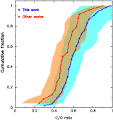
Figure 1: Comparison between the C/Os derived in this work and those from Teske et al. (2014) and Schuler et al. (2015).

2.3 Kinematics

Galactic spatial velocity components $(U,V,W)$ are computed following the procedure described in Montes et al. (2001). Parallaxes were taken from the revised reduction of the Hipparcos data (van Leeuwen, 2007) while proper motions are from the Tycho-2 catalogue (Høg et al., 2000). Radial velocities are mainly from the compilation by Malaroda et al. (2006). Finally, stars were classified as belonging to the thin/thick disk applying the methodology described in Bensby et al. (2003, 2005). This classification is provided in Table LABEL:parameters_table_full.

2.4 Properties of the stellar samples

It is well known that some stellar properties, such as distance, age, or kinematics, can affect the metal content of a star. Therefore before a comparison of metallicity and abundances of hot and cool PHs is made, an analysis of the stellar properties of both samples is mandatory. This analysis is presented in Table 2 where both samples are compared by using a K-S test. In order to account for the uncertainties in the stellar parameters a series of 10⁶ simulations were performed. In each simulation the property of each star is randomly varied within its corresponding uncertainty. For each series of simulated data a K-S test is performed. Assuming that the distribution of the simulated $p$-values follows a Gaussian function we then compute the probability that the simulated $p$-value takes the value (within 5%) found when analysing the original data.

According to the KS test, both samples are quite similar in terms of stellar distance. The analysis reveals a tendency of hot PHs to be slightly fainter and younger than the cool PHs. This effect can also be seen in Figure 2 where the corresponding cumulative distribution functions of the V magnitude (upper left panel) and the stellar age (upper right panel) are shown. The hatched regions indicate the limits of the cumulative distributions built by considering that all stars have a stellar parameter $P$ equal to $P$ + $\Delta P$ and $P$ - $\Delta P$. We note that although the uncertainties in the stellar age are large, the derived $p$-value is highly significant (the probability of being due to the uncertainties is only 3%). We also note a slightly larger fraction of F-type stars in the hot-PH sample. As we do not have any explanation for that we will explore this potential bias in more detail in Sect. 4.1.

Regarding kinematics, the kinematic criteria for thick/thin disc membership does not reveal any significant difference between hot and cool PHs as most of the stars in both samples appear to belong to the thin disc population. Figure 3 shows the corresponding Toomre diagram where it can be seen that both hot- and cool-PHs are well mixed in the vertical axis. However, the range of $V_{\rm LSR}$ values of the hot PHs is narrower than that of the cool PHs, and therefore a tendency of hot PHs to show larger $V_{\rm LSR}$ values in the corresponding cumulative distribution function at low values (between -10 and -50 km s^-1) is found (Fig. 2, bottom left). In addition, a comparison in terms of mean Galactocentric distance, R_mean, was performed as the Galactic birth place has been suggested to be related to the chemical properties of planet hosts (Adibekyan et al., 2014, 2016). Values of R_mean are taken from Casagrande et al. (2011). While the K-S test reveals no significant differences between hot and cool PHs, the plot of the corresponding cumulative distributions (Fig. 2, bottom right) shows a tendency of hot PHs to be located at slightly larger R_mean values in the R_mean range 6.5-7.8 Kpc.

Other properties such as stellar mass or effective temperature were analysed but no differences between the two samples were found.

Table 2: Comparison between the properties of cool and hot PHs.

	cool PHs			hot PHs			K-S test
	Mean	Median	Range	Mean	Median	Range	$D$	$p$-value	$p$-sig.
V (mag)	7.3	7.5	3.7/9.6	7.6	8.0	4.1/10	0.32	0.03	0.31
Distance (pc)	41.6	38.11	3.2/103	43.9	42.7	12.5/95	0.16	0.64	0.13
Age (Gyr)	4.2	3.9	0.31/11.4	3.0	2.4	0.1/11	0.28	0.09	0.03
Mass (M⊙)	1.07	1.08	0.77/1.41	1.08	1.07	0.83/1.41	0.09	0.99	0.20
Teff	5723	5761	4849/6472	5741	5656	5025/6704	0.19	0.41	0.13
$V_{\rm LSR}$ (km s-1)	-10.23	-7.73	-64.77/25.45	-13.49	-7.49	-73.53/29.03	0.25	0.15	0.12
R mean (Kpc)	7.43	7.53	5.97/8.74	7.58	7.61	6.6/8.57	0.24	0.37	0.05
SpType(%)	7 (F); 74 (G); 19 (K)			24 (F); 45 (G); 31 (K)
D/TD(%)†	85 (D); 15 (R)			93 (D); 7 (R)
† D: Thin disc, TD: Thick disc, R: Transition

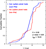
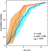
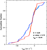
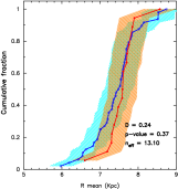
Figure 2: Cumulative distribution function of V mag (upper left panel), stellar ages (upper right panel), $V_{\rm LSR}$ (bottom left), and mean Galactocentric distance (bottom right) for cool and hot PHs.

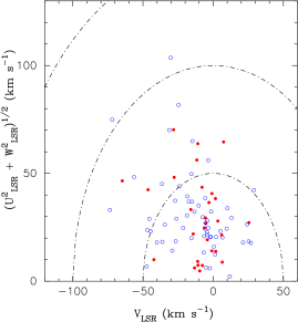
Figure 3: Toomre diagram of the observed stars. Hot PHs are shown by filled red circles while cool PHs are plotted with open blue circles. Dash-dot lines indicate constant total velocities, $V_{\rm Total}=\sqrt{U^{\rm 2}_{\rm LSR}+V^{\rm 2}_{\rm LSR}+W^{\rm 2}_{\rm LSR}}=$ 50, 100, and 150 km s^-1. Median uncertainties for $V_{\rm LSR}$ and $V_{\rm Total}$ are of the order of 0.54 km s^-1.

3 Analysis

3.1 Metallicity distributions

The cumulative distribution functions of the metallicity for the hot and cool PH samples are presented in Figure 4. For guidance, some statistical diagnostics are also given in Table 3. The hatched regions indicate the limits of the cumulative distributions built by considering that all stars have a metallicity of [Fe/H] + $\Delta$[Fe/H] and [Fe/H] - $\Delta$[Fe/H]. A two-sample K-S test shows that the global metallicity distributions of hot- and cool-PHs are similar ($p$-value $\sim$ 20%, K-S statistics $\sim$ 0.24, n_eff $\sim$ 19). In order to account for the uncertainties in the derived metallicities, we proceed as in Sect. 2.4. The significance of the original $p$-value is found to be of only $\sim$ 6.5%, thus confirming the reliability of the result.

We note that a visual inspection of Figure 4 suggests a “deficit” of hot PHs with respect to cool PHs at metallicity values between +0.00 and +0.20 dex, even if the uncertainties in the cumulative distributions are considered. A similar result was found by Maldonado et al. (2015) but based on a smaller sample (only 5 hot PHs and 17 cool PHs). In order to find further confirmation of this possible trend, Maldonado et al. (2015), in their Appendix B, additionally performed a study of the gas-giant planets listed in the Extrasolar Planets Encyclopaedia (Schneider et al., 2011) and the Exoplanet Orbit Database (Wright et al., 2011) without applying any further selection criteria (and therefore mixing different types of stars and planets and with inhomogeneous metallicity determinations). The results from this comparison showed a “deficit” of hot Jupiters at metallicities between -0.50 and +0.00 dex.

In order to test the significance of this possible deficit we repeated the statistical analysis performed before but considering only the stars with metallicities below or equal to +0.20 dex. The K-S test returns in this case a K-S statistic of 0.37 and a low $p$-value of only $\sim$ 0.08 (slightly larger than the usual threshold of 2% for statistical significant difference). Although the samples’ size diminishes significantly, we note that the value of n_eff is still large, $\sim$ 10.5 (the K-S test is reasonably accurate for sample sizes for which n_eff is greater than four ), and the significance of the $p$-value returned by our simulations is of the order of $\sim$ 3%. Our conclusion is that the deficit of hot PHs at low metallicities might be real although it may need further confirmation by analysing larger samples.

We finally note that in our sample there are no hot Jupiters harbouring stars with metallicities below $\sim$ -0.10 dex, whilst cool Jupiters can be found around more metal-poor stars.

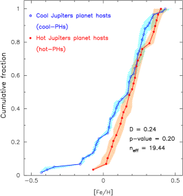
Figure 4: [Fe/H] cumulative frequencies.

Table 3: [Fe/H] statistics of the stellar samples.

$Sample$	$Mean$	$Median$	$Deviation$	$Min$	$Max$	$N$
cool-PHs	0.12	0.18	0.18	-0.43	0.43	59
hot-PHs	0.20	0.20	0.12	-0.07	0.40	29

3.2 Other chemical signatures

In order to find differences in the abundances of other chemical elements besides iron, the cumulative distribution [X/Fe] comparing the abundance distributions of hot- and cool-PHs is shown in Figure 5. Some statistical diagnostics are also presented in Table 4, where the results of a K-S test for each ion are also listed. The tests suggest that there might be differences in the abundances of C i, Si i, S i, and Ca i (slightly larger abundances for the cool PHs). We note that in all these cases our simulations show that the low $p$-values derived are not due to the uncertainties in the derived abundances. It is worth mentioning that Si i and Ca i are $\alpha$ elements and that the $p$-value returned by the K-S test is also very low for Mg i, another $\alpha$ element. On the other hand, very similar abundance distributions are found for Sc i, Cr i, and Mn i, the latter two ions being iron-peak elements.

Figure 5: [X/Fe] cumulative fraction of hot PHs (red continuous line) and cool PHs (blue dash-to-dot line).

Table 4: Comparison between the elemental abundances of hot and cool PHs.

[X/Fe]	Hot PHs		Cool PHs		K-S test
	Median	$\sigma$	Median	$\sigma$	$D$	$p$-value	neff	$p$-sig.
C/O	0.71	0.68	0.68	1.07	0.15	0.95	11.69	0.071
Mg/Si	1.05	0.19	1.10	0.17	0.20	0.40	19.44	0.050
$X_{\alpha}$	-0.02	0.05	0.00	0.05	0.42	$<$ 0.01	19.44	$<$ 0.001
$X_{\rm Fe}$	0.02	0.06	0.02	0.06	0.14	0.81	19.44	0.128
$X_{\rm vol}$	-0.03	0.13	0.02	0.10	0.25	0.16	19.44	0.043
C i	-0.06	0.31	0.04	0.28	0.40	0.01	16.02	0.002
O i	-0.09	0.10	-0.08	0.12	0.30	0.17	12.54	0.018
Na i	0.02	0.11	0.04	0.08	0.20	0.37	19.44	0.047
Mg i	0.00	0.08	0.04	0.08	0.28	0.08	19.44	0.008
Al i	0.05	0.15	0.04	0.07	0.20	0.41	18.88	0.076
Si i	0.00	0.06	0.02	0.04	0.33	0.02	19.44	0.003
S i	-0.04	0.17	0.01	0.14	0.43	$<$ 0.01	18.55	$<$ 0.001
Ca i	-0.06	0.10	-0.02	0.09	0.35	0.01	19.44	0.002
Sc i	-0.02	0.07	-0.02	0.10	0.11	0.98	17.28	0.056
Sc ii	-0.01	0.07	-0.02	0.07	0.14	0.79	19.44	0.081
Ti i	-0.02	0.05	-0.01	0.06	0.16	0.64	19.44	0.085
Ti ii	-0.01	0.07	-0.01	0.08	0.15	0.75	19.44	0.086
V i	0.03	0.07	0.02	0.10	0.16	0.63	19.44	0.074
Cr i	-0.02	0.03	-0.02	0.04	0.11	0.96	19.44	0.044
Cr ii	0.02	0.09	0.05	0.12	0.28	0.07	19.44	0.004
Mn i	0.13	0.13	0.14	0.12	0.13	0.90	19.44	0.112
Co i	-0.02	0.11	-0.03	0.11	0.16	0.65	18.99	0.088
Ni i	-0.01	0.04	0.00	0.04	0.14	0.84	19.44	0.091
Cu i	0.13	0.34	0.06	0.28	0.26	0.27	13.15	0.034
Zn i	0.00	0.14	0.02	0.15	0.13	0.89	19.44	0.080

We therefore grouped the ions into three categories: alpha elements, iron-peak elements, and volatile elements. Following the definitions provided in Mata Sánchez et al. (2014) and Maldonado & Villaver (2017) we considered Mg, Si, Ca, and Ti as alpha elements; Cr, Mn, Co, and Ni as iron-peak elements; and C, O, Na, S, and Zn as volatiles.

The corresponding cumulative functions are shown in Figure 6, where [X_α/Fe], [X_Fe/Fe], and [X_vol/Fe] denote the abundances of alpha, iron-peak, and volatile elements, respectively. The results from the K-S test show no abundance difference in iron elements between hot- and cool PHs. However, the test suggests significant differences when $\alpha$ elements are considered, showing cool PHs to have slightly larger abundances. For volatile elements, the K-S test returns a probability of $\sim$ 16% that both samples have similar distributions, not low enough to claim a statistical significant difference. Possible age effects affecting these results are discussed in Sect. 4.1.

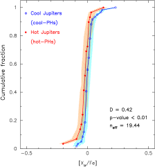
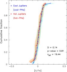
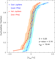
Figure 6: Histogram of cumulative frequencies of [X_α/Fe] (left), [X_Fe/Fe] (middle), and [X_vol/Fe] (right).

Finally, the stellar C/O and Mg/Si ratios were also considered; see Figure 7. These ratios are known to play an important role in constraining the planetary composition (e.g. Bond et al., 2010; Thiabaud et al., 2015; Dorn et al., 2015). No statistically significant differences between hot and cool PHs have been found.

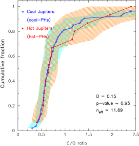
Figure 7: Histogram of cumulative frequencies of C/O (left), and Mg/Si (right).

3.3 Stellar metallicity and planetary properties

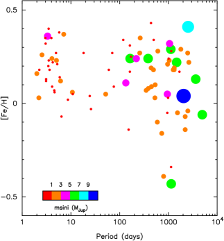
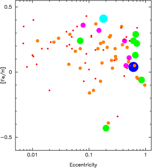
Figure 8: [Fe/H] as a function of the orbital period (left panel) and eccentricity (right panel). Stars are plotted with different colours and increasing sizes with increasing planet minimum mass. Median uncertainties are 0.6 M_Jup for the planetary minimum mass, 0.6 days for the planetary periods, 0.04 for the eccentricities, and 0.02 dex for [Fe/H].

We perform a search for correlations between the stellar abundances and the planet orbital properties. Figure 8 shows the stellar metallicity as a function of the orbital period (left) and versus the planetary eccentricity (right). Colours and symbols, indicate different planetary masses. The Figure shows a lack of massive planets at short orbital periods. We note that all planets (except one) with m${}_{\rm p}\sin i$ larger that 3 M_Jup have a period larger than 100 days. Indeed, most of the planets with m${}_{\rm p}\sin i$ larger than 1 M_Jup have periods larger than 100 days. The Figure also shows that planets at short periods have larger metallicities (in agreement with the results from Sect. 3.1). All stars (except 2) with planets with $P$ $<$ 100 days show metallicities larger than + 0.00 dex. A tendency of higher eccentricities towards more massive planets also seems to be present in the data. Most of the planets with m${}_{\rm p}\sin i$ larger that 3 M_Jup show eccentricities larger than 0.1.

3.4 Comparison with previous works

The absence of massive planets orbiting at short periods around low-metallicity stars in radial velocity surveys was already noted by Udry et al. (2002); Santos et al. (2003); Fischer & Valenti (2005). In a recent work, Jenkins et al. (2017) discuss a tendency of stars with short-period gas giant planets to have higher metallicities than stars with planets at longer periods. Our results also agree with published results based on the analysis of the transit survey planets (e.g. Beaugé & Nesvorný, 2013) where the smallest Kepler planetary candidates orbiting metal-poor stars were found to show a possible period dependency: small planets orbiting metal-poor stars are located at large periods while small planets closer to the star tend to have higher metallicities. On the other hand, the presence of massive gas-giant planets at long orbital periods (even around low-metallicity stars) might be explained if they are mainly formed by gravitational instabilities in the disc (e.g. Dodson-Robinson et al., 2009), a mechanism that does not depend on the metallicity of the primordial disc (Boss, 1997, 2002, 2006).

Dawson & Murray-Clay (2013) find that gas-giant planets at short orbital distances ($a$ $<$ 0.1 au) around metal-poor stars are confined to lower eccentricities while eccentric proto-hot Jupiters undergoing tidal circularization orbit metal-rich stars. A comparison with this work seems complicated given the relatively low number of planet hosts in our sample that are located in the so-called Period Valley, 0.10 - 1.00 au semimajor axis range or 10 days $<$ $P$ $<$ 100 days (e.g. Jones et al., 2003). For this purpose the period-eccentricity diagram of our sample is shown in the upper left panel of Figure 9 where stars are plotted with different colours according to their metallicities. It is clear from this Figure that our planet hosts are concentrated in two different regions of the plot: one of planets with periods $P$ $<$ 10 days and eccentricities lower than 0.1 (with 25 stars); and another of periods $P$ $>$ 50 days and eccentricities larger than $\sim$ 0.05 (with 52 planet-hosts). The “period valley” is also visible in our sample (although showing a narrower gap) with only three planets with periods between 10 and 50 days.

Our results seem to agree qualitatively with Dawson & Murray-Clay (2013). First, for small planets located close to the parent stars (m${}_{\rm p}\sin i$ $<$ 1 M_Jup, $P$ $<$ 10 days), planet-hosts show positive metallicities and their planets have low eccentricities. As in Dawson & Murray-Clay (2013) hot Jupiters are found around metal-rich stars. For the stars in the valley, Dawson & Murray-Clay (2013) find mostly metal-rich planet hosts, with a large range of eccentricities. In this period range our sample contains three stars with positive metallicities, two hosting planets at high eccentricity ($e$ $>$ 0.6) and the other one at low eccentricity ($e$ $<$ 0.01). Finally, as in Dawson & Murray-Clay (2013), for large planetary periods, low- and high-metallicity stars are mixed covering a large range of eccentricities.

Our findings are also in agreement with Adibekyan et al. (2013) who showed that very massive planets with eccentric orbits have longer periods than those with circular orbits and also that most of the planets with long periods orbit around low-metallicity stars. In more recent works, Bashi et al. (2017) and Santos et al. (2017) state that a transition in metallicity at m${}_{\rm p}\sin i$ $\sim$ 5-4 M_Jup may occur, the stars hosting massive gas-giant planets being on average more metal-poor than the stars hosting planets with masses below 5-4 M_Jup. While a tendency of lower metallicities towards higher planetary masses seems to be present in our data, as previously suggested by Ribas & Miralda-Escudé (2007) and Jenkins et al. (2017), we do not find any significant metallicity difference between planet hosts with masses below and above 4 M_Jup (a K-S test returns a probability $\sim$ 99% of planet hosts with masses below and above 4 M_Jup to have similar metallicity distributions). However, it should be noted that our sample and the one discussed in Santos et al. (2017) differ in selection criteria, size, and range of considered planetary masses.

Differences in the eccentricity distribution of planets with masses above and below 4 M_Jup have also been reported. Ribas & Miralda-Escudé (2007) found that massive planets have an eccentricity distribution consistent with that of binary systems. On the other hand, less massive planets have lower eccentricities. A mild tendency of higher eccentricities towards higher planetary masses seems consistent with our data. We performed a K-S on the eccentricity distribution of planets with masses above and below 4 M_Jup. The results confirm the larger eccentricity values of the massive planets ($D$=0.35, $p$-value = 0.05, n_eff = 14.2) in agreement with Ribas & Miralda-Escudé (2007).

3.5 Comparison with brown dwarf results

The findings of the previous subsection can be compared with the results from stars harbouring companions in the brown dwarf regime. Maldonado & Villaver (2017) found that stars harbouring brown dwarfs with (minimum) masses M_C$\sin i$ $<$ 42.5 M_Jup tend to have slightly larger metallicities and lower eccentricities than stars harbouring brown dwarfs in the range M_C$\sin i$ $>$ 42.5 M_Jup. It is interesting to note that hot-PHs, such as stars harbouring the less massive brown dwarfs, tend to have slightly larger metallicities, lower eccentricities, and less massive companions (when compared with cool-PHs). This could suggest a common formation mechanism for hot Jupiters and low-mass brown dwarfs in which metallicity plays a significant role; that is, the core-accretion model. On the other hand, for cool Jupiters and massive brown dwarfs a metallicity dependency does not appear in the data and thus the metal content might not be involved in their formation mechanism. Despite the similarities in metallicity and eccentricity, no further analogies between brown dwarfs and gas-giant planets are found. In particular, the different period distributions should be noted. Only one brown dwarf in the Maldonado & Villaver (2017) sample has a period shorter than 10 days.

3.6 Other chemical signatures and the period-eccentricity distribution

We finally explore the relationships between the planetary position in the period-eccentricity diagrams and the stellar abundances as quantified by the [X_α/Fe], [X_Fe/Fe], [X_vol/Fe] values, as well as the stellar C/O and Mg/Si ratios. The stars are divided into stars with low- and high-[X/Fe] values. Table 5 provides the percentage of low-abundance stars in the population of short and long period planets for each considered abundance. In order to do that we first estimate the [X/Fe] distribution of non-planet host stars. The spectroscopic abundances provided by Maldonado et al. (2015) were used as they were computed using the same methods and similar spectra to those used in this work. In addition, a 3$\sigma$ clipping procedure was done to remove outliers. The corresponding median abundances are 0.00, -0.02, 0.01, 0.54, and 1.05, respectively, for [X_α/Fe], [X_Fe/Fe], [X_vol/Fe], C/O, and Mg/Si. Figure 9 shows the corresponding period-eccentricity plots. Stars are plotted with different colours and symbols depending on whether their [X/Fe] values are below or above the median values derived from the Maldonado et al. (2015) distributions.

For each considered abundance ([X_α/Fe], [X_Fe/Fe], [X_vol/Fe], C/O, and Mg/Si), the percentage of stars with low and high abundances in the population of short- and long-period planets was computed. In order to test the significance of the derived percentages a series of 10⁶ simulations was performed. In each simulation each star was given a new abundance value chosen randomly assuming an underlying Gaussian abundance distribution with the same parameters (mean and sigma) as those derived from the Maldonado et al. (2015) data and the percentage of low-abundance stars was computed. Assuming that the distribution of the simulated percentages of low-abundance stars follows a Gaussian distribution we then compute the probability that the simulated percentage takes the value (within 5%) found when analysing the original data. The results are given in Table 5.

When considering $\alpha$-elements, the low-abundance stars tend to dominate the short-period part of the diagram, in agreement with the results from Sect. 3.2. The percentage of low $\alpha$ abundance stars in the short-period, low-eccentricity part of the diagram is $\sim$ 64%. However, in the long-period, large-eccentricity region, stars with low and high $\alpha$ abundances are well mixed, and the percentage of low-$\alpha$ stars decreases to 40%. The simulations show that the probability of obtaining a distribution with 64% low-$\alpha$ stars in a sample of 25 stars by chance is only $\sim$ 4%. On the other hand, for the long-period, high-eccentricity subsample, the probability of getting 40% low-$\alpha$ stars in a sample of 52 stars is high, of 18.5%, consistent with a random mixture of high and low $\alpha$ abundances.

A similar analysis was performed for iron-peak and volatile elements, as well as for the C/O and Mg/Si ratios. The results are given in Table 5. No trends with the iron-peak, volatiles, or C/O, and Mg/Si ratios seem to be present in the data. We note that a visual inspection of the C/O in Figure 9 reveals only two low-abundance stars in the short-period planets group. However, the percentage of low C/O stars in this group is $\sim$ 15.4%, similar to the one in the long period planets group ($\sim$ 19.2%).

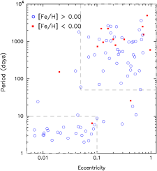
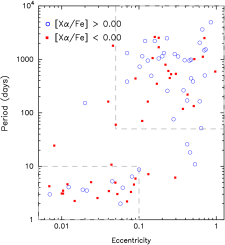
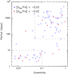
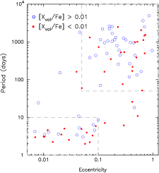
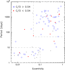
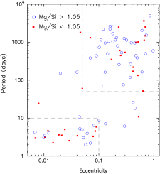
Figure 9: Period vs. eccentricity diagram. Stars are plotted with different colours and symbols according to their corresponding [Fe/H] (top left), X$\alpha$ (top middle), X_Fe (top right) X_vol (bottom left), C/O (bottom middle), and Mg/Si (bottom right) values. Typical uncertainties are 0.6 days (period), 0.04 (eccentricity), 0.02 dex (metallicity, X$\alpha$, and X_Fe), 0.05 dex (X_vol), 0.15 (C/O ratio), and 0.10 (Mg/Si ratio).

Table 5: Fraction of low-abundance stars in the period-eccentricity diagram. Each value is accompanied by its corresponding probability “by chance”.

	$P$ $<$ 10 days, e $<$ 0.1		$P$ $>$ 50 days, e $>$ 0.05
$[X/Fe]$	Fraction (%)	$p$-chance (%)	Fraction (%)	$p$-chance (%)
$X_{\alpha}$	64.0	4.0	40.0	18.5
$X_{\rm Fe}$	28.0	2.6	15.4	$<$ 0.1
$X_{\rm vol}$	56.0	10.4	40.0	16.8
C/O ratio	15.4	1.5	19.1	0.7
Mg/Si ratio	48.0	15.5	32.7	0.1

4 Discussion

The mechanisms involved in the formation of hot Jupiters are nowadays strongly debated (see references in Sect. 1). In the following we discuss the results from the previous Section in the framework of current planet formation and migration models.

4.1 Is our comparison biased?

The first possibility that we should address is whether or not some stellar property is affecting the metal content of any of our samples. That is the reason we performed the analysis in Section 2.4 where we found a tendency of hot PHs to be slightly fainter and younger than cool PHs in our sample.

Haywood (2009) suggested that the observed correlation between the presence of gas-giant planets and high stellar metallicity might be related to a possible galactic inner disc origin of planet hosts. Following this line of reasoning, hints of a correlation between the T_C slopes (i.e., the linear trends between the abundances and the elemental condensation temperature) and the stellar age have been noted in the literature (Adibekyan et al., 2014; Maldonado et al., 2015; Nissen, 2015; Spina et al., 2016). In a recent study, Maldonado & Villaver (2016) found Galactic radial mixing to be the only suitable scenario to explain the observed T_C trends in a large sample of evolved (subgiant and red giant) stars. Adibekyan et al. (2014, 2016) use the stellar R_mean as a proxy of the stellar birthplace finding a weak hint that the T_C trend depends on R_mean, although the authors highlight the complexity of the dependency.

Radial mixing is a secular process and older stars migrate further. Old stars might come from a region with significantly different abundances. As we have seen there is a tendency of hot PHs to be younger than cool PHs. It could be the case that cool PHs show a wider range of metallicities than hot PHs just because they are older. This might be in contradiction with the results from the R_mean distributions analysis. Hot PHs have slightly larger R_mean values and stars at larger Galactocentric distances (from the outer disc) are expected to show lower metallicities (e.g. Lemasle et al., 2008, Fig. 5). However, the differences in R_mean between hot and cool PHs do not seem to be significant.

Therefore, we conclude that we cannot completely rule out the possibility that differences in age and R_mean are affecting the comparison of abundances between both samples.

The fact that hot PHs are slightly fainter than cool PHs should not, to our knowledge, alter the metal content of the stars. Nevertheless, we have explored the $V$ magnitude versus [Fe/H] diagram finding no obvious trend.

We finally explore whether the larger fraction of F-type stars in the hot PHs (24%) sample with respect to the cool PHs sample (7%) might affect our results. Although we do not know of any physical reason why F, G, and K stars might have different abundance distributions we should carefully check that there are no (unknown) systematic effects hidden in the abundance computations that may bias our results. Figure 10 shows the metallicity distribution for the F-, G-, and K-type stars. Although no statistically significant differences are found, a tendency of F-type stars to show lower metallicities (at values of [Fe/H] ¿ 0.1 dex) than G- and K-type stars can be seen. Results from a K-S test provide $D$ = 0.38, $p$-value = 0.11, n_eff = 9.22 when comparing the F and G subsamples. A comparison of the K and G subsamples gives $D$ = 0.26, $p$-value = 0.22, n_eff = 14.81. This shows that if different from G, and K-type stars, the metallicity distribution of F-type stars would be biased towards lower values at high metallicities. It is therefore unlikely that the larger fraction of F-type stars in the hot PHs might explain their higher metallicities when compared with the cool PH sample.

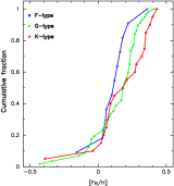
Figure 10: [Fe/H] cumulative frequencies for F-, G-, and K-type stars.

4.2 Metallicity trends and the formation of hot Jupiters

Until very recently, the existence of hot Jupiters involved migration towards the star after the planet is formed in metal-rich discs at large distances from the star, beyond the ice line ($a$ $\gtrsim$ 1-3 au) where solid material is abundant (e.g. Pollack et al., 1996). On the other hand, the in situ formation of hot Jupiters has been largely dismissed mainly due to the lack of sufficient condensate solids in the inner regions of the protoplanetary disk (Lin et al., 1996). However, several recent works have pointed out that this assumption is mainly based on models of the solar nebula that might not apply in general (e.g. Bodenheimer et al., 2000; Boley et al., 2016; Batygin et al., 2016), revisiting whether or not hot Jupiters should necessarily form at large distances from the parent star.

To the very best of our knowledge, the exact dependency of the migration mechanisms proposed so far (disc or high-eccentricity) on the stellar metallicity is still poorly understood. Disc migration might be expected to show some degree of dependence on the stellar metallicity (e.g. Liu et al., 2016), which can be considered a indicator of the disc’s opacity (if as usually assumed no alteration of the disc’s metal content has occurred).

The abundance analysis performed in this work might help us in our understanding of where hot Jupiters form. Until a better understanding of whether migration can alter the metal content of the host stars is achieved, we find it reasonable to assume that if hot Jupiters were formed at large distances from the star and then migrate, cool and hot Jupiters should show similar chemical properties.

We find that more massive planets tend to have larger periods in more eccentric orbits. In agreement with previous works (Dawson & Murray-Clay, 2013; Adibekyan et al., 2013) these stars show a wider range of metallicities. In other words, hot and cool Jupiters seem to constitute two different populations with different properties.

As shown in the previous Section there seems to be a “deficit” of cool Jupiters in the metallicity range +0.00/+0.20 dex. Furthermore, there are no hot Jupiters with metallicities below $\sim$ -0.10 dex. It should be noted that if both cool and hot Jupiters form at large distances from the star, a metallicity dependent migration mechanism should be able to explain this difference.

The data also shows a tendency of cool PHs to show larger values of [X_α/Fe]. The fact that cool PHs show slightly lower metallicity but larger $\alpha$ abundances than hot PHs might also provide important clues regarding planet formation. It has been argued that in order to form a sufficiently massive core, the quantity that should be considered is the surface density of all condensible elements beyond the ice line (Mordasini et al., 2012), especially the $\alpha$ elements O, Si, and Mg (Robinson et al., 2006; Gonzalez, 2009). In particular, it should be noted that Mg and Si have condensation temperatures very similar to iron (Lodders, 2003). It is therefore likely that cool PHs might ‘compensate’ their lower metallicity content with other contributors to allow planetary formation. Along these lines, Adibekyan et al. (2012) found that most of the planet-host stars with low iron content are enhanced by $\alpha$ elements. Figure 11 shows the [X_α/Fe] versus [Fe/H] plane for our sample. While most of our planet hosts are in the metallicity range between -0.1 and +0.4 dex where the tendency [X_α/Fe] versus [Fe/H] seems to be flat, a tendency of higher [X_α/Fe] as we move towards lower metallicities seems to be present in our data in agreement with the results of Adibekyan et al. (2012).

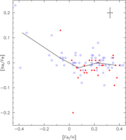
Figure 11: [X_α/Fe] vs. [Fe/H] plane. Hot PHs are shown by filled red circles while cool PHs are plotted with open blue circles. The continuous line shows the mean distribution. Median uncertainties in the derived [X_α/Fe] and [Fe/H] values are also shown.

5 Conclusions

In this work a detailed chemical analysis of a large sample of gas-giant planet hosts is presented. The sample has been divided into stars with cool distant planets and stars with hot Jupiters. Before comparing the two subsamples, a detailed analysis of their stellar properties was performed to control any possible bias affecting our results.

The main results of this work can be summarised as follows:

• Hot PHs show higher metallicities than cool PHs in the metallicity range between +0.00 and +0.20 dex, and no hot Jupiters are found orbiting stars with very low metallicities.

• Hot PHs tend to show lower $\alpha$ abundances than cool PHs.

• Planetary masses of hot Jupiters are typically within m${}_{\rm p}\sin i$ $\sim$ 1 M_Jup and eccentricities do no exceed 0.1.

• Cool PHs have planetary masses significantly larger than 1 M_Jup and a wider range of eccentricities (between 0.05 and 1).

We caution that differences in age might be affecting the comparison of abundances between both samples, as we find that cool PHs might be older than hot PHs. Furthermore, the large fraction of F stars in the hot PHs sample should also be considered.

Our results challenge the traditional view that hot Jupiters form at large distances from the stars and then migrate. While migration mechanisms might alter some planetary properties, such as, for example, the planetary eccentricity, it is unlikely that they change the abundance content of the host star. The data also show that other elements besides iron, such as Mg, Si, or Ti , might play a role in planet formation by compensating the slightly lower metallicity values of cool PHs.

The detailed chemical analysis of samples complementary to the one analysed here, including different planetary types and architectures and different kinds of planet hosts, will help us to expand, confirm, or reject the various trends discussed in this work as well as to achieve a comprehensive view of the planetary formation processes.

Appendix A Additional tables

1]

Table 6: Spectroscopic parameters with uncertainties for the stars measured in this work.

HIP	Sample⋆	Teff	$\log g$	$\xi_{t}$	[Fe/H]	Sp.†	Age	M⋆	R⋆	Kin‡
		(K)	(${\rm cms^{-2}}$)	(${\rm kms^{-1}}$)	(dex)		(Gyr)	(M⊙)	(R⊙)
522	c m	6282 $\pm$ 30	4.16 $\pm$ 0.05	1.54 $\pm$ 0.16	0.07 $\pm$ 0.02	1	2.56 $\pm$ 0.23	1.25 $\pm$ 0.01	1.38 $\pm$ 0.02	D
1292	c	5566 $\pm$ 25	4.69 $\pm$ 0.05	1.27 $\pm$ 0.12	0.11 $\pm$ 0.02	1	0.38 $\pm$ 0.27	0.98 $\pm$ 0.01	0.87 $\pm$ $<$0.01	D
1931	c	5894 $\pm$ 20	4.37 $\pm$ 0.05	1.12 $\pm$ 0.11	0.29 $\pm$ 0.02	1	3.46 $\pm$ 0.94	1.20 $\pm$ 0.04	1.34 $\pm$ 0.14	D
2350	h	5231 $\pm$ 18	4.64 $\pm$ 0.05	0.77 $\pm$ 0.13	0.20 $\pm$ 0.02	2	2.64 $\pm$ 2.66	0.92 $\pm$ 0.02	0.84 $\pm$ 0.02	D
7513	h m	6132 $\pm$ 25	4.07 $\pm$ 0.05	1.41 $\pm$ 0.11	0.06 $\pm$ 0.02	4	3.66 $\pm$ 0.47	1.26 $\pm$ 0.04	1.60 $\pm$ 0.03	D
8770	c m	6057 $\pm$ 20	4.30 $\pm$ 0.04	1.32 $\pm$ 0.10	0.25 $\pm$ 0.02	1	2.64 $\pm$ 0.35	1.22 $\pm$ 0.01	1.30 $\pm$ 0.04	D
9683	c m	5711 $\pm$ 15	4.43 $\pm$ 0.04	1.03 $\pm$ 0.11	0.35 $\pm$ 0.02	1	2.33 $\pm$ 1.05	1.09 $\pm$ 0.01	1.05 $\pm$ 0.03	D
12048	c	5749 $\pm$ 10	4.13 $\pm$ 0.03	1.17 $\pm$ 0.08	0.09 $\pm$ 0.01	1	7.90 $\pm$ 0.23	1.08 $\pm$ 0.01	1.52 $\pm$ 0.04	TR
14954	c	6195 $\pm$ 50	4.32 $\pm$ 0.10	1.56 $\pm$ 0.26	0.10 $\pm$ 0.04	1	3.01 $\pm$ 0.35	1.32 $\pm$ 0.03	1.68 $\pm$ 0.04	D
15527	c	5751 $\pm$ 28	4.39 $\pm$ 0.07	0.79 $\pm$ 0.16	-0.10 $\pm$ 0.02	1	9.72 $\pm$ 0.93	0.93 $\pm$ 0.01	1.10 $\pm$ 0.03	D
16537	c	5181 $\pm$ 15	4.81 $\pm$ 0.04	0.98 $\pm$ 0.16	-0.04 $\pm$ 0.02	1				D
17096	c	5922 $\pm$ 13	4.36 $\pm$ 0.03	1.15 $\pm$ 0.08	-0.16 $\pm$ 0.01	1	7.19 $\pm$ 0.41	0.97 $\pm$ 0.01	1.10 $\pm$ 0.01	D
20199	c	5679 $\pm$ 13	4.40 $\pm$ 0.03	0.98 $\pm$ 0.10	-0.14 $\pm$ 0.01	1	8.39 $\pm$ 1.65	0.90 $\pm$ 0.01	0.95 $\pm$ 0.03	D
20723	c	5687 $\pm$ 18	4.50 $\pm$ 0.04	1.01 $\pm$ 0.11	0.24 $\pm$ 0.02	1	4.96 $\pm$ 1.42	1.05 $\pm$ 0.01	1.08 $\pm$ 0.04	D
21850	c m	5634 $\pm$ 23	4.45 $\pm$ 0.06	1.05 $\pm$ 0.12	0.41 $\pm$ 0.02	1	2.77 $\pm$ 1.59	1.07 $\pm$ 0.01	1.05 $\pm$ 0.04	D
22320	c	5454 $\pm$ 15	4.61 $\pm$ 0.04	0.84 $\pm$ 0.16	0.17 $\pm$ 0.02	1	3.42 $\pm$ 3.07	0.96 $\pm$ 0.02	0.92 $\pm$ 0.04	TR
23889	c	5992 $\pm$ 15	4.08 $\pm$ 0.04	1.38 $\pm$ 0.09	0.27 $\pm$ 0.02	1	3.08 $\pm$ 0.18	1.39 $\pm$ 0.04	1.88 $\pm$ 0.11	D
26394	c	5945 $\pm$ 5	4.35 $\pm$ 0.02	1.14 $\pm$ 0.04	0.04 $\pm$ 0.01	2	4.74 $\pm$ 0.19	1.07 $\pm$ $<$ 0.01	1.15 $\pm$ $<$ 0.01	D
28393	c m (bd)	5277 $\pm$ 28	4.56 $\pm$ 0.06	0.83 $\pm$ 0.20	0.21 $\pm$ 0.03	1	3.95 $\pm$ 3.28	0.92 $\pm$ 0.02	0.87 $\pm$ 0.03	D
31246	h	5355 $\pm$ 25	4.71 $\pm$ 0.06	0.82 $\pm$ 0.21	0.32 $\pm$ 0.03	1	8.51 $\pm$ 2.07	0.94 $\pm$ 0.02	0.98 $\pm$ 0.03	D
31592	c	5236 $\pm$ 108	4.70 $\pm$ 0.29	2.18 $\pm$ 0.50	-0.39 $\pm$ 0.09	1	3.96 $\pm$ 1.27	1.23 $\pm$ 0.12	3.94 $\pm$ 0.18	D
32916	h	5649 $\pm$ 15	4.52 $\pm$ 0.04	0.83 $\pm$ 0.10	0.27 $\pm$ 0.02	3	2.57 $\pm$ 1.78	1.05 $\pm$ 0.02	1.01 $\pm$ 0.04	D
32970	c	6026 $\pm$ 15	4.25 $\pm$ 0.04	1.26 $\pm$ 0.10	0.27 $\pm$ 0.02	1	2.97 $\pm$ 0.19	1.23 $\pm$ 0.01	1.35 $\pm$ 0.04	D
33719	c m	6117 $\pm$ 23	4.33 $\pm$ 0.05	1.30 $\pm$ 0.11	0.18 $\pm$ 0.02	1	2.40 $\pm$ 0.36	1.21 $\pm$ 0.01	1.26 $\pm$ 0.02	D
38558	c m	5645 $\pm$ 15	4.63 $\pm$ 0.04	0.94 $\pm$ 0.14	-0.14 $\pm$ 0.02	1	3.61 $\pm$ 2.14	0.92 $\pm$ 0.02	0.87 $\pm$ 0.02	D
40693	h m	5489 $\pm$ 35	4.62 $\pm$ 0.09	0.96 $\pm$ 0.26	0.02 $\pm$ 0.04	1	1.52 $\pm$ 1.44	0.93 $\pm$ 0.02	0.84 $\pm$ 0.01	D
42214	h	5546 $\pm$ 20	4.61 $\pm$ 0.05	1.19 $\pm$ 0.12	0.26 $\pm$ 0.02	1	1.17 $\pm$ 1.00	1.03 $\pm$ 0.02	0.93 $\pm$ 0.02	D
42446	c	4993 $\pm$ 35	4.00 $\pm$ 0.10	0.90 $\pm$ 0.22	0.29 $\pm$ 0.05	1	5.50 $\pm$ 0.80	1.25 $\pm$ 0.05	2.37 $\pm$ 0.15	D
42723	c m	6046 $\pm$ 15	4.27 $\pm$ 0.04	1.36 $\pm$ 0.10	0.05 $\pm$ 0.02	1	4.43 $\pm$ 0.62	1.21 $\pm$ 0.04	1.57 $\pm$ 0.06	D
43177	h	6116 $\pm$ 15	4.34 $\pm$ 0.04	1.32 $\pm$ 0.10	0.23 $\pm$ 0.02	1	1.77 $\pm$ 0.29	1.23 $\pm$ 0.01	1.23 $\pm$ 0.03	D
43686	h	5691 $\pm$ 20	4.32 $\pm$ 0.05	1.14 $\pm$ 0.11	0.35 $\pm$ 0.02	1	3.74 $\pm$ 2.58	1.13 $\pm$ 0.08	1.27 $\pm$ 0.26	TR
44291	h	5439 $\pm$ 28	4.59 $\pm$ 0.06	0.84 $\pm$ 0.18	0.38 $\pm$ 0.03	1	1.01 $\pm$ 0.87	1.00 $\pm$ 0.01	0.90 $\pm$ 0.02	D
47007	c m	5984 $\pm$ 13	4.46 $\pm$ 0.04	1.15 $\pm$ 0.09	0.24 $\pm$ 0.01	1	1.16 $\pm$ 0.51	1.17 $\pm$ 0.01	1.12 $\pm$ 0.03	D
47202	h	5492 $\pm$ 13	4.57 $\pm$ 0.03	0.91 $\pm$ 0.11	0.35 $\pm$ 0.02	2	2.38 $\pm$ 1.78	1.02 $\pm$ 0.01	0.95 $\pm$ 0.03	D
48711	h	5980 $\pm$ 15	4.20 $\pm$ 0.03	1.28 $\pm$ 0.07	0.16 $\pm$ 0.02	2	3.94 $\pm$ 0.78	1.19 $\pm$ 0.04	1.37 $\pm$ 0.13	D
48739	c	5854 $\pm$ 13	4.36 $\pm$ 0.03	1.10 $\pm$ 0.08	-0.05 $\pm$ 0.01	1	4.64 $\pm$ 1.51	1.00 $\pm$ 0.01	1.02 $\pm$ 0.04	D
48780	c	6473 $\pm$ 73	4.24 $\pm$ 0.14	1.73 $\pm$ 0.33	0.22 $\pm$ 0.05	1	1.52 $\pm$ 0.45	1.41 $\pm$ 0.03	1.56 $\pm$ 0.07	D
52409	c m	5782 $\pm$ 20	4.58 $\pm$ 0.04	1.02 $\pm$ 0.12	0.31 $\pm$ 0.02	1	2.69 $\pm$ 1.09	1.11 $\pm$ 0.01	1.10 $\pm$ 0.03	D
54195	c	5817 $\pm$ 28	4.05 $\pm$ 0.06	1.28 $\pm$ 0.12	0.34 $\pm$ 0.03	1	3.89 $\pm$ 0.59	1.31 $\pm$ 0.07	1.80 $\pm$ 0.14	D
55409	c	5708 $\pm$ 20	4.46 $\pm$ 0.05	1.01 $\pm$ 0.12	-0.06 $\pm$ 0.02	1	6.05 $\pm$ 2.16	0.95 $\pm$ 0.02	0.97 $\pm$ 0.04	D
55664	c	5378 $\pm$ 30	4.65 $\pm$ 0.08	0.82 $\pm$ 0.25	0.43 $\pm$ 0.04	1	1.80 $\pm$ 1.69	0.98 $\pm$ 0.02	0.91 $\pm$ 0.03	D
57172	c	5212 $\pm$ 23	4.69 $\pm$ 0.05	0.77 $\pm$ 0.21	0.27 $\pm$ 0.03	1	1.09 $\pm$ 1.05	0.93 $\pm$ 0.01	0.83 $\pm$ 0.01	TR
57370	h	5350 $\pm$ 10	4.67 $\pm$ 0.03	0.93 $\pm$ 0.12	0.09 $\pm$ 0.02	2	0.89 $\pm$ 0.86	0.93 $\pm$ 0.01	0.83 $\pm$ 0.01	D
58237	h	5025 $\pm$ 25	4.65 $\pm$ 0.06	0.95 $\pm$ 0.18	0.07 $\pm$ 0.03	2	2.25 $\pm$ 2.47	0.83 $\pm$ 0.02	0.75 $\pm$ 0.02	D
58263	h	6435 $\pm$ 70	4.32 $\pm$ 0.13	1.62 $\pm$ 0.19	0.14 $\pm$ 0.04	2	1.60 $\pm$ 0.55	1.34 $\pm$ 0.02	1.46 $\pm$ 0.06	D
60644	c	6130 $\pm$ 15	4.26 $\pm$ 0.04	1.34 $\pm$ 0.09	0.05 $\pm$ 0.01	1	2.81 $\pm$ 0.39	1.15 $\pm$ 0.01	1.20 $\pm$ 0.03	D
61595	h	5848 $\pm$ 15	4.31 $\pm$ 0.04	1.18 $\pm$ 0.09	0.21 $\pm$ 0.02	1	3.91 $\pm$ 1.68	1.11 $\pm$ 0.02	1.18 $\pm$ 0.09	D
62534	c	5468 $\pm$ 15	4.50 $\pm$ 0.04	0.85 $\pm$ 0.12	-0.43 $\pm$ 0.01	1	11.42 $\pm$ 0.21	0.77 $\pm$ 0.01	0.79 $\pm$ $<$ 0.01	TR
64457	c	5232 $\pm$ 80	4.61 $\pm$ 0.20	0.86 $\pm$ 0.38	0.18 $\pm$ 0.07	1	2.53 $\pm$ 2.66	0.87 $\pm$ 0.02	0.79 $\pm$ 0.02	D
64459	c	5761 $\pm$ 10	4.01 $\pm$ 0.02	1.21 $\pm$ 0.08	-0.34 $\pm$ 0.01	1	10.61 $\pm$ 0.31	0.93 $\pm$ 0.01	1.52 $\pm$ 0.03	TR
65808	c	5664 $\pm$ 15	4.46 $\pm$ 0.04	1.05 $\pm$ 0.09	0.22 $\pm$ 0.02	1	6.28 $\pm$ 0.77	1.03 $\pm$ 0.01	1.10 $\pm$ 0.03	D
66047	c m	5934 $\pm$ 10	4.28 $\pm$ 0.02	1.21 $\pm$ 0.07	-0.03 $\pm$ 0.01	1	6.26 $\pm$ 0.34	1.04 $\pm$ 0.01	1.19 $\pm$ 0.03	D
66192	h	5797 $\pm$ 73	4.21 $\pm$ 0.17	1.26 $\pm$ 0.24	0.12 $\pm$ 0.06	3	4.73 $\pm$ 0.83	1.25 $\pm$ 0.07	1.88 $\pm$ 0.13	D
67275	h	6704 $\pm$ 50	4.59 $\pm$ 0.08	1.58 $\pm$ 0.26	0.36 $\pm$ 0.04	1	0.11 $\pm$ 0.01	1.41 $\pm$ $<$ 0.01	1.32 $\pm$ $<$ 0.01	D
70695	c	5690 $\pm$ 15	4.52 $\pm$ 0.03	0.99 $\pm$ 0.11	-0.05 $\pm$ 0.01	1	5.93 $\pm$ 1.99	0.95 $\pm$ 0.02	0.96 $\pm$ 0.03	TR
71395	c m	5000 $\pm$ 30	4.69 $\pm$ 0.08	1.10 $\pm$ 0.21	0.09 $\pm$ 0.03	1	1.03 $\pm$ 1.13	0.83 $\pm$ 0.01	0.73 $\pm$ 0.01	D
72339	h	5430 $\pm$ 10	4.64 $\pm$ 0.02	0.84 $\pm$ 0.09	0.06 $\pm$ 0.01	2	1.84 $\pm$ 1.74	0.94 $\pm$ 0.02	0.85 $\pm$ 0.02	D
74500	c m	5753 $\pm$ 15	4.37 $\pm$ 0.04	1.09 $\pm$ 0.10	0.27 $\pm$ 0.02	1	5.48 $\pm$ 0.48	1.10 $\pm$ 0.01	1.21 $\pm$ 0.03	D
77517	h	5064 $\pm$ 38	4.68 $\pm$ 0.09	0.69 $\pm$ 0.38	0.18 $\pm$ 0.04	1	5.30 $\pm$ 4.22	0.86 $\pm$ 0.02	0.81 $\pm$ 0.02	TR
77838	h	6475 $\pm$ 140	4.50 $\pm$ 0.27	1.50 $\pm$ 0.25	0.03 $\pm$ 0.08	3	1.80 $\pm$ 0.89	1.33 $\pm$ 0.04	1.50 $\pm$ 0.08	D
78169	c	5914 $\pm$ 18	4.42 $\pm$ 0.05	1.17 $\pm$ 0.10	0.08 $\pm$ 0.02	1	0.98 $\pm$ 0.75	1.09 $\pm$ 0.01	1.01 $\pm$ 0.02	D
78521	c	5631 $\pm$ 40	4.64 $\pm$ 0.09	1.13 $\pm$ 0.22	0.32 $\pm$ 0.04	1	1.76 $\pm$ 1.60	1.05 $\pm$ 0.02	0.99 $\pm$ 0.04	D
80337	c	5874 $\pm$ 15	4.56 $\pm$ 0.03	1.18 $\pm$ 0.09	0.03 $\pm$ 0.01	1	0.31 $\pm$ 0.20	1.07 $\pm$ 0.01	0.96 $\pm$ $<$ 0.01	D
80680	c	6196 $\pm$ 38	4.38 $\pm$ 0.08	1.39 $\pm$ 0.22	0.24 $\pm$ 0.04	1	0.57 $\pm$ 0.42	1.24 $\pm$ 0.02	1.19 $\pm$ 0.03	D
81022	h	5904 $\pm$ 20	4.19 $\pm$ 0.05	1.28 $\pm$ 0.09	0.24 $\pm$ 0.02	1	4.07 $\pm$ 0.36	1.20 $\pm$ 0.03	1.39 $\pm$ 0.08	D
83983	c	5744 $\pm$ 23	4.33 $\pm$ 0.05	1.18 $\pm$ 0.15	0.24 $\pm$ 0.03	1	6.46 $\pm$ 0.81	1.10 $\pm$ 0.03	1.33 $\pm$ 0.07	D
88414	c	4848 $\pm$ 55	4.73 $\pm$ 0.14	0.70 $\pm$ 0.44	0.28 $\pm$ 0.06	1	3.90 $\pm$ 3.72	0.82 $\pm$ 0.02	0.75 $\pm$ 0.02	D
90004	h	5612 $\pm$ 13	4.50 $\pm$ 0.03	0.97 $\pm$ 0.11	-0.07 $\pm$ 0.01	1	11.08 $\pm$ 0.58	0.90 $\pm$ 0.01	1.03 $\pm$ 0.03	D
90593	c	5820 $\pm$ 15	4.37 $\pm$ 0.04	1.16 $\pm$ 0.11	0.28 $\pm$ 0.02	1	4.18 $\pm$ 0.86	1.14 $\pm$ 0.03	1.25 $\pm$ 0.09	D
91258	h	5498 $\pm$ 25	4.67 $\pm$ 0.05	0.73 $\pm$ 0.19	0.23 $\pm$ 0.03	3	1.03 $\pm$ 0.92	1.00 $\pm$ 0.02	0.90 $\pm$ 0.02	D
94645	h	6185 $\pm$ 20	4.34 $\pm$ 0.04	1.33 $\pm$ 0.11	0.12 $\pm$ 0.02	1	1.42 $\pm$ 0.58	1.20 $\pm$ 0.01	1.19 $\pm$ 0.03	D
97336	h m	5839 $\pm$ 20	4.54 $\pm$ 0.04	0.91 $\pm$ 0.11	0.13 $\pm$ 0.02	3	5.17 $\pm$ 0.71	1.07 $\pm$ 0.01	1.15 $\pm$ 0.03	D
97546	c	6051 $\pm$ 15	4.20 $\pm$ 0.03	1.34 $\pm$ 0.09	0.03 $\pm$ 0.01	1	4.57 $\pm$ 0.37	1.12 $\pm$ 0.01	1.28 $\pm$ 0.05	D
99115	c	5597 $\pm$ 20	4.08 $\pm$ 0.05	1.09 $\pm$ 0.12	0.23 $\pm$ 0.02	1	8.62 $\pm$ 0.48	1.08 $\pm$ 0.02	1.53 $\pm$ 0.08	TR
99711	c	5069 $\pm$ 23	4.74 $\pm$ 0.05	0.92 $\pm$ 0.19	0.04 $\pm$ 0.02	1	0.31 $\pm$ 0.24	0.84 $\pm$ 0.01	0.73 $\pm$ 0.01	D
101806	c	5849 $\pm$ 15	4.23 $\pm$ 0.03	1.21 $\pm$ 0.08	0.19 $\pm$ 0.01	1	5.55 $\pm$ 0.63	1.14 $\pm$ 0.03	1.39 $\pm$ 0.05	TR
102125	c	5901 $\pm$ 18	4.03 $\pm$ 0.04	1.27 $\pm$ 0.11	0.13 $\pm$ 0.02	1	4.33 $\pm$ 0.82	1.27 $\pm$ 0.09	1.79 $\pm$ 0.21	D
107985	c m	5764 $\pm$ 15	4.61 $\pm$ 0.04	1.01 $\pm$ 0.09	0.17 $\pm$ 0.01	1	0.74 $\pm$ 0.62	1.08 $\pm$ 0.01	0.97 $\pm$ 0.02	D
109378	c	5521 $\pm$ 15	4.38 $\pm$ 0.05	0.97 $\pm$ 0.12	0.19 $\pm$ 0.02	1	9.43 $\pm$ 0.71	0.96 $\pm$ 0.01	1.07 $\pm$ 0.02	D
110852	h	6254 $\pm$ 30	4.38 $\pm$ 0.06	1.24 $\pm$ 0.15	0.18 $\pm$ 0.02	1	0.48 $\pm$ 0.33	1.25 $\pm$ 0.02	1.19 $\pm$ 0.03	D
111143	c	5886 $\pm$ 10	4.08 $\pm$ 0.03	1.28 $\pm$ 0.08	0.05 $\pm$ 0.01	1	6.71 $\pm$ 0.16	1.11 $\pm$ 0.01	1.52 $\pm$ 0.04	D
113044	c	5944 $\pm$ 20	4.08 $\pm$ 0.05	1.28 $\pm$ 0.11	0.18 $\pm$ 0.02	1	3.96 $\pm$ 0.47	1.29 $\pm$ 0.04	1.71 $\pm$ 0.04	D
113137	c	5814 $\pm$ 10	4.18 $\pm$ 0.03	1.21 $\pm$ 0.07	0.18 $\pm$ 0.01	1	6.32 $\pm$ 0.72	1.13 $\pm$ 0.03	1.47 $\pm$ 0.03	D
113238	c	5468 $\pm$ 25	4.65 $\pm$ 0.05	0.85 $\pm$ 0.20	0.34 $\pm$ 0.03	1	1.14 $\pm$ 0.99	1.01 $\pm$ 0.02	0.91 $\pm$ 0.01	TR
113357	h	5839 $\pm$ 40	4.38 $\pm$ 0.10	1.30 $\pm$ 0.23	0.22 $\pm$ 0.04	1	3.17 $\pm$ 1.32	1.11 $\pm$ 0.02	1.11 $\pm$ 0.03	D
113421	h m	5656 $\pm$ 18	4.43 $\pm$ 0.05	1.01 $\pm$ 0.12	0.37 $\pm$ 0.02	1	4.43 $\pm$ 0.57	1.07 $\pm$ 0.01	1.10 $\pm$ 0.01	D
115662	c	5869 $\pm$ 20	4.27 $\pm$ 0.04	1.15 $\pm$ 0.09	-0.07 $\pm$ 0.01	1	6.75 $\pm$ 0.88	0.99 $\pm$ 0.01	1.10 $\pm$ 0.04	D
BD-103166	h	5449 $\pm$ 43	4.64 $\pm$ 0.10	0.93 $\pm$ 0.26	0.40 $\pm$ 0.05	1	1.38 $\pm$ 1.25	1.00 $\pm$ 0.02	0.91 $\pm$ 0.02	D

Table 6: Continued.

2]

Table 7: Derived abundances [X/H]

HIP	C i	O i	Na i	Mg i	Al i	Si i	S i	Ca i	Sc i	Sc ii	Ti i	Ti ii	V i	Cr i	Cr ii	Mn i	Co i	Ni i	Cu i	Zn i
522	0.00	-0.06	0.16	0.01	0.08	0.10	0.07	0.06	0.13	0.07	0.01	-0.01	0.09	0.06	0.05	0.10	-0.02	0.03	-0.29	-0.07
	0.06	0.05	0.08	0.11	0.07	0.01	0.34	0.05	0.05	0.07	0.03	0.06	0.08	0.04	0.06	0.05	0.04	0.02	0.04	0.09
1292	0.25	0.07	0.04	0.06	0.09	0.10	0.14	0.08	0.01	0.03	0.07	0.05	0.16	0.10	0.14	0.25	0.06	0.05	0.07	0.16
	0.14	0.05	0.07	0.03	0.04	0.02	0.10	0.05	0.07	0.05	0.05	0.05	0.04	0.04	0.07	0.05	0.05	0.02	0.04	0.17
1931	0.27	0.20	0.30	0.29	0.32	0.32	0.30	0.27	0.25	0.26	0.24	0.28	0.28	0.26	0.44	0.49	0.21	0.31	0.25	0.33
	0.17	0.03	0.06	0.03	0.01	0.01	0.12	0.04	0.05	0.05	0.03	0.05	0.02	0.03	0.13	0.04	0.04	0.02	0.11	0.16
2350			0.24	0.19	0.22	0.21	0.29	0.06	0.24	0.19	0.22	0.18	0.30	0.21	0.18	0.39	0.24	0.21		0.17
			0.04	0.05	0.02	0.02	0.09	0.07	0.11	0.05	0.06	0.05	0.05	0.04	0.09	0.06	0.05	0.03		0.06
7513	-0.10	0.04	0.05	0.03	-0.11	0.08	0.06	0.07		0.02	-0.01	0.00	0.03	-0.02	0.10	0.06	-0.31	-0.01	-0.33	0.05
	0.11	0.05	0.14	0.13	0.20	0.02	0.15	0.06		0.05	0.03	0.07	0.07	0.06	0.06	0.05	0.33	0.03	0.21	0.06
8770	0.17	0.16	0.30	0.28	0.24	0.32	0.21	0.22	0.25	0.22	0.21	0.17	0.25	0.22	0.32	0.37	0.17	0.27	0.32	0.04
	0.06	0.05	0.03	0.06	0.01	0.02	0.14	0.04	0.05	0.04	0.02	0.05	0.04	0.03	0.09	0.04	0.05	0.02	0.09	0.05
9683	0.46	0.23	0.52	0.44	0.40	0.37	0.36	0.25	0.30	0.41	0.33	0.36	0.35	0.31	0.39	0.61	0.36	0.40	0.96	0.47
	0.13	0.05	0.05	0.04	0.03	0.01	0.07	0.05	0.03	0.05	0.04	0.07	0.03	0.04	0.05	0.05	0.03	0.02	0.20	0.21
12048	0.03	0.08	0.05	0.20	0.14	0.10	0.04	0.09	0.00	0.05	0.08	0.10	0.05	0.09	0.20	0.17	0.02	0.07	0.10	0.13
	0.08	0.04	0.03	0.03	0.01	0.01	0.11	0.05	0.03	0.05	0.03	0.05	0.03	0.03	0.08	0.04	0.05	0.02	0.18	0.17
14954	-0.25	0.01	0.11	0.07	-0.10	0.09	0.18	-0.16		0.04	0.09	0.16	0.19	0.10	0.24	0.29	0.18	0.11	0.01	0.17
	0.13	0.06	0.13	0.08	0.04	0.05	0.14	0.10		0.06	0.04	0.06	0.05	0.05	0.07	0.06	0.04	0.04	0.04	0.13
15527	-0.12	-0.04	-0.20	-0.11	-0.09	-0.11	0.13	-0.08	-0.22	-0.11	-0.14	-0.05	-0.15	-0.13	-0.26	-0.19	-0.15	-0.18	-0.24	0.57
	0.23	0.06	0.03	0.16	0.04	0.02	0.25	0.05	0.05	0.05	0.04	0.07	0.03	0.04	0.24	0.06	0.08	0.02	0.02	0.71
16537	0.31	-0.08	-0.12	-0.09	-0.07	-0.05		-0.09	-0.06	-0.15	0.02	-0.04	0.07	-0.02	-0.05	0.03	-0.07	-0.11	-0.08	-0.11
	0.05	0.10	0.05	0.05	0.04	0.02		0.05	0.09	0.05	0.06	0.05	0.05	0.05	0.05	0.05	0.06	0.03	0.06	0.06
17096	-0.10	-0.10	-0.17	-0.11	-0.14	-0.14	-0.17	-0.12	-0.11	-0.21	-0.17	-0.14	-0.22	-0.19	-0.12	-0.22	-0.27	-0.21	-0.24	-0.31
	0.08	0.06	0.04	0.07	0.01	0.01	0.12	0.04	0.05	0.04	0.02	0.04	0.03	0.03	0.06	0.05	0.05	0.02	0.08	0.04
20199	0.07	0.02	-0.14	0.05	0.03	-0.07	0.01	-0.09	-0.13	-0.08	-0.02	-0.04	-0.10	-0.15	-0.12	-0.19	-0.11	-0.18	-0.14	-0.09
	0.15	0.05	0.02	0.07	0.02	0.02	0.14	0.05	0.03	0.04	0.04	0.05	0.03	0.04	0.05	0.06	0.05	0.02	0.02	0.10
20723	0.23	0.10	0.36	0.31	0.28	0.26	0.29	0.15	0.20	0.24	0.23	0.22	0.26	0.21	0.26	0.45	0.25	0.26	0.59	0.29
	0.08	0.05	0.04	0.03	0.02	0.02	0.08	0.05	0.06	0.04	0.04	0.05	0.03	0.04	0.05	0.05	0.05	0.02	0.12	0.18
21850	0.56	0.23	0.54	0.49	0.46	0.41	0.45	0.28	0.38	0.42	0.40	0.37	0.43	0.37	0.43	0.68	0.43	0.45	0.67	0.50
	0.17	0.10	0.06	0.06	0.02	0.02	0.04	0.04	0.06	0.05	0.05	0.07	0.04	0.04	0.05	0.07	0.05	0.03	0.04	0.19
22320	0.38	0.09	0.12	0.19	0.23	0.17	0.19	0.07	0.15	0.21	0.19	0.17	0.21	0.13	0.07	0.33	0.16	0.15	0.34	0.19
	0.23	0.16	0.04	0.04	0.02	0.01	0.05	0.05	0.06	0.05	0.05	0.07	0.04	0.05	0.07	0.07	0.05	0.03	0.06	0.11
23889	0.23	0.21	0.47	0.33	0.32	0.33	0.26	0.24	0.30	0.31	0.25	0.26	0.25	0.22	0.32	0.45	0.33	0.34	0.45	0.29
	0.06	0.05	0.03	0.04	0.06	0.01	0.09	0.04	0.03	0.04	0.02	0.04	0.04	0.04	0.08	0.05	0.05	0.02	0.11	0.14
26394	-0.09		0.08	0.08	0.03	0.04	0.10	0.04	0.00	-0.03	-0.01	0.01	-0.03	0.03	0.05	0.09	-0.03	0.02		-0.03
	0.04		0.03	0.04	0.01	0.01	0.04	0.04	0.04	0.04	0.02	0.04	0.03	0.03	0.05	0.05	0.04	0.02		0.07
28393	0.49	0.11	0.35	0.27	0.30	0.26	0.34	0.12	0.27	0.17	0.26	0.18	0.34	0.21	0.21	0.57	0.24	0.24	0.65	0.28
	0.11	0.05	0.06	0.05	0.02	0.02	0.07	0.06	0.10	0.05	0.06	0.07	0.05	0.05	0.04	0.07	0.04	0.03	0.11	0.03
31246	0.64	0.21	0.41	0.35	0.38	0.32	0.16	0.14	0.36	0.34	0.37	0.32	0.45	0.27	0.33	0.64	0.37	0.34	0.75	0.35
	0.11	0.17	0.08	0.05	0.05	0.02	0.11	0.05	0.12	0.06	0.05	0.07	0.05	0.04	0.04	0.06	0.05	0.03	0.02	0.07
31592	0.73	-0.33	-0.51	-0.26	-0.46	-0.44	0.30	-0.81	0.02	-0.61	-0.13	0.04	0.14	-0.20	0.09	-0.12	-0.03	-0.27	-0.05	-0.18
	0.05	0.06	0.10	0.20	0.03	0.07	0.05	0.12	0.24	0.11	0.09	0.11	0.11	0.10	0.08	0.07	0.20	0.06	0.05	0.30
32916			0.24	0.32	0.31	0.25	-0.08	0.21	0.24	0.21	0.25	0.23	0.28	0.28	0.22	0.41	0.19	0.26		0.05
			0.02	0.07	0.03	0.02	0.13	0.04	0.04	0.05	0.04	0.05	0.04	0.04	0.06	0.06	0.05	0.02		0.04
32970	0.27	0.13	0.41	0.30	0.32	0.34	0.29	0.25	0.24	0.26	0.24	0.24	0.27	0.25	0.37	0.48	0.22	0.32	0.35	0.17
	0.06	0.05	0.04	0.05	0.01	0.01	0.14	0.04	0.04	0.04	0.02	0.05	0.03	0.03	0.08	0.04	0.04	0.02	0.04	0.04
33719	0.00	0.06	0.24	0.16	0.18	0.21	0.12	0.19	0.07	0.15	0.13	0.17	0.14	0.15	0.24	0.25	0.06	0.17	0.08	0.03
	0.07	0.05	0.04	0.06	0.01	0.02	0.14	0.05	0.05	0.04	0.03	0.04	0.03	0.03	0.07	0.04	0.05	0.02	0.11	0.04
38558	-0.13	-0.04	-0.22	-0.12	-0.16	-0.14	-0.15	-0.13	-0.24	-0.20	-0.14	-0.13	-0.11	-0.13	-0.10	-0.16	-0.23	-0.21	-0.35	0.00
	0.08	0.04	0.03	0.05	0.02	0.02	0.18	0.05	0.05	0.04	0.04	0.04	0.07	0.04	0.05	0.05	0.05	0.02	0.02	0.28
40693	0.49	-0.06	-0.04	0.07	0.08	0.01	0.00	-0.03	-0.05	0.00	0.06	0.01	0.09	0.00	-0.03	0.15	-0.01	-0.02	0.34	0.02
	0.05	0.20	0.05	0.03	0.02	0.01	0.04	0.05	0.09	0.04	0.05	0.05	0.04	0.04	0.04	0.05	0.05	0.02	0.31	0.13
42214	0.13	0.17	0.32	0.26	0.31	0.29	0.30	0.20	0.21	0.23	0.23	0.22	0.32	0.22	0.25	0.41	0.25	0.25	0.58	0.34
	0.08	0.10	0.06	0.03	0.02	0.02	0.08	0.05	0.07	0.05	0.05	0.05	0.04	0.04	0.05	0.06	0.05	0.02	0.23	0.25
42446	0.87	0.26	0.32	0.33	0.34	0.36	0.54	0.10	0.40	0.37	0.31	0.48	0.36	0.22	0.40	0.70	0.35	0.34	1.05	0.40
	0.30	0.24	0.08	0.05	0.05	0.04	0.18	0.07	0.22	0.07	0.09	0.12	0.09	0.07	0.06	0.10	0.06	0.04	0.06	0.06
42723	0.08	0.00	0.14	0.10	0.08	0.11	0.01	0.07	0.06	0.02	0.05	0.05	0.05	0.03	0.11	0.15	-0.01	0.05	-0.02	-0.08
	0.09	0.04	0.04	0.07	0.01	0.01	0.13	0.04	0.04	0.04	0.02	0.04	0.04	0.03	0.08	0.05	0.04	0.02	0.08	0.04
43177	0.02	0.03	0.15	0.22	0.21	0.25	0.07	0.25	0.20	0.19	0.20	0.20	0.21	0.18	0.26	0.26	0.10	0.20	-0.01	-0.06
	0.06	0.04	0.05	0.07	0.02	0.01	0.14	0.05	0.05	0.04	0.03	0.04	0.03	0.03	0.08	0.06	0.04	0.02	0.01	0.06
43686	0.48	0.16	0.36	0.44	0.44	0.41	0.31	0.31	0.33	0.39	0.36	0.38	0.39	0.31	0.34	0.55	0.35	0.36	0.43	0.40
	0.14	0.09	0.06	0.07	0.02	0.02	0.07	0.05	0.07	0.05	0.04	0.06	0.03	0.04	0.06	0.05	0.05	0.03	0.04	0.28
44291	0.52	0.18	0.46	0.30	0.44	0.40	0.46	0.19	0.37	0.41	0.37	0.36	0.43	0.35	0.40	0.78	0.41	0.40	0.79	0.36
	0.18	0.13	0.06	0.18	0.06	0.01	0.10	0.05	0.10	0.05	0.05	0.07	0.04	0.05	0.06	0.06	0.05	0.03	0.05	0.04
47007	0.20	0.16	0.30	0.24	0.22	0.26	0.21	0.20	0.19	0.20	0.20	0.21	0.21	0.24	0.34	0.40	0.17	0.24	0.19	0.24
	0.07	0.06	0.02	0.03	0.01	0.01	0.12	0.04	0.02	0.04	0.02	0.04	0.03	0.03	0.08	0.04	0.04	0.02	0.08	0.19
47202	0.12		0.55	0.43	0.49	0.46	0.23	0.22	0.43	0.42	0.35	0.37	0.44	0.35	0.37	0.70	0.47	0.44		0.44
	0.05		0.05	0.05	0.03	0.02	0.04	0.05	0.07	0.05	0.05	0.06	0.04	0.04	0.06	0.06	0.05	0.02		0.03
48711	0.06		0.19	0.20	0.22	0.20	-0.01	0.15	0.17	0.15	0.12	0.15	0.18	0.14	0.19	0.20	0.09	0.18		0.15
	0.04		0.12	0.04	0.01	0.02	0.18	0.04	0.04	0.04	0.02	0.04	0.04	0.04	0.05	0.07	0.06	0.02		0.07
48739	-0.03	-0.01	-0.05	-0.01	-0.09	-0.05	-0.11	-0.01	-0.16	-0.16	-0.08	-0.10	-0.05	-0.05	0.12	-0.04	-0.16	-0.11	-0.22	-0.24
	0.06	0.04	0.02	0.06	0.03	0.01	0.09	0.04	0.05	0.05	0.03	0.04	0.05	0.03	0.17	0.06	0.04	0.02	0.02	0.04
48780	-0.26	-0.10	0.32	0.08		0.25	0.03	0.26		0.14	0.27	0.13	0.31	0.30	0.16	0.30	0.46	0.20	0.02	0.27
	0.17	0.05	0.14	0.15		0.03	0.24	0.06		0.06	0.06	0.06	0.26	0.07	0.09	0.07	0.04	0.04	0.04	0.14
52409	0.29	0.19	0.36	0.35	0.34	0.33	0.33	0.21	0.24	0.36	0.29	0.32	0.32	0.27	0.34	0.57	0.31	0.33	0.46	0.37
	0.08	0.08	0.06	0.03	0.01	0.01	0.06	0.05	0.04	0.05	0.03	0.06	0.03	0.04	0.06	0.05	0.05	0.02	0.08	0.19
54195	0.26	0.17	0.48	0.43	0.42	0.39	0.46	0.28	0.31	0.38	0.34	0.32	0.41	0.30	0.48	0.67	0.38	0.40	0.62	0.08
	0.07	0.04	0.02	0.04	0.03	0.02	0.06	0.04	0.06	0.05	0.03	0.06	0.03	0.04	0.15	0.08	0.05	0.02	0.17	0.12
55409	0.02	-0.03	-0.09	0.05	-0.02	-0.03	-0.08	-0.04	-0.13	-0.08	-0.05	-0.05	-0.07	-0.06	0.01	-0.07	-0.09	-0.10	-0.13	-0.05
	0.06	0.04	0.02	0.05	0.04	0.02	0.12	0.04	0.08	0.05	0.04	0.04	0.03	0.04	0.06	0.08	0.06	0.02	0.02	0.15
55664	0.47	0.26	0.37	0.47	0.53	0.47	0.56	0.26	0.55	0.51	0.50	0.49	0.56	0.39	0.51	0.71	0.51	0.46	1.21	0.55
	0.19	0.07	0.06	0.05	0.08	0.01	0.08	0.05	0.11	0.06	0.05	0.09	0.06	0.05	0.05	0.09	0.05	0.03	0.09	0.06
57172	0.69	0.05	0.30	0.26	0.33	0.26	0.34	0.09	0.35	0.26	0.33	0.26	0.39	0.25	0.27	0.56	0.31	0.28	0.80	0.26
	0.05	0.14	0.07	0.05	0.04	0.02	0.08	0.06	0.12	0.05	0.06	0.08	0.06	0.05	0.05	0.07	0.05	0.03	0.14	0.07
57370			-0.03	0.03	0.18	0.06	0.35	0.06	0.00	-0.02	0.09	0.06	0.11	0.10	0.10	0.15	0.00	0.01		-0.07
			0.02	0.04	0.16	0.01	0.05	0.05	0.06	0.04	0.05	0.04	0.04	0.04	0.04	0.04	0.04	0.02		0.06
58237			0.02	-0.07	0.09	0.06	0.42	-0.01	0.05	-0.09	0.05	0.01	0.16	0.09	0.05	0.17	0.02	0.03		0.00
			0.05	0.05	0.04	0.03	0.06	0.07	0.12	0.07	0.09	0.07	0.09	0.06	0.09	0.07	0.05	0.04		0.12
58263			0.20	0.09	-0.10	0.12	-0.02	0.05		0.13	0.12	0.14	0.12	0.13	0.25	0.11	0.09	0.11		-0.21
			0.12	0.11	0.04	0.03	0.18	0.09		0.06	0.04	0.06	0.09	0.04	0.06	0.06	0.04	0.03		0.04
60644	-0.02	-0.02	0.04	0.02	-0.03	0.09	-0.02	0.08	0.03	-0.08	-0.01	-0.03	0.03	0.01	0.09	0.04	-0.19	0.00	-0.21	-0.18
	0.04	0.03	0.08	0.09	0.04	0.01	0.16	0.05	0.05	0.04	0.03	0.04	0.05	0.04	0.06	0.05	0.14	0.02	0.01	0.05
61595	0.25	0.13	0.35	0.29	0.28	0.26	0.22	0.17	0.17	0.23	0.18	0.20	0.19	0.19	0.41	0.46	0.19	0.24	0.33	0.32
	0.08	0.04	0.02	0.03	0.02	0.01	0.10	0.04	0.06	0.05	0.03	0.05	0.02	0.03	0.17	0.07	0.04	0.02	0.23	0.23
62534	-0.05	0.06	-0.33	-0.12	-0.12	-0.24	-0.20	-0.27	-0.25	-0.31	-0.16	-0.18	-0.27	-0.42	-0.37	-0.53	-0.33	-0.41	-0.49	-0.20
	0.06	0.05	0.03	0.08	0.02	0.01	0.05	0.05	0.04	0.05	0.05	0.04	0.05	0.04	0.04	0.06	0.06	0.02	0.03	0.10
64457	0.73	0.12	0.26	0.22	0.26	0.15	0.39	0.08	0.30	0.10	0.28	0.11	0.35	0.20	0.10	0.44	0.21	0.16	0.43	0.19
	0.05	0.14	0.05	0.05	0.06	0.02	0.06	0.05	0.11	0.06	0.06	0.07	0.05	0.05	0.05	0.06	0.04	0.03	0.03	0.06
64459	-0.25	-0.14	-0.33	-0.17	-0.22	-0.25	-0.30	-0.22	-0.35	-0.32	-0.25	-0.24	-0.37	-0.36	-0.28	-0.48	-0.39	-0.38	-0.50	-0.34
	0.06	0.05	0.05	0.07	0.02	0.01	0.14	0.05	0.05	0.04	0.03	0.04	0.03	0.03	0.06	0.05	0.05	0.02	0.08	0.12
65808	0.31	0.14	0.25	0.27	0.22	0.23	0.23	0.12	0.18	0.20	0.15	0.19	0.19	0.18	0.26	0.39	0.19	0.22	0.42	0.30
	0.10	0.07	0.03	0.05	0.02	0.02	0.08	0.05	0.06	0.04	0.04	0.05	0.04	0.04	0.05	0.05	0.05	0.02	0.14	0.21
66047	-0.07	-0.02	0.04	0.01	-0.01	0.01	-0.07	0.00	-0.09	-0.10	-0.06	-0.07	-0.07	-0.05	0.01	0.04	-0.09	-0.05	-0.09	-0.04
	0.06	0.04	0.04	0.05	0.01	0.01	0.13	0.04	0.05	0.04	0.02	0.04	0.03	0.03	0.08	0.04	0.04	0.02	0.04	0.12
66192	0.06		0.09	0.15	-0.10	0.08	-0.15	0.02	0.05	0.15	0.08	0.24	0.05	0.16	0.37	0.03	-0.05	0.14		0.21
	0.05		0.05	0.04	0.19	0.04	0.15	0.07	0.11	0.06	0.04	0.06	0.06	0.04	0.16	0.12	0.12	0.03		0.18
67275	-0.01		0.28	0.10		0.33	0.18	0.29		0.44	0.36	0.25	0.52	0.44	0.23	0.53		0.39	0.07	0.56
	0.05		0.04	0.20		0.03	0.20	0.07		0.06	0.08	0.08	0.07	0.11	0.14	0.06		0.04	0.06	0.06
70695	0.02	-0.11	-0.05	0.02	0.03	-0.04	-0.04	-0.07	-0.11	-0.07	-0.03	-0.03	-0.03	-0.08	-0.07	0.02	-0.08	-0.09	-0.03	-0.01
	0.09	0.09	0.03	0.04	0.03	0.02	0.07	0.05	0.03	0.04	0.04	0.04	0.04	0.04	0.05	0.05	0.05	0.02	0.02	0.09
71395	0.62	0.21	0.03	-0.05	0.10	0.11		-0.01	0.14	-0.05	0.12	0.02	0.24	0.13	0.01	0.25	0.05	0.02	0.24	-0.05
	0.07	0.14	0.09	0.05	0.06	0.03		0.08	0.15	0.07	0.10	0.09	0.09	0.06	0.06	0.07	0.05	0.05	0.05	0.06
72339			0.02	0.04	0.07	0.03	0.10	0.00	0.01	0.02	0.08	0.07	0.09	0.08	0.08	0.15	0.03	0.03		0.16
			0.02	0.05	0.02	0.01	0.05	0.05	0.06	0.05	0.05	0.05	0.04	0.04	0.07	0.04	0.05	0.02		0.24
74500	0.32	0.18	0.41	0.35	0.34	0.32	0.28	0.20	0.23	0.29	0.26	0.26	0.27	0.23	0.55	0.49	0.27	0.30	0.62	0.42
	0.10	0.05	0.05	0.04	0.02	0.01	0.08	0.05	0.03	0.05	0.03	0.06	0.03	0.04	0.24	0.06	0.05	0.02	0.16	0.25
77517	0.85	0.21	0.20	0.18	0.39	0.25		-0.01	0.38	0.26	0.35	0.27	0.40	0.14	0.23	0.39	0.24	0.18	0.94	0.27
	0.07	0.15	0.07	0.05	0.06	0.03		0.08	0.18	0.07	0.09	0.09	0.09	0.06	0.06	0.08	0.05	0.04	0.39	0.11
77838	-0.69		-0.38	-0.03	-0.50	-0.20	-0.42	-0.46		-0.07	0.00	-0.15	0.08	0.01	-0.17	0.05	-0.23	-0.04		-0.01
	0.05		0.12	0.04	0.04	0.07	0.03	0.14		0.12	0.05	0.09	0.06	0.10	0.15	0.08	0.15	0.04		0.11
78169	-0.01	0.00	0.01	0.11	0.04	0.08	0.02	0.09	0.02	-0.02	0.04	0.01	0.00	0.06	0.17	0.11	-0.06	0.02	-0.16	-0.16
	0.05	0.08	0.03	0.07	0.01	0.01	0.12	0.04	0.05	0.04	0.02	0.05	0.03	0.03	0.10	0.06	0.08	0.02	0.06	0.06
78521	0.95	0.07	0.24	0.34	0.40	0.30	0.30	0.23	0.56	0.34	0.39	0.36	0.44	0.27	0.13	0.48	0.38	0.30	0.58	0.28
	0.80	0.14	0.11	0.03	0.02	0.02	0.03	0.06	0.10	0.05	0.05	0.07	0.04	0.04	0.05	0.06	0.05	0.04	0.09	0.11
80337	0.07	-0.06	-0.14	-0.01	-0.02	-0.01	-0.07	0.05		-0.06	0.03	0.02	0.05	0.02	0.19	-0.03	-0.12	-0.08	-0.26	-0.14
	0.21	0.03	0.03	0.04	0.02	0.01	0.15	0.04		0.04	0.03	0.05	0.03	0.03	0.17	0.04	0.04	0.02	0.02	0.09
80680	0.25	0.08	0.34	0.20	0.25	0.26	0.20	0.23	0.27	0.26	0.23	0.21	0.42	0.18	0.29	0.35	0.77	0.25	-0.08	0.28
	0.13	0.05	0.06	0.08	0.01	0.02	0.28	0.04	0.11	0.06	0.04	0.06	0.06	0.04	0.09	0.06	0.46	0.02	0.06	0.16
81022	0.22	0.15	0.34	0.29	0.29	0.29	0.28	0.21	0.23	0.27	0.21	0.24	0.27	0.21	0.33	0.42	0.23	0.27	0.37	0.33
	0.09	0.04	0.02	0.03	0.01	0.02	0.08	0.04	0.04	0.04	0.02	0.04	0.03	0.03	0.11	0.04	0.05	0.02	0.13	0.20
83983	0.39	0.07	0.28	0.35	0.34	0.24	0.52	0.22	0.25	0.39	0.26	0.24	0.32	0.22	0.17	0.37	0.25	0.25	0.50	0.24
	0.13	0.05	0.04	0.03	0.01	0.02	0.29	0.05	0.08	0.17	0.04	0.05	0.07	0.04	0.05	0.09	0.05	0.03	0.09	0.17
88414	1.27	0.35	0.38	0.04	0.33	0.26		0.11	0.62	0.21	0.34	0.22	0.67	0.32	0.16	0.53	0.33	0.30	1.09	0.32
	0.08	0.15	0.14	0.06	0.06	0.05		0.11	0.25	0.08	0.11	0.11	0.11	0.08	0.09	0.11	0.06	0.05	0.32	0.09
90004	0.13	0.11	0.01	0.14	0.16	0.03	0.00	-0.02	0.02	0.02	0.09	0.10	0.04	-0.08	-0.07	-0.08	0.00	-0.08	-0.02	0.10
	0.19	0.06	0.08	0.04	0.03	0.02	0.06	0.04	0.05	0.05	0.04	0.05	0.04	0.04	0.05	0.06	0.05	0.02	0.06	0.16
90593	0.32	0.13	0.43	0.36	0.35	0.33	0.34	0.23	0.25	0.32	0.27	0.28	0.30	0.25	0.47	0.50	0.32	0.33	0.77	0.41
	0.10	0.09	0.05	0.03	0.02	0.01	0.08	0.04	0.06	0.05	0.03	0.05	0.03	0.03	0.19	0.05	0.04	0.02	0.37	0.21
91258			0.24	0.18	0.24	0.19	0.12	0.10	0.21	0.28	0.23	0.22	0.24	0.22	0.33	0.36	0.26	0.22		0.09
			0.02	0.14	0.02	0.02	0.09	0.05	0.05	0.09	0.05	0.04	0.04	0.04	0.07	0.07	0.08	0.03		0.04
94645	0.02	0.02	0.16	0.06	0.06	0.17	0.07	0.14	0.11	-0.01	0.07	0.04	0.11	0.11	0.19	0.19	-0.10	0.11	-0.14	0.03
	0.08	0.03	0.07	0.07	0.01	0.01	0.16	0.05	0.04	0.04	0.03	0.05	0.04	0.04	0.06	0.05	0.12	0.02	0.06	0.14
97336	-0.26		0.10	0.13	0.04	0.10	-0.07	0.08	0.07	0.20	0.08	0.17	0.09	0.10	0.17	0.19	0.03	0.10		0.03
	0.05		0.03	0.03	0.05	0.02	0.13	0.05	0.07	0.09	0.03	0.04	0.04	0.03	0.06	0.08	0.06	0.02		0.09
97546	-0.06	-0.05	0.06	0.03	0.00	0.06	-0.07	0.05	0.03	-0.06	-0.01	-0.02	-0.02	-0.01	0.07	0.07	-0.09	0.01	-0.21	-0.16
	0.05	0.04	0.04	0.07	0.01	0.01	0.16	0.04	0.05	0.04	0.02	0.04	0.04	0.03	0.06	0.05	0.06	0.02	0.03	0.05
99115	0.49	0.24	0.26	0.41	0.36	0.34	0.56	0.22	0.18	0.35	0.28	0.23	0.23	0.18	0.22	0.32	0.18	0.24	0.51	0.36
	0.13	0.04	0.04	0.04	0.02	0.03	0.09	0.05	0.06	0.08	0.05	0.07	0.04	0.04	0.07	0.06	0.04	0.03	0.11	0.27
99711	0.56	-0.04	0.05	-0.04	0.06	0.01		-0.06	0.08	-0.08	0.09	0.00	0.20	0.08	0.01	0.18	0.03	-0.01	0.19	-0.02
	0.06	0.10	0.07	0.05	0.04	0.02		0.06	0.12	0.06	0.08	0.08	0.07	0.06	0.07	0.06	0.06	0.04	0.04	0.05
101806	0.24	0.15	0.31	0.28	0.28	0.25	0.19	0.17	0.19	0.24	0.16	0.21	0.17	0.15	0.72	0.35	0.19	0.22	0.42	0.23
	0.10	0.05	0.02	0.03	0.01	0.01	0.13	0.04	0.02	0.04	0.03	0.05	0.03	0.03	0.49	0.04	0.05	0.02	0.16	0.14
102125	0.14	0.14	0.25	0.16	0.17	0.18	0.17	0.13	0.10	0.12	0.07	0.10	0.08	0.08	0.24	0.29	0.04	0.13	0.15	-0.02
	0.08	0.04	0.04	0.05	0.05	0.01	0.12	0.04	0.12	0.05	0.02	0.05	0.04	0.04	0.07	0.06	0.04	0.02	0.04	0.08
107985	-0.01	0.07	0.06	0.19	0.15	0.16	0.15	0.12	0.11	0.12	0.18	0.17	0.19	0.16	0.19	0.34	0.12	0.15	0.23	0.16
	0.06	0.06	0.08	0.03	0.02	0.01	0.07	0.04	0.05	0.05	0.03	0.05	0.04	0.04	0.07	0.05	0.05	0.02	0.02	0.16
109378	0.17	0.19	0.23	0.36	0.33	0.26	0.29	0.14	0.20	0.20	0.24	0.20	0.23	0.16	0.24	0.44	0.18	0.18	0.54	0.38
	0.10	0.06	0.02	0.03	0.02	0.02	0.07	0.05	0.04	0.05	0.05	0.06	0.04	0.04	0.05	0.07	0.05	0.02	0.21	0.20
110852	0.09	-0.02	0.18	0.13	0.00	0.17	0.05	0.15	0.25	0.04	0.14	0.08	0.18	0.18	0.28	0.22	-0.04	0.14	0.01	-0.06
	0.08	0.03	0.05	0.07	0.01	0.02	0.17	0.05	0.04	0.04	0.04	0.05	0.09	0.04	0.14	0.04	0.11	0.02	0.02	0.04
111143	0.06	0.03	0.15	0.12	0.10	0.10	-0.02	0.10	0.05	0.02	0.03	0.03	0.04	0.00	0.11	0.15	0.01	0.06	0.02	0.07
	0.05	0.07	0.04	0.04	0.01	0.01	0.13	0.05	0.05	0.04	0.02	0.04	0.04	0.03	0.07	0.06	0.04	0.02	0.06	0.16
113044	0.12	0.09	0.31	0.21	0.21	0.24	0.13	0.22	0.17	0.16	0.15	0.17	0.17	0.14	0.28	0.31	0.11	0.20	0.16	0.03
	0.06	0.03	0.03	0.05	0.04	0.02	0.11	0.05	0.06	0.04	0.02	0.06	0.03	0.03	0.10	0.04	0.05	0.02	0.14	0.04
113137	0.19	0.13	0.28	0.26	0.27	0.23	0.17	0.17	0.14	0.19	0.18	0.18	0.18	0.16	0.29	0.32	0.18	0.21	0.35	0.25
	0.05	0.03	0.02	0.03	0.02	0.01	0.08	0.04	0.04	0.05	0.03	0.05	0.02	0.03	0.08	0.05	0.04	0.02	0.14	0.23
113238	0.39	0.15	0.46	0.41	0.41	0.35	0.46	0.19	0.35	0.38	0.34	0.37	0.40	0.29	0.41	0.60	0.39	0.39	0.89	0.41
	0.20	0.12	0.05	0.05	0.03	0.02	0.06	0.05	0.09	0.05	0.05	0.07	0.04	0.05	0.04	0.06	0.05	0.03	0.05	0.05
113357	0.27	0.19	0.27	0.28	0.23	0.20	0.12	0.11	0.16	0.15	0.20	0.22	0.23	0.20	0.43	0.36	0.20	0.22	0.52	0.28
	0.12	0.06	0.03	0.05	0.01	0.01	0.10	0.04	0.04	0.04	0.03	0.06	0.03	0.03	0.27	0.05	0.05	0.02	0.36	0.28
113421	0.23	0.21	0.44	0.46	0.44	0.35	0.33	0.28	0.29	0.37	0.36	0.35	0.36	0.31	0.40	0.62	0.35	0.38	0.79	0.44
	0.05	0.09	0.05	0.08	0.05	0.02	0.15	0.05	0.04	0.05	0.04	0.07	0.04	0.04	0.07	0.07	0.05	0.03	0.15	0.13
115662	0.02	0.00	-0.07	-0.01	-0.03	-0.04	-0.10	-0.06	-0.08	-0.13	-0.09	-0.10	-0.10	-0.05	-0.01	0.28	-0.10	-0.09	-0.19	-0.05
	0.08	0.05	0.04	0.07	0.01	0.01	0.14	0.04	0.05	0.05	0.03	0.04	0.05	0.04	0.06	0.31	0.05	0.02	0.02	0.14
BD-103166	0.86	0.21	0.55	0.42	0.48	0.42	0.39	0.26	0.47	0.42	0.46	0.38	0.54	0.34	0.40	0.80	0.46	0.43	1.07	0.43
	0.33	0.17	0.07	0.05	0.06	0.01	0.13	0.06	0.10	0.06	0.05	0.08	0.05	0.05	0.04	0.06	0.05	0.03	0.05	0.07

Table 7: continued.