Resonance oscillation of a damped driven simple pendulum

Abstract

The resonance characteristics of a driven damped harmonic oscillator are well known. Unlike harmonic oscillators which are guided by parabolic potentials, a simple pendulum oscillates under sinusoidal potentials. The problem of an undamped pendulum has been investigated to a great extent. However, the resonance characteristics of a driven damped pendulum have not been reported so far due to the difficulty in solving the problem analytically. In the present work we report the resonance characteristics of a driven damped pendulum calculated numerically. The results are compared with the resonance characteristics of a damped driven harmonic oscillator. The work can be of pedagogic interest too as it reveals the richness of driven damped motion of a simple pendulum in comparison to and how strikingly it differs from the motion of a driven damped harmonic oscillator. We confine our work only to the nonchaotic regime of pendulum motion.

I Introduction

The motion of a simple pendulum has the same equation as the motion of a particle in a sinusoidal potential. And the motion of the simple pendulum with very small amplitude $x$ (so that $\sin x$ can be safely approximated as $x$) is equivalent to that of a harmonic oscillator. However, as the amplitude becomes larger, the motion of the simple pendulum differs from that of a harmonic oscillator. The natural frequency of oscillation of a harmonic oscillator ($\omega_{0}=\sqrt{\frac{k}{m}}$) is independent of its amplitude, with $m$ as the mass of the oscillator and $k$ is the stiffness constant of the spring. However, since a simple pendulum with large amplitude is different from a harmonic oscillator its frequency of oscillation is not independent of the amplitude of its free oscillation. The period or the frequency, $\omega$, of oscillation of a freely oscillating pendulum of finite amplitude, $x_{0}$, is given in terms of an elliptic integral of the first kind and has been given in many text books, as for exampleSommerfeld ; Kittel ; Marion . The frequencies in terms of simple series expansions have also been givenKittel ; Marion and there are many attempts to improve upon the series expansion in order to get to as close as the exact (elliptic integral) value using only few terms, to cite a fewKidd ; Lima ; Rajesh ; Johannessen ; Belendez ; Salas . For comparison of the frequency of oscillation of harmonic oscillator, $\omega_{0}$, and various expresssions for the frequency, $\omega_{1}$, of oscillations of a simple pendulum we use the expressions used by Kittel, et. al.Kittel

$$\frac{\omega_{1}}{\omega_{0}}\approx 1-\frac{x_{0}^{2}}{16}$$ (1)

and the expression arrived at by Beléndez, et. al.Belendez

$$\frac{\omega_{1}}{\omega_{0}}\approx\frac{1}{4}\left(1+\sqrt{\cos\frac{x_{0}}{2}}\right)^{2}$$ (2)

in addition to the exact resultBelendez ,

$$\frac{\omega_{1}}{\omega_{0}}=\frac{\pi}{2K(k)},$$ (3)

where

$$K(k)=\int_{0}^{\frac{\pi}{2}}\frac{d\phi}{\sqrt{1-k\sin^{2}\phi}}$$ (4)

and

$$k=\sin^{2}\frac{x_{0}}{2}$$ (5)

and plotted in Fig. 1, using standard tablesAbramowitz for the elliptic integrals (1.4). It is to be noted that whereas the frequency of free oscillation of a simple harmonic oscillator is independent of amplitude, the frequency of free oscillation of a simple pendulum decreases with its amplitude.

It is also well known that if a harmonic oscillator is driven by an external periodic drive of frequency $\omega$, then the oscillator responds with larger and larger amplitude $x_{0}$ as $\omega\rightarrow\omega_{0}$ and the amplitude becomes infinitely large at $\omega=\omega_{0}$. The condition $\omega=\omega_{0}$ is termed as the resonance condition. Note, however, that a simple pendulum cannot have a similar resonance oscillation at a fixed frequency $\omega=\omega_{0}$ as $\omega(x_{0})$ is not independent of $x_{0}$.

When the harmonic oscillator is (viscous) damped so that it satisfies the equation of motionMarion ; Kleppner

$$\frac{d^{2}x}{dt^{2}}+\gamma\frac{dx}{dt}+\omega_{0}^{2}x=0,$$ (6)

the oscillator, for small damping coefficient $\gamma<2\omega_{0}$, oscillates with displacement

$$x(t)=Ae^{\frac{-\gamma t}{2}}\cos(\omega_{1}t+\phi),$$ (7)

with the frequency of oscillation $\omega_{1}=\sqrt{\omega_{0}^{2}-\frac{\gamma^{2}}{2}}$ and diminishing amplitude $Ae^{-\frac{\gamma t}{2}}$, where $A$ and $\phi$ are arbitrary constants. Notice again that even though frequency of oscillation depends on the damping factor $\gamma$, it remains fixed for all time, independent of the (diminishing) amplitude. The motion of (under)damped pendulum can be described by

$$\frac{d^{2}x}{dt^{2}}+\gamma\frac{dx}{dt}+\omega_{0}^{2}\sin x=0.$$ (8)

An approximate solution has been derived by JohannessenJohannessen1 . The approximate solution compares quite well with the numerical solution. The solution is oscillatory in nature with diminishing amplitude as time progresses, Fig. 1 of Ref.Johannessen1 . The time periods of oscillations are plotted in Fig. 3 of the same refrence as a function of time. One can clearly notice that initially the frequency of oscillations are small but keep increasing with time and the frequency approaches the value appropriate for the damped harmonic oscillator, $\omega_{1}=\sqrt{\omega_{0}^{2}-\frac{\gamma^{2}}{2}}$. This is as it should be because as the amplitude of oscillation approaches zero the motion of simple pendulum becomes closer to that of a simple harmonic oscillator.

The above description reiterates the well-known result that, in presence of damping, the harmonic oscillator as well as the simple pendulum asymptotically approach the stationary state $x(t\rightarrow\infty)=0$. However, if the damped harmonic oscillator is, in addition, subjected to a periodic forcing $F(t)=F_{0}\cos\omega t$, then the equation of motion

$$\frac{d^{2}x}{dt^{2}}+\gamma\frac{dx}{dt}+\omega_{0}^{2}x=\frac{F_{0}}{m}\cos\omega t$$ (9)

has a solution

$$x(t)=x_{0}\cos(\omega t+\phi),$$ (10)

with

$$x_{0}=\frac{F_{0}}{m}\frac{1}{((\omega^{2}-\omega_{0}^{2})^{2}+(\omega\gamma)^{2})^{\frac{1}{2}}}$$ (11)

and

$$\phi=\tan^{-1}(\frac{\gamma\omega}{\omega^{2}-\omega_{0}^{2}}),$$ (12)

is the phase difference between $F(t)$ and the response $x(t)$. Owing to the presence of damping a mean power loss of

$$P=\frac{F_{0}^{2}}{2m}\frac{\gamma\omega}{(\omega^{2}-\omega_{0}^{2})^{2}+(\omega\gamma)^{2}}$$ (13)

occurs. $P$ shows a peak exactly at the frequency $\omega=\omega_{0}$, even though the amplitude peaks at a lower frequency $\omega=\sqrt{\omega_{0}^{2}-\frac{\gamma^{2}}{2}}$. $P$ becomes maximum at $\omega=\omega_{0}$ because the phase difference is $\frac{\pi}{2}$ at this frequency. One can take this frequency $\omega=\omega_{0}$ as the resonance frequency of the forced damped harmonic oscillator. Obviously, the resonance frequency is independent of the damping coefficient or the amplitude of oscillation. The corresponding resonance condition for a damped simple pendulum driven by a periodic force does not have a known analytical expression. We, therefore, numerically obtain the resonance frequency of the forced damped simple pendulum as discussed in the following.

II Resonance Frequency

We investigate the behavior of a forced damped simple pendulum in the present work. In particular, we explore the resonance behavior of such a pendulum by calculating the corresponding mean power loss or equivalently the hysteresis loss. We, in fact, investigate the equivalent problem of motion of an underdamped particle in a sinusoidal potential under the influence of an external periodic force $F(t)=F_{0}\cos\omega t$.

The equation of motion in a periodic potential $V(x)=-\sin x$ is given by (in dimensionless form)

$$\frac{d^{2}x}{dt^{2}}+\gamma\frac{dx}{dt}-\cos x=F_{0}\cos\omega t.$$ (14)

Note that this is exactly the equation of a damped driven simple pendulum if one identifies the angular displacement $\theta=x-\frac{\pi}{2}$. By solving this equation we obtain the mean hysteresis loop, its area, and the amplitudes of the corresponding trajectories $x(t)$ in order to characterize the resonance behavior of the system. We identify, as explained earlier, the resonance frequency as one for which the hysteresis loop area is the largest and calculate the corresponding mean amplitude $\overline{x_{0}}$ of oscillation $x(t)$. The mean hysteresis loop area is just the integral $\int Fdx$ over a large number $N$ of periods of $F(t)$ and calculate the average for one cycle of $F$. This quantity is again averaged over $M$ initial conditions $x(t=0)$ but with $v(t=0)=\frac{dx}{dt}(t=0)=0$, giving the mean hysteresis loop area $\overline{A}$, for various values of frequency $\omega$ for a given $\gamma$. We set $F_{0}=0.2$ throughout in this work except in the inset of Fig. 2. We keep the dimensionless mean amplitude $F_{0}$ small so that the pendulum always remain in the nonchaotic regime. We, thus, identify the frequency $\overline{\omega_{0}}$ which gives the largest hysteresis loop area. The corresponding mean amplitude of oscillation $\overline{x_{0}}$ is also calculated. Fig. 2 gives the plot of the resonance frequency $\overline{\omega_{0}}$ versus the mean amplitude $\overline{x_{0}}$. Each point on the plot corresponds to a fixed value of $\gamma$. For comparison, we also plot the resonance frequency $\omega=\omega_{0}$ of oscillation of damped driven harmonic oscillator in the same graph. Also plotted in the same graph is the exact frequency of free ($\gamma=0$) oscillation of the simple pendulum as a guide to the eye. A similar graph is plotted for drive amplitude $F_{0}=0.1$ as an inset to Fig. 2.

Figure 1: The figure shows the frequency of oscillation $\omega_{1}$ as a function of initial position $x_{0}$ for an undamped simple pendulum. As is shown in the figure, notice that the approximations as obtained by Kittel and Beléndez depart from the exact result at large amplitudes. Also, shown in the figure (by the dash-dotted horizontal line) is the corresponding frequency of oscillation $\omega_{0}$ of an driven-damped harmonic oscillator as a function of initial position $x_{0}$.

In Fig. 2 at least three qualitatively different regions can be clearly identified. One, in the intermediate range $0.165\leq\gamma\leq 0.38$ of $\gamma$, the obtained graph shows the usual tendency of increasing resonance frequency as the amplitude of oscillation decreases, as though to approach the harmonic oscillator limit, as $\gamma$ increases. And the tendency is more so for the smaller drive amplitude $F_{0}=0.1$ as shown in the inset of the figure. Of course, the range of $\gamma$ in this case does not lie in $0.165\leq\gamma\leq 0.38$ but $0.099\leq\gamma\leq 0.28$. Two, for large $\gamma>0.38$, the obtained $\overline{\omega_{0}}$ decreases rapidly with decreasing amplitude $\overline{x_{0}}$ as $\gamma$ increases. $\overline{\omega_{0}}$ thus moves away from the harmonic oscillator limit of resonance frequency $\omega_{0}$. In both these regions of $\gamma$ the resonance frequencies remain lower than the free oscillation frequencies. And thirdly, in the small $\gamma$ regime, the resonance frequency abruptly drops to a small value just below $\gamma\approx 0.165$, thus we get a disjoint branch of the resonance amplitude frequency curve. Thereafter $\overline{\omega_{0}}$ decreases much slowly with increasing $\overline{x_{0}}$. The slow decrease of $\overline{\omega_{0}}$ allows the curve to ultimately cross the amplitude-frequency curve of free oscillation of the simple pendulum. Thus, at smaller $\gamma$ values the resonance frequency $\overline{\omega_{0}}$ becomes larger than the free oscillation frequency. In the following, we discuss the resonance oscillations in the three regions of $\gamma$ separately.

Figure 2: The figure shows the plot of the resonance frequency $\overline{\omega_{0}}$ versus the mean amplitude $\overline{x_{0}}$ of the damped-driven pendulum with each point corresponding to a particular value of damping $\gamma$ (a few of them labelled) for a forcing amplitude $F_{0}=0.2$. The inset shows the same but with a forcing amplitude $F_{0}=0.1$. Also shown, in both the main plot as well as in the inset, are the exact result of the frequency of oscillation $\omega_{1}$ of an undamped simple pendulum (by broken line) and (by the dash-dotted horizontal line) the corresponding resonance frequency of oscillation $\omega_{0}$ of an driven-damped harmonic oscillator.

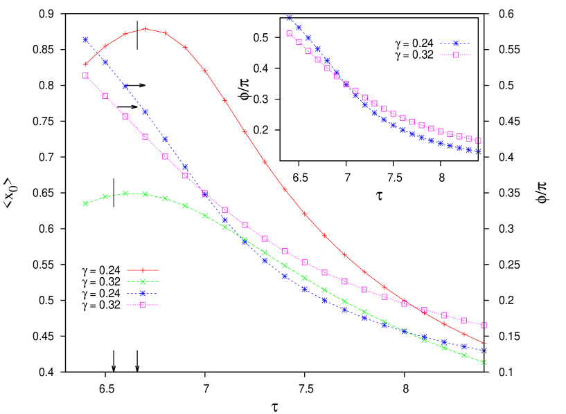
Figure 3: The figure shows the variation of the amplitude of the ensemble averaged hysteresis loop and the phase of the loop as a function of the driving period $\tau$. Note that the two graphs indicated by the horizontal arrows (y-axis label is towards the right hand side) signify the phase of the loop for the two $\gamma$ values as indicated. The phase variation as a function of driving period is replotted in the inset. The right vertical arrow and the right vertical line on $<{x_{0}}>$ indicates the resonant period, $\tau_{0}$ = $6.66$ for $\gamma=0.24$ whereas the left vertical arrow and the left vertical line on $<{x_{0}}>$ is for $\gamma=0.32$ with $\tau_{0}$ = $6.542$.

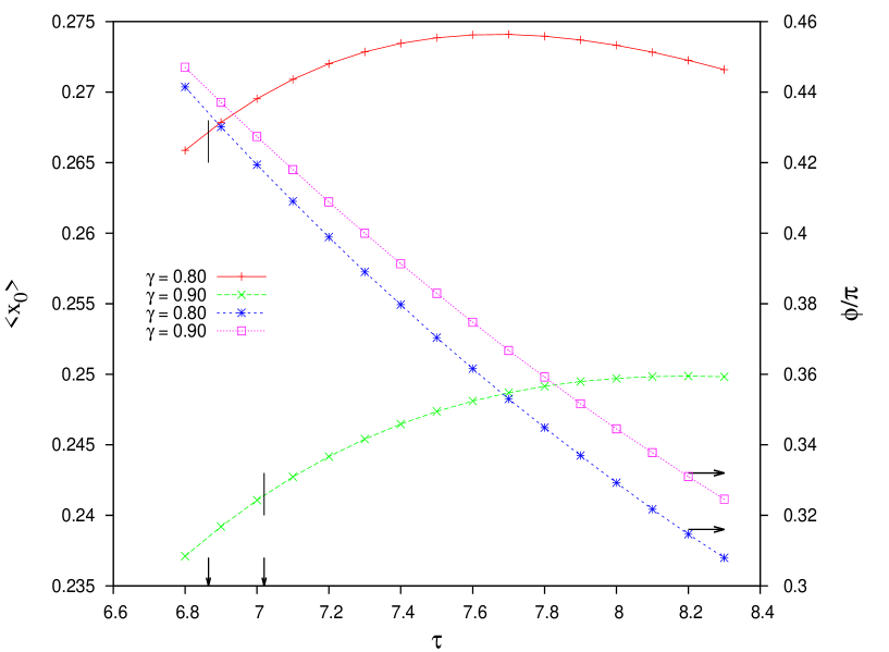
Figure 4: The figure shows the variation of the amplitude of the ensemble averaged hysteresis loop and the phase of the loop as a function of the driving period $\tau$. Note that the two graphs indicated by the horizontal arrows (y-axis label is towards the right hand side) signify the phase of the loop for the two $\gamma$ values as indicated. The right vertical arrow and the right vertical line on $<{x_{0}}>$ indicates the resonant period, $\tau_{0}$ = $7.02$ for $\gamma=0.90$ whereas the left vertical arrow and the left vertical line on $<{x_{0}}>$ is for $\gamma=0.80$ with $\tau_{0}$ = $6.865$.

Figure 2 is the main result of our paper. It shows the contrasting resonance behavior of a linear and a nonlinear system. Usual physical intuition often does not work in nonlinear systems. It is, therefore, hard to explain offhand why a simple pendulum behaves so differently from a harmonic oscillator as far as the resonance characteristics are concerned. We only try to provide a rough explanation using our numerical results.

The hysteresis loop area $\int Fdx$ depends on both the amplitude $<x_{0}>$ of the response trajectory $x(t)$ as well as the phase difference $\phi$ between $F(t)$ and $x(t)$. For intermediate as well as large damping $\gamma$, the phase difference $\phi$ decreases with increasing period $\tau$ of $F(t)$ for all $\gamma$ values. Also, the amplitude $<x_{0}>$ is smaller for larger $\gamma$ values for any period $\tau$ of the drive. These are understandable. However, as we can see from Figs. 3 and 4, the amplitude $<x_{0}>$ shows a nonmonotonic behavior, it peaks at some intermediate $\tau$ value. This is a peculiar feature in the present case of periodically driven underdamped sinusoidal (nonlinear) potential system.

II.1 Intermediate range of $\gamma$ values

This range refers to $0.165\leq\gamma\leq 0.38$, of $\gamma$ for $F_{0}=0.2$ and $0.099\leq\gamma<0.28$ for $F_{0}=0.1$. Both present similar features though we consider Fig. 3 for the former case only. Figure 3 shows both the amplitude $<x_{0}>$ and the phase lag $\phi$ together, for the two typical values of $\gamma$ equal to 0.24 and 0.32, for easy comparison. However, the inset of the figure has only the plot of phase lag as a function of the drive period $\tau$. The peculiar features to be noticed are that $<x_{0}>$ shows a peak in the lower $\tau$ range for both the $\gamma$ values. However, the peak corresponding to $\gamma=0.32$ occurs at a slightly lower value of $\tau$ than $\gamma=0.24$. Moreover, in the same small range of $\tau$ the phase lag $\phi$ is larger in the case of $\gamma=0.24$ than $\gamma=0.32$. On the other hand, in the larger range of $\tau$ the phase lag $\phi$ is larger for the larger $\gamma=0.32$. Thus in the larger range of $\tau$ the phase lag shows the usual behaviour. The small values of $\phi$ in this range shows that when the system is driven at a slow rate the system $x(t)$ follows the drive $F(t)$ closely. However, the same does not hold in the range of smaller $\tau$ (or larger frequency $\omega$) where inertia seems to play an important role.

In the larger frequency $\omega$ range it is difficult for the system $x(t)$ to follow the drive $F(t)$ and consequently the phase lag $\phi$ between them is large, $\phi$ close to $\frac{\pi}{2}$. Moreover, $x(t)$ seems to overshoot $F(t)$. That is, while $F(t)$ turns back from its maximum $x(t)$ continues on its way for a longer while, before it retraces its path back due to its inertia. And inertia is more effective at lower damping. However, at still larger frequencies the system again fails to respond to the field and the amplitude begins to decrease. With this plausible qualitative explanation of the peaking behaviour of $<x_{0}>$ as a function of $\tau$ it becomes easier to see why the resonance frequency $\overline{\omega_{0}}$ increases with decreasing amplitude $\overline{x_{0}}$.

As mentioned earlier, $\overline{\omega_{0}}$ corresponds to the drive frequency $\omega$ at which the mean power loss is maximum and $\overline{x_{0}}$ is the corresponding amplitude of $x(t)$. And, $F(t)$ being sinusoidal and $x(t)$ also being roughly sinusoidal, given an amplitude $<x_{0}>$ of $x(t)$ the power loss or the hysteresis $F(x)$ loop area becomes maximum when $\phi=\frac{\pi}{2}$. If $\phi$ is nearly $\frac{\pi}{2}$ it is the amplitude $<x_{0}>$ that determines the maximum of the hysteresis loss. Therefore in this case maximum of power loss occurs at a frequency close to where $<x_{0}>$ becomes maximum. From Fig. 3, one can, therefore, see that $\overline{\omega_{0}}$ is smaller for $\gamma=0.24$ than $\gamma=0.32$ with correspondingly larger $\overline{x_{0}}$ for $\gamma=0.24$ than $\gamma=0.32$. Thus, considering these two typical values of $\gamma$, in this intermediate range of $\gamma$, the curve $\overline{\omega_{0}}(\overline{x_{0}})$ should have the same qualitative nature as given in Fig. 2, that is, $\overline{\omega_{0}}$ decreases with increasing $\overline{x_{0}}$. However, the variation is not so sharp as in the large $\gamma$ case ($\gamma>0.38$ for $F_{0}=0.2$).

II.2 Large $\gamma$ regime

In this large damping ($\gamma>0.38$ for $F_{0}=0.2$ and $\gamma>0.28$ for $F_{0}=0.1$) regime naturally amplitudes $<x_{0}>$ of oscillation are relatively small compared to those in the smaller $\gamma$ regimes. It is also intuitively obvious that the response amplitude should decrease with increasing damping, for example, $<x_{0}>(\gamma=0.8)$ is greater than $<x_{0}>(\gamma=0.9)$. That the resonance frequency should also decrease with damping can be qualitatively explained again from the obtained variation of $<x_{0}>$ and $\phi$ with $\tau$ as in Fig. 4.

We choose two large values of $\gamma$ equal to 0.8 and 0.9 for illustration. Here, the phase lags $\phi$ are small ($\phi<\frac{\pi}{2}$) and $\phi$ is consistently smaller for $\gamma=0.8$ than $\gamma=0.9$ at any value of $\tau$. The effect of inertia gradually diminishes as $\gamma$ increases. The consequence of this can be seen from the diminishing sharpness of $<x_{0}>$ peaks with increasing $\gamma$. Also to be noticed from Fig. 4 is that in case of $\gamma=0.8$ the $<x_{0}>$ peak occurs at larger frequency (smaller $\tau$) than $\gamma=0.9$. The variation of $<x_{0}>$ is much smaller than the variation of $\phi$ in the plotted relevant region of $\tau$. The resonance peak occurs close to where the hysteresis loop area is the largest, that is where $\phi$ is large ($\approx\frac{\pi}{2}$), thus from the figure, close to small values of $\tau$ (but larger than in case of intermediate range of $\gamma$ considered earlier). Both $<x_{0}>$ and $\phi$ conspire together to maximize the hysteresis loop area to determine $\overline{\omega_{0}}$ and corresponding $\overline{x_{0}}$ at resonance. Fig. 4, thus helps in getting a plausible qualitative idea that at larger damping not only the resonance response amplitudes is smaller but the system becomes slower to respond too. The rapid rise of $\overline{\omega_{0}}$ with $\overline{x_{0}}$ with decreasing $\gamma$ is an outcome that does not seem unusual as $\gamma$ decreases $\overline{\omega_{0}}$ tends towards the natural frequency of oscillation $\omega_{1}$ at $\gamma=0$, Fig. 2.

II.3 Small $\gamma$ regime

For small $\gamma$ values, for example $0.06\leq\gamma<0.165$ for $F_{0}=0.2$, the explanation of the nature of the resonance curve $\overline{\omega_{0}}(\overline{x_{0}})$ has an entirely different origin. The resonance curve is disjoint from the earlier two regimes (in which the curves were contiguous). In this range of $\gamma$, the hysteresis loop area maximizes as a function of frequency in a region of frequency where there exists not one kind of particle trajectory but two for a given $\gamma$ and amplitude $F_{0}$ of $F(t)$ SaikiaX ; WandaX ; Decay . Of course, if the amplitude $F_{0}$ is large (say, $>0.25$), the trajectories become chaoticWanda1X . We consider only amplitudes $F_{0}$ that give nonchaotic trajectories.

Figure 5: The top panel represents an SA state with a small phase lag with respect to the forcing $F(t)$ with amplitude $F_{0}=0.2$. Notice that the amplitude $F_{0}$ in the top panel is magnified so that comparison with $x(t)$ can be visualised easily. The bottom panel represents the corresponding hysteresis loop.

Figure 6: The top panel represents an LA state with a larger phase lag with respect to the forcing $F(t)$ with amplitude $F_{0}=0.2$. Notice that the amplitude $F_{0}$ in the top panel is magnified so that comparison with $x(t)$ can be visualised easily. The bottom panel represents the corresponding hysteresis loop.

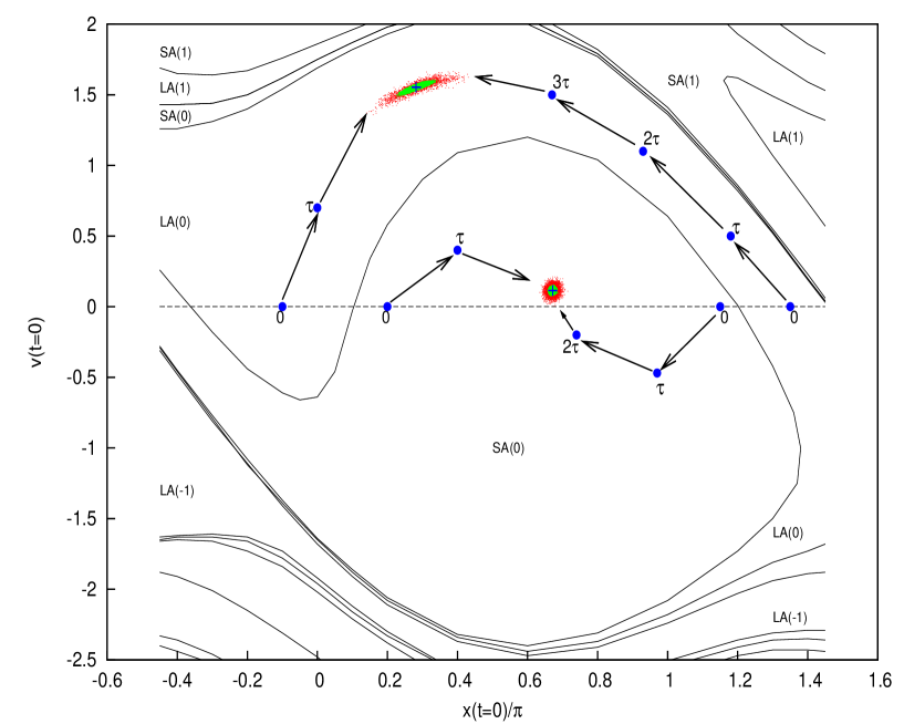
Figure 7: The basins of attraction of the LA and SA attractor in the absence (cross-mark) and presence of minute fluctuations is shown. The bracketed numbers on LA and SA indicate the well number of the periodic potential where the trajectory settles down in the LA attractor or the SA attractor. For this figure, $\gamma=0.12$, $\tau=8.0$ and $F_{0}=0.2$ and $V(x)=-\sin x$. The horizontal line in the middle is when the particles initially have velocity $v(t=0)=0$. Corresponding to this zero initial velocity, the LA attractors are the upper colored regions whereas the SA attractors are the lower colored regions. The green regions correspond to $T=0.0001$ and the red regions correspond to $T=0.001$.

These two states of trajectory have the status of distinct dynamical states having well defined basins of attraction in the ($x(0),v(0)$) space. One of the two states of trajectories has a comparatively small amplitude (SA) and has a small phase lag ($\phi<\frac{\pi}{3}$) with respect to the external drive $F(t)$ whereas the other state has a large amplitude (LA) and a large phase lag. Figures 5 and 6 show the SA and LA states with their respective mean hysteresis loops shown in the bottom panels of both the figures. To obtain the hysteresis loop, as explained earlier, the trajectory of the pendulum is averaged over the entire duration of the trajectory as $\overline{x}(F(t))$. The area bounded by the hysteresis loops corresponds to the energy dissipated to the surrounding medium. The basins of attraction of these two dynamical states with parameter values $\gamma=0.12$, $\tau=8.0$ and $F_{0}=0.2$ are shown earlier in SaikiaX . We reproduce an updated plot for explanation purposes in Fig. 7. In Fig. 7 we also show the stroboscopic plots in the $(x(0)-v(0))$ plane when the initial velocity of the particles at $t=0$ is $v(t=0)=0$ and in the absence and presence of minute thermal fluctuations. These stroboscopic plots appear in Fig. 7 as colored regions. In the absence of fluctuations, these stroboscopic regions reduce to a single point, corresponding to an attractor, as shown by the cross-mark. The upper stroboscopic plot corresponds to the LA attractor while the lower stroboscopic plot corresponds to the SA attractor. The basins of attraction shown in Fig. 7 have the usual physical significance. For example, if the initial position of the particle were to lie in the range of, say, $0.2\pi\leq x(0)\leq 1.1\pi$, then on evolving the system after initial transients have died out, the particle will home into the SA attractor and will remain in its initial well only. But on the other hand, suppose if the initial position of the particle were to lie in the range of, say, $-0.3\pi\leq x(0)\leq 0$, then the particle will oscillate with larger amplitude and get fixed to the LA attractor. The (transient) time evolutions towards the fixed centres of attractions have been shown schematically in Fig. 7 and marked by arrows. We note that the illustration given is when the initial velocity of the particle at any position within one period of the potential well is zero. This zero initial velocity is represented in Fig. 7 as a horizontal line.

Figure 8: Phase diagram in the $\omega$-$\gamma$ space denoting the regions of pure LA, pure SA, and coexistence region. Here, $F_{0}=0.2$.

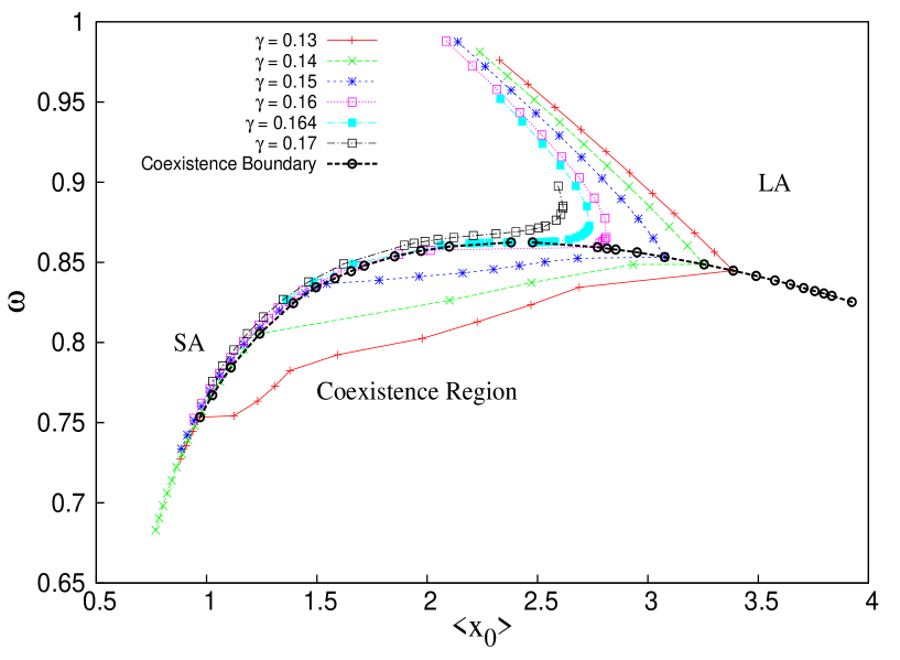
Figure 9: The figure shows the variation of the amplitudes of the LA state and the SA state as a function of the driving frequency $\omega$. The boundary line (dash-open circle line) separate the coexistence region from the regions where either SA state is present or LA state is present only. The amplitudes between the boundary line are calculated in the coexistence region for $\gamma=0.13$, $\gamma=0.14$ and $\gamma=0.15$.

For a given $\gamma$ the domain of the basins of attraction depends on the value of $\omega$, Fig. 8. For small $\omega$ (for example, for $\gamma=0.13,~{}\omega<0.74$) only SA states appear whereas for large $\omega$ (for the same $\gamma,~{}\omega>0.85$) the domain of the basins of attraction of SA states shrink to zero and only LA states appear and for the intermediate $\omega$ both states coexist. We choose initial velocity $v(0)=0$ always and hence the occurrence of LA or SA states depends on the initial position ($x(0)$) within a period of the sinusoidal potential. In the region of coexistence of the two states we choose two hundred initial positions lying in the range $\frac{-\pi}{2}<x(0)\leq\frac{3\pi}{2}$ at equal intervals in order to calculate the mean values that takes into account the presence of the two dynamical states in right proportions. At this point it should be noted that the hysteresis loop area corresponding to the LA states are larger compared to the area corresponding to the SA states and hence the need to consider all possible values of $x(0)$ in order to get the mean values of the hysteresis loop area and the mean amplitude $<x_{0}>$ of the trajectories.

For $\gamma>0.165$, in the intermediate range of $\gamma$ for $F_{0}=0.2$, there is only one kind of trajectory for all values of $\omega$ and initial positions $x(0)$, the mean amplitude $<{x_{0}}>$ varies continuously with the varation of $\omega$. It turns out that $\gamma\approx 0.164$ is the critical value of $\gamma$ above which there is no distinction between the LA and SA states. However, for $\gamma<0.164$, as mentioned earlier, for large value of $\omega$ we obtain only LA states but as $\omega$ is decreased some LA states corresponding to some initial positions $x(0)$ give way to SA states. The particular value of $\omega$, depending on the value of $\gamma$, at which SA states begin appearing also gives the largest hysteresis loop area and can be identified with $\overline{\omega_{0}}$ and the corresponding $<x_{0}>$ as the $\overline{x_{0}}$. The locus of these ($\overline{x_{0}},\overline{\omega_{0}}$) is shown in Fig. 9 by the right-hand side dash-open circle thick boundary line. This boundary line is the resonance line shown in Fig. 2 for $\gamma<0.165$. At $\gamma\approx 0.164$, $\overline{\omega_{0}}$ abruptly drops to a smaller value due to the sudden appearance of the SA states of trajectories (in place of some earlier LA trajectories) with mean hysteresis loop area of SA states being much smaller than LA states. The slopes of ($\overline{x_{0}},\overline{\omega_{0}}$) lines of Fig. 9 abruptly change indicating the beginning of the coexistence region of the two states.

II.4 A superficial analogy

Fig. 9 is quite instructive. Apart from the thick boundary line on the large $<x_{0}>$ side of the abscissa, we have an another thick boundary line on the small $<x_{0}>$ side. For smaller $<x_{0}>$ values we obtain only SA states of the pendulum. These two boundary lines, one separating the LA states from the coexistence region and the other separating the coexistence region from the purely SA region, meet at a point where the slope of the $(<x_{0}>,\omega)$ line is zero for $\gamma\approx 0.164$. This point is somewhat analogous to the critical point in the ($P-\rho$) diagram of the liquid-gas system. The two thick boundary lines thus enclose the region of coexistence of the two states and separate the LA states from the SA states of trajectories. We show in Fig. 9, for $\gamma=0.13$, $\gamma=0.14$ and $\gamma=0.15$, the mean amplitude of the trajectories when the particles are in the pure LA state, pure SA state and when the states coexists. For calculating the amplitude in the coexistence region, we ensemble average over all initial conditions taken and obtain the ensemble averaged hysteresis loop whereby the ensemble averaged amplitude can be calculated.

Though analogy of the SA and LA states of trajectories of the pendulum with the liquid-gas phase is quite superficial it is suggestively tempting to draw further analogy between the system of two dynamical states, LA and SA, of trajectories with the phases of the liquid-gas system. The frequency $\omega$ appears analogous to the pressure $P$, the friction coefficient $\gamma$ to the temperature $T$ and the amplitude $<x_{0}>$ of the trajectory to the density $\rho$ of the liquid. And finally the hysteresis loop area $\overline{A}(\omega,\gamma)$ seems analogous to the Gibbs free energy $g(P,T)$ of the liquid.

$$\begin{array}[]{c}\omega\longleftrightarrow P\\ \gamma\longleftrightarrow T\\ <x_{0}>\longleftrightarrow\rho\\ \overline{A}(\omega,\gamma)\longleftrightarrow g(P,T)\end{array}$$ (15)

However, these analogies are not exact but only superficial and cannot be stretched far.

III Concluding remarks

In this work we have investigated the dynamics of a driven damped simple pendulum or equivalently the motion of a particle in a sinusoidal potential in a medium that offers dissipation. Note that we have investigated the motion of the simple pendulum at the temperature $T=0$, that is, without considering the effect of thermal fluctuations. Also, we have kept the drive amplitude $F_{0}$ small so that the motion is nonchaotic.

In order to investigate the motion of a damped driven simple pendulum one needs to go much beyond the usual LCR circuit problem. In fact, no analytical solution has so far been found for this problem. The numerical solutions obtained, however, offer interesting insight. In the underdamped regime, in certain range of $\gamma$ and amplitude and frequency of the drive $F(t)$, two distinct solutions exist for the same periodic driving force $F(t)$. This leads to an entirely new relationship between the amplitude of motion with the resonance frequency of the simple pendulum having no relationship with the corresponding driven damped simple harmonic oscillator. That is, the resonance characteristics of the damped harmonic oscillator cannot be extrapolated to obtain the resonance characteristics of a damped simple pendulum.

References

- (1) A. Sommerfeld, Lectures on Theoretical Physics: Mechanics, Levant Books (Indian Reprint), Kolkata (2003).
- (2) C. Kittel, W. D. Knight, and M. A. Ruderman, Berkeley Physics Course - Volume I, Mechanics McGraw-Hill Book Company, Inc., New York (1962).
- (3) J. B. Marion, Classical Dynamics of Particles and Systems, Second Edition, Academic Press Inc., Orlando, 1970.
- (4) R. B. Kidd, and S. L. Fogg, The Physics Teacher 40, 81(2002).
- (5) R. R. Parwani, Eur. J. Phys. 25, 37(2004).
- (6) F. M. S. Lima, and P. Arun, Am. J. Phys. 74, 892(2006).
- (7) K. Johannessen, Eur. J. Phys. 32, 407(2011).
- (8) A. Beléndez, E. Arribas, A. Márquez, M.Ortaño, and S. Gallego, Eur. J. Phys. 32, 1303(2011).
- (9) A. H. Salas, https://www.researchgate.net/Publication/290946080 (January 2016).
- (10) Handbook of Mathematical Functions, Edited by M. Abramowitz, and I. A. Stegun, Dover Publications, Inc, New York, 1965.
- (11) D. Kleppner, and R. Kolenkow, An Introduction to Mechanics, Tata McGraw Hill, Special Indian Edition, New Delhi, 2007.
- (12) K. Johannesen, Eur. J. Phys. 35, 035014(2014).
- (13) S. Saikia, A. M. Jayannavar, and M. C. Mahato, Phys. Rev. E 83, 061121 (2011).
- (14) W. L. Reenbohn and M. C. Mahato, Phys. Rev. E 88, 032143 (2013).
- (15) D. Kharkongor, W. L. Reenbohn, and M. C. Mahato, Phys. Rev. E 94, 022148 (2016).
- (16) W. L. Reenbohn, and M. C. Mahato, Phys. Rev. E 91, 052151 (2015).