Heterogeneous continuous time random walks

Abstract

We introduce a heterogeneous continuous time random walk (HCTRW) model as a versatile analytical formalism for studying and modeling diffusion processes in heterogeneous structures, such as porous or disordered media, multiscale or crowded environments, weighted graphs or networks. We derive the exact form of the propagator and investigate the effects of spatio-temporal heterogeneities onto the diffusive dynamics via the spectral properties of the generalized transition matrix. In particular, we show how the distribution of first passage times changes due to local and global heterogeneities of the medium. The HCTRW formalism offers a unified mathematical language to address various diffusion-reaction problems, with numerous applications in material sciences, physics, chemistry, biology, and social sciences.

I Introduction

Understanding transport phenomena in multiscale porous media and crowded environments is of paramount importance in material sciences (e.g. hardening of concretes or degradation of monuments caused by salts penetration into stones), in petrol industry (oil extraction from sedimentary rocks), in agriculture (moisture propagation in soils), in ecology (contamination of underground water reservoirs and streams), in chemistry (diffusion of reactants towards porous catalysts), in biology (transport inside cells and organs, such as lungs, kidney, placenta), to name but a few Bouchaud ; Sahimi1993 ; Coppens99 ; Kirchner00 ; Berkowitz2000 ; Song00 ; Berkowitz02 ; Scher02 ; Plassais05 ; Gallos07 ; Dentz08 ; Zoia09 ; Scher10 ; Berkowitz10 ; Bressloff2013 ; Metzler2014 ; Serov16 . In spite of a significant progress in imaging techniques and computational tools over the last decade, accurate modeling of these processes is still restricted to a relatively narrow range of time and length scales. At the same time, the multiscale structure of porous media has a critical impact onto the transport properties Sahimi2012 ; Levitz2002 ; Levitz2012 . For instance, concretes exhibit pore sizes from few nanometers in the cement paste to few centimeters (or larger) that greatly impacts water diffusion, the consequent cement hydration and, ultimately, the mechanical properties of the material. Bridging theories and simulations on different scales has become at the heart of modern approaches to such multiscale phenomena. In particular, one aims at coarse-graining an immense amount of microscopic geometrical information about the medium from high-resolution imaging, and revealing the structural features that are the most relevant for a macroscopic description of the transport processes.

In this light, continuous time random walks (CTRWs), introduced by Montroll and Weiss montroll1965 ; Montroll1969 ; Montroll1973 , have been often evoked as an important model of diffusive transport in disordered and porous media Metzler1998 ; Metzler04 ; Barkai2008 ; Sahimi2012 ; Kang11 ; Fouxon2016 ; Amitai2017 . In this model, a diffusing particle spends a random time at a region of space (e.g., a pore) or at a site of a lattice before jumping to another region or site. The waiting event reflects either energetic trapping of the walker in a local minimum of the potential energy landscape, or a geometric trapping in a pore separated from other pores by narrow channels (Fig. 1) Bouchaud ; Scher1973 ; Levitz2002 ; Levitz2012 ; Kenkre1973 ; Bouten1986 . This model is intrinsically homogeneous, as all sites have the same waiting time distribution $\psi(t)$. In practice, however, pores and channels have a broad distribution of sizes and shapes, as well as the local minima of the potential energy landscape are broadly distributed. An extension of the conventional approach by considering a site-dependent waiting time distribution, $\psi_{x}(t)$, may capture the heterogeneity of the minima or pore shapes but ignores heterogeneities in mutual minima arrangements or in inter-pore connections. For this reason, we propose a more general approach that we call heterogeneous continuous time random walk (HCTRW). In this approach, a random walker moves on a graph, jumping from a site $x$ to a site $x^{\prime}$ with the probability $Q_{xx^{\prime}}$. The graph can be either a natural representation of the studied system (e.g., electric, transportation, internet or social network), or constructed as a coarse-grained representation of a potential energy landscape or a porous medium (Fig. 1). Graphs can also serve as discrete approximations (meshes) to Euclidean domains and manifolds. The travel (or exchange) time $\mathcal{T}_{xx^{\prime}}$ needed to move from $x$ to $x^{\prime}$ is a random variable drawn from the probability density $\psi_{xx^{\prime}}(t)$, which depends on both sites $x$ and $x^{\prime}$. In this paper, we only consider the Markovian case with independent jumps on connected graphs.

The paper is organized as follows. In Sec. II we introduce the HCTRW framework and derive the exact formula for the Laplace-transformed propagator. We show that the dynamics of HCTRW is fully determined by the spectral properties of the generalized transition matrix that couples temporal and spatial heterogeneities. Using perturbation theory we establish the long-time asymptotic behavior of the propagator for both finite and infinite mean travel times. In Sec. III, we show the relation of the HCTRW formalism to multi-state switching models. We also discuss a natural inclusion of boundary conditions into the model and the consequent possibility to assess various first passage quantities and reaction kinetics in a unified way. In particular, the peculiar effects of spatio-temporal heterogeneities onto the first passage time (FPT) distribution are presented. An explicit solution for the HCTRW propagator on $m$-circular graphs and some technical derivations are reported in Appendices.

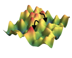
Figure 1: (Left). A complex dynamics in a disordered potential energy landscape can be approximated as HCTRW between local minima (defining the sites of the coarse-graining graph) with random exchange times ${{\mathcal{T}}}_{xx^{\prime}}$ between neighboring sites $x$ and $x^{\prime}$ drawn from an exponential probability density $\psi_{xx^{\prime}}(t)$ with the mean time $\tau_{xx^{\prime}}\propto\exp(U_{xx^{\prime}}/kT)$, where $U_{xx^{\prime}}$ is the energetic barrier between two minima and $kT$ is the thermal energy. (Right). Diffusion of a particle (shown by a hexagon) inside a porous medium (white space with gray obstacles) can be approximated as HCTRW between pores (defining the sites of the coarse-graining graph) with random travel times ${{\mathcal{T}}}_{xx^{\prime}}$ between neighboring sites $x$ and $x^{\prime}$ drawn from an exit time (or travel time) probability density $\psi_{xx^{\prime}}(t)$ determined by the shape of the pore at $x$ and its connections to neighboring pores $x^{\prime}$.

II General formalism

II.1 Propagator

We derive the general formula for the propagator $P_{x_{0}x}(t)$ of the HCTRW on a graph. Here we adapt the matrix notation, writing $x_{0}$ and $x$ as subscripts. The propagator $P_{x_{0}x}(t)$ is the probability to find a walker at a site $x$ at time $t$ if it started from a site $x_{0}$ at time $0$. This probability can be written as

$$P_{x_{0}x}(t)=\sum_{n=0}^{\infty}P_{x_{0}x}^{(n)}(t),$$ (1)

where $P_{x_{0}x}^{(n)}(t)$ is the probability to find the random walker, started from $x_{0}$, at $x$ at time $t$ after $n$ independent jumps. Note that the order of starting and ending points is important since we consider a general, not necessarily symmetric, transition matrix $Q$. Each component $P_{x_{0}x}^{(n)}(t)$ can be represented as

$$P_{x_{0}x}^{(n)}(t)=\int_{0}^{t}R_{x_{0}x}^{(n)}(t^{\prime})\Psi_{x}(t-t^{\prime})dt^{\prime},$$ (2)

where $\Psi_{x}(t-t^{\prime})$ is the probability of staying at site $x$ during time $t-t^{\prime}$ and $R_{x_{0}x}^{(n)}(t^{\prime})$ is the probability density to reach $x$ from $x_{0}$ at time $t^{\prime}$ at the $n^{th}$ step, which due to the Markovian property is

$$R_{x_{0}x}^{(n)}(t)=\int_{0}^{t}dt^{\prime}\sum_{x^{\prime}}R_{x_{0}x^{\prime}}^{(n)}(t^{\prime})Q_{x^{\prime}x}(t-t^{\prime}),$$ (3)

where $Q_{x^{\prime}x}(t)$ is the joint transition probability density:

$$Q_{x^{\prime}x}(t)=Q_{x^{\prime}x}\psi_{x^{\prime}x}(t).$$ (4)

The structural heterogeneities of the graph, represented by the transition matrix $Q$ spitzer ; Kehr1987 ; Weiss94 ; mugnolo2008 ; Sokolov2006 ; Angstmann13 , are now coupled, via the generalized transition matrix $Q(t)$, to dynamical heterogeneities represented by the densities $\psi_{x^{\prime}x}(t)$. In contrast to the Montroll-Weiss formula for ordinary CTRW with a continuous jump distribution, there is no Fourier transform in Eq. (2) because the probability $P^{(n)}_{x^{\prime}x}(t-t^{\prime})$ is written for a discrete graph (see Appendix A.1). Applying the Laplace transform to Eq. (2) and using its linearity and convolution property, one gets

$$\tilde{R}_{x_{0}x}^{(n)}(s)=\sum_{x^{\prime}}\tilde{R}_{x_{0}x^{\prime}}^{(n)}(s)[\tilde{Q}(s)]_{x^{\prime}x},$$ (5)

where $\tilde{Q}(s)$ is the Laplace transform of $Q(t)$

$$\tilde{Q}_{x^{\prime}x}(s)=Q_{x^{\prime}x}\tilde{\psi}_{x^{\prime}x}(s),$$ (6)

with the Laplace transform of quantities denoted with the tilde above them, e.g., $\tilde{\psi}_{x^{\prime}x}(s)=\int_{0}^{\infty}\psi_{x^{\prime}x}(t)e^{-st}dt$. With this notation, we can write Eq. (5) in a compact form

$$\tilde{R}^{(n)}_{x_{0}x}(s)=[\tilde{Q}(s)^{n}]_{x_{0}x}.$$ (7)

Hence we get the Laplace transform of the propagator $\tilde{P}_{x_{0}x}(s)$ using Eq. (1):

$$\tilde{P}_{x_{0}x}(s)=[(I-\tilde{Q}(s))^{-1}]_{x_{0}x}\,\tilde{\Psi}_{x}(s),$$ (8)

where the geometric series formula was applied to the sum of powers $(\tilde{Q}(s))^{n}$ given that $\|\tilde{Q}\|\leq 1$ (see Appendix A.2). Writing

$$\tilde{\Psi}_{x}(s)=\frac{1-\sum_{x^{\prime}}\tilde{Q}_{xx^{\prime}}(s)}{s},$$ (9)

the final expression of the propagator of HCTRW in the Laplace domain is

$$\tilde{P}_{x_{0}x}(s)=\frac{1-\sum_{x^{\prime}}\tilde{Q}_{xx^{\prime}}(s)}{s}[(I-\tilde{Q}(s))^{-1}]_{x_{0}x}.$$ (10)

This is one of the main results of the paper. Note that the propagator determines all the moments of the position of the walker, including the mean squared displacement.

The inverse Laplace transform is then needed to get the propagator in time domain. When the exchange times are drawn from exponential distributions, $\tilde{\psi}_{xx^{\prime}}(s)=(1+s\tau_{xx^{\prime}})^{-1}$, $\tilde{P}_{x_{0}x}(s)$ in Eq. (10) is a ratio of two polynomials of $s$, whereas $P_{x_{0}x}(t)$ gets the usual form of a sum of exponentially decaying functions. In this practically relevant case, one needs to find the poles of $\tilde{P}_{x_{0}x}(s)$, i.e., the zeros of the equation ${\textrm{det}}(I-\tilde{Q}(s))=0$. The Gerschgorin theorem determines the radius of a disk in the complex plane, in which the poles are located, and hence speeds up their numerical calculation Carstensen1989 . In the homogeneous case, $\tilde{\psi}_{xx^{\prime}}(s)=\tilde{\psi}(s)=(1+s\tau)^{-1}$, the problem is reduced to computing the eigenvalues $\lambda_{k}^{0}$ of the matrix $H_{0}=I-Q$ and then finding $s$ at which $\tilde{\psi}(s)=1/(1-\lambda_{k}^{0})$. One gets thus the poles $s_{k}=-\lambda_{k}^{0}/\tau$, as expected. In general, however, spatio-temporal heterogeneities in $\tilde{\psi}_{xx^{\prime}}(s)$ can significantly alter the above relation between the dynamical properties of the HCTRW (determined by the poles $s_{k}$) and the spectral properties of the stochastic matrix (the eigenvalues $\lambda_{k}^{0}$). Moreover, if some $\tilde{\psi}_{xx^{\prime}}(s)$ are non-analytic, the Laplace-transformed propagator can also be non-analytic. As a consequence, $P_{x_{0}x}(t)$ may not be expressed as a sum of exponentials, exhibiting a slower approach to the steady-state limit (see below).

II.2 Spectral analysis and the long-time behavior

In general, the matrix $H(s)=I-\tilde{Q}(s)$ is real but not symmetric so that its complex-valued eigenvalues form complex conjugate pairs Trefethen . For each $s$, we denote $u_{k},v_{k}$ the left and right eigenvectors of $H(s)$, associated with the same eigenvalue $\lambda_{k}$:

$$u_{k}\,H(s)={\lambda_{k}}\,u_{k},\qquad H(s)\,v_{k}=\lambda_{k}\,v_{k}.$$ (11)

The left eigenvectors of $H(s)$ are just the transpose of the right eigenvectors of the transposed matrix $H(s)^{\dagger}$. One gets thus the spectral representation of Eq. (10)

$$\tilde{P}_{x_{0}x}(s)=\frac{1-\sum_{x^{\prime}}\tilde{Q}_{xx^{\prime}}(s)}{s}\sum_{k\geq 0}\frac{v_{k}(x_{0})\,u_{k}(x)}{\lambda_{k}},$$ (12)

where we used bi-orthogonality: $(u_{j}\cdot v_{k})=\delta_{j,k}$. Since $u_{k}$ is a left row-vector, we do not write the transpose symbol $\dagger$ for $u_{k}$. Although the explicit dependence on $x_{0}$ and $x$ is factored out in Eq. (12), this representation remains rather formal, since $u_{k},v_{k}$ and $\lambda_{k}$ depend on $s$ in a highly non-trivial way. However it shows that the spectral properties of the generalized transition matrix $\tilde{Q}(s)$ fully determine the propagator of HCTRW. In some particular cases, the eigenvalues and eigenvectors of the matrix $H$ can be found explicitly, allowing one to derive an explicit form of the propagator in time domain, as illustrated in Appendix B for $m$-circular graphs. In general, however, the time dependence of the propagator over the whole range of times is difficult to grasp, and one focuses on long-time asymptotic behavior.

The long-time behavior of HCTRW is determined by $\tilde{P}_{x_{0}x}(s)$ at small $s$. Here we distinguish two cases: (i) when all mean travel times $\langle{{\mathcal{T}}}_{xx^{\prime}}\rangle$ are finite, and (ii) when at least one of the mean travel times is infinite.

In the former case, one gets the expansion

$$\tilde{\psi}_{xx^{\prime}}(s)=1-s\langle\mathcal{T}_{xx^{\prime}}\rangle+o(s).$$ (13)

Introducing a matrix $T$ with elements

$$T_{xx^{\prime}}=Q_{xx^{\prime}}\langle\mathcal{T}_{xx^{\prime}}\rangle,$$ (14)

one gets $H(s)\approx I-Q+sT+o(s)$ so that the Laplace transform of the propagator can be approximated as

$$\tilde{P}_{x_{0}x}(s)\simeq t_{x}\bigg{[}(I-Q+sT)^{-1}\bigg{]}_{x_{0}x},$$ (15)

where

$$t_{x}=\sum_{x^{\prime}}T_{xx^{\prime}}.$$ (16)

The normalization of the propagator is preserved even in this approximate form (see Appendix A.3).

Using the standard perturbation analysis at small $s$ Kato ; Sternheim , we substitute the expansions

$$\lambda_{k} = \lambda_{k}^{0}+s\lambda_{k}^{1}+o(s),$$ (17a)

$$u_{k} = u_{k}^{0}+su_{k}^{1}+o(s),$$ (17b)

$$v_{k} = v_{k}^{0}+sv_{k}^{1}+o(s)$$ (17c)

into Eq. (11) to get in the zeroth and first order in $s$:

$$u_{k}^{0}H_{0}=\lambda_{k}^{0}u_{k}^{0},\quad H_{0}v_{k}^{0}=\lambda_{k}^{0}v_{k}^{0},$$ (18a)

$$u_{k}^{0}H_{0}+u_{k}^{0}T=\lambda_{k}^{0}u_{k}^{0}+\lambda_{k}^{1}u_{k}^{0},$$ (18b)

$$H_{0}v_{k}^{0}+Tv_{k}^{0}=\lambda_{k}^{0}v_{k}^{0}+\lambda_{k}^{1}v_{k}^{0}.$$ (18c)

Multiplying the second equation by $u_{k}^{0}$, we get

$$\lambda_{k}^{1}=(u_{k}^{0}Tv_{k}^{0}).$$ (19)

Then to the first order Eq. (12) becomes:

$$\tilde{P}_{x_{0}x}(s)\simeq t_{x}\sum_{k\geq 0}\frac{v_{k}^{0}(x_{0})\,u_{k}^{0}(x)}{\lambda_{k}^{0}+s\lambda_{k}^{1}}.$$ (20)

Given that $\lambda_{0}^{0}=0$ and $v_{0}^{0}=1/\sqrt{N}$ due to the normalization of the transition matrix $Q$, where $N$ is the number of vertices in the graph, it is convenient to isolate the term with $k=0$:

$$\tilde{P}_{x_{0}x}(s)\simeq\frac{p^{\rm st}_{x}}{s}+t_{x}\sum_{k>0}\frac{v_{k}^{0}(x_{0})\,u_{k}^{0}(x)}{\lambda_{k}^{0}+s\lambda_{k}^{1}},$$ (21)

where

$$p^{\rm st}_{x}=\frac{t_{x}\pi_{x}}{\sum_{x^{\prime}}t_{x^{\prime}}\pi_{x^{\prime}}}$$ (22)

is the steady-state (stationary) distribution, with $\pi_{x}$ being the steady-state distribution of the ordinary random walk on the graph, governed by the transition matrix $Q$: $\pi Q=\pi$ (see Appendix A.4).

The ratio $-\lambda_{k}^{0}/\lambda_{k}^{1}$ in Eq. (21) is the pole of the approximate Laplace-transformed propagator and thus an approximation of the real pole $s_{k}$. This approximation can only be valid for poles with the small absolute value $|s_{k}|$. Denoting $\tau_{m}=\max\limits_{k>0}\{\lambda_{k}^{1}/\lambda_{k}^{0}\}=\lambda_{k_{m}}^{1}/\lambda_{k_{m}}^{0}$ (for some index $k_{m}$) as the largest time scale, we get the long-time exponential approach to the steady-state distribution:

$$P_{x_{0}x}(t)\simeq p^{\rm st}_{x}+t_{x}\frac{v_{k_{m}}^{0}(x_{0})\,u_{k_{m}}^{0}(x)}{\lambda_{k_{m}}^{1}}\,e^{-t/\tau_{m}}.$$ (23)

The above analysis is not applicable when at least one mean travel time is infinite. We sketch the main steps of the asymptotic analysis for the particular situation when all probability densities $\psi_{xx^{\prime}}(t)$ exhibit heavy tails with the same scaling exponent $0<\alpha<1$: $\psi_{xx^{\prime}}(t)\propto t^{-1-\alpha}$ or, equivalently,

$$\tilde{\psi}_{xx^{\prime}}(s)=1-s^{\alpha}\tau_{xx^{\prime}}^{\alpha}+o(s^{\alpha}),$$ (24)

with possibly different time scales $\tau_{xx^{\prime}}$. The propagator is then approximated as

$$\tilde{P}_{x_{0}x}(s)\simeq s^{\alpha-1}t_{x}\bigg{[}(I-Q+s^{\alpha}T)^{-1}\bigg{]}_{x_{0}x},$$ (25)

with the matrix $T$ being still defined by Eq. (14), in which $\langle{{\mathcal{T}}}_{xx^{\prime}}\rangle$ are replaced by $\tau_{xx^{\prime}}^{\alpha}$, and $t_{x}$ is defined by Eq. (16).

For small $s$, one can apply the same perturbation theory, in which $s$ is replaced by $s^{\alpha}$, to get

$$\tilde{P}_{x_{0}x}(s)\simeq s^{\alpha-1}t_{x}\sum_{k\geq 0}\frac{v_{k}^{0}(x_{0})\,u_{k}^{0}(x)}{\lambda_{k}^{0}+s^{\alpha}\lambda_{k}^{1}}.$$ (26)

The formal inversion of the Laplace transform yields the long-time asymptotic approach to the steady-state

$$P_{x_{0}x}(t) \simeq p^{\rm st}_{x}+t_{x}\frac{v_{k_{m}}^{0}(x_{0})\,u_{k_{m}}^{0}(x)}{\lambda_{k_{m}}^{1}}E_{\alpha}(-t^{\alpha}/\tau_{m}),$$ (27)

where $E_{\alpha}(z)$ is the Mittag-Leffler function. Since the Mittag-Leffler function exhibits a slow, power law decay, $E_{\alpha}(-z)\simeq z^{-1}/\Gamma(1-\alpha)$ as $z\to\infty$, the major difference with the former case of finite mean travel times is a much slower approach to the steady-state limit, which is caused by long traps.

III Discussion

The HCTRW model naturally describes multi-state systems, for which the states are represented by nodes and the probability densities $\psi_{xx^{\prime}}(t)$ characterize the inverse of random exchange rates. The simplest example is a two-state system, which switches randomly between two states $1$ and $2$ after random times ${{\mathcal{T}}}_{12}$ and ${{\mathcal{T}}}_{21}$ drawn from the probability densities $\psi_{12}(t)$ and $\psi_{21}(t)$. In this case, $Q=\biggl{(}\begin{array}[]{c c}0&1\\ 1&0\\ \end{array}\biggr{)}$, and the Laplace-transformed propagator reads as

$$\tilde{P}(s)=\frac{1}{s(1-\tilde{\psi}_{12}(s)\tilde{\psi}_{21}(s))}$$

$$\times\left(\begin{array}[]{c c}1-\tilde{\psi}_{12}(s)&(1-\tilde{\psi}_{21}(s))\tilde{\psi}_{12}(s)\\ (1-\tilde{\psi}_{12}(s))\tilde{\psi}_{21}(s)&1-\tilde{\psi}_{21}(s)\\ \end{array}\right),$$ (30)

where $\tilde{P}(s)$ is a $2\times 2$ matrix notation for $\tilde{P}_{x_{0}x}(s)$. In particular, the non-Markovian dynamics of such a simple system was established when $\psi_{xx^{\prime}}(t)$ are not exponential densities Boguna2000 . The HCTRW formalism naturally extends this analysis to a multi-state system, which randomly switches between $N$ different states. More generally, the HCTRW framework can be related to the theory of renewal processes WilmerLevin , to random walks in random environments Hughes ; Zeitouni2002 , and to persistent CTRW Jaume2017 .

The matrix $H=I-\tilde{Q}(s)$ can be seen as a normalized form of a weighted discrete Laplacian on a graph, which is also related to the model of random resistor networks Mieghem . Since the generalized transition matrix $\tilde{Q}(s)$ couples the structure of the graph (the matrix $Q$) to the spatio-temporal dynamics of the walker on that graph (the densities $\psi_{xx^{\prime}}(t)$), it is natural to distinguish the effects of both aspects. In particular, one can investigate how the spectral properties of the matrix $\tilde{Q}(s)$ are affected by structural (or geometric) and spatio-temporal (or distributional) perturbations. In the former case, one changes the structure of the graph (e.g., by adding, removing, or modifying some links). In the latter case, the graph is kept fixed but the densities $\phi_{xx^{\prime}}(t)$ are modified. Analytical estimates for the propagator under spatio-temporal perturbations can be derived by using the time-dependent perturbation theory Griffiths , and approximations for the smallest eigenvalue Zou2009 ; Hunter1986 .

III.1 Absorbing boundary, bulk reactions, and first passage phenomena

In contrast to continuous-space problems, one can naturally accommodate boundary conditions through the stochastic matrix $Q$, with no change to the HCTRW formalism. In fact, a reflecting boundary is intrinsically implemented by the mere fact of a finite-size matrix $Q$. An absorbing boundary or a target can be implemented by adding a “sink site” $x^{*}$ to the graph, such that $Q_{x^{*}x^{*}}=1$, i.e., any particle that comes to $x^{*}$ remains trapped at this site. The geometric structure of the absorbing boundary (or the target) is captured through the elements of the matrix $Q_{xx^{*}}$, i.e., the probabilities of arriving at the sink site from other sites of the graph. The propagator $P_{x_{0}x}(t)$ is then interpreted as the probability for a walker started at $x_{0}$ to be at a site $x$ at time $t$ without being absorbed. In turn, $P_{x_{0}x^{*}}(t)$ is the probability of being absorbed by time $t$, whereas $S_{x_{0}}(t)=1-P_{x_{0}x^{*}}(t)$ is the survival probability. As a consequence, $P_{x_{0}x^{*}}(t)$ can be interpreted as the cumulative probability distribution of the first passage time (FPT) to the sink site (or to the absorbing boundary), whereas $\rho_{x_{0}}(t)=\partial P_{x_{0}x^{*}}(t)/\partial t$ is the probability density of this FPT. The mean FPT is simply $\tilde{P}_{x_{0}x^{*}}(0)$, and other moments of the FPT are expressed as derivatives of the Laplace-transformed propagator $\tilde{P}_{x_{0}x^{*}}(s)$ at $s=0$. One can also easily treat partially absorbing boundaries Collins49 ; Sano79 ; Sapoval94 ; Grebenkov03 ; Grebenkov06 ; Grebenkov07 ; Singer08 ; Grebenkov10b ; Rojo12 by allowing nonzero leakage probability from the sink site $x^{*}$.

If a particle can disappear or loose its activity during diffusion, FPT problems for such “mortal” walkers Abad10 ; Abad12 ; Abad13 ; Yuste13 ; Abad15 ; Meerson15a ; Meerson15b ; Grebenkov17 can be treated by introducing two sink sites, $x^{*}_{1}$ and $x^{*}_{2}$, that represent an absorbing boundary and a reactive bulk. Using the exchange time distributions $\psi_{xx^{*}_{2}}(t)$ depending on $x$, one can model space-dependent bulk reaction rates. Note also that $P_{x_{0}x^{*}_{1}}(\infty)$ is the splitting probability, i.e., the probability of the arrival on $x^{*}_{1}$ before arriving on $x^{*}_{2}$ (i.e., the arrival to the target before dying or loosing activity). If there are many sink sites $x^{*}_{1},\ldots,x^{*}_{k}$, $P_{x_{0}x^{*}_{i}}(\infty)$ are the hitting probabilities (a discrete analog of the harmonic measure).

All these conventional concepts of first passage phenomena Redner2002 are accessible through the mathematical formalism of HCTRW which plays thus a unifying role. The main advantage of this approach is the reduction of the sophisticated dynamics in heterogeneous media to the spectral properties of the governing matrix $\tilde{Q}(s)$ which generalizes the stochastic matrix $Q$. In the same way as the structural features of the medium that are relevant for simple random walks were captured through the spectral properties of the transition matrix $Q$ Lin13 , the spatio-temporal heterogeneities of the medium are captured by the spectral properties of the generalized transition matrix $\tilde{Q}(s)$.

III.2 Effects of spatio-temporal heterogeneities on first passage times

If one is primarily interested in the impact of spatio-temporal heterogeneities onto the diffusive dynamics, one can choose the simplest geometric setting, a discretized interval, represented by a graph with $N=100$ sites. We consider a symmetric HCTRW on this graph, with equal probabilities to move to the left and to the right. The nodes $x^{*}=1$ and $x=100$ are respectively absorbing and reflecting. This fixes the transition matrix $Q$ as follows: $Q_{xx^{\prime}}=\frac{1}{2}\delta_{x,x^{\prime}-1}+\frac{1}{2}\delta_{x,x^{\prime}+1}$ for $1<x<N$; $Q_{1x^{\prime}}=\delta_{1,x^{\prime}}$; and $Q_{Nx^{\prime}}=\frac{1}{2}\delta_{N,x^{\prime}-1}+\frac{1}{2}\delta_{N,x^{\prime}}$. In turn, the temporal aspects of diffusion, represented by travel time densities $\psi_{xx^{\prime}}(t)$, will be explored. Note that the results do not depend on the choice of the density $\psi_{x^{*}x^{*}}(t)$ at the sink site (see Appendix A.5).

Although various diffusive characteristics are available, we focus on the probability density $\rho_{x_{0}}(t)$ of the FPT. For each considered example, we compute this density by using the Talbot algorithm Talbot79 for a numerical inversion of the Laplace transform of $s\tilde{P}_{x_{0}x^{*}}(s)$ (with $x^{*}=1$). To validate this inversion procedure, we compare $\rho_{x_{0}}(t)$ in the homogeneous case with $\tilde{\psi}_{xx^{\prime}}(s)=(1+s\tau)^{-1}$, to the known solution of the FPT probability density for Brownian motion on the unit interval $(0,1)$ with absorbing (resp. reflecting) endpoint at $0$ (resp., at $1$):

$$\rho_{z_{0}}^{\rm BM}(t)=\pi D\sum\limits_{n=0}^{\infty}(n+1/2)\sin(\pi(n+1/2)z_{0})e^{-\pi^{2}(n+\frac{1}{2})^{2}Dt},$$ (31)

where $D$ is the diffusion coefficient, and $z_{0}=x_{0}/N$. Setting $D=a^{2}/(2\tau)$ with $a=1/N$ being the inter-site distance, one expects that the homogeneous diffusion on this graph is a discrete approximation of Brownian motion so that $\rho_{x_{0}}(t)$ and $\rho_{x_{0}/N}^{\rm BM}(t)$ are close to each other. One can see an excellent agreement between two functions (shown by solid line and crosses) in Fig. 2, except at short times at which small deviations can be attributed to the discretization of the interval by $N$ points. After this validation, we will reveal the impact of spatio-temporal heterogeneities by comparing all results to the homogeneous case, with $\tilde{\psi}_{xx^{\prime}}(s)=(1+s\tau)^{-1}$.

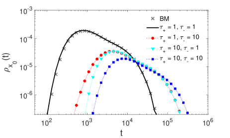
Figure 2: FPT probability density $\rho_{x_{0}}(t)$ for symmetric HCTRW on a discrete interval with $N=100$ sites, the absorbing endpoint at $x^{*}=1$, and the reflecting endpoint at $x=100$. We set $x_{0}=50$ and $\tilde{\psi}_{xx^{\prime}}(s)=(1+s\tau_{xx^{\prime}})^{-1}$, with $\tau_{xx^{\prime}}=\tau_{+}\delta_{x,x^{\prime}-1}+\tau_{-}\delta_{x,x^{\prime}+1}$. Gray crosses show the density $\rho_{z_{0}}^{\rm BM}(t)$ for Brownian motion on the unit interval, with $D=1/(2N^{2})$ and $z_{0}=x_{0}/N$.

First, we illustrate the effect of nonsymmetric travel times. For this purpose, we set $\tilde{\psi}_{xx^{\prime}}(s)=(1+s\tau_{xx^{\prime}})^{-1}$ with $\tau_{xx^{\prime}}=\tau_{+}\delta_{x,x^{\prime}-1}+\tau_{-}\delta_{x,x^{\prime}+1}$. In other words, we consider a random walker jumping with exponentially distributed travel times but the mean time to jump to the left, $\tau_{-}$, is different from the mean time to jump to the right, $\tau_{+}$. This difference may originate, e.g., from a potential inside channels connecting neighboring pores. We emphasize that the probabilities of jumping to the left and to the right remain equal. Figure 2 compares four cases: (a) $\tau_{+}=\tau_{-}=1$; (b) $\tau_{+}=10$, $\tau_{-}=1$; (c) $\tau_{+}=1$, $\tau_{-}=10$; and (d) $\tau_{+}=\tau_{-}=10$. As expected, the cases (a) and (d) yield the fastest and the slowest arrival to the sink site, whereas the cases (b) and (c) stand in between. Note that the cases (b) and (c) exhibit the identical behavior at long times when the walker performs many jumps and the asymmetry between jumps to the left and to the right is averaged out. In turn, there is a notable difference at short times: when the number of jumps is not large, it matters whether the travel time to the left (towards the sink) is small or large.

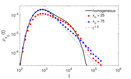
Figure 3: FPT probability density $\rho_{x_{0}}(t)$ for symmetric HCTRW on a discrete interval with $N=100$ sites, the absorbing endpoint at $x^{*}=1$, and the reflecting endpoint at $x=100$. We set $x_{0}=50$, $\tau=1$, and $\tilde{\psi}_{xx^{\prime}}(s)=(1+s\tau)^{-1}$ for all $x$, except for a trapping site at $x_{h}$ for which $\tilde{\psi}_{x_{h}x^{\prime}}(s)=(1+(s\tau)^{\alpha})^{-1}$, with $\alpha=0.5$. Two cases $x_{h}=25$ and $x_{h}=75$ are compared to the homogeneous case without trapping site (solid line). Dashed line shows a power law decay $t^{-1-\alpha}$.

Second, we demonstrate the effect of adding a single trapping site with reversible binding kinetics. For this purpose, we consider the homogeneous interval with $\tilde{\psi}_{xx^{\prime}}(s)=(1+s\tau)^{-1}$, except for one point $x_{h}$, at which $\tilde{\psi}_{x_{h}x^{\prime}}(s)=(1+(s\tau)^{\alpha})^{-1}$, with a scaling exponent $\alpha=0.5$. This corresponds to the Mittag-Leffler distribution of exchange times. Since the mean waiting time at the trapping site is infinite, a random walker can remain trapped much longer at this particular site, as compared to other sites. Figure 3 shows the probability density $\rho_{x_{0}}(t)$ with $x_{0}=50$ for three cases: no trapping site (the reference case), trapping site at $x_{h}=25$ and trapping site at $x_{h}=75$. The two latter cases are qualitatively different because the walker is always trapped at $x_{h}=25$ on the way to the sink at $x^{*}=1$, whereas the trapping site at $x_{h}=75$ may be not be visited when started at $x_{0}=50$. In the latter case, the density $\rho_{x_{0}}(t)$ coincides with that for the homogeneous case at short times because the short trajectories to the sink do not pass through the trapping site at $x_{h}=75$. In turn, significant deviations appear at long times. Indeed, eventual traps with the infinite mean trapping time drastically changes the propagator so that the density $\rho_{x_{0}}(t)$ exhibits a slow, power law long-time asymptotic decay: $\rho_{x_{0}}(t)\propto t^{-1-\alpha}$, in analogy to Eq. (27). In particular, the mean FPT to the sink is infinite, regardless the position of the trap.

Figure 4: FPT probability density $\rho_{x_{0}}(t)$ for symmetric HCTRW on a discrete interval with $N=100$ sites, the absorbing endpoint at $x^{*}=1$, and the reflecting endpoint at $x=100$. We set $x_{0}=100$, $\tau=1$, and $\tilde{\psi}_{xx^{\prime}}(s)=(1+s\tau_{x})^{-1}$, with four choices: $\tau_{x}=\tau$ (homogeneous case), $\tau_{x}=\tau(1+0.5\sin(4\pi x/N))$, $\tau_{x}=ax$ (linear increase), $\tau_{x}=a(N+1-x)$ (linear decrease), with $a=2\tau/(N(N+1))$.

Third, we look at the effect of spatial variations of the mean travel time $\tau_{x}$ by setting $\tilde{\psi}_{xx^{\prime}}(s)=(1+s\tau_{x})^{-1}$. Such a HCTRW can be viewed as a microscopic model of heterogeneous diffusion processes with space-dependent diffusion coefficient Cherstvy13 ; Pineda2014 which can also mimic crowding effects Ghosh16 . We consider four choices for $\tau_{x}$: a constant, $\tau_{x}=\tau$ (the reference case); a periodic variation, $\tau_{x}=\tau(1+c\sin(q\pi x/N))$; a linear growth from the sink, $\tau_{x}=ax$; and a linear decrease towards the sink, $\tau_{x}=a(N+1-x)$. For a proper comparison of these cases, we choose the functions $\tau_{x}$ to have the same mean travel time over the interval. We use the arithmetic mean: $\frac{1}{N}\sum\nolimits_{x=1}^{N}\tau_{x}=\tau$, as justified below. In particular, we set $a=\frac{2\tau}{N(N+1)}$ and take $q$ to be an integer (one also imposes $|c|<1$ to ensure the positivity of $\tau_{x}$). Figure 4 shows the probability density $\rho_{x_{0}}(t)$ at $x_{0}=100$ for these cases. As expected, periodic variations of the mean travel time have no effect on the first passage time, in comparison to the homogeneous case. In fact, these variations are averaged out by passing through all the sites. This observation justifies our choice of using the arithmetic mean: the first passage time can be viewed as a weighted sum of travel times between visited sites. We also checked that the probability density $\rho_{x_{0}}(t)$ does not depend on the amplitude $c$ and the frequency $q$ for a broad range of these parameters (not shown). In turn, if the starting point $x_{0}$ is not set at a site with $\tau_{x_{0}}=\tau$ (here, at $x_{0}=100$), then differences between the homogeneous and periodic cases can emerge. For instance, if $q=1$, $c>0$, and $x_{0}=25$, then a walker would on average take longer travel times, as $\tau_{x}>\tau$ for $x$ between $1$ and $50$. This difference is particularly important at short times.

Now we turn to the linear dependence of $\tau_{x}$ on $x$. The spatial heterogeneity of travel times strongly affects the probability density $\rho_{x_{0}}(t)$: the distribution of FPT is much wider in the case when the mean travel time $\tau_{x}$ increases from the sink site, $\tau_{x}=ax$, as compared to the case of decreasing $\tau_{x}=a(N+1-x)$. Indeed, the probability density $\rho_{x_{0}}(t)$ at long times is determined by long trajectories, which stayed away from the sink. Since the random walker samples preferentially the sites far from the sink, the FPT to the sink is longer in the case of linearly increasing $\tau_{x}$ and shorter in the case of linearly decreasing $\tau_{x}$. The argument is inverted at short times when the density $\rho_{x_{0}}(t)$ is determined by short trajectories when the walker moves preferentially towards the sink.

IV Conclusions

We presented a new model of heterogeneous continuous time random walks, which generalizes CTRW by allowing a heterogeneous distribution of travel times between sites. This model merges two important and rapidly developing research directions: continuous-time random walks as a generic model of anomalous transport, and discrete-time random walks on graphs and networks. We derived the analytical formula (10) for the HCTRW propagator in the Laplace domain and discussed its inversion to time domain. In particular, the perturbative analysis of the matrix $I-\tilde{Q}(s)$ yields the long-time asymptotic behavior. More generally, the complex diffusive dynamics in multiscale structures with spatio-temporal heterogeneities was related to the spectral properties of the generalized transition matrix $\tilde{Q}(s)$. In this light, a rigorous extension of this study to infinite graphs (or, equivalently, the limit of increasing graphs) presents an important perspective. In this situation, the steady-state distribution may not exist (as for a simple random walk on an infinite lattice), whereas the spectrum of the generalized stochastic matrix may be continuous. The derivation of a macroscopic description of HCTRW on very large (or infinite) graphs Asz1993 , like fractional diffusion equation for CTRW, remains an open problem. This analysis can shed a light onto space-dependent diffusion equations and provide their microscopic models.

In order to reveal the effects of spatio-temporal heterogeneities onto the diffusive dynamics, we kept the geometric structure as simple as possible. The next step consists in coupling these heterogeneities to the structural complexity of graphs and networks Albert02 ; Noh04 ; Colizza07 ; Sood07 ; Haynes09 ; Nicolaides10 ; Barthelemy11 ; Holme12 ; Perra12 ; Hwang12 ; Skarpalezos13 ; Goutsias13 ; Kozak14 ; Bovaventura14 ; Agliari16 . For instance, one can study HCTRW on some fractal trees and networks, for which the spectral properties are relatively well known Grabow12 ; Julati2013 ; Sole-Ribalta13 . Even a simple random walk on fractal structures such as tree graphs, in combination with the particular distributions of waiting times, often leads to anomalous diffusion Tamm2015 ; Spanner16 . Since coarse-graining methods have been extensively developed over the last decade Vocka00 ; Picard07 ; Klimenko12 ; Varloteaux13 , the HCTRW framework has a promising application for studying transport properties in porous materials. Other potential applications include transportation systems (with the intricate interrelation between the traffic and the complex topology of the roads graph or airflight connections), electric networks, as well as internet and social networks Barrat04 ; Noulas15 .

Appendix A Basic properties and technical relations

A.1 Reduction to Montroll-Weiss formula

We show that HCTRW framework leads to the Montroll-Weiss formula for CTRW on a lattice Montroll1973 . The spatial and temporal components of the waiting time distribution of CTRW are separated:

$$Q_{x^{\prime}x}(t)=Q_{x^{\prime}x}\psi(t),$$ (32)

where $\psi(t)$ is the waiting time probability density. Then Eq. (10) becomes

$$\tilde{P}_{x_{0}x}(s)=\frac{1-\tilde{\psi}(s)}{s}[(I-Q\tilde{\psi}(s))^{-1}]_{x_{0}x}.$$ (33)

For one-dimensional lattice ${{\mathbb{Z}}}$, the discrete Fourier transform yields

$${\mathcal{F}}_{k}\{\tilde{P}_{x_{0}x}(s)\} =\sum\limits_{x=\infty}^{\infty}\tilde{P}_{x_{0}x}(s)e^{ikx}$$ (34)

$$=e^{ikx_{0}}\frac{1-\tilde{\psi}(s)}{s}\frac{1}{1-\tilde{\psi}(s)(1-\lambda_{k}^{0})}.$$ (35)

This is the Montroll-Weiss formula for CTRW in Laplace-Fourier domain, where $1-\lambda_{k}^{0}=qe^{-ik}+(1-q)e^{ik}$ is the characteristic function of the jump distribution on the lattice, with probability $q$ (resp., $1-q$) to jump to the left (resp., to the right). The calculation extends to ${{\mathbb{Z}}}^{d}$ with $d$-dimensional discrete Fourier transform.

A.2 Spectrum of the generalized transition matrix

Since $\tilde{\psi}_{xx^{\prime}}(s)$ is the Laplace transform of a probability density of a positive random variable, one has $\tilde{\psi}_{xx^{\prime}}(s)\geq 0$, $\tilde{\psi}_{xx^{\prime}}(0)=1$, and

$$\tilde{\psi}_{xx^{\prime}}(s+\delta)-\tilde{\psi}_{xx^{\prime}}(s)=\int_{0}^{\infty}\psi_{xx^{\prime}}(t)e^{-ts}(e^{-\delta t}-1)dt<0$$

for any $\delta>0$ (we excluded the trivial distribution with $\psi_{xx^{\prime}}(t)=\delta(t)$, for which the integral is equal to $0$). As a consequence, $\tilde{\psi}_{xx^{\prime}}(s)$ is a monotonously decreasing function on $(0,\infty)$, and thus

$$0\leq\tilde{\psi}_{xx^{\prime}}(s)<1\qquad(s>0).$$ (36)

The matrix $\tilde{Q}(s)$ is a real (nonsymmetric) matrix with nonnegative elements. We note that the matrix $\tilde{Q}(s)$ is not necessarily irreducible that allows us to consider, e.g., sink sites. According to the Perron-Frobenius theorem for nonnegative matrices, there exists a nonnegative eigenvalue $\lambda_{0}$ such that the corresponding eigenvector $v_{0}$ has nonnegative components, and the other eigenvalues $\lambda_{k}$ are bounded in the absolute value: $|\lambda_{k}|\leq\lambda_{0}$. Since the sum of the elements of the matrix $\tilde{Q}_{xx^{\prime}}(s)$ in each column does not exceed $1$, one gets $\lambda_{0}\leq 1$. In fact, denoting $v_{0}(x)$ the maximal component of the vector $v_{0}$, $v_{0}(x)=\max\limits_{x^{\prime}}\{v_{0}(x^{\prime})\}>0$, one has

$$\lambda_{0}v_{0}(x)=\sum\limits_{x^{\prime}}\tilde{Q}_{xx^{\prime}}v_{0}(x^{\prime})\leq\max\limits_{x^{\prime}}\{v_{0}(x^{\prime})\}\sum\limits_{x^{\prime}}\tilde{Q}_{xx^{\prime}}\leq v_{0}(x)$$

that implies $\lambda_{0}\leq 1$. Moreover, the inequality is strict for $s>0$ due to Eq. (36). As a consequence, the matrix $I-\tilde{Q}(s)$ is invertible for any $s>0$.

A.3 Normalization of the HCTRW propagator

We check the normalization of the HCTRW propagator. From Eq. (10) we get:

$$\sum_{x}\tilde{P}_{x_{0}x}(s)=$$ (37)

$$\frac{1}{s}\sum_{x}(1-\sum_{x^{\prime}}\tilde{Q}(s)_{xx^{\prime}})[(I-\tilde{Q}(s))^{-1}]_{x_{0}x}=$$

$$\frac{1}{s}\sum_{x,x^{\prime}}\bigg{[}(I-\tilde{Q}(s))^{-1}\bigg{]}_{x_{0}x}\bigg{[}(I-\tilde{Q}(s))\bigg{]}_{xx^{\prime}}=\frac{1}{s}.$$

So that $\sum_{x}P_{x_{0}x}(t)=1$ for any $t$ and $x_{0}$.

The normalization of the approximate expression Eq. (15) is also fulfilled:

$$\sum_{x}(\sum_{x^{\prime}}T_{xx^{\prime}})[(I-Q+sT)^{-1}]_{x_{0}x}=$$ (38)

$$\sum_{x,x^{\prime}}[(I-Q+sT)^{-1}]_{x_{0}x}T_{xx^{\prime}}=$$

$$\sum_{x^{\prime}}[(I-Q+sT)^{-1}T]_{x_{0}x^{\prime}}=$$

$$\frac{1}{s}\sum_{x^{\prime}}[(I-Q+sT)^{-1}(sT+I-Q-(I-Q))]_{x_{0}x^{\prime}}=$$

$$\frac{1}{s}\bigg{(}1-\sum_{x,x^{\prime}}[(I-Q+sT)^{-1}]_{x_{0}x}[I-Q]_{xx^{\prime}}\bigg{)}=\frac{1}{s},$$

where the last implication is valid because $\sum_{x^{\prime}}[(I-Q)]_{xx^{\prime}}=0$, independently of $x$ and $s$.

A.4 Stationary distribution of a simple random walk on a graph

We recall the basic result about the stationary distribution of a simple random walk on a graph $G=(V,E)$ with $E$ for the set of edges. In this model, the transition probability from $x^{\prime}$ to $x$ is $Q_{x^{\prime}x}=1/\deg_{x^{\prime}}$, where $\deg_{x^{\prime}}$ denotes the number of edges incident with the node $x^{\prime}$. The stationary distribution is $\pi_{x}=\deg_{x}/(2|E|)$, where $|E|$ is the number of edges. In fact, we have

$$\sum_{x^{\prime}}\pi_{x^{\prime}}Q_{x^{\prime}x}=\sum_{x^{\prime}\in{\mathcal{A}}(x)}\frac{\deg_{x^{\prime}}}{2|E|}\,\frac{1}{\deg_{x^{\prime}}}=\frac{\deg_{x}}{2|E|}=\pi_{x},$$ (39)

where the sum runs over all sites $x^{\prime}$ adjacent to $x$ (for other sites $Q_{x^{\prime}x}$ is zero). We get thus $\pi Q=\pi$.

A.5 No dependence on $\psi_{x^{*}x^{*}}(t)$

As intuitively expected, the propagator in the presence of a sink at $x^{*}$ does depend on the choice of the corresponding travel time probability density $\psi_{x^{*}x^{*}}(t)$. For simplicity of notations, let $x^{*}=1$ so that the governing matrix has the form

$$H=\left(\begin{array}[]{c c c c}\phi&0&0&\ldots\\ &&&\\ &&\hat{H}&\\ &&&\\ \end{array}\right),$$ (40)

where $\phi=1-\tilde{\psi}_{x^{*}x^{*}}(s)$ and $\hat{H}$ is the remaining matrix of size $(N-1)\times N$. The elements of the inverse of $H$ can be formally written in terms of minors as

$$\tilde{P}_{x_{0}x}(s)=\frac{1-\sum\nolimits_{x^{\prime}}\tilde{Q}_{xx^{\prime}}(s)}{s}\,\frac{(-1)^{x_{0}+x}{\textrm{det}}({{\mathcal{M}}}_{xx_{0}}(H))}{{\textrm{det}}(H)},$$ (41)

where ${{\mathcal{M}}}_{xx_{0}}(H)$ is the matrix obtained from $H$ by removing the row $x$ and the column $x_{0}$. We consider separately two cases: $x\neq x^{*}$ and $x=x^{*}$:

(i) In the former case, the first factor in Eq. (41) does not contain $\tilde{\psi}_{x^{*}x^{*}}(s)$. Using the Laplace’s formula and the structure of the matrix $H$, one gets ${\textrm{det}}(H)=\phi~{}{\textrm{det}}({{\mathcal{M}}}_{x^{*}x^{*}}(H))$. Similarly, ${\textrm{det}}({{\mathcal{M}}}_{xx_{0}}(H))=\phi~{}{\textrm{det}}({{\mathcal{M}}}_{x^{*}x^{*}}({{\mathcal{M}}}_{xx_{0}}(H)))$ so that the factor $\phi$ containing $\tilde{\psi}_{x^{*}x^{*}}(s)$ is canceled, whereas the remaining minors do not contain $\phi$.

(ii) In the case $x=x^{*}$, Eq. (41) becomes

$$\tilde{P}_{x_{0}x^{*}}(s)=\frac{\phi}{s}\,\frac{(-1)^{x_{0}+x}{\textrm{det}}({{\mathcal{M}}}_{x^{*}x_{0}}(H))}{\phi~{}{\textrm{det}}({{\mathcal{M}}}_{x^{*}x^{*}}(H))},$$ (42)

where we used that $\tilde{Q}_{x^{*}x^{\prime}}=\delta_{x^{*}x^{\prime}}\tilde{\psi}_{x^{*}x^{*}}(s)$. Once again, the factor $\phi$ is canceled whereas the minors ${{\mathcal{M}}}_{x^{*}x_{0}}(H)$ and ${{\mathcal{M}}}_{x^{*}x^{*}}(H)$ do not contain $\phi$. We conclude that the propagator $\tilde{P}_{x_{0}x}(s)$ does not depend on $\tilde{\psi}_{x^{*}x^{*}}(s)$.

Appendix B Explicit solutions for circular graphs

In general, a numerical Laplace inversion is needed to get the HCTRW propagator in time domain. Here we provide an example when the inversion can be performed explicitly.

Figure 5: $m$-circular graph with $N=10$ nodes is shown for $m=2$ (left) and $m=4$ (right). Arrows indicate possible jumps to neighboring nodes.

Let us consider the asymmetric random walk on a $m$-circular graph (also known as a regular small-world graph) with $N$ nodes, where the degree $m$ of each node is even (Fig. 5). Such graphs have a circular transition matrix $Q$ with $m$ non-zero elements in each row Mieghem . Let us set transition probabilities for each node to be $2q/m$ (jumps to the “right”) and $2(1-q)/m$ (jumps to the “left”). We also choose $\tilde{\psi}_{xx^{\prime}}(s)$ to be equal to $\tilde{\psi}_{+}(s)$ for jumps to the right and to $\tilde{\psi}_{-}(s)$ for jumps to the left. The components of an eigenvector of the circular matrix $I-\tilde{Q}(s)$ are given by:

$$v_{k}(x) =e^{2\pi ikx/N}/\sqrt{N},$$ (43)

where $k=0,1,\ldots,N-1$ and $x=1,\ldots,N$. Denoting $\gamma=e^{2\pi i/N}$, the eigenvalues $\lambda_{k}(s)$ of $I-\tilde{Q}(s)$ are:

$$\lambda_{k}(s) =1-q\tilde{\psi}_{-}(s)\gamma_{k}-(1-q)\tilde{\psi}_{+}(s)\gamma_{-k},$$ (44)

where

$$\gamma_{k}=\frac{2}{m}\,\frac{1-e^{2\pi ikm/(2N)}}{e^{-2\pi ik/N}-1}.$$ (45)

These spectral quantities fully determine the propagator in the Laplace domain according to Eq. (10).

In the particular case of exponential distributions $\tilde{\psi}_{\pm}(s)=(1+s\tau_{\pm})^{-1}$, one easily gets the explicit form of the propagator in time domain. For this purpose we represent $\lambda_{k}(s)$ as

$$\lambda_{k}(s)=\frac{\tau_{+}\tau_{-}s^{2}+B_{k}s+C_{k}}{(1+s\tau_{+})(1+s\tau_{-})},$$ (46)

where

$$B_{k} = (\tau_{+}+\tau_{-})-\tau_{+}q\gamma_{k}-\tau_{-}(1-q)\gamma_{-k},$$

$$C_{k} = 1-q\gamma_{k}-(1-q)\gamma_{-k}.$$

Since $C_{0}=0$, one has

$$\lambda_{0}(s)=\frac{\tau_{+}\tau_{-}s(s+{\omega})}{(1+s\tau_{+})(1+s\tau_{-})},$$ (47)

where ${\omega}=(1-q)/\tau_{-}+q/\tau_{+}$. As a consequence, the Laplace transform of the propagator is

$$\tilde{P}_{x_{0}x}(s) =\frac{1}{sN}+\frac{1}{N}\sum\limits_{k=1}^{N-1}\frac{e^{2\pi ik(x-x_{0})/N}}{{s}_{k}^{+}-{s}_{k}^{-}}$$ (48)

$$\times\biggl{(}\frac{{\omega}+{s}_{k}^{+}}{s-{s}_{k}^{+}}-\frac{{\omega}+{s}_{k}^{-}}{s-{s}_{k}^{-}}\biggr{)},$$

where

$$s_{k}^{\pm}=\frac{-B_{k}\pm\sqrt{B_{k}^{2}-4\tau_{+}\tau_{-}C_{k}}}{2\tau_{+}\tau_{-}}.$$

The Laplace inversion yields the propagator in time domain:

$$P_{x_{0}x}(t) =\frac{1}{N}+\frac{1}{N}\sum_{k=1}^{N-1}\frac{e^{2\pi k(x-x_{0})/N}}{s^{+}_{k}-s^{-}_{k}}$$ (49)

$$\times\biggl{(}(\omega+s^{+}_{k})e^{s^{+}_{k}t}-(\omega+s^{-}_{k})e^{s^{-}_{k}t}\biggr{)}.$$

In the case of Mittag-Leffler distribution of travel times, $\tilde{\psi}_{\pm}(s)=1/(1+s^{\alpha}\tau_{\pm}^{\alpha})$, one can simply replace $s$ by $s^{\alpha}$ and $\tau_{\pm}$ by $\tau_{\pm}^{\alpha}$ in the above expressions for $\lambda_{k}(s)$, $B_{k}$, $\omega$, and $s_{k}^{\pm}$. As a consequence, the propagator in time domain reads

$$P_{x_{0}x}(t)=\frac{1}{N}+\frac{1}{N}\sum_{k=1}^{N-1}\frac{e^{2\pi k(x-x_{0})/N}}{s^{+}_{k}-s^{-}_{k}}$$ (50)

$$\times\biggl{(}(\omega+s^{+}_{k})E_{\alpha}(s^{+}_{k}t^{\alpha})-(\omega+s^{-}_{k})E_{\alpha}(s^{-}_{k}t^{\alpha})\biggr{)},$$

where $E_{\alpha}(z)$ is the Mittag-Leffler function.

References

- (1) J.-P. Bouchaud and A. Georges, Phys. Rep. 195, 127-293 (1990).
- (2) M. Sahimi, Rev. Mod. Phys. 65, 1393 (1993).
- (3) M. O. Coppens, Cat. Today 53, 225 (1999).
- (4) A. Plassais, M.-P. Pomies, N. Lequeux, J.-P. Korb, D. Petit, F. Barberon, and B. Bresson, Phys. Rev. E 72, 041401 (2005).
- (5) Y.-Q. Song, S. Ryu, and P. N. Sen, Nature 406, 178 (2000).
- (6) J. W. Kirchner, X. Feng, and C. Neal, Fractal stream chemistry and its implications for contaminant transportin catchments Nature 403, 524 (2000).
- (7) B. Berkowitz, H. Scher, and S. E. Silliman, Water Resour. Res. 36, 149 (2000).
- (8) B. Berkowitz, J. Klafter, R. Metzler, and H. Scher, Water Resources Res. 38 10, 1191 (2002).
- (9) H. Scher, G. Margolin, R. Metzler, J. Klafter, and B. Berkowitz, Geophys. Res. Lett. 29, 1061 (2002).
- (10) L. K. Gallos, C. Song, S. Havlin, and H. A. Makse, Proc. Nat. Acad. Sci. USA 104, 7746 (2007).
- (11) M. Dentz, H. Scher, D. Holder, and B. Berkowitz, Phys. Rev. E 78, 041110 (2008).
- (12) A. Zoia, C. Latrille, and A. Cartalade, Phys. Rev. E 79, 041125 (2009).
- (13) H. Scher, K. Willbrand, and B. Berkowitz, Phys. Rev. E 81, 031102 (2010).
- (14) B. Berkowitz and H. Scher, Phys. Rev. E 81, 011128 (2010).
- (15) P. Bressloff and J. M. Newby, Rev. Mod. Phys. 85, 135 (2013).
- (16) R. Metzler, J.-H. Jeon, A. G. Cherstvy, and E. Barkai, Phys. Chem. Chem. Phys. 16, 24128 (2014).
- (17) A. S. Serov, C. Salafia, D. S. Grebenkov, and M. Filoche, J. Appl. Physiol. 120, 17-28 (2016).
- (18) M. Sahimi, Phys. Rev. E 85, 016316 (2012).
- (19) P. E. Levitz, Statistical Modeling of Pore Networks (pp. 35-80), in Handbook of Porous Solids, Eds. F. Schüth, W. S. W. Sing, J. Weitkamp, vol. 1 (Wiley-VCH, 2002).
- (20) P. Levitz, V. Tariel, M. Stampanoni, and E. Gallucci, Eur. Phys. J. Appl. Phys. 60, 24202 (2012).
- (21) E. Montroll and G. Weiss, J. Math. Phys. 6, 167 (1965).
- (22) E. W. Montroll, J. Math. Phys. 10, 753 (1969).
- (23) E. Montroll and H. Scher, J. Stat. Phys. 9, 101 (1973).
- (24) R. Metzler, J. Klafter, and I. M. Sokolov, Phys. Rev. E 58, 1621 (1998).
- (25) R. Metzler and J. Klafter, J. Phys. A 37, R161 (2004).
- (26) E. Barkai, Chem. Phys. 284, 13-27 (2008).
- (27) P. K. Kang, M. Dentz, T. Le Borgne, and R. Juanes, Phys. Rev. Lett. 107, 180602 (2011).
- (28) I. Fouxon and M. Holzner, Phys. Rev. E 94, 022132 (2016).
- (29) S. Amitai and R. Blumenfeld, J. Gran. Matt. 19, 1-9 (2017).
- (30) H. Scher and M. Lax, Phys. Rev. B 7, 4502 (1973).
- (31) V. Kenkre, E. Montroll, and M. Shlesinger, J. Stat. Phys. 9, 1, 45-50 (1973).
- (32) C. Van den Broeck and M. Bouten, J. Stat. Phys. 45, 1031 (1986).
- (33) F. Spitzer, Principles of random walks (Springer, New York, Berlin, Heidelberg, 2001).
- (34) J. Haus and K. Kehr, Phys. Rep. 150, 263-406 (1987).
- (35) G. H. Weiss, Aspects and Applications of the Random Walk (North-Holland, Amsterdam, 1994).
- (36) D. Mugnolo, Semigroup methods for evolution equations on networks (Springer-Verlag, Berlin, 2008).
- (37) I. Sokolov and J. Klafter, Phys. Rev. Lett. 97, 140602 (2006).
- (38) C. N. Angstmann, I. C. Donnelly, B. I. Henry, and T. A. M. Langlands, Phys. Rev. E 8̱8, 022811 (2013).
- (39) C. Carstensen, Numer. Math. 59, 349-360 (1991).
- (40) L. N. Trefethen and M. Embree, Spectra and pseudospectra: The Behavior of Nonnormal Matrices and Operators (Princeton, NJ Princeton University Press, 2005).
- (41) T. Kato, Perturbation theory for linear operators (Springer-Verlag, Berlin, Heidelberg, 1995).
- (42) M. M. Sternheim and F. Walker, Phys. Rev. C 6, 114 (1972).
- (43) M. Boguna, A. M. Berezhkovskii, and G. Weiss, Physica A 282, 475-485 (2000).
- (44) E. L. Wilmer, D. A. Levin, and Y. Peres, Markov Chains and Mixing Times (American Mathematical Society, 2009).
- (45) B. D. Hughes, Random walks and Random Environments (Clarendon, Oxford, 1995).
- (46) O. Zeitouni, Random Walks in Random Environment, Originally published in ḿissingEcole d’Été de Probabilités de Saint-Flour XXXI, 2001, Lecture Notes in Mathematics, 1837, 191-312 (Springer-Verlag Berlin Heidelberg, 2012).
- (47) M. Jaume and K. Lindenberg, Eur. Phys. J. B 90, 107 (2017).
- (48) P. V. Mieghem, Graph spectra (Cambridge University Press, 2011).
- (49) D. Griffiths, Introduction to Quantum Mechanics, (Prentice-Hall, Upper Saddle River, New Jersey, 1995).
- (50) J. Hunter, Lin. Alg. Appl. 82, 201-214 (1986).
- (51) L. Zou and Y. Jiang, Lin. Alg. Appl. 433, 1203-1211 (2010).
- (52) F. C. Collins and G. E. Kimball, J. Coll. Sci. 4, 425 (1949).
- (53) H. Sano and M. Tachiya, J. Chem. Phys. 71, 1276 (1979).
- (54) B. Sapoval, General Formulation of Laplacian Transfer Across Irregular Surfaces, Phys. Rev. Lett. 73, 3314 (1994).
- (55) D. S. Grebenkov, M. Filoche, and B. Sapoval, Eur. Phys. J. B 36, 221-231 (2003).
- (56) D. S. Grebenkov, Partially Reflected Brownian Motion: A Stochastic Approach to Transport Phenomena, “Focus on Probability Theory”, Ed. L. R. Velle, pp. 135-169 (Nova Science Publishers, 2006).
- (57) D. S. Grebenkov, Phys. Rev. E 76, 041139 (2007).
- (58) A. Singer, Z. Schuss, Osipov, and D. Holcman, SIAM J. Appl. Math. 68, 844 (2008).
- (59) D. S. Grebenkov, Phys. Rev. E 81, 021128 (2010).
- (60) F. Rojo, H. S. Wio, and C. E. Budde, Phys. Rev. E 86, 031105 (2012).
- (61) E. Abad, S. B. Yuste, and K. Lindenberg, Phys. Rev. E 81, 031115 (2010).
- (62) E. Abad, S. B. Yuste, and K. Lindenberg, Phys. Rev. E 86, 061120 (2012).
- (63) E. Abad, S. B. Yuste, and K. Lindenberg, Phys. Rev. E 88, 062110 (2013).
- (64) S. B. Yuste, E. Abad, and K. Lindenberg, Phys. Rev. Lett. 110, 220603 (2013).
- (65) E. Abad and J. J. Kozak, Phys. Rev. E 91, 022106 (2015).
- (66) B. Meerson, J. Stat. Mech. P05004 (2015).
- (67) B. Meerson and S. Redner, Phys. Rev. Lett. 114, 198101 (2015).
- (68) D. S. Grebenkov and J.-F. Rupprecht, J. Chem. Phys. 146, 084106 (2017).
- (69) S. Redner, A Guide to First-Passage Processes (Cambridge University Press, 2002).
- (70) Y. Lin and Z. Zhang, Phys. Rev. E 87, 062140 (2013).
- (71) A. Talbot, J. Inst. Maths. Applics. 23, 97-120 (1979).
- (72) A. G. Cherstvy, A. V. Chechkin, and R. Metzler, New J. Phys. 15, 083039 (2013).
- (73) I. Pineda, G. Chacon-Acosta, and L. Dagdug, Eur. Phys. J. Special topics 223, 3045-3062 (2014).
- (74) S. Ghosh, A. G. Cherstvy, D. S. Grebenkov, and R. Metzler, New J. Phys. 18, 013027 (2016).
- (75) L. Lovasz, Large Networks and Graph Limits Colloquium Publications. Vol. 60, (AMS, Providence, 2012).
- (76) R. Albert and A.-L. Barabási, Rev. Mod. Phys. 74, 47 (2002).
- (77) J. D. Noh and H. Rieger, Phys. Rev. Lett. 92, 118701 (2004).
- (78) V. Colizza, R. Pastor-Satorras, and A. Vespignani, Nature Phys. 3, 276 (2007).
- (79) V. Sood and P. Grassberger, Phys. Rev. Lett. 99, 098701 (2007).
- (80) C. P. Haynes and A. P. Roberts, Phys. Rev. E 79, 031111 (2009).
- (81) C. Nicolaides, L. Cueto-Felgueroso, and R. Juanes, Phys. Rev. E 82, 055101(R) (2010).
- (82) M. Barthelemy, Phys. Rep. 499, 1-101 (2011).
- (83) P. Holme and J. Saramäki, Phys. Rep. 519, 97-125 (2012).
- (84) N. Perra, A. Baronchelli, D. Mocanu, B. Goncalves, R. Pastor-Satorras, and A. Vespignani, Phys. Rev. Lett. 109, 238701 (2012).
- (85) S. Hwang, D.-S. Lee, and B. Kahng, Phys. Rev. Lett. 109, 088701 (2012).
- (86) L. Skarpalezos, A. Kittas, P. Argyrakis, R. Cohen, and S. Havlin, Phys. Rev. E 88, 012817 (2013).
- (87) J. Goutsias and G. Jenkinson, Phys. Rep. 5̱29, 199-263 (2013).
- (88) J. J. Kozak, R. A. Garza-Lopez, and E. Abad, Phys. Rev. E 89, 032147 (2014).
- (89) M. Bonaventura, V. Nicosia, and V. Latora, Phys. Rev. E 89, 012803 (2014).
- (90) E. Agliari, D. Cassi, L. Cattivelli, and F. Sartori, Phys. Rev. E 93, 052111 (2016).
- (91) C. Grabow, S. Grosskinsky, and M. Timme, Phys. Rev. Lett. 108, 218701 (2012).
- (92) A. Julaiti, W. Bin, and Z. Zhang, J. Chem. Phys. 138, 204116 (2013).
- (93) A. Solé-Ribalta, M. De Domenico, N. E. Kouvaris, A. Díaz-Guilera, S. Gómez, and A. Arenas, Phys. Rev. E 88, 032807 (2013).
- (94) M. V. Tamm, L. I. Nazarov, A. A. Gavrilov, and A. V. Chertovich, Phys. Rev. Lett. 114, 178102 (2015).
- (95) M. Spanner, F. Hoefling, S. C. Kapfer, K. R. Mecke, G. E.Schroeder-Turk, and T. Franosch, Phys. Rev. Lett. 116, 060601 (2016).
- (96) R. Vocka and M. A. Dubois, Phys. Rev. E 62, 5216 (2000).
- (97) G. Picard and K. Frey, Phys. Rev. E 75, 066311 (2007).
- (98) D. A. Klimenko, K. Hooman, and A. Y. Klimenko, Phys. Rev. E 86, 011112 (2012).
- (99) C. Varloteaux, M. Tan Vu, S. Békri, and P. M. Adler, Phys. Rev. E 87, 023010 (2013).
- (100) A. Barrat, M. Barthélemy, R. Pastor-Satorras, and A.Vespignani, Proc. Natl. Acad. Sci. U.S.A. 101, 3747 (2004).
- (101) A. Noulas, V. Salnikov, R. Lambiotte, and C. Mascolo, Eur. Phys. J. Data Science 4, 23 (2015).