Local sensitivity of spatiotemporal structures

Abstract

We present an index for the local sensitivity of spatiotemporal structures in coupled oscillatory systems based on the asymptotic scaling of local-in-space, finite-time Lyapunov Exponents. For a system of nonlocally-coupled Rössler oscillators, we show that deviations of this index reflect the sensitivity to noise and the onset of spatial chaos for the patterns where coherence and incoherence regions coexist.

Introduction

The investigation of synchronization and more complex spatiotemporal structures in coupled oscillatory and spatially extended systems is a predominant subject of nonlinear science [1, 2, 3, 4, 5, 6]. In recent years, after the discovery of structures with coexisting coherent and incoherent parts, so called chimera states, systems with nonlocal coupling are of particular interest [7, 8, 9, 10, 11, 12, 13, 14, 15, 16, 17, 18, 19, 20, 21, 22, 23, 24]. The temporal dynamics of individual elements in such a regime can be regular (stationary, periodic, quasi-periodic), chaotic, and even stochastic, see for example [22]. However, despite of the homogeneous coupling topology, not all elements necessarily display behavior of the same type. Typically, clusters are formed, which are characterized by coherent (almost synchronous) behavior of their constituent elements in time. Elements not belonging to such clusters exhibit irregular, incoherent behavior.

The chaotic nature of these incoherent ensembles is characterized by sensitive dependence on initial conditions and is quantitatively captured by the corresponding local rates of contraction and expansion along a trajectory, the so called Lyapunov exponents (LEs) [25, 26, 27, 28]. The maximal LE provides important information about the dynamics of the system as a whole: chaotic motion, when the maximal LE is positive and asymptotic convergence to steady state, when it is negative. Modern computer software facilitates the calculation of the full Lyapunov spectrum for ensembles consisting of a large number of oscillators [29, 30]. For instance, the work [31] studied the full Lyapunov spectrum of a chimera regime, as well as its dependence on an increasing number of ensemble elements. However, it is yet unclear how the maximal LE or full Lyapunov spectrum reflect the dynamical properties of an individual oscillator in a coupled system. Therefore, special characteristics for the local analysis in spatially-distributed systems have been considered in the literature. For instance, local Lyapunov Exponents [32] have been introduced to measure the exponential growth of perturbations localized in space. However in general, the computation of such local indicators for all spatially localized perturbations in large ensembles is numerically challenging.

In this article, we propose the following approach: The finite-time growth rate of the Lyapunov vector projected onto the subspace corresponding to a specific oscillator, which we call the index of local sensitivity (ILS). The ILS, in order words, measures the sensitivity of individual oscillators to external perturbations in a coupled system. It is computationally cheap in comparison, as it can be computed for all coupled elements in parallel. This article is organized as follows: Firstly, we introduce the needed mathematical concepts in more detail. Secondly, we show how the ILS performs for a system of nonlocally coupled Rössler oscillators in comparison with the conventional maximal Lyapunov Exponent. We study the relation between the spatial distribution of ILSs and the response of different oscillator ensembles to short-time noise. In particular, we show that elements with larger ILS-values are more sensitive to such perturbations, as it is expected. In addition, we reveal that the onset locus of spatial chaos can be characterized by the ILS: The incoherent part of the chimera state has larger ILS than the conventional maximum Lyapunov Exponent.

1 Index of local sensitivity: Definition and basic properties

For a given solution $\mathbf{x}$ of the system

$$\dot{\mathbf{x}}(t)=f(\mathbf{x}(t)),\quad\mathbf{x}(t)\in\mathbb{R}^{n},$$

the temporal evolution of a small perturbation vector $\boldsymbol{\xi}(t)$ from $\mathbf{x}(t)$ is characterized by the corresponding Lyapunov exponent (LE) $\lambda$ [28]. The LE is defined as

$$\lambda:=\limsup\limits_{T\to\infty}\Lambda(t_{0},T),$$ (1)

where

$$\Lambda(t_{0},T):=\dfrac{1}{T}\ln\dfrac{\|\boldsymbol{\xi}(t_{0}+T)\|}{\|\boldsymbol{\xi}(t_{0})\|},$$ (2)

is the finite-time growth rate of a small perturbation $\boldsymbol{\xi}(t_{0})$ from $\mathbf{x}(t)$ at time $t_{0}$ governed by the linearized system

$$\dot{\boldsymbol{\xi}}(t)=Df(\mathbf{x}(t))\boldsymbol{\xi},\quad\boldsymbol{\xi}(t)\in\mathbb{R}^{n}.$$

The spectrum of Lyapunov exponents consists of (up to) $n$ numbers $\lambda_{1}\geq\lambda_{2}\geq,\dots,\geq\lambda_{n}$ corresponding to different initial perturbations $\boldsymbol{\xi}(t_{0})$, see e.g. [33] for details. In particular, $\lambda_{1}=\max_{i=1,\dots n}\lambda_{i}$ is called the maximal Lyapunov exponent, $\lambda_{\max}$ for short. For a generic initial perturbation $\boldsymbol{\xi}(t_{0})$, the definition (1) leads to the maximal LE. To remind the reader, when $\lambda_{\max}$ is positive, the system displays sensitive dependence on initial conditions and is chaotic. If alternatively, the maximal LE is negative, any small perturbation asymptotically converges to $\mathbf{x}$. However, this convergence can be very slow and preceded by long chaotic transients, as the finite-time growth rates $\Lambda(t_{0},T)$ can still be positive for large intervals of time [34]. In this way, the finite-time growth rates provide additional information about the dynamics of $\mathbf{x}$.

When we consider an ensemble of oscillators consisting of $N$ elements, each of them described by $k$ independent variables, the full system has a phase space of dimension equal to $n=Nk$. Here, the $Nk$-dimensional perturbation vector $\boldsymbol{\xi}(t)$ can be represented as $\boldsymbol{\xi}(t)=\left(\boldsymbol{\xi}_{1}(t),\dots,\boldsymbol{\xi}_{N}(t)\right)$, where $\boldsymbol{\xi}_{i}(t)\in\mathbb{R}^{k},\,i\in\left\{1,2,\dots,N\right\}$ is the projection to the subspace corresponding to the $i$-th oscillator. We propose a new characteristic measuring the response of oscillator $i$ to a homogeneous perturbation of the form $\boldsymbol{\xi}(t_{0})=\left(\boldsymbol{\xi}_{1}(t_{0}),\dots,\boldsymbol{\xi}_{1}(t_{0})\right)$: The finite-time growth rate of the Lyapunov vector projected onto the subspace corresponding to this oscillator, which we call the index of local sensitivity (ILS) and which we define as

$$\Lambda_{i}(t_{0},T):=\dfrac{1}{T}\ln\dfrac{\|\boldsymbol{\xi}_{i}(t_{0}+T)\|}{\|\boldsymbol{\xi}_{i}(t_{0})\|}=\dfrac{1}{T}\ln\sqrt{N}\dfrac{\|\boldsymbol{\xi}_{i}(t_{0}+T)\|}{\|\boldsymbol{\xi}(t_{0})\|}.$$ (3)

The ILS is related to the finite-time LE, as

$$e^{2\Lambda(t_{0},T)T}=\dfrac{1}{N}\sum_{i=1}^{N}e^{2\Lambda_{i}(t_{0},T)T}$$

and in some sense, it can be represented as a mean of the individual contributions of the ILSs to the maximal LE

$$\lambda_{\max}=\limsup_{T\to\infty}\dfrac{1}{2T}\ln\dfrac{1}{N}\sum_{i=1}^{N}e^{2\Lambda_{i}(t_{0},T)T}.$$ (4)

By replacing $\Lambda(t_{0},T)$ by $\lambda_{\max}$ here, we assumed that the homogeneous perturbation is ’’generic’’ in the sense that it is not contained in the subspace corresponding to smaller Lyapunov exponents $\lambda_{2},\dots,\lambda_{n}$. In the specific case, when all oscillators are synchronized, all indices of local sensitivity are identical ($\Lambda_{0}(t_{0},T)=\Lambda_{1}(t_{0},T)=\dots=\Lambda_{N}(t_{0},T)$), and it holds

$$\limsup_{T\to\infty}\Lambda_{i}(t_{0},T)=\lambda_{\max}.$$ (5)

Even though the ILS can asymptotically converge to the maximal Lyapunov exponent for less coherent ensembles, the direction (from above or from below) and the speed provide valuable information about the finite-time ’’sensitivity’’ of a particular oscillator. In the following sections, we numerically investigate the dependence of the ILS on the index $i$, as well as on the reference time $T$. For brevity, from now on, we omit the dependence on $t_{0}$ and when numerical results are presented, the associated spatial profile $\mathbf{x}_{i}(t_{0})$ will be clearly stated, where it is appropriate.

2 Nonlocally coupled Rössler oscillators

To showcase the approach, we use a system of $N$ nonlocally coupled chaotic Rössler oscillators, which are known to demonstrate various spatiotemporal structures, including chimera states [35]. The system under consideration is described by the following set of $3N$ ordinary differential equations:

$$\begin{array}[]{l}\dot{x}_{i}(t)=-y_{i}(t)-z_{i}(t)+\dfrac{\sigma}{2P}\sum\limits_{k=i-P}^{i+P}\left(x_{k}(t)-x_{i}(t)\right),\\ \dot{y}_{i}(t)=x_{i}(t)+ay_{i}(t)+\dfrac{\sigma}{2P}\sum\limits_{k=i-P}^{i+P}\left(y_{k}(t)-y_{i}(t)\right),\\ \dot{z}_{i}(t)=b+z_{i}(t)(x_{i}(t)-c)+\dfrac{\sigma}{2P}\sum\limits_{k=i-P}^{i+P}\left(z_{k}(t)-z_{i}(t)\right),\\[12.0pt] x_{i+N}(t)=x_{i}(t),\leavevmode\nobreak\ \leavevmode\nobreak\ y_{i+N}(t)=y_{i}(t),\\[6.0pt] z_{i+N}(t)=z_{i}(t),\leavevmode\nobreak\ \leavevmode\nobreak\ i=1,...N,\end{array}$$ (6)

such that the underlying coupling topology of the system is periodic, i.e. it is a nonlocal ring, where index $i$ determines the position of an oscillator, which is coupled to its $P$-nearest neighbors from each side with coupling strength $\sigma$. The parameters $a$, $b$, and $c$ determine the dynamics of an individual oscillator. For numerical purposes, we confine ourselves to $a=0.2$, $b=0.2$, and $c=4.5$, so that in the uncoupled case the dynamics of each element is chaotic. We consider an ensemble consisting of $N=300$ oscillators, each one coupled to its $P=100$ nearest neighbors. In the following, we numerically compute the ILS for different values of the coupling strength and relate the results to the temporal dynamics of the system, in order to familiarize the reader with this approach.

2.1 Complete incoherence versus complete chaotic synchronization

At first we contrast two limiting cases: Complete spatial incoherence and the regime of complete synchronization. For small positive values of the coupling strength $\sigma\approx 0$, one observes complete spatial incoherence [36, 37]. Here for randomly chosen initial conditions, each individual element is chaotic, and at a fixed moment in time the spatial distribution does not exhibit any apparent coherent ensemble. The corresponding ILSs $\Lambda_{i}(T)$ are shown in Fig. (1)(a) alongside an example of spatial distribution of the oscillators $x_{i}$, see Fig. (1)(a, inset).

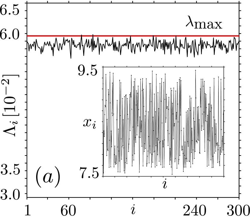
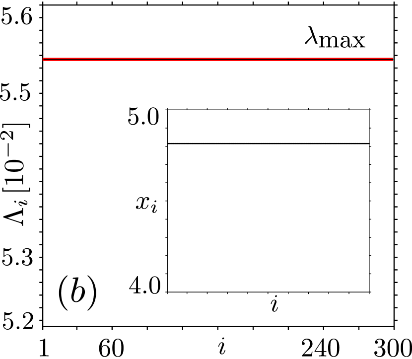
Figure 1: (Color online) Spatial distribution of ILS $\Lambda_{i}(T),\,T=10^{4}$ in the regime of complete spatial incoherence (a) $\sigma\geq 0$ small, and complete coherence (b) $\sigma\gg 1$. Panels show $\Lambda_{i}(T)$ versus $i$ in comparison with the maximal LE $\lambda_{\text{max}}$ (red). The inset in (a), respectively (b), shows the spatial distribution of $x_{i}$ at a fixed instant of time.

Naturally in this case, the ILS are close to the maximal LE with some local variation among the oscillators, as finite-time LE do not depend continuously on the initial condition. Note that in this case all $\Lambda_{i}$ attain smaller values than the maximal LE, as it corresponds to the direction along which the expansion is maximal. Increasing the coupling strength $\sigma$ to large values, complete chaotic synchronization can be observed in the system [38, 39, 40, 41]. In this regime, after some transient, all elements still oscillate chaotically, but synchronously so, with $\mathbf{x}_{i}(t)=\mathbf{x}_{j}(t)$, for all $i,j$. As the dynamics of the oscillators is identical, all $\Lambda_{i}(T)$ coincide and as $T\to\infty$, they converge to the maximal Lyapunov exponent up to the precision given by the resolution of Fig. 1(b). For a corresponding example spatial distribution of the oscillators $x_{i}$ see Fig. (1)(b, inset). We have made a simple observation here: incoherent (coherent) ensembles of oscillators posses incoherent (coherent) ILS. Throughout this paper, we will exploit this fact and investigate how the value and scaling of ILSs reflect dynamical properties of the system state and what additional information can be obtained from the ILS.

2.2 Partial chaotic synchronization

For intermediate values of the coupling, one can observe partial coherence between the individual chaotic oscillators [35]. Solutions in this regime are characterized by piecewise smooth instantaneous spatial profiles, see Fig. 2(a), where almost all adjacent elements of the ensemble oscillate approximately synchronously, but two distant elements can have (possibly very) different instantaneous states. For example, the solution shown in Fig. 2(a) is almost coherent in space: small (large) values of oscillator $\mathbf{x}_{i}$ correspond to small (large) values of $\mathbf{x}_{j}$ for all $j$. However, it exhibits two points of discontinuity in its spatial profile at the oscillators $i=85$, and $i=240$ respectively, such that it can be thought of as two clusters of oscillators $i=1,\dots,85,240,\dots,300$ and $i=85,\dots,240$ each one coherent in space.

The distribution of ILSs $\Lambda_{i}(T)$ along this solution is shown in Fig. 2(b). We observe that it varies continuously in space and has a pronounced maximum about oscillator $i=160$, where $\Lambda_{i}(T)>\lambda_{\text{max}}$, which corresponds to local rates of expansion higher than the maximum Lyapunov exponent. This observation contrasts with our intuition that the maximal sensitivity of the ensemble must be observed in the regions around the profile distortions. Surprisingly, the minima of the ILS distribution are observed around the points, where the spatial profile is discontinuous.

Our numerical simulations show that the range of $\Lambda_{i}(T)$, that is $R_{\text{ILS}}(T):=\max_{i}\Lambda_{i}(T)-\min_{i}\Lambda_{i}(T)$ decreases with time 2(c) and asymptotically, all sensitivity indices $\Lambda_{i}(T)$ have approximately the same value $\lambda_{\max}$ Fig. 2(b). The qualitative explanation for this effect is as follows: for $T\rightarrow\infty$ the vector of perturbation of the whole system line up with the direction corresponding to the maximal Lyapunov exponent [28, 42]. This perturbation is changing along the phase trajectory, however, the lengths of all the projections of a perturbation vector in partial oscillators are changed proportionally. In the limit, any projection either increases or decreases exponentially with the same rate, which is determined by the value of the maximal Lyapunov exponent $\lambda_{\max}$.

We emphasize that the variation of ILS for different oscillators is an effect of the finite calculation time $T$. In order to use this characteristic, one should choose it in an optimal way: small enough to avoid the asymptotic limit (in our case study of the Rössler system $T<10^{4}$), and large enough to exceed the characteristic timescale of the system. Interestingly, we observe that, although the local variation in $\Lambda_{i}(T)$ decreases, the local maxima and minima of the spatial ILS profile remain over time, see Fig. 2(d). The ILS distribution rescaled by $R_{\text{ILS}}$ forms a characteristic shape providing qualitative and quantitative information about the sensitivity of different oscillators in the ensemble.

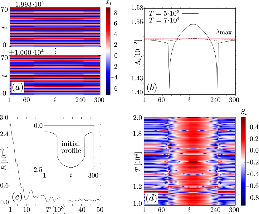
Figure 2: (Color online) Spatial distribution of $\Lambda_{i}(T)$ in the regime of partial synchronization of chaotic dynamics for intermediate coupling strength $\sigma=0.05$. Panel (a) shows an example trajectory of the system for $t\in[10^{4},2\cdot 10^{4}]$ in a spatiotemporal plot. Panel (b) shows the corresponding spatial distribution of the ILS $\Lambda_{i}(T)$ for $T=5\cdot 10^{3}$ (solid line), $T=7\cdot 10^{4}$ (dotted line) and the maximal LE $\lambda_{\text{max}}$ of the full system along this solution. One observes that $\Lambda_{i}(T)$ converges to $\lambda_{\text{max}}$ and the local minima along the spatial distribution correspond to the boundaries between the two clusters. Panel (c) shows the spatial range of ILSs $R_{\text{ILS}}(T)=\max_{i}\Lambda_{i}(T)-\min_{i}\Lambda_{i}(T)$ versus the reference time T for a fixed initial profile (inset). Panel (d) shows the temporal evolution of the rescaled ILS $S_{i}(T)=(\Lambda_{i}(T)-\Lambda(T))/R_{\text{ILS}}(T)$.

3 Index of local sensitivity: Results

3.1 Local sensitivity to noise

In this section, we study the impact of a noisy perturbation on a partially coherent solution as shown in Fig. (2)(a). We relate our findings to the ILS distribution (Fig. (3)(a)) and reveal how the deviations in $\Lambda_{i}(T)$ influence the response of an individual oscillators. In particular, we show that the oscillators $i$ with small ILS correspond to stable (with respect to noise) regions of the profile, see Fig. (3)(b, region I). On the other hand, oscillators with ILS locally higher than the maximal LE, $\Lambda_{i}(T)>\lambda_{\text{max}}$, respond to external perturbation more strongly, see Fig. (3)(b, region II).

To do so, we consider the following stochastic system

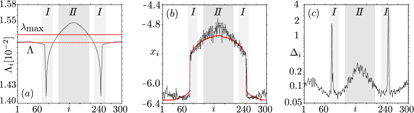
Figure 3: (Color online) Influence of uniform noise with low intensity $D=10^{-5}$ on the spatial structure in the regime of partial synchronisation $\sigma=0.05$, see also Fig. 2. Panel (a) shows ILS distribution $\Lambda_{i}(T)$ versus $i$ for $T=5\cdot 10^{3}$ (black, solid), the finite-time LE $\Lambda_{i}(T)$ for $T=5\cdot 10^{3}$ (red, dashed) and the maximal LE $\lambda_{\text{max}}$ (red, solid). Spatial Regions I (Oscillators $i$ with $\Lambda_{i}(T)<\Lambda(T)$) and II (Oscillators $i$ with $\Lambda_{i}(T)>\lambda_{\text{max}}$) are highlighted in every panel. Panel (b) shows the influence of noise (black) on a spatial profile (red). Panel (c) shows the degree of incoherence $\Delta_{i}$ averaged over $t\in[5\cdot 10^{3},7\cdot 10^{4}]$.

$$\begin{array}[]{l}\dot{x}_{i}=-y_{i}-z_{i}+\dfrac{\sigma}{2P}\sum\limits_{k=i-P}^{i+P}\left(x_{k}-x_{i}\right)+\sqrt{2D(i,t)}n(t),\\ \dot{y}_{i}=x_{i}+ay_{i}+\dfrac{\sigma}{2P}\sum\limits_{k=i-P}^{i+P}\left(y_{k}-y_{i}\right)+\sqrt{2D(i,t)}n(t),\\ \dot{z}_{i}=b+z_{i}(x_{i}-c)+\dfrac{\sigma}{2P}\sum\limits_{k=i-P}^{i+P}\left(z_{k}-z_{i}\right)+\sqrt{2D(i,t)}n(t),\\[12.0pt] \end{array}$$ (7)

with periodic boundary conditions, as in (6). Here, $n(t)$ is a normalized source of Gaussian white noise with intensity $D(i,t)$.

In order to measure the effect of noise applied to the system, we use the quantity

$$\Delta_{i}=\langle(2x_{i}(t)-x_{i+1}(t)-x_{i-1}(t))^{2}\rangle$$ (8)

as the degree of the local incoherence of the spatial profile at point $i$, see [23, 43] for more details. Here, the averaging $\langle\cdot\rangle$ is performed with respect to time. This characteristic displays the averaged ’’curvature’’, as the expression $\left(2x_{i}(t)-x_{i+1}(t)-x_{i-1}(t)\right)^{2}$ is a measure of the local deviation from the linear state. $\Delta_{i}$ admits small values for coherent states and larger values for incoherent as it is shown in [23].

At first, we consider a constant noise intensity $D(i,t)\equiv D$, uniform for all time $t$ and oscillators $i$. Figure 3(b) shows an example profile in space for a fixed instant of time with and without noise. The corresponding distribution of $\Delta_{i}$ in space is shown in Fig. 3(c), where the time averaging is performed for $5\cdot 10^{3}$ time units. The distinct peaks in Fig. 3(c, region I) correspond to the profile distortion. At the same time, the maximum of $\Delta_{i}$ in region II, coincides with the maximum in the ILS distribution in the plots in Figs. 3(a). Thus, the elements with the largest values of $\Lambda_{i}(T)$ are most sensitive to the noise influence, in contrast to the elements, which are characterized by smaller values of ILS.

Additionally, when studying the influence of localized short-time noise,

$$\begin{array}[]{l}D(i,t)=\begin{cases}D,\leavevmode\nobreak\ \leavevmode\nobreak\ i\in[i_{1};i_{2}]\,\,\mbox{and}\,\,t\in[0,T_{n}],\\ 0,\leavevmode\nobreak\ \leavevmode\nobreak\ \,\,\mbox{otherwise,}\end{cases}\end{array}$$ (9)

where $\left[i_{1},i_{2}\right]$ is the spatial and $[0,T_{n}]$ the temporal interval of the noise action, we can relate the value of the ILS, to the characteristic decay time of this perturbation. We consider the system (7) without noise to be in the regime of partial coherence, as studied above (Fig. 2), with noise parameters chosen as $D=0.05$ and $T_{n}=0.1$. Figure (4) exhibits the spatiotemporal plot of two local perturbations applied in regime I (low ILS, Fig. (4)(a)), and regime II (high ILS, Fig. (4)(b)) respectively. One can observe that the perturbation in the high-sensitive region II persists significantly longer then in the low-sensitive region I. Thus, the ILS can serve as a sensitivity measure to noisy perturbations. The non-coherent response, which is induced by the localized short-time high-intensity influence of noise, persists significantly longer in the case when the perturbation is applied to a high-sensitive region (with higher ILS) than in case of the influence to the region with low values of ILS. The obtained results indicate the non-homogeneity of the response of system (6) in the regime of partial coherence.

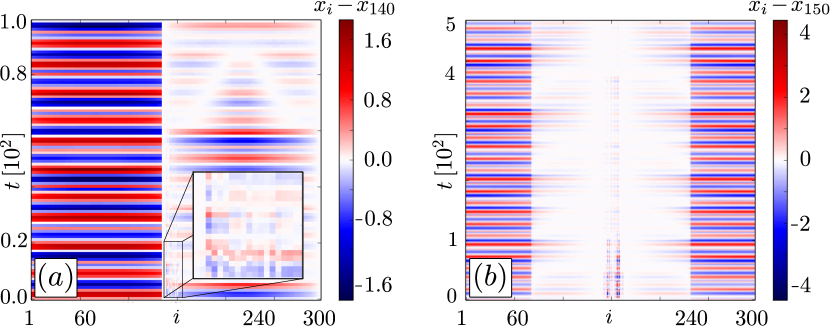
Figure 4: (Color online) Influence of spatially localized short-time noise with intensity $D=0.05$ in the regime of partial synchronization of chaotic dynamics for intermediate coupling strength $\sigma=0.05$. Panels (a) and (b) show the spatiotemporal evolution of a perturbation in regions I (a) and II (b) (see Fig. 3 for the definition of regions I and II) in a corresponding reference frame: $x_{i}-x_{140}$ in (a) and $x_{i}-x_{150}$ in (b). In panel (a), oscillator numbers are shifted such that the perturbation appears centered.

3.2 Local sensitivity of chimera states

In the regime of partial chaotic synchronization, so called ’’chimera’’ states have been observed. There are 2 main flavors in which a spatially coherent profile can become locally incoherent [21]: (1) An oscillator that is close to the boundary of two coherent clusters, say cluster 1 and 2, can be irregularly ‘‘shifted’’ in space with respect to the instantaneous phase of adjacent oscillators belonging to cluster 1, but the oscillator itself has values comparable to an oscillator in cluster 2: the so-called ‘‘phase’’ chimera, which needs to be distinguished from a ‘‘chimera of phase oscillators’’. (2) In an ‘‘amplitude’’ chimera, the oscillators locally possess an irregular spatial distribution with respect to the surrounding cluster. So naturally, phase chimeras occur in the region of low ILS (compare region I in Fig. 3(a)) and amplitude chimeras in the region of high ILS (compare region II in Fig. 3(a)). In this section, we numerically investigate the distributions of ILS for these regimes.

Firstly we study the phase chimera shown in Fig. 5(a). Here, elements of the incoherent cluster oscillate almost periodically in time. Their instantaneous amplitudes are almost identical (changes smoothly with $i$), and the adjacent elements oscillate either in-phase or anti-phase. Moreover, these shifts are irregularly distributed in space. It has been argued that this chimera type is stable in time and resistant to external influence [44], which is also reflected by the ILS. Figure 5(b) shows the distribution of ILSs $\Lambda_{i}(i)$ rescaled by their range $R_{\text{ILS}}(T)$ corresponding to the phase chimera in (a). The ILS distribution in the coherence cluster changes smoothly leading to the similar sensitivity of adjacent elements. On the contrary, the ILS of the incoherence cluster varies irregularly and most importantly has lower ILS than the oscillators in the coherent clusters.

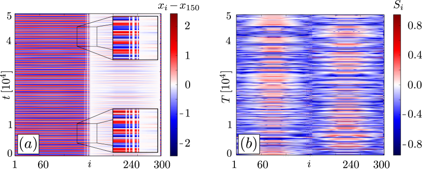
Figure 5: (Color online) Spatial distribution of $\Lambda_{i}(T)$ in the regime of partial coherence (‘‘phase’’ chimera) of chaotic dynamics for coupling strength $\sigma=0.044$. Panel (a) shows the temporal evolution of the oscillators $x_{i}$ with respect to oscillator $150$ that is part of the incoherent ensemble. Panel (b) shows the temporal evolution of the rescaled ILS $S_{i}(T)=(\Lambda_{i}(T)-\Lambda(T))/R_{\text{ILS}}(T)$. (In panels (a) and (b) oscillator numbers have been shifted, such that the chimera state appears centered)

An example of amplitude chimera is presented in Fig. 6(a). Amplitude chimeras in ensembles of chaotic oscillators are presumably metastable states, unlike for the phase chimeras. They exist for a finite (but possibly very long) time [44] and are regarded as sensitive to perturbations in the form of noise.

Fig. 6(b) represents the spatial distribution of $\Lambda_{i}(T)$ rescaled by range $R_{\text{ILS}}(T)$ in the regime of the amplitude chimera. The ILS distribution is continuous in the coherence cluster, while the values of $\Lambda_{i}(T)$ can significantly vary for the elements of the incoherence cluster. The ILS has a maximum in the region of an incoherence cluster, unlike the phase chimera. Thus, the region of an amplitude chimera is the least stable part of the spatial structure.

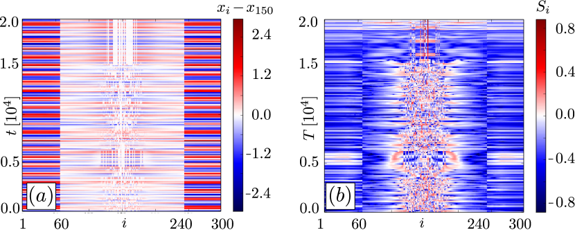
Figure 6: (Color online) Spatial distribution of $\Lambda_{i}(T)$ in the regime of partial coherence (‘‘amplitude’’ chimera) of chaotic dynamics for coupling strength $\sigma=0.04$. Panel (a) shows the temporal evolution of the oscillators $x_{i}$ with respect to oscillator $150$ that is part of the incoherent ensemble. Panel (d) shows the temporal evolution of the rescaled ILS $S_{i}(T)=(\Lambda_{i}(T)-\Lambda(T))/R_{\text{ILS}}(T)$. (In panels (a) and (b) oscillator numbers have been shifted, such that the chimera state appears centered)

Conclusion

We are convinced that the index of local sensitivity enriches the numerical toolbox for the study of spatiotemporal structures and the fast growing field of network analysis. There are two major reasons for this:

(1) It has a clear interpretation in terms of the finite-time growth rate of perturbations to a specific oscillator. We have shown that this interpretation is indeed valid, as the value of ILS is related to the decay time of perturbations by short-time noise applied to a specific oscillator. In this way, we are able to identify elements, which are most sensitive to small perturbations (including noise). This information is important for the development and evaluation of methods to influence single oscillators and larger ensembles by an external control and to improve the structure of a general network in order to render it more robust to external perturbations. From a theoretical point of view, we showed that the ILS provides valueable information in the study of complex spatial structures, as it can predict the onset locus of spatial chaos in the case of chimera states in a system of coupled Rössler oscillators.

(2) It is computationally cheap, such that it can be applied to coupled systems with a large number of elements. As a finite-time measurement, it can be calculated for a varying range of timescales that, needless to say, need to be adjusted to the phenomenon under consideration. We plan to investigate the scaling behavior of the ILS as $T\to\infty$ in more detail, as for the solutions we considered, each ILS converges to the maximum Lyapunov Exponent of the full system (up to numerical intergration error). Here, many questions arise: Does the distribution of ILSs rescaled by $R_{ILS}$ converge to an asymptiotic shape? Does negativity of an ILS imply local contraction and the spatiotemporal structure becomes fixed in time? For a general system, this of course need not necessarily be the case and there are many such open questions that can be investigated in the future.

References

- [1] A. Pikovsky, M. Rosenblum, and J. Kurths. Synchronization. A Universal Concept in Nonlinear Sciences. Cambridge University Press, 2001.
- [2] Y. Kuramoto. Chemical Oscillations, Waves and Turbulence. Springer-Verlag, Berlin, 1984.
- [3] V.S. Afraimovich, V.I. Nekorkin, G.V. Osipov, and V.D. Shalfeev. Stability, structures and chaos in nonlinear synchronization networks. World Scientific, Singapore, 1995.
- [4] V.I. Nekorkin and M.G. Velarde. Synergetic phenomena in active lattices. Springer, Berlin, 2002.
- [5] G.V. Osipov, J. Kurths, and Ch. Zhou. Synchronization in oscillatory networks. Springer, Berlin, 2007.
- [6] H. Malchow, S.V. Petrovskii, and E. Venturino. Spatiotemporal patterns in ecology and epidemiology: theory, models, and simulation. Chapman and Hall /CRC Press, London, 2007.
- [7] Y. Kuramoto and D. Battogtokh. Coexistence of Coherence and Incoherence in Nonlocally Coupled Phase Oscillators. Nonlin. Phen. in Complex Sys., 5(4):380–385, 2002.
- [8] D. M. Abrams and S. H. Strogatz. Chimera states for coupled oscillators. Phys. Rev. Lett., 93(17):174102, 2004.
- [9] O. Omelchenko, Yu.L. Maistrenko, and P.A.Tass. Chimera states: the natural link between coherence and incoherence. Phys.Rev.Lett., 100:044105, 2008.
- [10] Daniel M. Abrams, Rennie Mirollo, Steven H. Strogatz, and Daniel A. Wiley. Solvable Model for Chimera States of Coupled Oscillators. Physical Review Letters, 101(8):084103, August 2008.
- [11] Carlo R. Laing. Chimeras in networks of planar oscillators. Phys. Rev. E, 81:066221, Jun 2010.
- [12] I. Omelchenko, Y. Maistrenko, P. Hövel, and E. Schöll. Loss of coherence in dynamical networks: spatial chaos and chimera states. Phys. Rev. Lett., 106:234102, 2011.
- [13] O. E. Omel’chenko, M. Wolfrum, S. Yanchuk, Y. L. Maistrenko, and O. Sudakov. Stationary patterns of coherence and incoherence in two-dimensional arrays of non-locally-coupled phase oscillators. Phys. Rev. E, 85:036210, Mar 2012.
- [14] Aaron M. Hagerstrom, Thomas E. Murphy, Rajarshi Roy, Philipp Hovel, Iryna Omelchenko, and Eckehard Scholl. Experimental observation of chimeras in coupled-map lattices. Nat Phys, 8(9):658–661, September 2012.
- [15] E Omelchenko and Matthias Wolfrum. Nonuniversal transitions to synchrony in the sakaguchi-kuramoto model. Physical review letters, 109(16):164101, 2012.
- [16] E. Martens, S. Thutupalli, A. Fourriere, and O. Hallatschek. Chimera states in mechanical oscillator networks. Proc. Natl. Acad. Sci., 110:10563, 2013.
- [17] Tomasz Kapitaniak, Patrycja Kuzma, Jerzy Wojewoda, Krzysztof Czolczynski, and Yuri Maistrenko. Imperfect chimera states for coupled pendula. Scientific Reports, 4:6379–, September 2014.
- [18] Lennart Schmidt, Konrad Schönleber, Katharina Krischer, and Vladimir Garcia-Morales. Coexistence of synchrony and incoherence in oscillatory media under nonlinear global coupling. Chaos: An Interdisciplinary Journal of Nonlinear Science, 24(1):013102, 2014.
- [19] M. J. Panaggio and D. M. Abrams. Chimera states: Coexistence of coherence and incoherence in networks of coupled oscillators. Nonlinearity, 28:R67, 2015.
- [20] E. Schöll. Synchronization patterns and chimera states in complex networks: Interplay of topology and dynamics. The European Physical Journal Special Topics, 225(6-7):891–919, September 2016.
- [21] S. Bogomolov, A. Slepnev, G. Strelkova, E. Schöll, and V. Anishchenko. Mechanisms of appearance of amplitude and phase chimera states in a ring of nonlocally coupled chaotic systems. Commun. Nonlinear Sci. Numer. Simul., 43:25, 2017.
- [22] N. Semenova, A. Zakharova, V. Anishchenko, and E. Schöll. Coherence-resonance chimeras in a network of excitable elements. Phys. Rev. Lett., 117:014102, 2016.
- [23] I.A. Shepelev, A.V. Bukh, G.I. Strelkova, T.E. Vadivasova, and V.S. Anishchenko. Chimera states in ensembles of bistable elements with regular and chaotic dynamics. Nonlinear Dyn., 2017. Published online before print 18 September.
- [24] Joseph D. Hart, Kanika Bansal, Thomas E. Murphy, and Rajarshi Roy. Experimental observation of chimera and cluster states in a minimal globally coupled network. Chaos: An Interdisciplinary Journal of Nonlinear Science, 26(9):094801, 2016.
- [25] Lamberto Cesari. Asymptotic behavior and stability problems in ordinary differential equations, volume 16. Springer Science & Business Media, 2012.
- [26] F. Christiansen and H. H. Rugh. Computing lyapunov spectra with continuous gram - schmidt orthonormalization. Nonlinearity, 10(5):1063–1072, 1997.
- [27] V.B. Ryabov. Using lyapunov exponents to predict the onset of chaos in nonlinear oscillators. Phys. Rev. E, 66:16214, 2002.
- [28] Arkady Pikovsky and Antonio Politi. Lyapunov Exponents: A Tool to Explore Complex Dynamics. Cambridge University Press, 2016.
- [29] O. Popovych, Y. Maistrenko, and P. Tass. Phase chaos in coupled oscillators. Phys. Rev. E, 71(6):065201, 2005.
- [30] S.K. Patra and A. Ghosh. Statistics of lyapunov exponent spectrum in randomly coupled kuramoto oscillators. Phys. Rev. E, 93:032208, 2016.
- [31] M. Wolfrum, O. E. Omel’chenko, S. Yanchuk, and Y. Maistrenko. Spectral properties of chimera states. Chaos, 21:013112, 2011.
- [32] A.S. Pikovsky. Local lyapunov exponents for spatiotemporal chaos. Chaos, 3(2):225–232, 1993.
- [33] Stephen Wiggins. Introduction to Applied Nonlinear Dynamical Systems and Chaos, volume 2 of Texts in Applied Mathematics. Springer-Verlag New York, Inc., 2003.
- [34] A. Politi and A. Torcini. Stable chaos. In M. Thiel, J. Kurths, M. Romano, G. Károlyi, and A. Moura, editors, Nonlinear Dynamics and Chaos: Advances and Perspectives, pages 103–129. Springer, Berlin, Heidelberg, 2010.
- [35] I. Omelchenko, B. Riemenschneider, P. Hövel, Y. Maistrenko, and E. Schöll. Transition from spatial coherence to incoherence in coupled chaotic systems. Physical Review E, 85(2):026212, 2012.
- [36] A. Politi, F. Ginelli, S. Yanchuk, and Yu. Maistrenko. From synchronization to Lyapunov exponents and back. Physica D, 224:90–101, 2006.
- [37] M. G. Rosenblum, A. S. Pikovsky, and J. Kurths. Phase synchronization of chaotic oscillators. Phys. Rev. Lett., 76:1804–1807, 1996.
- [38] Louis M. Pecora and Thomas L. Carroll. Master stability functions for synchronized coupled systems. Phys. Rev. Lett., 80(10):2109–2112, March 1998.
- [39] L.M. Pecora, T.L. Carroll, G.A. Johnson, D.J. Mar, and J.F. Heagy. Fundamentals of synchronization in chaotic systems, concepts, and applications. Chaos, 7:520–543, 1997.
- [40] S. Yanchuk, Yu. Maistrenko, and E. Mosekilde. Loss of synchronization in coupled Rössler systems. Physica D, 154:26–42, 2001.
- [41] S. Yanchuk, Yu. Maistrenko, and E. Mosekilde. Synchronization of time-continuous chaotic oscillators. Chaos, 13:388–400, 2003.
- [42] F. Ginelli, P. Poggi, A. Turchi, H. Chaté, R. Livi, and A. Politi. Characterizing Dynamics with Covariant Lyapunov Vectors. Physical Review Letters, 99(13):130601, September 2007.
- [43] I.A. Shepelev, T.E. Vadivasova, A.V. Bukh, G.I. Strelkova, and V.S. Anishchenko. New type of chimera structures in a ring of bistable fitzhugh–nagumo oscillators with nonlocal interaction. Physics Letters A, 381(16):1398–1404, 2017.
- [44] N.I. Semenova, G.I. Strelkova, V.S. Anishchenko, and A. Zakharova. Temporal intermittency and the lifetime of chimera states in ensembles of nonlocally coupled chaotic oscillators. Chaos, 27(6):061102, 2017.