Deep Sampling Networks

Abstract

Deep convolutional neural networks achieve excellent image up-sampling performance. However, CNN-based methods tend to restore high-resolution results highly depending on traditional interpolations (e.g. bicubic). In this paper, we present a deep sampling network (DSN) for down-sampling and up-sampling without any cheap interpolation. First, the down-sampling subnetwork is trained without supervision, thereby preserving more information and producing better visual effects in the low-resolution image. Second, the up-sampling subnetwork learns a sub-pixel residual with dense connections to accelerate convergence and improve performance. DSN’s down-sampling subnetwork can be used to generate photo-realistic low-resolution images and replace traditional down-sampling method in image processing. With the powerful down-sampling process, the co-training DSN set a new state-of-the-art performance for image super-resolution. Moreover, DSN is compatible with existing image codecs to improve image compression.

1 Introduction

The aim of the image sampling is to generate a low-resolution (LR) image from a high-resolution (HR) image or reconstruct the HR image in reverse. Single-image up-sampling is widely used in computer vision applications including HDTV [1], medical imaging [2], satellite imaging [3], and surveillance [4], where high-frequency details are required on demand. As the use of mobile social networks (e.g., Google+, WeChat, and Twitter) continues to grow, thumbnail down-sampling is another important way to optimize data storage and transmission over limited-capacity channels.

Image up-sampling, also known as super-resolution (SR), has been studied for decades. Early methods including bicubic interpolation [5], Lanczos resampling [6], gradient profiles [7], and patch redundancy [8] are based on statistical image priors or internal patch representations. More recently, learning-based methods have been proposed to model a mapping from LR to HR patches such as neighbor embedding [9], sparse coding [10], and random forests [11]. However, image up-sampling is highly ill-posed, since the HR to LR process contains non-invertible down-sampling.

Due to their powerful learning capability, deep convolutional neural networks (CNNs) have achieved state-of-the-art performance in many computer vision tasks, such as image classification [12], object detection [13], and image segmentation [14]. Recently, CNNs have been used to address this ill-posed inverse problem, demonstrating superiority over traditional learning paradigms. The first example of the approach, super-resolution convolutional neural network (SRCNN) [15] predicted the nonlinear LR to HR mapping in an end-to-end manner. To reduce computational complexity, fast SRCNN (FSRCNN) [16] and efficient sub-pixel convolutional neural network (ESPCN) [17] up-scaled the resolution only at the output layer. Kim et al. [18] developed a very deep super-resolution (VDSR) network with 20 convolutional layers by residual learning, and Mao et al. [19] proposed a 30-layer residual encoder-decoder (RED) network with symmetric skip connections to facilitate training. Deeply-recursive convolutional network (DRCN) [20] introduced a very deep recursive layer via a chain structure with 16 recursions, and deep recursive residual network (DRRN) [21] adopted recursive residual units to control the model parameters while increasing depth.

Despite achieving excellent performance, the CNN-based methods are highly dependent on interpolation-based down/up-sampling, as shown in Fig. 1. The limitations of these methods arise from two aspects:

Figure 1: The classical framework based on CNNs for image up-sampling [15, 18, 19, 20, 21]. The HR image is down-sampled to synthesize the training samples. Then, the deep model learns the mapping between the HR and the cheap SR up-scaled by the same factor via bicubic interpolation.

Down-sampling. For down-sampling, the model trained for a specific interpolation does not work well with the other interpolations, and different interpolations significantly alter restoration accuracy. Therefore, all the solutions mentioned above generally assume that the degradation is a bicubic interpolation (the default setting of $imresize()$ in Matlab) when shrinking an image. However, the bicubic function based on a weighting transformation resprents a cheap down-sampling process that discards useful high-frequency details for HR image restoration.
Up-sampling. With cheap up-sampling, the networks [18, 19, 20, 21] increase the resolution during preprocessing or at the first layer to learn the interpolation’s residual. However, the up-sampling do not add information to solve the ill-posed restoration problem. To replace cheap interpolation, ESPCN [17] and FSRCNN [16] adopt sub-pixel shuffling and a deconvolution layer to improve efficiency, respectively. However, without cheap up-sampling, they carry the input and restore the details as an auto-encoder, so converge slowly.

To address the above problems, we propose a deep sampling network (DSN) without any cheap interpolation that is trained for simultaneous down- and up-sampling.

• A learnable down-sampling subnetwork (Down-SNet) is trained without supervision, thereby preserving more information and transmitting a better visual effect to the LR image. For self-supervision, the super-pixel residual is adopted with a novel activation function, called quantized bilateral ReLU (Q-BReLU).

• An up-sampling subnetwork (Up-SNet) learns a sub-pixel residual with dense connections to accelerate convergence and improve performance. First, the dense pixel representation trained with deep supervision extracts the multi-scale features by multi-level dictionaries, and second, the sub-pixel residual restores the HR result without cheap up-sampling.

Compare to traditional down-sampling methods, the Down-SNet can preserve more useful information and generate photo-realistic LR images. Compared to existing CNN-based up-sampling methods, the co-training DSN achieves the best performance with lower computational complexity.

2 CNN-based Sampling in Related Works

We first design an experiment to investigate the sampling in CNN-based SR methods. In this section, we re-implement the baseline SRCNN [15] model with the Adam [22] optimizer. The learning rate decreases by a factor of 0.1 from $10^{-3}$ to $10^{-5}$ every 50 epochs.

(a) Down-sampling

(b) Up-sampling

Figure 2: Convergence and accuracy analyses on different down/up-sampling methods.

2.1 Learn Restoration for Specified Down-sample

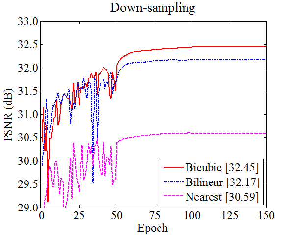
Almost all CNN-based SR methods [15, 16, 17, 19, 18, 20, 21, 23] are trained for a specified down-sampling. As shown in Table 1, down-sampling asymmetry in the training/testing phase results in poor restorations, even worse than the direct bicubic interpolation. This is because the CNNs learn the targeted mapping for the specified degradation. Moreover, different down-sampling (nearest-neighbor, bilinear, and bicubic) produce significantly different convergence rates and restoration accuracies shown in Fig. 2(a). The degradation with bicubic down-sampling contains more useful information, so the bicubic model converges faster and achieves better performance. However, the bicubic interpolation is still a cheap down-sampling process that discards useful details for HR image restoration. In this paper, we simultaneously train a deep sampling network for down-sampling and corresponding up-sampling.

Table 1: Comparison of different down-sampling degradations for scale factor $\times 3$ on Set5 [24] with PSNR (dB). The baseline PSNR of bicubic interpolation is 30.39.

	Nearest	Bilinear	Bicubic	Avg.
Nearest	30.59	29.76	30.56	30.30
Bilinear	25.38	32.17	31.19	29.58
Bicubic	27.59	31.92	32.45	30.70

2.2 Learn Mapping from Cheap Up-sample

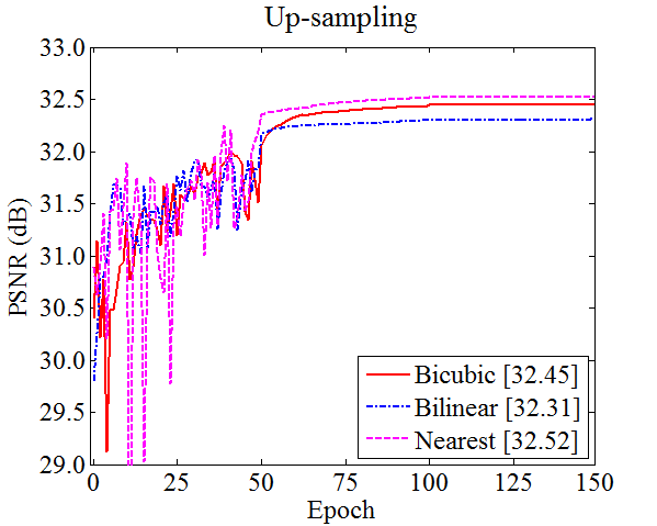
In the popular CNN-based SR methods (e.g. SRCNN [15], VDSR [18], DRCN [20], and DRRN [21]), cheap up-sampling is used during preprocessing to increase the resolution before or at the first network layer. As shown in Fig. 2(b), interpolations do not add information to improve restoration accuracy. Instead of improving accuracy, the complex (bicubic) preprocessing prematurely introduces smooth and inaccurate interpolation, resulting in a hard-to-train network. Conversely, the nearest-neighbor interpolation achieves the best performance because it selects the raw value of the nearest point and does not consider the values of neighboring points. To address this problem, ESPCN [17] and FSRCNN [16] carry the input and restore details without cheap up-sampling. However, deep information carry results in a decreasing convergence rate. Therefore, we propose sub-pixel residual learning to accelerate convergence and improve performance.

3 Deep Sampling Network

In this paper, we propose a deep sampling network (DSN) composed of a down-sampling subnetwork and an up-sampling subnetwork. The DSN architecture is presented in Fig. 3.

Figure 3: The deep sampling network. (1) The down-sampling subnetwork (Down-SNet) is trained in an unsupervised manner with super-pixel residual learning and the Q-BReLU function. (2) The up-sampling subnetwork (Up-SNet) learns the dense pixel representation by sub-pixel residual learning.

3.1 Unsupervised Down-sampling Subnetwork

A learnable down-sampling subnetwork (Down-SNet) is trained without supervision, which learns the super-pixel residual with a novel activation function, called quantized bilateral ReLU (Q-BReLU).

3.1.1 Super-pixel Residual Learning

Without a supervised signal, Down-SNet can proactively retain useful information and discard redundant information. However, the multi-layer network is an end-to-end relationship requiring very long-term memory. For this reason, the LR image generated from the learned features contains artifacts. We can simply solve this problem by super-pixel residual-learning.

In Down-SNet, the pixel of LR output $\textbf{L}_{x,y}$ of scale factor $1/s$ is largely similar to the super-pixel of the HR input H. Therefore, we define the super-pixel residual image for down-sampling $\textbf{R}_{x,y}^{d}={\textbf{L}_{x,y}}-\frac{1}{{\left|\Omega\right|}}\sum\nolimits_{\left\{{m,n}\right\}\in{\Omega_{s\cdot\left({x,y}\right)-\left\lfloor{s/2}\right\rfloor}}}{{\textbf{H}_{m,n}}}$, where $\left\lfloor{\cdot}\right\rfloor$ reduces the integer and $\Omega$ is a neighborhood with the size of $s\times s$. In $\textbf{R}^{d}$, most values are likely to be very low and even close to zero. Formally, the down-sampling is denoted $\mathcal{F}^{d}\left[\textbf{H}\right]\rightarrow\textbf{R}^{d}$, which includes an inference model (three convolutional layers of size $3\times 3$ and stride $1$) and a down-sampling layer (a convolutional layer of size $s\times s$ and stride of $s$). The original mapping is recast into

$${\textbf{L}_{x,y}}={\mathcal{F}^{d}}{\left[\textbf{H}\right]_{x,y}}+\frac{1}{{\left|\Omega\right|}}\sum\nolimits_{\left\{{m,n}\right\}\in{\Omega_{s\cdot\left({x,y}\right)-\left\lfloor{s/2}\right\rfloor}}}{{\textbf{H}_{m,n}}},$$ (1)

which can be implemented by feedforward neural networks with shortcut connections [25] and average pooling.

3.1.2 Quantized Bilateral ReLU (Q-BReLU)

Standard nonlinear activation functions such as the rectified linear unit (ReLU) offer local linearity to overcome the vanishing gradient problem. However, ReLU is designed for classification problems rather than image restoration. In particular, ReLU only inhibits values less than zero, which might lead to response overflow especially without supervision. Moveover, the general digital image is quantified to integers between 0 and 255.

To overcome this limitation, here we propose the quantized bilateral rectified linear unit (Q-BReLU) to keep bilateral restraint and response quantization, as shown in Fig. 4. Q-BReLU is a variation of BReLU [26], which is adopted for haze transmission restoration. BReLU is defined as ${f_{brelu}}=\max\left({\min\left({x,{t_{\max}}}\right),{t_{\min}}}\right)$, where $t_{\min,\max}$ is the marginal value. Denoting $\Delta t=t_{\max}-t_{\min}$ for terse expression, Q-BReLU is defined as

$$\begin{array}[]{l}{f_{qbrelu}}\left(x\right)=\\ \quad\;\;\;\frac{{\Delta t}}{{Q-1}}\left\lfloor{\frac{{Q-1}}{{\Delta t}}\left({{f_{brelu}}\left(x\right)-{t_{\min}}}\right)+0.5}\right\rfloor+{t_{\min}},\end{array}$$ (2)

where $Q$ is the number of quantities.

(a) Q-BReLU

(b) The gradient of Q-BReLU

Figure 4: The quantized bilateral rectified linear unit (Q-BReLU) with 2-bit quantities $Q=2^{2}$. (a) Q-BReLU is denoted in solid blue. (b) The approximate gradient of Q-BReLU is denoted in dashed red, and solid red denotes the spline fitting Q-BReLU.
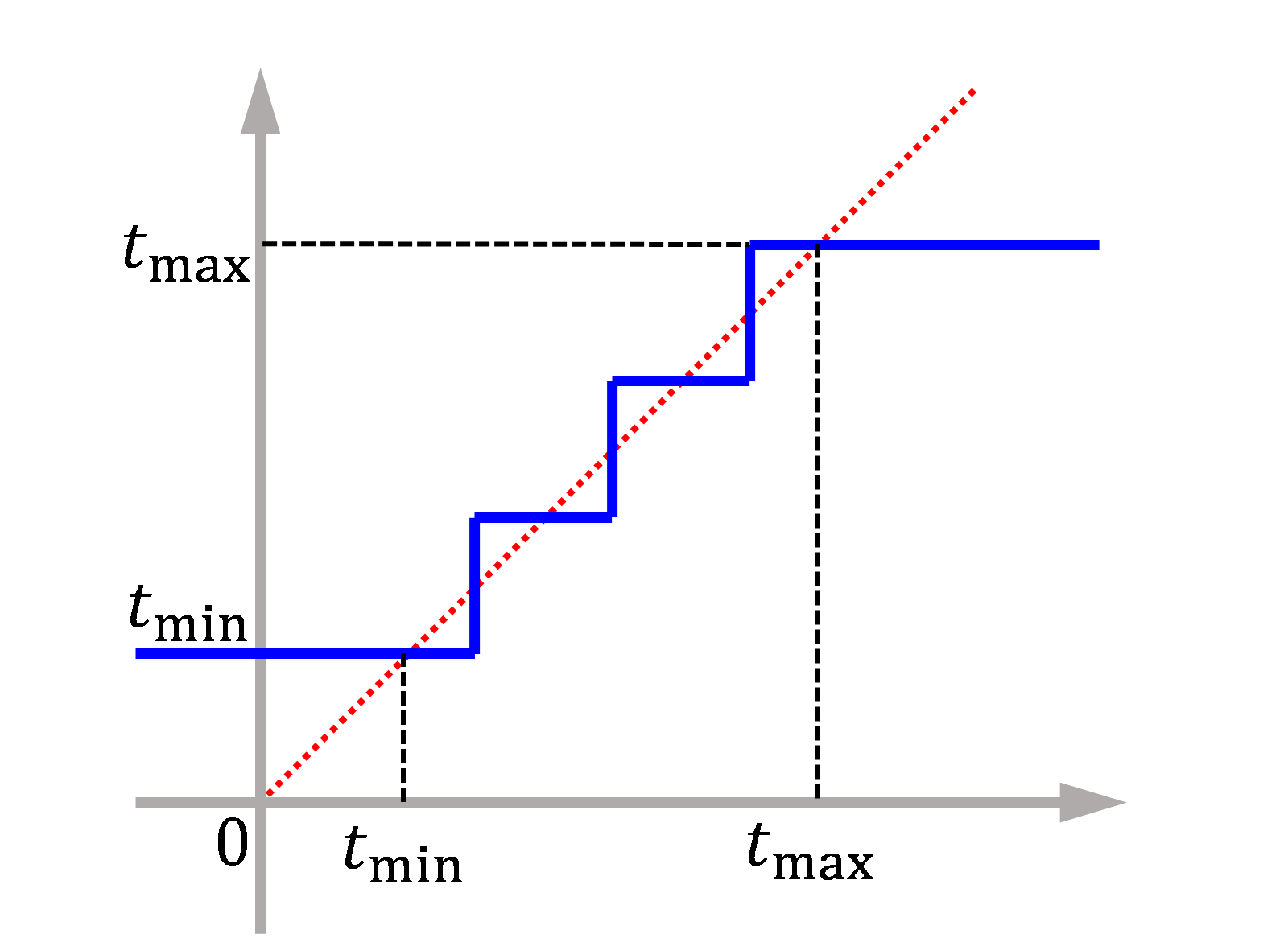
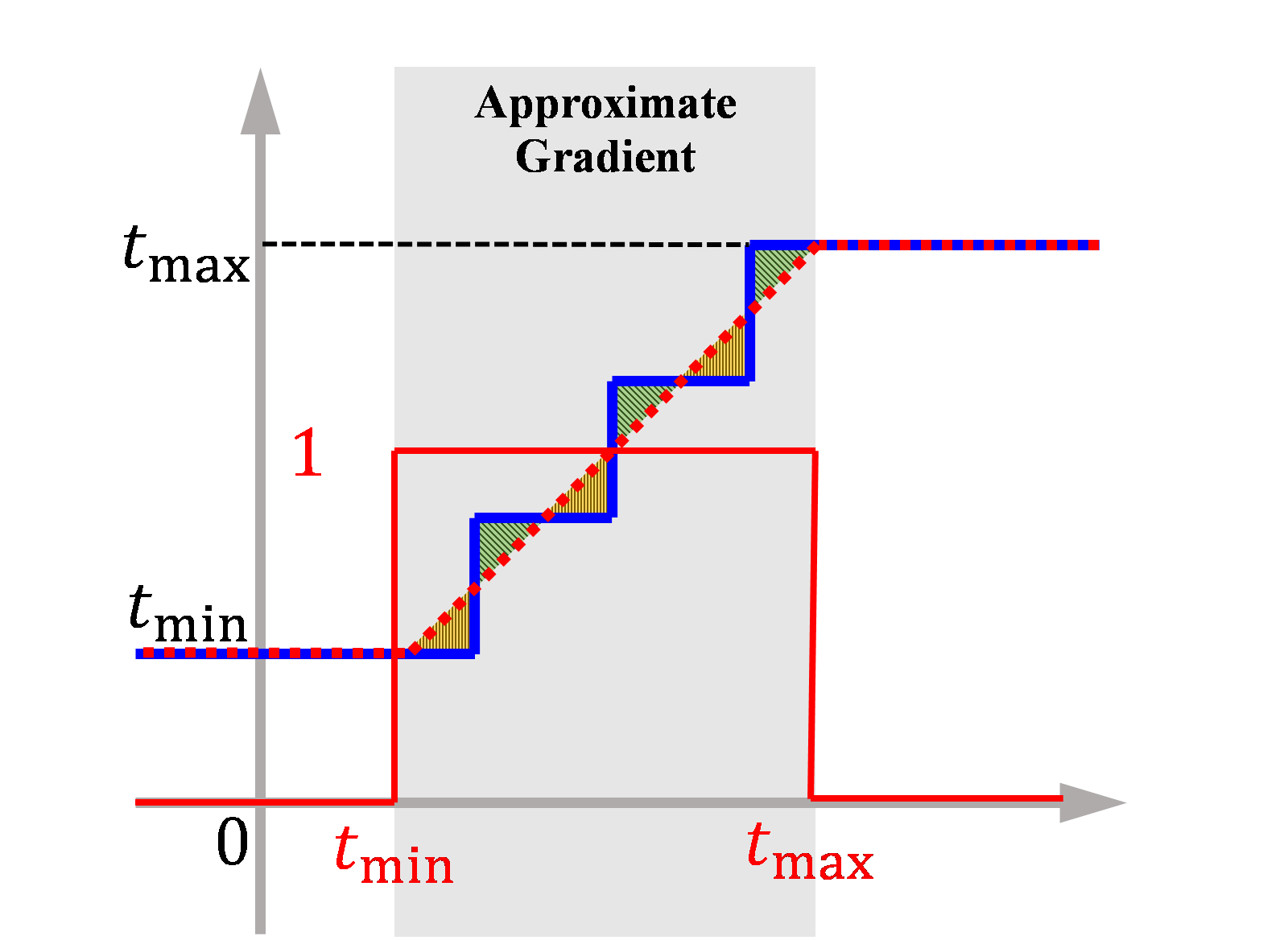
Center quantization: the high-precision value is rounded to the nearest quantization interval (between neighboring blue dashes); Zero mean deviation: the positive/negative (green/yellow area) deviation balance out the approximate bias.

However, the gradient of Q-BReLU alternates between 0 and $\infty$ according to (2). We exploit an approximate gradient with local continuity for backpropagation learning. To retain center quantization and zero mean deviation, BReLU is adopted as a spline function to fit Q-BReLU, as shown in Fig. 4(b). Therefore, the approximate gradient of Q-BReLU is defined as

$$\frac{{\partial{f_{qbrelu}}\left(x\right)}}{{\partial x}}=\left\{\begin{array}[]{l}1,\;{{t}_{\min}}<x<{{t}_{\max}}\\ 0,\;otherwise\end{array}\right..$$ (3)

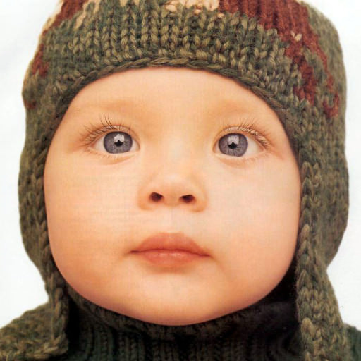
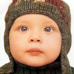
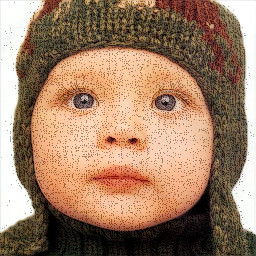
To verify the impact of Q-BReLU, we illustrate an example of $\times 2$ down-sampling in Fig. 5. The LR image generated without Q-BReLU contains irrational noise, while the result with Q-BReLU appears natural.

(a) HR

(b) Bicubic

(c) w/o Q-BReLU

(d) Q-BReLU

Figure 5: The images baby from Set5 [24] generated by DSN with or without Q-BReLU.

3.2 Residual Up-sampling Subnetwork

The up-sampling subnetwork (Up-SNet) is a dense architecture that learns the sub-pixel residual, achieving a high performance and efficiency without cheap interpolation.

3.2.1 Dense Pixel Representation

Up-SNet densely connects the pixel representation [27] for pixel-wise prediction. Each layer produces $k$ feature maps, so it follows that the $l$-th layer has $k\times l$ input feature maps. In the deep connection layers, a large number of feature maps increase the computational cost and model size. [28] demonstrated that a $1\times 1$ bottleneck convolution improves computational efficiency and keeps the model compact. The performance improvement of dense pixel representation come from three aspects:

1. Multi-scale feature. For up-scaling, different components may be relevant to different neighbourhood scales in the LR image. Up-SNet is a type of multi-scale, performance-improving architecture: the receptive field get larger when the network stacks more layers. Given a fixed kernel of size $3\times 3$, there are multi-scale streams corresponding to $\{3,5,7,9\}$ receptive fields, respectively.

2. Deeply-supervised learning. Image up-sampling is a low-level vision task, where the kernels in the shallow layers can be shared to recursively boost performance. However, recursions are hard to train due to exploding and/or vanishing gradients. Skip connections, similar to the deeply-supervised learning, overcome the vanishing gradient problem and enhance feature propagation.

3. Multi-level dictionaries. Sparse-coding is a representative example-based up-sampling method, where sparse coefficients are passed into a dictionary to restore HR patches. Up-SNet can be viewed as a type of sparse coding: convolutional kernels of size $3\times 3$ are equivalent to dictionaries, and the bottlenecks with nonlinear activation functions are equivalent to sparse coefficients. With dense connections, the neural unit learns multi-level dictionaries.

3.2.2 Sub-pixel Residual Learning

The HR image can be decomposed into low-frequency information (low-resolution image) and high-frequency information (residual image). In Up-SNet, the input image L and output image S share the same low-frequency information. Without any cheap interpolation, we adopt a sub-pixel residual learning to transmit the LR input to the HR result.

Depending on different sub-pixel location in HR space, the residual patterns containing $s^{2}$ channels are activated by a convolution of size $1\times 1$. Sub-pixel shuffle [17] is a periodic operator that rearranges the elements of an $H\times W\times s^{2}$ tensor to a tensor of shape $s\cdot H\times s\cdot W$. In the mathematica formula, the sub-pixel residual image for up-sampling is written as $\textbf{R}_{\left\lfloor{x/s}\right\rfloor,\left\lfloor{y/s}\right\rfloor,s\cdot\left({y\backslash s}\right)+\left({x\backslash s}\right)}^{u}={\textbf{S}_{x,y}}-{\textbf{L}_{\left\lfloor{x/s}\right\rfloor,\left\lfloor{y/s}\right\rfloor}}$, where $\backslash$ denotes the remainder operator. To learn the sub-pixel residual image similarity to (1), the restoration result is defined by

$${\textbf{S}_{x,y}}={\mathcal{F}^{u}}{\left[\textbf{L}\right]_{\left\lfloor{x/s}\right\rfloor,\left\lfloor{y/s}\right\rfloor,s\cdot\left({y\backslash s}\right)+\left({x\backslash s}\right)}}+{\textbf{L}_{\left\lfloor{x/s}\right\rfloor,\left\lfloor{y/s}\right\rfloor}},$$ (4)

where $\mathcal{F}^{u}{\left[\cdot\right]}$ is the sub-pixel residual prediction. It is effectively implemented using a tile layer and an element-wise sum layer.

4 Experiments

4.1 Implementation Details

The model is trained on 91 images from [10] and 200 images from the training set in [29], which are widely used for SR [18, 20, 21, 23]. Following [15], the luminance channel is only considered in YCbCr color space, because humans are more sensitive to luminance changes. We train a specific network for each scale factor ($\times 2,3,4$).

The detailed DSN configurations and parameter settings shown in Fig. 3 are summarized in Table 2. Motivated by the experiment, a leaky ReLU (LReLU) $f_{lrelu}(x)=\max\left({x,0.05x}\right)$ is used instead of ReLU as the activation function, except in the output layer. The layers with residual learning are initialized by drawing randomly from a Gaussian distribution ($\mu=0,\sigma=0.001$), because most values in the residual images are likely to be zero or small. The other filter weights are initialized according to [30].

Table 2: The detailed configurations of DSN.

In the training phase, we rotate the images through $90^{\circ}$, $180^{\circ}$, and $270^{\circ}$ for data augmentation. Sub-images are extracted to ensure that all pixels in the original image appear once and only once as the ground truth of the training data. For $\times 2$, $\times 3$, and $\times 4$, we set the size of training sub-images as 60, 69, and 72, respectively. The model is trained with L1 loss using an Adam [22] optimizer in the Caffe [31] package. The learning rate decreases by half from $10^{-3}$ to $10^{-5}$ every 50 epochs. The final layer learns 10 times slower as in [15]. Based on the parameters above, training DSN with a batch-size of 256 takes about one day using one Nvidia GeForce GTX 1080 GPU.

4.2 Image Reduced-Resolution Comparisons

Existing image down-sampling (e.g., nearest-neighbor, bilinear, and bicubic) is based on local weighting. Interpolation transformation struggles to find the pixel-wise weights of plausible solutions, which are typically over-smooth and of poor perceptual quality; that is, they will lose valuable high-frequency details such as texture. We illustrate this problem in Fig. 6, where multiple potential solutions with high textural details are weighted to create smooth bilinear or bicubic results. The solutions based on linear functions (bilinear and bicubic) appear overly smooth due to the pixel-wise weighing of possible solutions; the solution based on nearest-neighbor optionally selects a sample in the manifold space. While Down-SNet learns the residual $\mathcal{F}^{d}$ from a pixel-wise average (average pooling) towards the potential manifold, and produces perceptually more convincing solutions.

Figure 6: Illustration of potential solutions and LR results obtained with existing interpolations and Down-SNet.

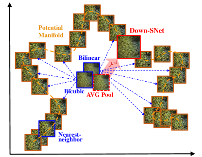
The proposed method provides a powerful Down-SNet for generating photo-realistic LR images of high perceptual quality. Down-SNet encourages the LR image to move towards regions of the potential manifold with high probability of containing photo-realistic textures. Fig. 7 shows two standard test images (lena and baboon) generated by Down-SNet compared to traditional down-sampling methods. Down-SNet generates relatively sharper and richer textures.

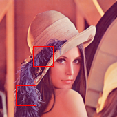
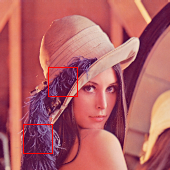
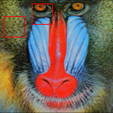
(a) Bilinear

(b) Bicubic

(c) Down-SNet

Figure 7: Reduced-resolution results with scale factor $\times 3$. Down-SNet’s result looks slightly sharper than bilinear and bicubic interpolation. (1) The first row shows the image lena. Down-SNet generates more realistic and sharper hair textures. (2) The second row shows the image baboon. Down-SNet produces high-frequency patterns missing in the bicubic and bilinear results, e.g., the fur and the light-spot in the baboon’s eyeball.

To quantitatively assess the down-sampling performance, bicubic degradation is replaced by Down-SNet to generate training samples for HR restoration. We retrain the SR networks with three types of representative architectures, including plain network (SRCNN [32]), residual network (VDSR [18]), and dense network (Up-SNet). The Down-SNet remains fixed during the optimization process. Due to useful information preserving, Down-SNet brings significant improvement for HR restoration shown in Table 3. Although the Down-SNet is trained with Up-SNet in DSN, it has excellent generalization with the other network architectures. Therefore, Down-SNet as a CNN-based down-sampling can be used to replace traditional interpolation in image processing.

Table 3: Compare average PSNR with different down-sampling degradations for $\times 3$ SR on datasets Set5 [24], Set14 [33], B100 [29] and Urban [34].

Dataset	SRCNN [32]		VDSR [18]		Up-SNet		DSN
	Bicubic	Down-SNet	Bicubic	Down-SNet	Bicubic	Down-SNet	(co-train)
Set5	32.75	33.24	33.66	33.85	33.67	33.98	34.29
Set14	29.30	29.78	29.77	29.93	29.80	30.19	30.30
B100	28.41	28.67	28.82	29.11	28.58	28.92	28.99
Urban	26.24	26.90	27.14	28.02	26.81	27.66	28.03

4.3 Image Super-Resolution Comparisons

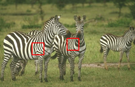
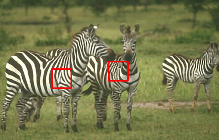
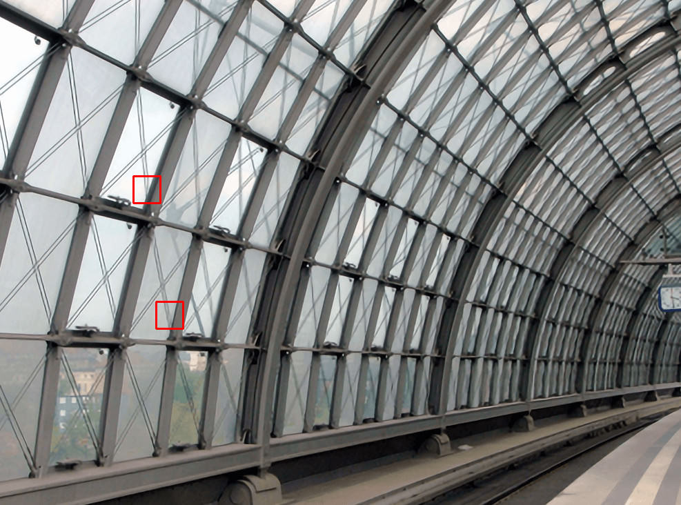
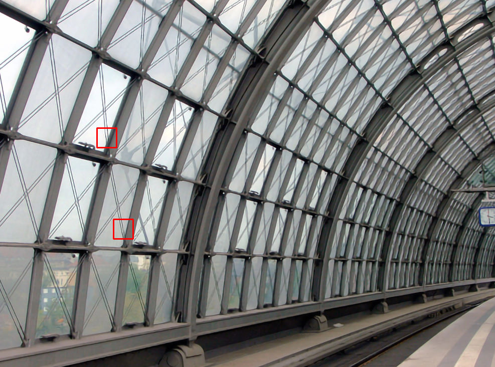
With the powerful down-sampling process, more useful information is preserved for image up-sampling. To further assess co-training DSN for SR, DSN is evaluated using three different scale factors ($\times 2$, $\times 3$, $\times 4$) on four datasets [24, 33, 29, 34]. We compute the peak signal-to-noise ratio (PSNR) and structural similarity (SSIM) to compare five recent methods including FSRCNN [16], VDSR [18], DRCN [20], DRRN [21], and MemNet [23]. As shown in Table 4, the proposed DSN outperforms the other methods. Qualitative comparisons of SRCNN [32], FSRCNN [16], and VDSR [18] are illustrated in Fig. 8 with their public codes. Our method produces relatively sharper edges and contours, while the other methods generate blurry results. In addition, existing methods produce severe distortions in some reconstructed results, whereas DSN reconstructs the texture patterns and avoids the distortions.

Table 4: Average PSNR/SSIM for scale factors $\times 2$, $\times 3$ and $\times 4$ on datasets Set5 [24], Set14 [33], B100 [29] and Urban [34]. Red indicates the best performance and blue indicates the second-best performance.

Dataset	Scale	FSRCNN [16]	VDSR [18]	DRCN [20]	DRRN [21]	MemNet [23]	DSN
Set5	$\times 2$	37.00/0.9558	37.53/0.9587	37.63/0.9588	37.74/0.9591	37.78/0.9597	37.92/0.9549
	$\times 3$	33.16/0.9140	33.66/0.9213	33.82/0.9226	34.03/0.9244	34.09/0.9248	34.29/0.9300
	$\times 4$	30.71/0.8657	31.35/0.8838	31.53/0.8854	31.68/0.8888	31.74/0.8893	31.92/0.9032
Set14	$\times 2$	32.63/0.9088	33.03/0.9124	33.04/0.9118	33.23/0.9136	33.28/0.9142	34.11/0.9286
	$\times 3$	29.43/0.8242	29.77/0.8314	29.76/0.8311	29.96/0.8349	30.00/0.8350	30.30/0.8578
	$\times 4$	27.59/0.7535	28.01/0.7674	28.02/0.7670	28.21/0.7721	28.26/0.7723	28.34/0.7539
B100	$\times 2$	31.50/0.8906	31.90/0.8960	31.85/0.8942	32.05/0.8973	32.08/0.8978	32.52/0.9074
	$\times 3$	28.52/0.7893	28.82/0.7976	28.80/0.7963	28.95/0.8004	28.96/0.8001	28.99/0.7969
	$\times 4$	26.96/0.7128	27.29/0.7251	27.23/0.7233	27.38/0.7284	27.40/0.7281	27.22/0.7010
Urban	$\times 2$	29.85/0.9009	30.76/0.9140	30.75/0.133	31.23/0.9188	31.31/0.9195	32.27/0.9305
	$\times 3$	26.42/0.8064	27.14/0.8279	27.15/0.8276	27.53/0.8378	27.56/0.8376	28.03/0.8346
	$\times 4$	24.60/0.7258	25.18/0.7524	25.14/0.7510	25.44/0.7638	25.50/0.7630	25.66/0.7145

Ground True

Bicubic

SRCNN [32]

FSRCNN [16]

VDSR [18]

DSN

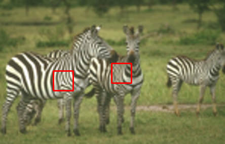
(PSNR/SSIM)

(16.82/0.3572)

(19.93/0.4999)

(19.62/0.4100)

(20.42/0.3765)

(22.44/0.7384)

(PSNR/SSIM)

(24.26/0.6997)

(26.19/0.7566)

(27.65/0.7637)

(30.27/0.7894)

(32.37/0.8266)

(PSNR/SSIM)

(23.42/0.3567)

(23.95/0.0.3961)

(23.78/0.3567)

(25.24/0.4567)

(27.92/0.9024)

Figure 8: Super-resolution results with scale factor $\times 3$ and average PSNR/SSIM of each sub-figure. (1) The first row shows image 253027 from B100 [29]. DSN accurately reconstruct the original pattern, while severe distortions are found in the results using other methods. (2) The second row shows image ppt3 from Set14 [33]. Text in DSN is sharp and identified, while others are blurry. (3) The last row shows image img002 from Urban [34]. DSN reconstructs the lines well, while other methods generate blurry results.

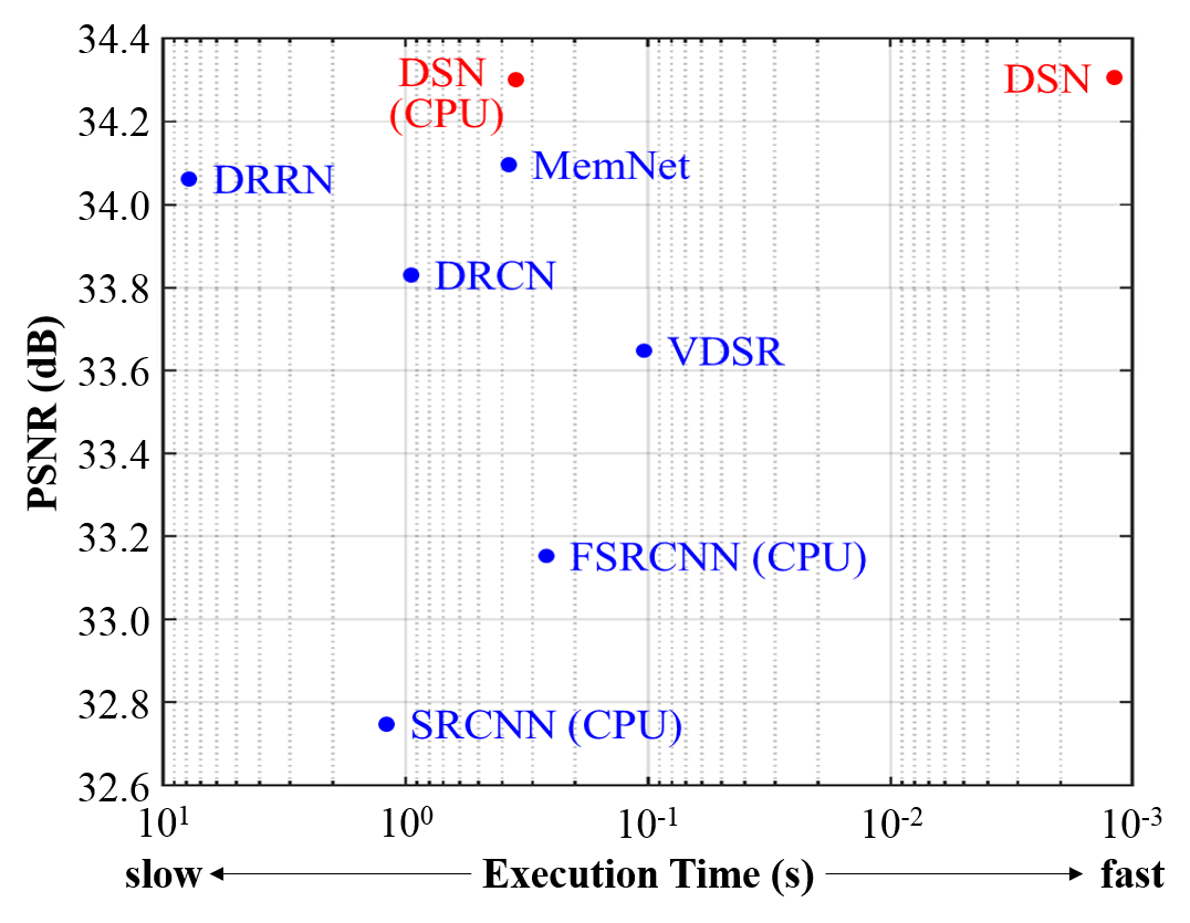
In addition, we evaluate effectiveness according to execution time using the public code of the compared methods. The experiments are conducted with an Intel CPU (Xeon E5-2620, 2.1 GHz) and an NVIDIA GPU (GeForce GTX 1080). Fig. 9 shows the PSNR of the comparator methods versus execution time. The up-sampling phase of DSN out-performs existing methods. Even on a mobile CPU platform (A9 of iPhone 6S), our method for scale factor $\times 3$ implemented with the ncnn library processes a $150\times 150$ image in approximately 200 ms. Therefore, DSN can be used to generate thumbnails and reconstruct HR images for wide mobile applications.

Figure 9: Plot of the trade-off between accuracy and speed for different methods on Set5 [24] with scale factor $\times 3$. The proposed DSN achieves better restoration quality than existing methods and is 100-times faster than MemNet [23].

4.4 Image Compression Comparisons

Image compression is a fundamental and well-studied engineering problem that aims to reduce irrelevance and redundancy for storage and transmission. With decreasing bits per pixel (bpp), high compression ratios cause blocking artifacts or noises in the decoded images. Existing image codecs usually consists of transformation, quantization, and entropy coding. Recently, deep learning-based image compression methods [35, 36] have achieved competitive performance. However, they are incompatible with existing image codecs, limiting their wideapread application in engineering. DSN is compatible with existing image coding standards to improve image compression. In DSN, Down-SNet produces a compact transformation for encoding using existing codecs, and Up-SNet reconstructs the decoded image to avoid blocking artifacts.

To evaluate the performance of DSN for image compression, we conduct experiments with standard compression methods including JPEG and JPEG2000. For compression evaluation, luminance values are usually considered in YCbCr color space. Bits for header information of compressed files count towards the bit rate of the compared methods. Since JPEG is without lossless compression, compared to JPEG, we use DSN for compression transforming and a common file compressor for quantization coding. The raw image is down-sampled by Down-SNet and stored as a .pgm file, an uncompressed format. Then, the .pgm file is coded by 7-Zip with solid compression. Compared to JPEG2000, we simply adopt OpenJPEG with lossless compression to code the LR image generated by Down-SNet.

Table 5: bpp/SSIM results of DSN + (7-Zip/JPEG2000), JPEG and JPEG2000 on dataset Set5 [24].

Image	JPEG		JPEG2000 (J2K)
	DSN + 7-Zip	JPEG ($q=44$)	DSN + J2K	J2K ($r=13\%$)
baby ($510\times 510$)	0.6051/0.9829	0.5367/0.9614	0.5189/0.9829	0.6000/0.9713
bird ($288\times 288$)	0.6726/0.9656	0.6639/0.9609	0.6012/0.9656	0.5971/0.9581
butterfly ($255\times 255$)	0.7420/0.9608	1.1448/0.9411	0.7524/0.9608	0.5878/0.9160
head ($279\times 279$)	0.6050/0.8376	0.6057/0.8082	0.5400/0.8376	0.5700/0.8470
woman ($228\times 342$)	0.6689/0.9439	0.7252/0.9326	0.6157/0.9439	0.5960/0.9436
Average	0.6587/0.9300	0.7353/0.9290	0.5800/0.9300	0.5902/0.9272

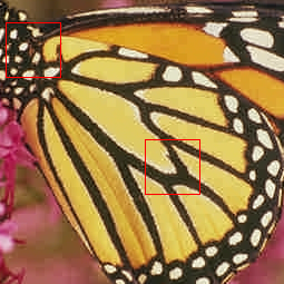
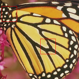
In Table 5, we evaluate the compression ratio on Set5 with a similar distortion factor SSIM. We use DSN trained with scale factor $\times 3$ as the transformation. For JPEG and JPEG2000, we test the codecs at quality parameter $q=44$ and compression ratio $r=13\%$, respectively. The comparisons show that the proposed method significantly outperforms JPEG and JPEG2000 in terms of bbp. To demonstrate the qualitative nature of compression artifacts, we show a representative example of the compressed image butterfly with $\text{bpp}\approx 0.74$ in Fig. 10.

Ground True

JPEG

JPEG2000

DSN

(bbp/SSIM)

(0.7608/0.9450)

(0.7524/0.9353)

(0.7420/0.9608)

Figure 10: Subjective comparison of JPEG, JPEG2000, and DSN with bit rate 0.74bpp. Visually disturbing blocking, aliasing, or ringing artifacts are commonly seen in images compressed with JPEG or JPEG2000. With DSN, compressed images preserves the smoothness and sharpness of many contours and edges, giving them a more natural appearance.

5 Conclusion

In image sampling, down-sampling loses useful information and up-sampling at the first layer does not provide extra information. To address these problems, hear we proposed a deep sampling network (DSN). DSN is an end-to-end system without any cheap interpolation to simultaneously learn mappings for resolution reduction and improvement. The down-sampling subnetwork in DSN can also be applied to generate photo-realistic LR images and replace traditional interpolation in image processing. Moreover, our experimental results reveal that the co-training network achieves state-of-the-art performance on SR at higher speed, and improves image compression with existing image coding standards.

References

- [1] Goto, T., Fukuoka, T., Nagashima, F., Hirano, S., Sakurai, M.: Super-resolution system for 4k-hdtv. In: Pattern Recognition (ICPR), 2014 22nd International Conference on, IEEE (2014) 4453–4458
- [2] Shi, W., Caballero, J., Ledig, C., Zhuang, X., Bai, W., Bhatia, K., de Marvao, A.M.S.M., Dawes, T., O’Regan, D., Rueckert, D.: Cardiac image super-resolution with global correspondence using multi-atlas patchmatch. In: International Conference on Medical Image Computing and Computer-Assisted Intervention, Springer (2013) 9–16
- [3] Thornton, M., Atkinson, P.M., Holland, D.: Sub-pixel mapping of rural land cover objects from fine spatial resolution satellite sensor imagery using super-resolution pixel-swapping. International Journal of Remote Sensing 27(3) (2006) 473–491
- [4] Zhang, L., Zhang, H., Shen, H., Li, P.: A super-resolution reconstruction algorithm for surveillance images. Signal Processing 90(3) (2010) 848–859
- [5] De Boor, C.: Bicubic spline interpolation. Studies in Applied Mathematics 41(1-4) (1962) 212–218
- [6] Duchon, C.E.: Lanczos filtering in one and two dimensions. Journal of Applied Meteorology 18(8) (1979) 1016–1022
- [7] Sun, J., Xu, Z., Shum, H.Y.: Image super-resolution using gradient profile prior. In: Computer Vision and Pattern Recognition, 2008. CVPR 2008. IEEE Conference on, IEEE (2008) 1–8
- [8] Glasner, D., Bagon, S., Irani, M.: Super-resolution from a single image. In: Computer Vision, 2009 IEEE 12th International Conference on, IEEE (2009) 349–356
- [9] Chang, H., Yeung, D.Y., Xiong, Y.: Super-resolution through neighbor embedding. In: Computer Vision and Pattern Recognition, 2004. CVPR 2004. Proceedings of the 2004 IEEE Computer Society Conference on. Volume 1., IEEE (2004) I–I
- [10] Yang, J., Wright, J., Huang, T.S., Ma, Y.: Image super-resolution via sparse representation. IEEE transactions on image processing 19(11) (2010) 2861–2873
- [11] Schulter, S., Leistner, C., Bischof, H.: Fast and accurate image upscaling with super-resolution forests. In: Proceedings of the IEEE Conference on Computer Vision and Pattern Recognition. (2015) 3791–3799
- [12] Simonyan, K., Zisserman, A.: Very deep convolutional networks for large-scale image recognition. arXiv preprint arXiv:1409.1556 (2014)
- [13] Girshick, R., Donahue, J., Darrell, T., Malik, J.: Rich feature hierarchies for accurate object detection and semantic segmentation. In: Proceedings of the IEEE conference on computer vision and pattern recognition. (2014) 580–587
- [14] Chen, L.C., Papandreou, G., Kokkinos, I., Murphy, K., Yuille, A.L.: Deeplab: Semantic image segmentation with deep convolutional nets, atrous convolution, and fully connected crfs. arXiv preprint arXiv:1606.00915 (2016)
- [15] Dong, C., Loy, C.C., He, K., Tang, X.: Learning a deep convolutional network for image super-resolution. In: European Conference on Computer Vision, Springer (2014) 184–199
- [16] Dong, C., Loy, C.C., Tang, X.: Accelerating the super-resolution convolutional neural network. In: European Conference on Computer Vision, Springer (2016) 391–407
- [17] Shi, W., Caballero, J., Huszár, F., Totz, J., Aitken, A.P., Bishop, R., Rueckert, D., Wang, Z.: Real-time single image and video super-resolution using an efficient sub-pixel convolutional neural network. In: Proceedings of the IEEE Conference on Computer Vision and Pattern Recognition. (2016) 1874–1883
- [18] Kim, J., Kwon Lee, J., Mu Lee, K.: Accurate image super-resolution using very deep convolutional networks. In: Proceedings of the IEEE Conference on Computer Vision and Pattern Recognition. (2016) 1646–1654
- [19] Mao, X., Shen, C., Yang, Y.B.: Image restoration using very deep convolutional encoder-decoder networks with symmetric skip connections. In: Advances in Neural Information Processing Systems. (2016) 2802–2810
- [20] Kim, J., Kwon Lee, J., Mu Lee, K.: Deeply-recursive convolutional network for image super-resolution. In: Proceedings of the IEEE Conference on Computer Vision and Pattern Recognition. (2016) 1637–1645
- [21] Tai, Y., Yang, J., Liu, X.: Image super-resolution via deep recursive residual network. In: Proceedings of the IEEE Conference on Computer Vision and Pattern Recognition. (2017)
- [22] Kingma, D., Ba, J.: Adam: A method for stochastic optimization. arXiv preprint arXiv:1412.6980 (2014)
- [23] Tai, Y., Yang, J., Liu, X., Xu, C.: Memnet: A persistent memory network for image restoration. In: Proceedings of the IEEE Conference on Computer Vision and Pattern Recognition. (2017) 4539–4547
- [24] Bevilacqua, M., Roumy, A., Guillemot, C., Alberi-Morel, M.L.: Low-complexity single-image super-resolution based on nonnegative neighbor embedding. (2012)
- [25] He, K., Zhang, X., Ren, S., Sun, J.: Deep residual learning for image recognition. In: Proceedings of the IEEE conference on computer vision and pattern recognition. (2016) 770–778
- [26] Cai, B., Xu, X., Jia, K., Qing, C., Tao, D.: Dehazenet: An end-to-end system for single image haze removal. IEEE Transactions on Image Processing 25(11) (2016) 5187–5198
- [27] Huang, G., Liu, Z., Weinberger, K.Q., van der Maaten, L.: Densely connected convolutional networks. arXiv preprint arXiv:1608.06993 (2016)
- [28] Szegedy, C., Vanhoucke, V., Ioffe, S., Shlens, J., Wojna, Z.: Rethinking the inception architecture for computer vision. In: Proceedings of the IEEE Conference on Computer Vision and Pattern Recognition. (2016) 2818–2826
- [29] Martin, D., Fowlkes, C., Tal, D., Malik, J.: A database of human segmented natural images and its application to evaluating segmentation algorithms and measuring ecological statistics. In: Computer Vision, 2001. ICCV 2001. Proceedings. Eighth IEEE International Conference on. Volume 2., IEEE (2001) 416–423
- [30] He, K., Zhang, X., Ren, S., Sun, J.: Delving deep into rectifiers: Surpassing human-level performance on imagenet classification. In: Proceedings of the IEEE international conference on computer vision. (2015) 1026–1034
- [31] Jia, Y., Shelhamer, E., Donahue, J., Karayev, S., Long, J., Girshick, R., Guadarrama, S., Darrell, T.: Caffe: Convolutional architecture for fast feature embedding. In: Proceedings of the 22nd ACM international conference on Multimedia, ACM (2014) 675–678
- [32] Dong, C., Loy, C.C., He, K., Tang, X.: Image super-resolution using deep convolutional networks. IEEE transactions on pattern analysis and machine intelligence 38(2) (2016) 295–307
- [33] Zeyde, R., Elad, M., Protter, M.: On single image scale-up using sparse-representations. In: International conference on curves and surfaces, Springer (2010) 711–730
- [34] Huang, J.B., Singh, A., Ahuja, N.: Single image super-resolution from transformed self-exemplars. In: Proceedings of the IEEE Conference on Computer Vision and Pattern Recognition. (2015) 5197–5206
- [35] Theis, L., Shi, W., Cunningham, A., Huszár, F.: Lossy image compression with compressive autoencoders. arXiv preprint arXiv:1703.00395 (2017)
- [36] Ballé, J., Laparra, V., Simoncelli, E.P.: End-to-end optimized image compression. arXiv preprint arXiv:1611.01704 (2016)