A general formulation of long-range degree correlations in complex networks

Abstract

We provide a general framework for analyzing degree correlations between nodes separated by more than one step (i.e., beyond nearest neighbors) in complex networks. One probability and four conditional probabilities are introduced to fully describe long-range degree correlations with respect to $k$ and $k^{\prime}$ of two nodes and shortest path length $l$ between them. We present general relations among these probabilities and clarify the relevance to nearest-neighbor degree correlations. Unlike nearest-neighbor correlations, some of these probabilities are meaningful only in finite-size networks. Furthermore, as a baseline to determine the existence or nonexistence of long-range degree correlations in a network, the functional forms of these probabilities for networks without any long-range degree correlations are analytically evaluated within a mean-field approximation. The validity of our argument is demonstrated by applying it to real-world networks.

I Introduction

In many networks describing complex real systems, the number of edges from a node, namely degree, widely fluctuates from node to node, and degree distributions often exhibit power-law behavior Barabasi99 . For such networks, significant interest now concentrates on the issue of correlations between degrees of two nodes. In particular, degree correlations between adjacent nodes have been extensively studied so far Pastor-Satorras01 ; Maslov02 ; Newman02 ; Newman03 ; Park03 ; Catanzaro04 ; Serrano06 ; Fotouhi13 ; Litvak13 . Nearest neighbor degree correlations (NNDCs) in complex networks are related to their fundamental structural properties, such as clustering Soffer05 ; Serrano05 ; Miller09 ; Hofstad17 , community structures Menche10 , the average path length Xulvi-Brunet04 , and fractality Yook05 ; Song06 ; Wei16 . In addition, NNDCs influence various dynamics on networks, such as epidemic spreading Eguiluz02 ; Boguna02 ; Boguna03 ; Gross06 ; Hindes17 , synchronization phenomena Sorrentino06 ; Bernardo07 ; LaMar10 ; LaRocca11 ; Avalos-Gaytan12 ; Jalan16 , strategic games Rong07 ; Rong09 ; Devlin09 ; La17 , and resilience to failures Noh07 ; Goltsev08 ; Schneider11 ; Tanizawa12 ; Watanabe16 .

It has, however, been pointed out recently that NNDCs are not enough to characterize structural properties of complex networks. For example, scale-free fractal networks are known to exhibit negative NNDCs (namely, disassortative mixing) Yook05 . Thus, hub nodes in such a network are almost never connected directly by an edge. In actual fractal networks, like the World Wide Web or synthetic graphs Song06 ; Rozenfeld07 , however, hub nodes are not only nonadjacent to, but also repulsive over a long-range distance to each other Fujiki17 . As another example, Orsini et al. Orsini15 found that many local and even global structural features of real-world complex networks are closely reproduced by random graphs with the same degree sequences, clustering, and NNDCs as those for the real networks. However, some sort of global properties, such as the shortest path length distributions, betweenness distributions, and community structures, cannot be explained by these local characteristics. This implies that intrinsic non-local degree correlations in these networks cannot be described by NNDCs as a local characteristic. Furthermore, it has been demonstrated that the shortest path length between hub nodes influences functions or dynamical properties of networks Tadic04 ; Boguna13 ; Boulos13 ; Swanson16 . For understanding non-local structural properties, it is important and useful to provide a framework to describe degree correlations between nodes beyond nearest neighbors, namely, long-range degree correlations (LRDCs).

There have been several proposals for formulating LRDCs in complex networks. Rybski et al. Rybski10 describe LRDCs by fluctuations of the degree along shortest paths between two nodes. This is an analogy to fluctuation analysis used in correlated time series. Mayo et al. Mayo15 defined the long-range assortativity and the average $l$th neighbor degree to quantify LRDCs (the same definition of the long-range assortativity was independently employed in Arcagni17 ). The long-range assortativity $r_{l}$ is the Pearson correlation coefficient between degrees of pairs of nodes separated by the shortest path length $l$ from each other. The average $l$th neighbor degree $k_{l}(k)$ is the average degree of nodes separated by $l$ from a node of degree $k$. They found that social networks exhibit disassortative degree correlations on long-range scales, while nonsocial networks do not indicate such a tendency. The two-walks degree assortativity proposed by Allen-Perkins et al. Allen-Perkins17 is another type of assortativity measure beyond nearest neighbors. This quantity is defined as the Pearson correlation coefficient of the sum of the nearest-neighbor degrees of adjacent nodes, which reflects second neighbor degree correlations. These quantities enable us to pick up some specific aspects of LRDCs. However, if we perform a global and multilateral analysis of LRDCs, a more general framework is required to obtain the entire information of LRDCs.

In this work, we provide a general framework for analyzing LRDCs in complex networks of either finite or infinite size. In order to fully describe correlations between degrees $k$ and $k^{\prime}$ of two nodes separated by a shortest path length $l$, one joint probability and four conditional probabilities are introduced as functions of $k$, $k^{\prime}$, and $l$. NNDCs can be described by these probability functions as a special case of $l=1$. These five probabilities are not independent of each other, and we present general relations among them. In addition, the functional forms of these probabilities for a network without any LRDCs (referred as a long-range uncorrelated network hereafter) are analytically evaluated within a mean-field approximation. By comparing the probabilities for a given network with those for the corresponding long-range uncorrelated network, one can judge whether the network possesses LRDCs or not, and obtain detailed information about degree correlations. Finally, we demonstrate the validity of our argument by applying it to real-world networks.

The rest of this paper is organized as follows. In Sec. II, we introduce the probability functions characterizing LRDCs and present general relations between them. In Sec. III, the functional forms of the probabilities for long-range uncorrelated networks are analytically evaluated. In Sec. IV, the validity of our argument is tested by calculating the probabilities for real-world networks. Section V is devoted to the summary and remarks.

II Joint and conditional probabilities

Degree correlations between nearest-neighbor nodes (namely, NNDCs) are completely described by the joint probability $P_{\text{nn}}(k,k^{\prime})$ that two end nodes of a randomly chosen edge have the degrees $k$ and $k^{\prime}$. We can define the conditional probability from $P_{\text{nn}}(k,k^{\prime})$ by $P_{\text{nn}}(k^{\prime}|k)=P_{\text{nn}}(k,k^{\prime})/\sum_{k^{\prime}}P_{\text{nn}}(k,k^{\prime})$, which is the probability that a node adjacent to a randomly chosen node of degree $k$ has the degree $k^{\prime}$. If the degree distribution function $P(k)$ is given, the probability $P_{\text{nn}}(k^{\prime}|k)$ also identifies NNDCs. We extend this idea to LRDCs. All information pertaining to correlations between degrees $k$ and $k^{\prime}$ of two nodes separated by a shortest path length $l$ (namely, LRDCs) is included in the joint probability $P(k,k^{\prime},l)$ that randomly chosen two nodes have the degrees $k$ and $k^{\prime}$ and the shortest path length between them is $l$. From this joint probability, four conditional probabilities can be constructed as follows,

$$P(l|k,k^{\prime}) = \frac{P(k,k^{\prime},l)}{\sum_{l}P(k,k^{\prime},l)},$$ (1a)

$$P(k^{\prime}|k,l) = \frac{P(k,k^{\prime},l)}{\sum_{k^{\prime}}P(k,k^{\prime},l)},$$ (1b)

$$P(k,k^{\prime}|l) = \frac{P(k,k^{\prime},l)}{\sum_{k,k^{\prime}}P(k,k^{\prime},l)},$$ (1c)

$$P(k^{\prime},l|k) = \frac{P(k,k^{\prime},l)}{\sum_{k^{\prime},l}P(k,k^{\prime},l)}.$$ (1d)

The meanings of these probabilities, as well as the joint probability, are listed in Table 1. These conditional probabilities also describe LRDCs. The probabilities in Table 1 are normalized as $\sum_{k,k^{\prime},l}P(k,k^{\prime},l)=\sum_{l}P(l|k,k^{\prime})=\sum_{k^{\prime}}P(k^{\prime}|k,l)=\sum_{k,k^{\prime}}P(k,k^{\prime}|l)=\sum_{k^{\prime},l}P(k^{\prime},l|k)=1$. Here, we note that the sum over $l$ includes the distance ($l_{\infty}$) between disconnected node pair. It should be also emphasized that $P(k,k^{\prime},l)$, $P(l|k,k^{\prime})$, and $P(k^{\prime},l|k)$ are meaningless for networks with infinitely large components because values of these probabilities become always zero for finite $l$. In contrast, $P(k^{\prime}|k,l)$ and $P(k,k^{\prime}|l)$ can be properly defined even for infinite networks.

Table 1: Meanings of one joint probability and four conditional probabilities characterizing LRDCs in networks.

Probability	Meaning
$P(k,k^{\prime},l)$	Probability that randomly chosen two nodes have the degrees $k$ and $k^{\prime}$ and the distance between them is $l$
$P(l|k,k^{\prime})$	Probability that randomly chosen two nodes of degrees $k$ and $k^{\prime}$ are separated by $l$, namely, the shortest path length distribution between nodes of degrees $k$ and $k^{\prime}$
$P(k^{\prime}|k,l)$	Probability that a node separated by $l$ from a randomly chosen node of degree $k$ has the degree $k^{\prime}$, namely, the degree distribution of a node separated by $l$ from a node of degree $k$
$P(k,k^{\prime}|l)$	Probability that randomly chosen two nodes separated by $l$ from each other have the degrees $k$ and $k^{\prime}$
$P(k^{\prime},l|k)$	Probability that a randomly chosen node has the degree $k^{\prime}$ and is separated by $l$ from a node of degree $k$

Using the joint probability $P(k,k^{\prime},l)$, the degree distribution $P(k)$ and the shortest path length distribution $R(l)$ are presented by

$$P(k)=\sum_{k^{\prime},l}P(k,k^{\prime},l),$$ (2)

and

$$R(l)=\sum_{k,k^{\prime}}P(k,k^{\prime},l),$$ (3)

respectively. It is convenient to introduce the probability $Q(k|l)$ defined by

$$Q(k|l)=\sum_{k^{\prime}}P(k,k^{\prime}|l),$$ (4)

which is the probability that one of two nodes separated by $l$ has the degree $k$. This is an extension of the probability $Q_{\text{nn}}(k)$ that one end node of an edge has the degree $k$ to a long-range node pair in the sense of $Q_{\text{nn}}(k)=Q(k|l=1)$. With the aid of $Q(k|l)$, we have

$$\sum_{k^{\prime}}P(k,k^{\prime},l)=Q(k|l)R(l).$$ (5)

Equations (2), (3), and (5), as well as the obvious relation

$$\sum_{l}P(k,k^{\prime},l)=P(k)P(k^{\prime}),$$ (6)

form sum rules of the joint probability $P(k,k^{\prime},l)$. Considering these sum rules, Eq. (1) leads several general relations between the conditional probabilities, $P(k)$, and $R(l)$, such as,

$$P(k^{\prime},l|k)=P(k^{\prime})P(l|k,k^{\prime}),$$ (7)

$$P(k,k^{\prime}|l)=Q(k|l)P(k^{\prime}|k,l),$$ (8)

$$P(k)P(k^{\prime},l|k)=Q(k^{\prime}|l)R(l)P(k|k^{\prime},l),$$ (9)

and

$$P(k)P(k^{\prime})P(l|k,k^{\prime})=R(l)P(k,k^{\prime}|l).$$ (10)

Equations (9) and (10) can be considered as direct consequences of the Bayes’ theorem that relates $P(A|B)$ and $P(B|A)$ for events $A$ and $B$.

The joint probability $P_{\text{nn}}(k,k^{\prime})$ and the conditional probability $P_{\text{nn}}(k^{\prime}|k)$ describing NNDCs are included in the above long-range probabilities as a special case of $l=1$. In fact, we have

$$P_{\text{nn}}(k,k^{\prime})=P(k,k^{\prime}|l=1),$$ (11)

and

$$P_{\text{nn}}(k^{\prime}|k)=P(k^{\prime}|k,l=1).$$ (12)

Similarly, the degree distribution $Q_{\text{nn}}(k)$ of an end node of a randomly chosen edge is given by

$$Q_{\text{nn}}(k)=Q(k|l=1)=\frac{kP(k)}{\langle k\rangle},$$ (13)

where $\langle k\rangle=\sum_{k}kP(k)$ is the average degree. Then, Eq. (8) with $l=1$ is reduced to the well-known relation $P_{\text{nn}}(k,k^{\prime})=kP(k)P_{\text{nn}}(k^{\prime}|k)/\langle k\rangle$ Boguna02 .

Considering the above correspondence, we can easily extend indices characterizing NNDCs to those for LRDCs. For example, the long-range assortativity $r_{l}$ can be defined as

$$r_{l}=\frac{4\langle kk^{\prime}\rangle_{l}-\langle k+k^{\prime}\rangle_{l}^{2}}{2\langle k^{2}+k^{\prime 2}\rangle_{l}-\langle k+k^{\prime}\rangle_{l}^{2}},$$ (14)

where $\langle f(k,k^{\prime})\rangle_{l}=\sum_{k,k^{\prime}}f(k,k^{\prime})P(k,k^{\prime}|l)$. This quantity is the Pearson correlation coefficient between degrees of nodes separated by $l$ from each other. For $l=1$, $r_{l}$ is reduced to the conventional nearest-neighbor assortativityNewman02 . Another example is the average degree of $l$th neighbor nodes, which is given by comment1

$$k_{l}(k)=\sum_{k^{\prime}}k^{\prime}P(k^{\prime}|k,l).$$ (15)

This is an extension of the average degree, $k_{\text{nn}}(k)=\sum_{k^{\prime}}k^{\prime}P_{\text{nn}}(k^{\prime}|k)$, of nearest neighbors of a node of degree $k$ to that for $l$th neighbors. The quantities $r_{l}$ and $k_{l}(k)$ are equivalent to those proposed by Ref. Mayo15 . Besides extensions of existing indices for NNDCs, it is also possible to introduce completely new measures characterizing LRDCs, such as the strength of long-range repulsive correlations between hubs, by using the probabilities listed in Table 1.

III Long-range uncorrelated networks

In the previous section, we introduced five fundamental probabilities describing LRDCs in complex networks. However, even if we know these probabilities for a given network, we cannot judge whether the network possesses LRDCs or not. This is due to the lack of a baseline for comparison, i.e., it has not yet been clarified how these probabilities behave for a network in which the degrees of two nodes separated by an arbitrary distance are not correlated. In this section, we evaluate functional forms of the probabilities for long-range uncorrelated networks (LRUNs).

III.1 General remarks

A nearest-neighbor uncorrelated network (NNUN) is a network in which the degree of one end node of an edge is independent of the degree of another end node. Thus, the joint probability $P_{\text{nn}}(k,k^{\prime})$ in an NNUN is given by the product $Q_{\text{nn}}(k)Q_{\text{nn}}(k^{\prime})$. Extending this idea, an LRUN is considered to be a network satisfying the relation

$$P_{0}(k,k^{\prime}|l)=Q_{0}(k|l)Q_{0}(k^{\prime}|l),$$ (16)

for any $l$, where $P_{0}(k,k^{\prime}|l)$ and $Q_{0}(k|l)$ represent $P(k,k^{\prime}|l)$ and $Q(k|l)$ for LRUNs, respectively. Hereafter, we denote the probabilities for LRUNs by adding the subscript “$0$”. Equation (16) implies that the degrees $k$ and $k^{\prime}$ of two nodes separated by $l$ are independent of each other.

While $P_{\text{nn}}(k,k^{\prime})$ for an NNUN has the simple functional form as $P_{\text{nn}}(k,k^{\prime})=kk^{\prime}P(k)P(k^{\prime})/\langle k\rangle^{2}$, it is difficult to obtain an exact expression of $P_{0}(k,k^{\prime}|l)$ because $Q(k|l)$ itself depends on LRDCs. Nevertheless, we can generally conclude that $P_{0}(k^{\prime}|k,l)$ for an LRUN does not depend on $k$. This comes immediately from the relation

$$P_{0}(k^{\prime}|k,l)=Q_{0}(k^{\prime}|l),$$ (17)

which is obtained by substituting Eq. (16) into Eq. (8). Equation (17) with $l=1$ leads the well-known relation $P_{\text{nn}}(k^{\prime}|k)=k^{\prime}P(k^{\prime})/\langle k\rangle$ for NNUNs Boguna02 .

III.2 Mean-field approximation

We have mentioned that the probability functions for LRUNs are not easy to calculate rigorously. A major reason for this difficulty is that finite sizes of networks are essential for these probabilities, as pointed out in Sec. II. Thus, we need to approximate these probabilities for LRUNs. Once one of these probabilities is obtained, other probabilities can be calculated by using Eq. (1). We then focus on $P_{0}(l|k,k^{\prime})$ at first, which is the length distribution between nodes of degrees $k$ and $k^{\prime}$ and has been argued recently by Melnik and Gleeson Melnik16 . They calculated $P(l|k,k^{\prime})$ for finite random networks such as Erdős-Rényi random graphs or networks generated by the configuration model Newman01 . We can reasonably assume that finite random networks belong to the class of LRUNs when their sizes are finite but sufficiently large, from the fact that infinite random networks satisfy Eq. (16) to be LRUNs. Therefore, we take $P(l|k,k^{\prime})$ in their calculation Melnik16 as $P_{0}(l|k,k^{\prime})$ for LRUNs, after some necessary modifications comment2 .

Let us introduce the probability $\rho(l|k,k^{\prime})$ that the distance between randomly chosen two nodes of degrees $k$ and $k^{\prime}$ is equal to or less than $l$. The probability $P_{0}(l|k,k^{\prime})$ is then presented by

$$P_{0}(l|k,k^{\prime})=\begin{cases}\rho(0|k,k^{\prime})&(l=0),\\[3.0pt] \rho(l|k,k^{\prime})-\rho(l-1|k,k^{\prime})&(l\geq 1),\\[3.0pt] 1-\displaystyle\lim_{l\to\infty}\rho(l|k,k^{\prime})&(l=l_{\infty}).\end{cases}$$ (18)

The last expression for $l=l_{\infty}$ is for disconnected node pairs in a network composed of multiple components. The normalization condition of $P(l|k,k^{\prime})$ is thus written as $\sum_{l=0}^{\infty}P(l|k,k^{\prime})+P(l_{\infty}|k,k^{\prime})=1$.

Under the local tree assumption and the mean-field approximation, $\rho(l|k,k^{\prime})$ for a random network is given by Melnik16

$$\rho(l|k,k^{\prime})=1-\left[1-\rho(0|k,k^{\prime})\right]\left[1-\bar{q}(l-1|k,k^{\prime})\right]^{k},$$ (19)

where $\bar{q}(l|k,k^{\prime})$ is the probability that an adjacent node of a randomly chosen node $i_{k}$ of degree $k$ lies within the distance $l$ from a node $j_{k^{\prime}}$ of degree $k^{\prime}$ under the condition that $i_{k}$ is separated by more than $l$ from $j_{k^{\prime}}$. The first factor $1-\rho(0|k,k^{\prime})$ of the second term in the right-hand side represents the probability that the node $i_{k}$ is not the node $j_{k^{\prime}}$ itself. The second factor $\left[1-\bar{q}(l-1|k,k^{\prime})\right]^{k}$ means the probability that all adjacent nodes of $i_{k}$ are separated by more than $l-1$ from $j_{k^{\prime}}$ under the condition that $i_{k}$ is separated by more than $l-1$ from $j_{k^{\prime}}$. Thus, the rough meaning of Eq. (19) is that the probability that the node $i_{k}$ lies within the distance $l$ from the node $j_{k^{\prime}}$ is equal to the probability that at least one of $k$ adjacent nodes of $i_{k}$ lies within the distance $l-1$ from $j_{k^{\prime}}$. Furthermore, let us introduce the probability $q(l|k,k^{\prime})$ that a randomly chosen node $i_{k}$ of degree $k$ with at least one neighboring node, say $h$, separated by more than $l$ from a node $j_{k^{\prime}}$ of degree $k^{\prime}$ lies within the distance $l$. Then, we have the following relation between $q(l|k,k^{\prime})$ and $\bar{q}(l-1|k,k^{\prime})$ similar to Eq. (19),

$$q(l|k,k^{\prime})=1-\left[1-\rho(0|k,k^{\prime})\right]\left[1-\bar{q}(l-1|k,k^{\prime})\right]^{k-1}.$$ (20)

The right-hand side of this equation implies the probability that at least one node of $k-1$ adjacent nodes of $i_{k}$ other than $h$ lies within the distance $l-1$ from $j_{k^{\prime}}$. Using $q(l|k,k^{\prime})$, the probability $\bar{q}(l|k,k^{\prime})$ is expressed by

$$\bar{q}(l|k,k^{\prime}) = \sum_{k^{\prime\prime}}P_{\text{nn}}(k^{\prime\prime}|k)q(l|k^{\prime\prime},k^{\prime}),$$ (21)

$$= \frac{1}{\langle k\rangle}\sum_{k^{\prime\prime}}k^{\prime\prime}P(k^{\prime\prime})q(l|k^{\prime\prime},k^{\prime}).$$

Since $\bar{q}(l|k,k^{\prime})$ is actually independent of $k$, we denote it simply by $\bar{q}(l|k^{\prime})$. Multiplying $kP(k)/\langle k\rangle$ on both sides of Eq. (20), summing over $k$, and using Eq. (21), we have the recursion equation for $\bar{q}(l|k^{\prime})$,

$$\bar{q}(l|k^{\prime})=1 - G_{1}\left[1-\bar{q}(l-1|k^{\prime})\right]$$ (22)

$$+ \frac{k^{\prime}}{N\langle k\rangle}\left[1-\bar{q}(l-1|k^{\prime})\right]^{k^{\prime}-1},$$

where $N$ is the number of nodes in the network and $G_{1}(x)$ is the generating function defined by $G_{1}(x)=\sum_{k}x^{k-1}kP(k)/\langle k\rangle$. Here, we used the obvious relation,

$$\rho(0|k,k^{\prime})=\frac{\delta_{kk^{\prime}}}{NP(k)}.$$ (23)

Equation (22) can be solved iteratively with the initial condition Melnik16 ,

$$\bar{q}(0|k^{\prime})=\frac{k^{\prime}}{N\langle k\rangle}.$$ (24)

Using the solution of $\bar{q}(l|k^{\prime})$ and Eqs. (18) and (19), we can calculate $P_{0}(l|k,k^{\prime})$. The joint probability $P_{0}(k,k^{\prime},l)$ is computed by $P(k)P(k^{\prime})P_{0}(l|k,k^{\prime})$ from Eqs. (1a) and (6), and other conditional probabilities listed in Table 1 are determined from $P_{0}(k,k^{\prime},l)$ by using Eq. (1).

We should remark the accuracy of the mean-field approximation in the above calculation. The probability $\rho(l|k,k^{\prime})$ must be equal to $\rho(l|k^{\prime},k)$ from the definition. However, $\rho(l|k,k^{\prime})$ calculated from Eq. (19) is actually not symmetric with respect to $k$ and $k^{\prime}$. In fact, $\rho(l|k,k^{\prime})$ for $l=1$ and $k\neq k^{\prime}$, calculated as

$$\rho(1|k,k^{\prime}) = 1-\left(1-\frac{k^{\prime}}{N\langle k\rangle}\right)^{k}$$ (25)

$$= \frac{kk^{\prime}}{N\langle k\rangle}-\frac{1}{2}\frac{k(k-1)k^{\prime 2}}{\left(N\langle k\rangle\right)^{2}}+\cdots,$$

is asymmetric in the order of $N^{-2}$. This is due to the difference in accuracy of the mean-field treatment for nearest neighbors of the nodes of degrees $k$ and $k^{\prime}$. The mean-field approximation for neighboring nodes of a large degree node is more accurate than that of a small degree node. Since $\bar{q}(l|k^{\prime})$ is iteratively calculated for the distance $l$ from the source node of degree $k^{\prime}$ according to Eq. (22), $\rho(l|k,k^{\prime})$ with $k<k^{\prime}$ is more accurate than $\rho(l|k^{\prime},k)$. Therefore, we first calculate $\rho(l|k,k^{\prime})$ for $k<k^{\prime}$ by Eq. (19), then transfer it to $\rho(l|k^{\prime},k)$ in actual computations. Another remark on the mean-field approximation is related to the component-size distribution. We assume that $\rho(l|k,k^{\prime})$ does not depend on the size of the component that the source node of degree $k^{\prime}$ belongs to. This implies that the distribution function of the component size is assumed to be relatively narrow. If a random network with a given degree distribution $P(k)$ is very close to its percolation transition point, however, the component-size distribution becomes wide, and then the mean-field calculations have poor accuracy.

III.3 Infinite tree-like networks

For infinitely large networks, only $P(k^{\prime}|k,l)$ and $P(k,k^{\prime}|l)$ are meaningful among five probabilities, as mentioned in Sec. II. It is easy to calculate these conditional probabilities for infinite random networks with tree-like structures. Let us consider $P_{0}(k^{\prime}|k,l)$ at first. Since this is the probability that a node separated by $l$ from a node of degree $k$ has the degree $k^{\prime}$, $P_{0}(k^{\prime}|k,l)$ must satisfy the relation,

$$P_{0}(k^{\prime}|k,l)=\sum_{k^{\prime\prime}}P_{\text{nn}}(k^{\prime}|k^{\prime\prime})P_{0}(k^{\prime\prime}|k,l-1),$$ (26)

where the nearest-neighbor degree distribution function $P_{\text{nn}}(k^{\prime}|k^{\prime\prime})$ is given by $k^{\prime}P(k^{\prime})/\langle k\rangle$ for random networks. Using the obvious relation $P_{0}(k^{\prime}|k,0)=\delta_{kk^{\prime}}$, we can solve the above equation as,

$$P_{0}(k^{\prime}|k,l)=\begin{cases}\delta_{kk^{\prime}}&(l=0),\\[5.0pt] \displaystyle\frac{k^{\prime}P(k^{\prime})}{\langle k\rangle}&(l\geq 1).\end{cases}$$ (27)

Thus, we have immediately, from Eq. (17),

$$Q_{0}(k|l)=\frac{kP(k)}{\langle k\rangle}\quad(l\geq 1).$$ (28)

The probability $P_{0}(k,k^{\prime}|l)$ for $l\geq 1$ is then calculated from Eq. (8) as

$$P_{0}(k,k^{\prime}|l)=\frac{kk^{\prime}P(k)P(k^{\prime})}{\langle k\rangle^{2}}.$$ (29)

We should note that $P_{0}(k,k^{\prime}|l)$ and $P_{0}(k^{\prime}|k,l)$ for infinite tree-like random networks are equivalent to $P_{\text{nn}}(k,k^{\prime})$ and $P_{\text{nn}}(k^{\prime}|k)$, respectively, independently of $l$.

It is reasonable to consider that the above expressions of $P_{0}(k^{\prime}|k,l)$, $Q_{0}(k|l)$, and $P_{0}(k,k^{\prime}|l)$ for infinitely large networks hold approximately for $l\ll\langle l\rangle$ even in finite random networks, where $\langle l\rangle$ is the average shortest path length. While we have shown in Sec. III.1 that $P_{0}(k^{\prime}|k,l)$, in general, does not depend on $k$, our result here indicates that this probability is independent of $l$ too if $l\ll\langle l\rangle$.

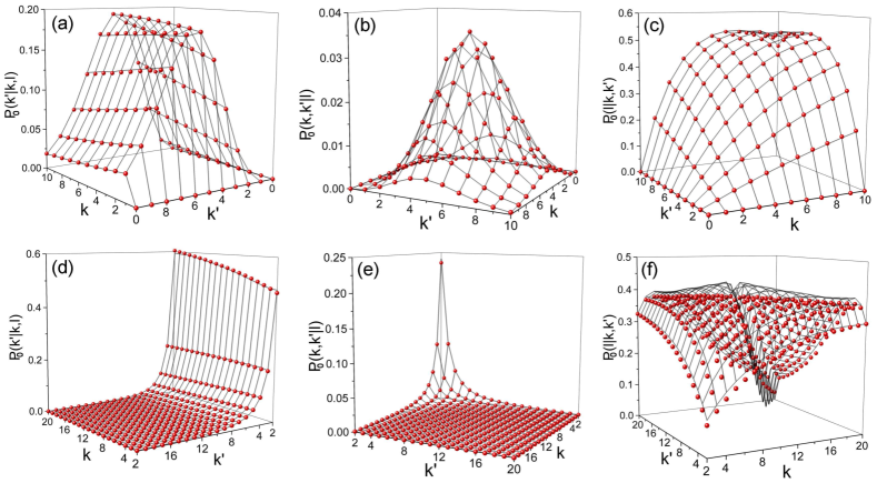
Figure 1: (Color online) Probabilities $P_{0}(k^{\prime}|k,l)$, $P_{0}(k,k^{\prime}|l)$, and $P_{0}(l|k,k^{\prime})$ as functions of $k$ and $k^{\prime}$ for $l=4$ and $N=1,000$. Wireframes indicate the probabilities calculated analytically by the method explained in Sec. III.2, while dots represent those measured for numerically realized random networks. Upper three panels [(a)-(c)] are the results for Erdős-Rényi random graphs with $\langle k\rangle=5.0$, and lower panels [(d)-(f)] for scale-free random networks with the degree distribution $P(k)\propto k^{-3}$.

III.4 Numerical confirmation

In order to confirm the validity of our analytical evaluation of the probability functions for LRUNs, we compare the probabilities $P_{0}(l|k,k^{\prime})$, $P_{0}(k^{\prime}|k,l)$, and $P_{0}(k,k^{\prime}|l)$ obtained by the method explained in Sec. III.2 with those measured for synthetic random networks. Figure 1 shows the dependence of these probabilities on $k$ and $k^{\prime}$ for $l=4$. The wireframe in each panel indicates the analytically calculated probabilities, while dots represent numerical results. The upper three panels give the results for Erdős-Rényi random graphs with $\langle k\rangle=5.0$ and $N=1,000$. We have dared to employ relatively small networks to check the validity of the method for finite sizes. Numerical results are obtained by averaging over $100$ realizations of Erdős-Rényi random graphs. The average path length of these networks is $\langle l\rangle=4.5$. The lower three panels present the results for scale-free random networks with $N=1,000$ and the degree distribution function of $P(k)\propto k^{-3}$ for $2\leq k\leq 50$ and $P(k)=0$ otherwise. Numerical results show the averages over $10,000$ realizations generated by the configuration model. The average degree and the average path length are $\langle k\rangle=3.1$ and $\langle l\rangle=5.4$, respectively. These plots demonstrate that the analytical treatment based on the mean-field approximation well reproduces numerical results even for finite networks.

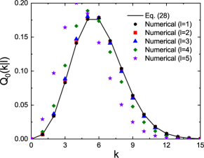
Figure 2: (Color online) Probability $Q_{0}(k|l)$ as a function of $k$ for Erdős-Rényi random graphs with $N=1,000$ and $\langle k\rangle=5.0$. Solid line indicates the probability given by Eq. (28), while symbols represent the numerical results for $l=1$ (circles), $2$ (boxes),$3$ (triangles), $4$ (diamonds), and $5$ (stars) averaged over $100$ network realizations.

We also verified the argument in Sec. III.3 by calculating $Q_{0}(k|l)$ for Erdős-Rényi random graphs. Figure 2 compares this probability calculated by Eq. (28) with $Q_{0}(k|l)$ measured numerically. The Erdős-Rényi random graphs are the same as in Fig. 1. Thus, the average path length is $\langle l\rangle=4.5$ for these random graphs. As shown by the numerical results for $l=1$, $2$, and $3$, $Q_{0}(k|l)$ measured numerically is almost independent of $l$ and is well described by Eq. (28), if $l$ is sufficiently smaller than $\langle l\rangle$. On the contrary, if $l$ becomes close to or larger than $\langle l\rangle$, numerically computed $Q_{0}(k|l)$ deviates from Eq. (28), as shown by the results for $l=4$ and $5$. These results prove that Eq. (28) holds for $l\ll\langle l\rangle$ even in finite networks.

IV Real-world networks

Finally, we investigate LRDCs in two real-world complex networks by using the probabilities listed in Table 1. One is the Gnutella peer-to-peer network gnutella and the other is the coauthorship network coauthorship . The Gnutella network has $N=10,876$ nodes and $E=39,994$ edges. Thus, the average degree is $\langle{k}\rangle=7.4$. This network consists of a single connected component. The average path length $\langle l\rangle$ and the maximum shortest path length (diameter) $l_{\text{max}}$ are $4.6$ and $10$, respectively. The Spearman’s degree-rank correlation coefficient $\rho$ Litvak13 ; Zhang16 characterizing the NNDC is measured as $\rho=0.0$, which implies no NNDC in the Gnutella network. The coauthorship network possesses $N=23,133$ nodes and $E=93,439$ edges, which give $\langle k\rangle=8.1$. This network is composed of the largest connected component with $21,363$ nodes and $566$ small components with $3.1$ nodes on average. The average path length and the network diameter are $\langle l\rangle=5.4$ and $l_{\text{max}}=15$, respectively. The Spearman’s correlation coefficient of the coauthorship network is $\rho=0.26$, which means a positive NNDC.

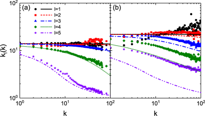
Figure 3: (Color online) Average $l$th neighbor degree $k_{l}(k)$ of a typical node of degree $k$ for (a) the Gnutella network gnutella and (b) the coauthorship network coauthorship . Symbols represent $k_{l}(k)$ of the real-world networks as a function of $k$ at fixed values of $l$, and curves indicate those of corresponding LRUNs with the same degree sequences as the real networks.

For these two real-world networks, we first calculate the average $l$th neighbor degree $k_{l}(k)$ given by Eq. (15). The results are presented by symbols in Fig. 3. The continuous curves in this figure indicate $k_{l}(k)$ for LRUNs with the same degree sequences as the real networks, which is calculated from Eq. (15) by replacing $P(k^{\prime}|k,l)$ with $P_{0}(k^{\prime}|k,l)$. The symbols for various $l$ in Fig. 3(a) are approximately fitted by the corresponding curves. This implies that the Gnutella network has almost no LRDCs. On the contrary, $k_{l}(k)$ for the coauthorship network [Fig. 3(b)] considerably deviates from the curves, and the discrepancy becomes more pronounced at the higher degrees. This result clearly demonstrates the LRDC in the coauthorship network in which the average $l$th neighbor degree is always larger than that expected for the LRUNs.

We also evaluate, for these two networks, the average shortest path length $\langle l(k,k^{\prime})\rangle$ between nodes of degrees $k$ and $k^{\prime}$, which is defined by

$$\langle l(k,k^{\prime})\rangle=\sum_{l}lP(l|k,k^{\prime}).$$ (30)

Figure 4 represents the results for the Gnutella and the coauthorship networks. The vertical axis indicates the average shortest path length rescaled by that for LRUNs with the same degree sequence, namely, $\langle l(k,k^{\prime})\rangle_{\text{res}}=\sum_{l}lP(l|k,k^{\prime})/\sum_{l}lP_{0}(l|k,k^{\prime})$. Although the maximum degrees $k_{\text{max}}$ of these networks are larger than the range of $k$ in Fig. 4 ($k_{\text{max}}=103$ for the Gnutella network and $279$ for the coauthorship network), we depict the results only for $k,k^{\prime}\leq 30$, in which $99.1$% and $96.6$% of nodes in the Gnutella network and the coauthorship network are included, respectively. This is because $\langle l(k,k^{\prime})\rangle_{\text{res}}$ for large degrees becomes quite bumpy due to poor statistics by the less number of high degree nodes. We see from Fig. 4 that $\langle l(k,k^{\prime})\rangle_{\text{res}}$ for the Gnutella network is close to $1$ independently of $k$ and $k^{\prime}$. This means that the network has almost no LRDCs, which is consistent with the result shown in Fig. 3(a). In contrast, $\langle l(k,k^{\prime})\rangle_{\text{res}}$ for the coauthorship network is larger than unity. This clearly indicates repulsive correlations among nodes. In fact, the average path length $\langle l\rangle=5.4$ for the coauthorship network is greater than $\langle l\rangle=4.3$ for LRUNs with the same degree sequence, whereas $\langle l\rangle=4.6$ for the Gnutella network does not change so much from $\langle l\rangle=4.5$ for the corresponding LRUNs. The fact that, for the coauthorship network, $\langle l(k,k^{\prime})\rangle_{\text{res}}$ for small degrees is larger than that for large degrees demonstrates the LRDC in which small degree nodes strongly repel each other in this network.

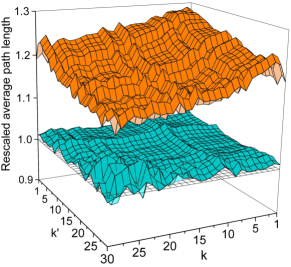
Figure 4: (Color online) Rescaled average shortest path length $\langle l(k,k^{\prime})\rangle_{\text{res}}$ between nodes of degree $k$ and $k^{\prime}$. The lower and upper surfaces represent the results for the Gnutella network and the coauthorship network, respectively. The bottom flat mesh indicates $\langle l(k,k^{\prime})\rangle_{\text{res}}=1$.

V Conclusions

In this paper, we have provided a general framework to analyze pairwise correlations between degrees of nodes at an arbitrary distance from each other in a complex network. In order to fully describe such long-range degree correlations (LRDCs) between degrees $k$ and $k^{\prime}$ of two nodes separated by $l$ in the sense of the shortest path length, we introduced the joint probability $P(k,k^{\prime},l)$ and four conditional probabilities $P(l|k,k^{\prime})$, $P(k^{\prime}|k,l)$, $P(k,k^{\prime}|l)$, and $P(k^{\prime},l|k)$. These probabilities are not independent, and several relations between them have been presented with the aid of the Bayes’ theorem. It has also been shown that the above probability functions include the probabilities $P_{\text{nn}}(k,k^{\prime})$ and $P_{\text{nn}}(k^{\prime}|k)$ describing nearest neighbor degree correlations as a special case. Furthermore, we have analytically calculated these five probabilities for a network without any degree correlations at an arbitrary distance under the local tree assumption and the mean-field approximation. The results for Erdős-Rényi random graphs and scale-free random networks agree well with numerical ones. The probabilities for long-range uncorrelated networks enable us to judge the existence of LRDCs in a given network and capture the feature of correlations. Finally, we analyzed LRDCs in real-world networks within the present framework and found that the coauthorship network possesses LRDCs in which small degree nodes strongly repel each other.

Although we have just prepared tools for analyzing LRDCs, it is quite interesting to study relations between LRDCs and many network properties such as the robustness of a network, fractality, synchronization, to name a few. Our joint and conditional probabilities are three-variable functions and are not easy to handle. Thus, it is also important to develop intuitive indices characterizing LRDCs, like a measure of the strength of the repulsive correlation between similar degree nodes, on the basis of these probabilities.

- (1) A.-L. Barabási and R. Albert, Science 286, 509 (1999).
- (2) R. Pastor-Satorras, A. Vázquez, and A. Vespignani, Phys. Rev. Lett. 87, 258701 (2001).
- (3) S. Maslov and K. Sneppen, Science 296, 910 (2002).
- (4) M. E. J. Newman, Phys. Rev. Lett. 89, 208701 (2002).
- (5) M. E. J. Newman, Phys. Rev. E 67, 026126 (2003).
- (6) J. Park and M. E. J. Newman, Phys. Rev. E 68, 026112 (2003).
- (7) M. Catanzaro, G. Caldarelli, and L. Pietronero, Phys. Rev. E 70, 037101 (2004).
- (8) M. A. Serrano, M. Boguñá, and R. Pastor-Satorras, Phys. Rev. E 74, 055101 (2006).
- (9) B. Fotouhi and M. G. Rabbat, Eur. Phys. J. B 86, 510 (2013).
- (10) N. Litvak and R. van der Hofstad, Phys. Rev. E 87, 022801 (2013).
- (11) S. N. Soffer and A. Vázquez, Phys. Rev. E 71, 057101 (2005).
- (12) M. A. Serrano and M. Boguñá, Phys. Rev. E 72, 036133 (2005).
- (13) J. C. Miller, Phys. Rev. E 80, 020901 (2009).
- (14) R. van der Hofstad, A. J. E. M. Janssen, J. S. H. van Leeuwaarden, and C. Stegehuis, Phys. Rev. E 95, 022307 (2017).
- (15) J. Menche, A. Valleriani, and R. Lipowsky, Phys. Rev. E 81, 046103 (2010).
- (16) R. Xulvi-Brunet and I. M. Sokolov, Phys. Rev. E 70, 066102 (2004)
- (17) S.-H. Yook, F. Radicchi, and H. Meyer-Ortmanns, Phys. Rev. E 72, 045105 (2005).
- (18) C. Song, S. Havlin, and H. A. Makse, Nat. Phys. 2, 275 (2006).
- (19) Z.-W. Wei and B.-H. Wang, Phys. Rev. E 94, 032309 (2016).
- (20) V. M. Eguíluz and K. Klemm, Phys. Rev. Lett. 89, 108701 (2002).
- (21) M. Boguñá and R. Pastor-Satorras, Phys. Rev. E 66, 047104 (2002).
- (22) M. Boguñá, R. Pastor-Satorras, and A. Vespignani, Phys. Rev. Lett. 90, 028701 (2003).
- (23) T. Gross, Carlos J. Dommar D’Lima, and B. Blasius, Phys. Rev. Lett. 96, 208701 (2006).
- (24) J. Hindes and I. B. Schwartz, Phys. Rev. E 95, 052317 (2017).
- (25) F. Sorrentino, M. di Bernardo, G. H. Cuéllar, and S. Boccaletti, Physica D 224, 123 (2006).
- (26) M. Di Bernardo, F. Garofalo, and F. Sorrentino, Int. J. Bifurcation Chaos 17, 3499 (2007).
- (27) M. D. LaMar and G. D. Smith, Phys. Rev. E 81, 046206 (2010).
- (28) C. E. La Rocca, L. A. Braunstein, and P. A. Macri, Physica A 390, 2840 (2011).
- (29) V. Avalos-Gaytan, J. A. Almendral, D. Papo, S. E. Schaeffer, and S. Boccaletti, Phys. Rev. E 86, 015101 (2012).
- (30) S. Jalan, A. Kumar, A. Zaikin, and J. Kurths, Phys. Rev. E 94, 062202 (2016).
- (31) Z. Rong, X. Li, and X. Wang, Phys. Rev. E 76, 027101 (2007).
- (32) Z. Rong and Z.-X. Wu, Europhys. Lett. 87, 30001 (2009).
- (33) S. Devlin and T. Treloar, Phys. Rev. E 80, 026105 (2009).
- (34) R. J. La, IEEE/ACM Trans. Netw. 25, 2484 (2017).
- (35) J. D. Noh, Phys. Rev. E 76, 026116 (2007).
- (36) A. V. Goltsev, S. N. Dorogovtsev, and J. F. F. Mendes, Phys. Rev. E 78, 051105 (2008).
- (37) C. M. Schneider, A. A. Moreira, J. S. Andrade Jr., S. Havlin, and H. J. Herrmann, Proc. Natl. Acad. Sci. 108, 3838 (2011).
- (38) T. Tanizawa, S. Havlin, and H. E. Stanley, Phys. Rev. E 85, 046109 (2012).
- (39) S. Watanabe and Y. Kabashima, Phys. Rev. E 94, 032308 (2016).
- (40) H. D. Rozenfeld, S. Havlin, and D. ben-Avraham, New J. Phys. 9, 175 (2007)
- (41) Y. Fujiki, S. Mizutaka, and K. Yakubo, Eur. Phys. J. B 90, 126 (2017).
- (42) C. Orsini, M. M. Dankulov, P. Colomer-de-Simón, A. Jamakovic, P. Mahadevan, A. Vahdat, K. E. Bassler, Z. Toroczkai, M. Boguñá, G. Caldarelli, S. Fortunato, and D. Krioukov, Nat. Commun. 6, 8627 (2015).
- (43) B. Tadić, S. Thurner, and G. J. Rodgers, Phys. Rev. E 69, 036102 (2004).
- (44) M. Boguñá, C. Castellano, and R. Pastor-Satorras, Phys. Rev. Lett. 111, 068701 (2013).
- (45) R. E. Boulos, A. Arneodo, P. Jensen, and B. Audit, Phys. Rev. Lett. 111, 118102 (2013).
- (46) L. W. Swanson, O. Sporns, and J. D. Hahn, Proc. Natl. Acad. Sci. 113, E5972 (2016).
- (47) D. Rybski, H. D. Rozenfeld, and J. P. Kropp, Euro. Phys. Lett. 90, 28002 (2010).
- (48) M. Mayo, A. Abdelzaher, and P. Ghosh, Comput. Soc. Netw. 2, 4 (2015).
- (49) A. Arcagni, R. Grassi, S. Stefani, and A. Torriero, Eur. J. Oper. Res. 262, 708 (2017).
- (50) A. Allen-Perkins, J. M. Pastor, and E. Estrada, Appl. Math. Comput. 311, 262 (2017).
- (51) More precisely, is the average degree of nodes separated by from all nodes of degree . In other words, is the average th neighbor degree of a typycal node of degree , where the typical node of degree is a node of degree with the average number of th neighbors.
- (52) S. Melnik and J. P. Gleeson, Preprint arXiv:1604.05521.
- (53) M. E. J. Newman, S. H. Strogatz, and D. J. Watts, Phys. Rev. E 64, 026118 (2001).
- (54) While Ref. Melnik16 calculates the distance distribution for a network consisting of a connected component, our treatment covers networks composed of multiple disconnected components.
- (55) http://snap.stanford.edu/data/p2p-Gnutella04.html
- (56) http://snap.stanford.edu/data/ca-CondMat.html
- (57) W.-Y. Zhang, Z.-W. Wei, B.-H. Wang, and X.-P. Han, Physica A 451, 440 (2016).