Rapid Bayesian Inference of Global Network Statistics Using Random Walks

Abstract

We propose a novel Bayesian methodology which uses random walks for rapid inference of statistical properties of undirected networks with weighted or unweighted edges. Our formalism yields high-accuracy estimates of the probability distribution of any network node-based property, and of the network size, after only a small fraction of network nodes has been explored. The Bayesian nature of our approach provides rigorous estimates of all parameter uncertainties. We demonstrate our framework on several standard examples, including random, scale-free, and small-world networks, and apply it to study epidemic spreading on a scale-free network. We also infer properties of the large-scale network formed by hyperlinks between Wikipedia pages.

Over the past few years, our lives have become increasingly dependent on large-scale networks. In addition to the original computer-based networks such as the World Wide Web and the Internet, many online social networks have emerged, notably Twitter and Facebook. Our professional and personal activities are influenced daily by knowledge-sharing online services such as Wikipedia and YouTube. More generally, complex networks describe a broad spectrum of systems in nature, science, technology, and society Albert2002 ; Newman2010 . Many of these networks are large and evolving, making investigation of their statistical properties a challenging task. In particular, estimating the network size becomes non-trivial if the network is too large to visit every node. Consequently, predicting various network statistics, typically from random samples of limited size, has attracted considerable attention in the literature Newman2003 ; Lee2006 ; Yoon2007 ; Estrada2010 ; Gjoka2010 ; Cooper2012 ; Bliss2014 ; zhang2015 .

Here we develop a Bayesian approach to network sampling by random walks (RWs) Yoon2007 ; Cooper2012 . Unlike previous results, our framework can be used to build posterior probability distributions for any network node-based quantity of interest. Our approach reproduces several previously known global network statistics estimators within a single formalism, automatically removes statistical biases caused by RW sampling Yoon2007 ; Estrada2010 , and yields standard results in the uniform sampling limit. Surprisingly, accurate estimates of various network properties, including its size, are obtained after examining only a small fraction of all network nodes.

Consider a RW on a network of $N$ nodes with weighted edges: $\{w_{ji}\}$, where $w_{ji}$ is the rate of transition from node $i$ to node $j$. At each step the walker will transition to a neighboring node with a probability $P(i\to j)=w_{ji}/\sum_{k\in\{nn\}_{i}}w_{ki}$, where the sum is over all nearest neighbors of node $i$. We subdivide all network nodes into sets $S_{x}$ based on the value of some property $x$, such as the number of links connected to the current node, known as the node degree Albert2002 ; there are $N_{x}$ nodes in each set and ${\cal N}_{x}$ distinct sets. We assume that the property in question is discrete; continuous properties can be discretized by binning. We focus on undirected networks with symmetric rates, $w_{ji}=w_{ij}$. In this case, the stationary probability for the RW to occupy node $i$, $\pi_{i}$, can be determined using the steady-state master equation vanKampen2007 ; Krapivsky2010 :

$$\sum_{j\in\{nn\}_{i}}[\pi_{j}P(j\to i)-\pi_{i}P(i\to j)]=0.$$ (1)

Equation (1) is satisfied if $\pi_{i}\sim w_{i}=\sum_{k\in\{nn\}_{i}}w_{ki}$, where $w_{i}$ is the total outward rate. For unweighted networks, the node’s stationary probability is proportional to its degree $k_{i}$ Noh2004 . With normalization, the stationary probabilities become $\pi_{i}=w_{i}/\sum_{i=1}^{N}w_{i}$.

If the walker starts from a node with property $x$, the average number of steps between subsequent visits to any node within the set $S_{x}$, also known as the mean return time (RT), is given by Condamin2007 :

$$\langle\ell\rangle_{x}=\frac{1}{\sum_{i\in S_{x}}\pi_{i}}.$$ (2)

In the case of undirected networks,

$$\langle\ell\rangle_{x}=\frac{\langle w\rangle}{p_{x}\langle w\rangle_{x}},$$ (3)

where $p_{x}=N_{x}/N$ is the fraction of nodes with property $x$, $\langle w\rangle=N^{-1}\sum_{i=1}^{N}w_{i}$, and $\langle w\rangle_{x}=N_{x}^{-1}\sum_{i=1}^{N_{x}}w_{i}$.

The probability of making $\Delta\ell$ steps between subsequent visits to $S_{x}$, $P(\Delta\ell)$, is asymptotically exponential in arbitrary finite networks Bollt2005 :

$$P(\Delta\ell)\simeq q_{x}e^{-q_{x}\Delta\ell}\;\text{ for }\;\Delta\ell=0,1,\dots,$$ (4)

where $q_{x}=\langle\ell\rangle_{x}^{-1}\ll 1$ is the hitting rate of the nodes within $S_{x}$. We find empirically that the exponential ansatz for $P(\Delta\ell)$ is sufficiently accurate for our purposes, although in principle our approach is not limited to it. The likelihood that during a single RW with $\ell\gg 1$ steps the walker has visited $\mathcal{K}_{x}$ nodes in $S_{x}$ is then given by the Poisson distribution:

$$P(\mathcal{K}_{x}|q_{x})=\frac{(q_{x}\ell)^{\mathcal{K}_{x}}}{\mathcal{K}_{x}!}e^{-q_{x}\ell}.$$ (5)

This likelihood function is maximized by $\hat{q}_{x}=\mathcal{K}_{x}/\ell$, which implies $\mathcal{K}_{x}\ll\ell$. Assuming a uniform prior for $q_{x}$ in the $[0,1]$ range, the posterior probability density for $q_{x}$ becomes

$$P(q_{x}|\mathcal{K}_{x})=\frac{1}{B(\mathcal{K}_{x},\ell)}q_{x}^{\mathcal{K}_{x}}e^{-q_{x}\ell},$$ (6)

where $B(\mathcal{K}_{x},\ell)=\int_{0}^{1}dq_{x}q_{x}^{\mathcal{K}_{x}}e^{-q_{x}\ell}\simeq\mathcal{K}_{x}!/\ell^{\mathcal{K}_{x}+1}$ is a normalization constant. Thus Eq. (6) is closely approximated by a gamma distribution $\Gamma(q_{x};\mathcal{K}_{x}+1,\ell)$, which becomes Gaussian in the $\mathcal{K}_{x}\gg 1$ limit, with the mean $\bar{q}_{x}=\hat{q}_{x}$ and the standard deviation $\sigma_{q_{x}}=\hat{q}_{x}/\sqrt{\mathcal{K}_{x}}$.

This result in combination with Eq. (3) yields a maximum likelihood estimate (MLE) and a standard error for the probability $p_{x}$ of the property $x$:

$$\hat{p}_{x}=\frac{\mathcal{K}_{x}/\langle w\rangle_{x}}{\sum_{x}^{{\cal N}_{x}}\mathcal{K}_{x}/\langle w\rangle_{x}}\;\text{ and }\;\sigma_{p_{x}}=\frac{\hat{p}_{x}}{\sqrt{\mathcal{K}_{x}}}.$$ (7)

If the property of the node $i$ is its total outward rate $w_{i}$ discretized into ${\cal N}_{w}$ bins, Eq. (7) yields

$$\hat{p}_{w_{i}}=\frac{\mathcal{K}_{w_{i}}/w_{i}}{\sum_{j=1}^{\mathcal{N}_{w}}\mathcal{K}_{w_{j}}/w_{j}},$$ (8)

where $\mathcal{K}_{w_{j}}$ is the number of visits to nodes with total outward rates in the bin $j$. For unweighted networks ($w_{ij}=1,\;\forall i,j$), $\hat{p}_{w_{i}}$ reduces to $\hat{p}_{k_{i}}$, the network degree distribution Albert2002 .

For an arbitrary node property $x$, each set $S_{x}$ can be additionally subdivided by the binned value of $w$, such that

$$\hat{p}_{x}=\sum_{j=1}^{{\cal N}_{w}}\hat{p}_{x,w_{j}}=\sum_{j=1}^{{\cal N}_{w}}\frac{\mathcal{K}_{x,w_{j}}}{w_{j}}/\sum_{j=1}^{{\cal N}_{w}}\frac{\mathcal{K}_{w_{j}}}{w_{j}}.$$ (9)

Here, $\mathcal{K}_{x,w_{j}}$ is the number of visits to nodes with both property $x$ and the total outward rates in the bin $j$. Thus, the knowledge of $\mathcal{K}_{w_{j}}$, $\mathcal{K}_{x,w_{j}}$, and $w_{j}$ is sufficient to compute the MLE of any property $x$ and estimate its uncertainty (Eq. (7)). Note that the division by $w_{j}$ in Eq. (9) corrects for the bias introduced by RW sampling Estrada2010 ; Yoon2007 ; Gjoka2010 .

The MLE of the average outward rate is given by

$$\hat{\langle w\rangle}=\sum_{i=1}^{\mathcal{N}_{w}}w_{i}\hat{p}_{w_{i}}=\frac{\ell}{\sum_{j=1}^{\mathcal{N}_{w}}\mathcal{K}_{w_{j}}/w_{j}},$$ (10)

where we used $\sum_{i=1}^{\mathcal{N}_{w}}\mathcal{K}_{w_{i}}=\ell$. The uncertainty of this estimate can be evaluated using $\sigma_{\langle w\rangle}^{2}=\sum_{i=1}^{\mathcal{N}_{w}}w_{i}^{2}\sigma^{2}_{p_{w_{i}}}$ as well as Eqs. (7) and (8), to yield $\sigma_{\langle w\rangle}=\hat{\langle w\rangle}/\sqrt{\ell}$, in accordance with the central limit theorem. Similarly, for an arbitrary property $x$

$$\hat{\langle x\rangle}=\sum_{x}x\hat{p}_{x}\;\text{ and }\;\sigma^{2}_{\langle x\rangle}=\sum_{x}x^{2}\sigma_{p_{x}}^{2}.$$ (11)

Let us now suppose that the network nodes are divided into two sets: $N_{p}$ randomly chosen nodes, which we shall refer to as pseudotargets, and all the rest. The pseudotarget nodes are drawn prior to exploring the network, so that their average outward rate, $\langle w\rangle_{p}$, is known. Equations (3) and (5) can now be used to construct the posterior probability for the network size (assuming a uniform prior in the $[N_{p},N_{max}]$ range, where $N_{max}$ denotes an upper limit on $N$):

$$P(N|\mathcal{K}_{p})=\frac{N^{-\mathcal{K}_{p}}\exp\left\{-\frac{N_{p}\langle w\rangle_{p}}{N\langle w\rangle}\ell\right\}}{\sum_{\tilde{N}=N_{p}}^{N_{max}}\tilde{N}^{-\mathcal{K}_{p}}\exp\left\{-\frac{N_{p}\langle w\rangle_{p}}{\tilde{N}\langle w\rangle}\ell\right\}},$$ (12)

where $\mathcal{K}_{p}$ is the number of visits to pseudotargets. Note that using uniform priors in both Eqs. (6) and (12) does not affect the results as long as $\mathcal{K}_{x}$ and $\mathcal{K}_{p}$, respectively, are sufficiently large. Similar to Eq. (6), we find that this posterior probability rapidly becomes Gaussian as $\mathcal{K}_{p}$ increases, with

$$\hat{N}=\frac{\ell N_{p}\langle w\rangle_{p}}{\mathcal{K}_{p}\langle w\rangle}\;\text{ and }\;\sigma_{N}=\frac{\hat{N}}{\sqrt{\mathcal{K}_{p}}}.$$ (13)

Using Eq. (10), we obtain

$$\hat{N}=\frac{N_{p}\langle w\rangle_{p}}{\mathcal{K}_{p}}\sum_{j=1}^{\mathcal{N}_{w}}\frac{\mathcal{K}_{w_{j}}}{w_{j}}.$$ (14)

Note that the error in $\hat{N}$ can be reduced either through increasing $N_{p}$ or assigning highly-connected nodes (network hubs) to be pseudotargets. In the $N_{p}=1$ case, Eq. (13) recovers the network size estimator from Ref. Cooper2012 .

Note that in the case of a complete unweighted network in which each node is connected to all $N$ nodes (including itself), RW sampling reduces to uniform sampling with replacement. In this limit, Eq. (7) yields $\hat{p}_{x}=\mathcal{K}_{x}/\ell$ and $\sigma_{p_{x}}=\sqrt{\mathcal{K}_{x}}/\ell$, consistent with the standard results based on binomial sampling. Moreover, $\hat{N}={\ell N_{p}}/{\mathcal{K}_{p}}$ in this case, reproducing the classic Lincoln-Petersen estimator of biological population sizes by the mark and recapture method Webster2013 (the differences between uniform sampling with and without replacement can be neglected in the $\mathcal{K}_{p}\ll N_{p}$ limit). These results remain valid for any network in which the total outward rate $w$ is the same for every node. Note that the key difference between RW sampling and uniform sampling is that the former preferentially visits the nodes with larger $w$ values, so that, given $\ell$, $\sigma_{p_{x}}$ is smaller for RW if $\langle w\rangle_{x}>\langle w\rangle$, and vice versa.

We have implemented the above theoretical framework as follows: for each network, $N_{p}$ pseudotargets are randomly drawn and their $\langle w\rangle_{p}$ is computed. Commencing the RW from one of these pseudotargets, we record $\ell$, $\mathcal{K}_{p}$, $\{\mathcal{K}_{w}\}$, and $\{\mathcal{K}_{x,w}\}$ for a desired set of node properties $x$. At each step in the RW, Eqs. (7)–(14) can then be used to infer various network properties.

Table 1: TDE model statistics summary. Shown are MLE and $95\%$ confidence interval ($\pm 2\sigma$) for each quantity, followed by exact values for the TDE model system. All predictions are based on a single representative RW with $\ell=10^{4}$ steps corresponding to the unit time interval in the TDE model.

$\hat{N}$	$N$	$\hat{\langle k\rangle}$	$\langle k\rangle$	$\savestack{\tmpbox}{\stretchto{\scaleto{\scalerel*[\widthof{\langle\langle k_{nn}\rangle\rangle}]{\kern 1.5pt\bigwedge\kern 1.5pt}{\rule[-505.89pt]{4.30554pt}{505.89pt}}}{}}{0.5ex}}\stackon[1.5pt]{\langle\langle k_{nn}\rangle\rangle}{\tmpbox}$	$\langle\langle k_{nn}\rangle\rangle$	$\hat{\langle C\rangle}$	$\langle C\rangle$	$\savestack{\tmpbox}{\stretchto{\scaleto{\scalerel*[\widthof{W/N}]{\kern 1.5pt\bigwedge\kern 1.5pt}{\rule[-505.89pt]{4.30554pt}{505.89pt}}}{}}{0.5ex}}\stackon[1.5pt]{W/N}{\tmpbox}$	$W/N$
$\pm 2\sigma_{N}$		$\pm 2\sigma_{\langle k\rangle}$		$\pm 2\sigma_{\langle\langle k_{nn}\rangle\rangle}$		$\pm 2\sigma_{\langle C\rangle}$		$\pm 2\sigma_{W/N}$
$1.01\times 10^{5}$	$10^{5}$	$8.02$	$8.14$	$64.6$	$67.1$	$0.251$	$0.255$	$2.000$	$2.000$
$\pm$ $0.08\times 10^{5}$		$\pm 0.16$		$\pm 4.2$		$\pm 0.011$		$\pm 0.045$

To verify the validity of our algorithm on standard model systems, we have studied three unweighted, undirected networks: an Erdős-Rényi (ER) random graph Erdos1961 , a scale-free (SF) random graph Albert2002 , and a small-world (SW) network Watts1998 . Each network has $N=10^{6}$ nodes. The ER network was constructed by randomly assigning $\lceil N\log(N)/2\rceil$ edges between nodes, the SF network by the preferential attachment method Albert2002 with $m=2$ edges attached to new nodes, and the SW network as described in Ref. Newman2000 , with the shortcut probability $p=1/2$.

For each network, $N_{p}=10^{3}$ pseudotargets were randomly drawn and the network was subsequently explored with a RW for $\ell=10^{5}$ steps, visiting at most 10% of all nodes. Besides network size and the node degree distribution, we have focused on posterior probabilities of the average degree of nearest-neighbor nodes, which is a measure of network degree assortativity,

$$\langle k_{nn}\rangle_{i}\equiv k_{i}^{-1}\sum_{j\in\{nn\}_{i}}{k_{j}},$$ (15)

the clustering coefficient Newman2003 ,

$$C_{i}\equiv\frac{2y}{k_{i}(k_{i}-1)},$$ (16)

where $y$ is the total number of links shared by the nearest neighbors of node $i$, and a measure of the degree inhomogeneity Estrada2010

$$\rho_{i}\equiv\sum_{j\in\{nn\}_{i}}\left(k_{i}^{-1/2}-k_{j}^{-1/2}\right)^{2}.$$ (17)

A comprehensive summary of the inferred network statistics can be found in the Supplementary Material (SM) SM2018 . Although network topologies of these three systems are quite different, all statistics we have considered are predicted accurately.

Next, we have constructed a generalized ER network with $N=10^{6}$ nodes and weighted edges. After placing all the edges as in the unweighted ER network, a loop was added to each node with probability $p=1/2$. All loops and edges were then assigned a symmetric weight $w_{ij}=w_{ji}$ drawn from an exponential distribution with unit mean. For this system, we have collected statistics on each node’s total outward rate, $w_{i}$, loop weight, $w^{\mathrm{loop}}_{i}=w_{ii}$ (note that $w_{ii}=0$ for nodes without loops), outward rate averaged over all nearest neighbors of node $i$, $\langle w_{nn}\rangle_{i}$, and average nearest-neighbor loop weight, $\langle w_{nn}^{\mathrm{loop}}\rangle_{i}$. We have again employed a RW with $\ell=10^{5}$ steps and $N_{p}=10^{3}$ randomly drawn pseudotargets. Although the RT distribution for this system deviates from purely exponential due to loops, all the network statistics we have considered are again predicted accurately SM2018 . Thus our methodology is equally applicable to studies of weighted networks with loops.

After validating our approach on model systems, we have demonstrated its effectiveness in a more realistic setting, by tracking an epidemic spreading on a scale-free network in the traffic-driven epidemiological (TDE) model Meloni2009 . Following Ref. Meloni2009 , we have generated the underlying network using a hidden-metric approach, which employs a tunable parameter $\alpha$ to control the degree of local node clustering Serrano2008 . The number of links in each node is drawn from a power-law distribution, $p_{k_{i}}\sim{k_{i}}^{-\gamma}$. For our network, we have chosen $N=10^{5}$, $\gamma=2.6$, and $\alpha=2$ (which leads to significant clustering).

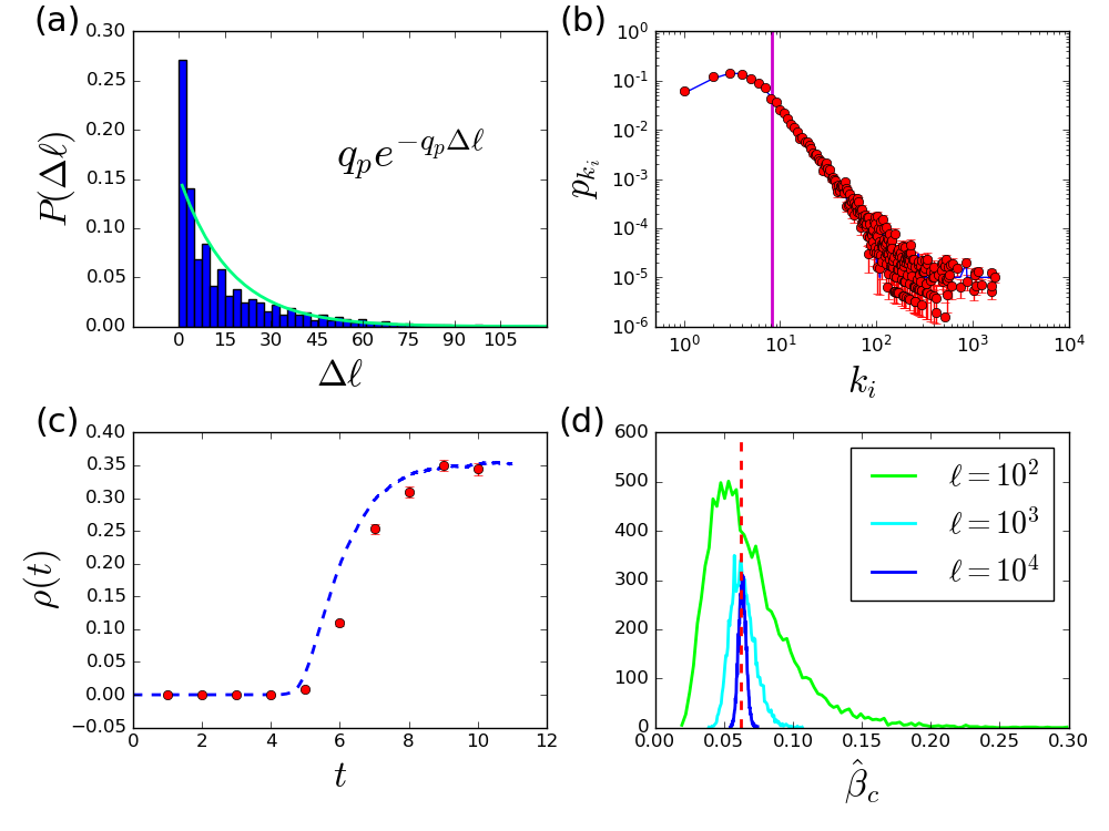
Figure 1: Epidemic spreading statistics. (a) Pseudotarget RT distribution. Equation (4) parameterized by exact $q_{p}$ is shown in cyan. (b) $\mathrm{MLE}\pm 2\sigma$ (red circles with error bars) for the node degree distribution; exact distribution is shown in blue and its average is shown as a vertical line. (c) $\mathrm{MLE}\pm 2\sigma$ (red circles with error bars) for the fraction of infected nodes $\rho(t)$ computed at unit time intervals, with the exact value shown as a dashed blue curve. (d) Histograms of $\beta_{c}$ MLEs obtained using $10^{4}$ independent runs with $\ell=10^{2}$, $10^{3}$, $10^{4}$ steps. Exact value is shown as a vertical dashed line.

Epidemic propagation was simulated through the exchange of $W$ contagion packets between nodes (see Ref.  Meloni2009 for details). Briefly, each node can be in either susceptible or infected state; the simulation starts with a single infected node. When a packet moves from node $i$ to node $j$ on the network, node $j$ becomes infected with the spreading probability $\beta$ if node $i$ was infected; infected nodes can also recover with rate $\mu$, set to $1$ without loss of generality. We have focused on the case in which contagion packets perform RWs between randomly assigned initial and destination nodes. Once a packet reaches its destination, it is removed and a new packet is added to keep $W$ constant. On average, each packet moves once per unit simulation time. Under this choice of packet dynamics, there is a critical value of $\beta_{c}=(\langle k\rangle^{2}/\langle k^{2}\rangle)N/W$ above which a sustained epidemic outbreak is observed Meloni2009 . We have set $W=2N$ and $\beta=7\times 10^{-1}\gg\beta_{c}=6.24\times 10^{-2}$ in the simulation.

We have used a single RW with $\ell=10^{4}$ steps and $N_{p}=10^{3}$ pseudotargets to verify the validity of our exponential ansatz (Fig. 1(a)) and predict the node degree distribution (Fig. 1(b)); several other statistics relevant to the study of epidemics on networks Pellis2015 are listed in Table 1. In addition, we have tracked time-dependent evolution of the fraction of infected nodes $\rho(t)$ (Fig. 1(c)). We have assumed that nodes can be queried much faster than the time scales on which the epidemic spreads, and thus matched $\ell$ steps of our RW sampling to the unit time interval in the TDE model (Fig. 1(c), Table 1). Finally, we have predicted $\beta_{c}$ using the evolving system’s snapshot, again under the assumption that RW sampling is fast compared to the time scales of the epidemics (Fig. 1(d)).

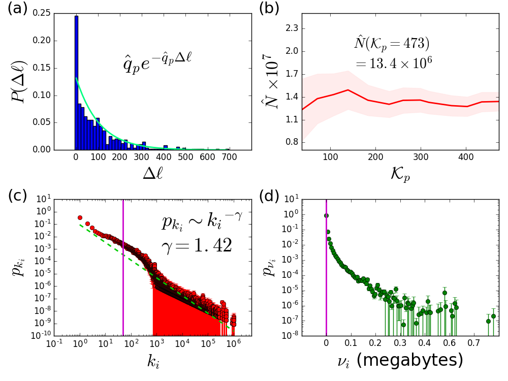
Figure 2: Wikipedia network statistics. (a) Pseudotarget RT distribution. Equation (4) parameterized by $\hat{q}_{p}$ is shown in cyan. (b) $\mathrm{MLE}\pm 2\sigma$ for $N$ as a function of ${\cal K}_{p}$. (c) $\mathrm{MLE}\pm 2\sigma$ for the degree distribution of Wikipedia pages of all types. Power-law fit is shown as a green dashed line. Average degree is shown as a vertical line. (d) $\mathrm{MLE}\pm 2\sigma$ for the distribution of Wikipedia page sizes. Average size is shown as a vertical line.

Table 2: Wikipedia statistics summary. Shown are MLE$\pm 2\sigma$ for each quantity. All predictions are based on a single trial with $\ell=5\times 10^{4}$ steps. $N_{a}$ and $N_{r}$ are the total number of English articles and redirect pages in Wikipedia, as of Dec. 2017 WikiPage2 .

$\hat{N}$	$\hat{\langle k\rangle}$	$\savestack{\tmpbox}{\stretchto{\scaleto{\scalerel*[\widthof{\langle\chi_{r}\rangle}]{\kern 1.5pt\bigwedge\kern 1.5pt}{\rule[-505.89pt]{4.30554pt}{505.89pt}}}{}}{0.5ex}}\stackon[1.5pt]{\langle\chi_{r}\rangle}{\tmpbox}$	$\savestack{\tmpbox}{\stretchto{\scaleto{\scalerel*[\widthof{\langle\chi_{d}\rangle}]{\kern 1.5pt\bigwedge\kern 1.5pt}{\rule[-505.89pt]{4.30554pt}{505.89pt}}}{}}{0.5ex}}\stackon[1.5pt]{\langle\chi_{d}\rangle}{\tmpbox}$	$\savestack{\tmpbox}{\stretchto{\scaleto{\scalerel*[\widthof{\langle\nu_{a}\rangle}]{\kern 1.5pt\bigwedge\kern 1.5pt}{\rule[-505.89pt]{4.30554pt}{505.89pt}}}{}}{0.5ex}}\stackon[1.5pt]{\langle\nu_{a}\rangle}{\tmpbox}$	$\hat{\langle\nu\rangle}$	$\hat{N}(1-\savestack{\tmpbox}{\stretchto{\scaleto{\scalerel*[\widthof{\langle\chi_{r}\rangle}]{\kern 1.5pt\bigwedge\kern 1.5pt}{\rule[-505.89pt]{4.30554pt}{505.89pt}}}{}}{0.5ex}}\stackon[1.5pt]{\langle\chi_{r}\rangle}{\tmpbox})$	$N_{a}$	$\hat{N}\savestack{\tmpbox}{\stretchto{\scaleto{\scalerel*[\widthof{\langle\chi_{r}\rangle}]{\kern 1.5pt\bigwedge\kern 1.5pt}{\rule[-505.89pt]{4.30554pt}{505.89pt}}}{}}{0.5ex}}\stackon[1.5pt]{\langle\chi_{r}\rangle}{\tmpbox}$	$N_{r}$	$\hat{N}\savestack{\tmpbox}{\stretchto{\scaleto{\scalerel*[\widthof{\langle\nu_{a}\rangle}]{\kern 1.5pt\bigwedge\kern 1.5pt}{\rule[-505.89pt]{4.30554pt}{505.89pt}}}{}}{0.5ex}}\stackon[1.5pt]{\langle\nu_{a}\rangle}{\tmpbox}$
$\pm 2\sigma_{N}$	$\pm 2\sigma_{\langle k\rangle}$	$\pm 2\sigma_{\langle\chi_{r}\rangle}$	$\pm 2\sigma_{\langle\chi_{d}\rangle}$	$\pm 2\sigma_{\langle\nu_{a}\rangle}$	$\pm 2\sigma_{\langle\nu\rangle}$	$\pm 2\sigma_{N(1-\langle\chi_{r}\rangle)}$		$\pm 2\sigma_{N\langle\chi_{r}\rangle}$		$\pm 2\sigma_{N\langle\nu_{a}\rangle}$
$13.4\times 10^{6}$	$47.7$	$0.6009$	$0.0399$	$2670$	$2720$	$5.35\times 10^{6}$	$5.3\times 10^{6}$	$8.05\times 10^{6}$	$8.0\times 10^{6}$	$35.8$
$\pm 1.2\times 10^{6}$	$\pm 0.4$	$\pm 0.0197$	$\pm 0.0047$	$\pm 40\text{ bytes}$	$\pm 40\text{ bytes}$	$\pm 0.56\times 10^{6}$		$\pm 0.79\times 10^{6}$		$\pm 3.3\text{ GB}$

Next, we have examined the network formed by hyperlinks between English articles on Wikipedia. Links connecting an article to itself were disregarded, multiple links between articles were counted as one, and automatic redirects were disallowed, resulting in an unweighted, undirected, loopless network consisting of all English articles, redirect pages, and disambiguation pages WikiPage . To assign pseudotargets, the first $5000$ pages were drawn from Wikipedia’s static HTML dumps. A single randomly chosen link was then taken from each of these pages and the node it pointed to was designated as a pseudotarget, resulting in $N_{p}=4769$. This procedure increases the likelihood that the pseudotargets are hubs with a large number of links, facilitating collection of the network statistics since $\mathcal{K}_{p}$ grows more rapidly Noh2004 ; Lee2006 ; Cooper2012 .

We have focused on several statistics that facilitate comparison with known properties of Wikipedia: the size of each page in bytes, $\nu$ (as provided by Wikipedia), and two variables $\chi_{r},\chi_{d}\in\{0,1\}$ representing whether a page is a redirect or a disambiguation page, respectively. The quantities $\langle\chi_{r}\rangle$, $\langle\chi_{d}\rangle$, and $\langle\nu_{a}\rangle\equiv\langle(1-\chi_{r})\nu\rangle$ then give the fraction of redirect pages, disambiguation pages, and the average storage space in bytes of English articles (Wikipedia excludes redirect pages from its estimates of the number of articles WikiPage ). The RW was run for $\ell=5\times 10^{4}$ steps, with the resulting predictions shown in Table 2 and Fig. 2.

We find that Wikipedia contains $13.4$ million pages, each of which is connected on average to $48$ other pages. The majority of Wikipedia pages, $60\%$, are redirect pages, and $4\%$ are disambiguation pages. We estimate the total number of English articles (including disambiguation pages) to be $5.35$ million, and the total number of redirect pages to be $8.05$ million, within the confidence intervals of the values reported by Wikipedia WikiPage2 (Table 2). We find the total size of English articles in Wikipedia to be $35.8$ gigabytes (GB), in reasonable agreement with the Wikipedia statement that text alone accounts for $27.6$ GB of the storage space of English articles WikiPage3 .

Fig. 2(a) demonstrates that the assumption of the exponential RT distribution is reasonable for Wikipedia, with some enrichment for short RTs due to the choice of network hubs as pseudotargets. Fig. 2(b) shows how the estimate of the total number of Wikipedia pages evolves as ${\cal K}_{p}$ increases. As in many other Internet-based networks Faloutsos1999 , the degree distribution of Wikipedia pages is scale-free (Fig. 2(c)). In contrast, the distribution of page sizes is not scale-free, and the size of an average Wikipedia page is only $2.7$ kB (Fig. 2(d), Table 2).

In conclusion, we have presented a general Bayesian approach to inferring various network properties, including its size, by using RWs that visit only a small fraction of all network nodes. Our approach works for both weighted and unweighted undirected networks, and remains accurate in the presence of loops. Our main assumption, that of the exponentiality of the RT distribution, appears to hold in all the cases we have examined explicitly, and can be relaxed if necessary. Our future work will focus on extending this methodology to directed and time-dependent networks.

References

- (1) R. Albert and A. L. Barabási. Statistical mechanics of complex networks. Rev Mod Phys, 74:47–97, 2002.
- (2) M. E. J. Newman. Networks: An Introduction. Oxford University Press, 2010.
- (3) M. E. J. Newman. Mixing patterns in networks. Phys Rev E, 67:026126, 2003.
- (4) S. H. Lee, P.-J. Kim, and J. Hawoong. Statistical properties of sampled networks. Phys Rev E, 73:016102, 2006.
- (5) S. Yoon, S. Lee, S.-H. Yook, and Y. Kim. Statistical properties of sampled networks by random walks. Phys Rev E, 75:046114, 2007.
- (6) E. Estrada. Quantifying network heterogeneity. Phys Rev E, 82:066102, 2010.
- (7) M. Gjoka, M. Kurant, C. T. Butts, and A. Markopoulou. Walking in Facebook: A case study of unbiased sampling of OSNs. In Proc 29th Conf Inform Comm, INFOCOM’10, pages 2498–2506, Piscataway, NJ, USA, 2010. IEEE Press.
- (8) C. Cooper, T. Radzik, and Y. Siantos. Estimating network parameters using random walks. In 2012 Fourth International Conference on Computational Aspects of Social Networks (CASoN), pages 33–40, Nov 2012.
- (9) C. A. Bliss, C. M. Danforth, and P. S. Dodds. Estimation of global network statistics from incomplete data. PLoS One, 9:e108471, 2014.
- (10) Y. Zhang, E. D. Kolaczyk, and B. D. Spencer. Estimating network degree distributions under sampling: An inverse problem, with applications to monitoring social media networks. Ann Appl Stat, 9:166–199, 2015.
- (11) N. G. van Kampen. Stochastic Processes in Physics and Chemistry. Elsevier, Amsterdam, 2007.
- (12) P. L. Krapivsky, S. Redner, and E. Ben-Naim. A Kinetic View of Statistical Physics. Cambridge University Press, 2010.
- (13) J. D. Noh and H. Rieger. Random walks on complex networks. Phys Rev Lett, 92:118701, 2004.
- (14) S. Condamin, O. Benichou, and M. Moreau. Random walks and Brownian motion: a method of computation for first-passage times and related quantities in confined geometries. Phys Rev E, 75:021111, 2007.
- (15) E. M. Bollt and D. ben-Avraham. What is special about diffusion on scale-free nets? New J Phys, 7:26–47, 2005.
- (16) A. J. Webster and R. Kemp. Estimating omissions from searches. Amer. Stat., 67:82–89, 2013.
- (17) P. Erdos and A. Renyi. On the evolution of random graphs. Bull Inst Internat Stat, 38:343–347, 1961.
- (18) D. J. Watts and S. H. Strogatz. Collective dynamics of small-world networks. Nature, 393:440–442, 1998.
- (19) M. E. J. Newman, C. Moore, and D. Watts. Mean-field solution of the small-world network model. Phys Rev Lett, 84:3201–3204, 2000.
- (20) See Supplemental Material at [URL will be inserted by publisher] for additional network inference results.
- (21) S. Meloni, A. Arenas, and Y. Moreno. Traffic-driven epidemic spreading in finite-size scale-free networks. Proc Nat Acad Sci USA, 106:16897–16902, 2009.
- (22) M. A. Serrano, D. Krioukov, and M. Boguna. Self-similarity of complex networks and hidden metric spaces. Phys Rev Lett, 100:078701, 2008.
- (23) L. Pellis, F. Ball, S. Bansal, K. Eames, T. House, V. Isham, and P. Trapman. Eight challenges for network epidemic models. Epidemics, 10:58–62, 2015.
- (24) https://en.wikipedia.org/wiki/Wikipedia:What_is_an_article?
- (25) https://stats.wikimedia.org/EN/TablesWikipediaEN.htm.
- (26) https://en.wikipedia.org/wiki/Wikipedia:Size_in_volumes.
- (27) M. Faloutsos, P. Faloutsos, and C. Faloutsos. On power-law relationships of the internet topology. SIGCOMM Comput Commun Rev, 29:251–262, 1999.