Sparse principal component analysis and its $\ell_{1}$-relaxation

Abstract

Principal component analysis (PCA) is one of the most widely used dimensionality reduction methods in scientific data analysis. In many applications, for additional interpretability, it is desirable for the factor loadings to be sparse, that is, we solve PCA with an additional cardinality ($\ell_{0}$-norm) constraint. The resulting optimization problem is called the sparse principal component analysis (SPCA). One popular approach to achieve sparsity is to replace the $\ell_{0}$-norm constraint by an $\ell_{1}$-norm constraint. In this paper, we prove that, independent of the data, the optimal objective function value of the problem with $\ell_{0}$ constraint is within a constant factor of the the optimal objective function value of the problem with $\ell_{1}$ constraint. To the best of our knowledge, this is the first formal relationship established between the $\ell_{0}$ and the $\ell_{1}$ constraint version of the problem.
Keywords. $\ell_{1}$ regularization, Sparsity, Principal component analysis

1 Introduction

Principal component analysis (PCA).

PCA [17] is one of the most widely used dimensionality reduction methods pervasive in statistics, data science and scientific data analysis [20]. Given a data matrix ${Y}_{m\times n}$ (with $m$ samples and $n$ features; and each feature is centered to have zero mean), the task of PCA is to find a direction ${x}\in\mathbb{R}^{n}$ (with $\|{x}\|_{2}=1$) such that it maximizes the variance of a weighted combination of the features, given by: ${Y}{v}$. If $A:=\frac{1}{m}Y^{\top}Y$ denotes the sample covariance matrix of ${Y}$, then a principal component (PC) direction can be found by

$$\textup{max}_{x}~{}~{}~{}{x}^{\top}A{x}~{}~{}\text{s.t.}~{}~{}\|{x}\|_{2}=1.$$ (1)

A maximizer $\hat{{x}}$ of (1) can be computed in polynomial time via a rank one eigendecompostion [12] of $A$. The entries of $\hat{x}$ are known as the factor loadings, and they lead to the first principal component direction ${Y}{\hat{x}}$, a linear combination of the features with maximal variance. PCA is widely used in microarray analysis [14, 26], handwritten zip code classification [15], human face recognition [13], image processing [18], text processing [31], financial analysis [28, 34] among others [27].

Sparse PCA.

An obvious drawback of PCA is that all the entries of $\hat{{x}}$ are nonzero, which leads to the PC direction being a linear combination of all features – this impedes interpretability [5, 21, 36]. In microarray analysis for example, when ${Y}$ corresponds to the gene-expression measurements for different samples, it is desirable to obtain a PC direction which involves only a handful of the features (i.e., genes) for interpretation purposes. In financial applications (where, $A$ denotes the sample covariance matrix of stock-returns), a sparse subset of stocks that are responsible for driving the first PC direction may be desirable for interpretation purposes. Thus in many scientific and industrial applications, for additional interpretability, it is desirable for the factor loadings to be sparse, i.e., few of the entries in $\hat{x}$ are nonzero and the rest are zero. This motivates the notion of a sparse principal component analysis (SPCA) [21, 16], wherein, in addition to maximizing the variance, one also desires the direction of the first PC to be sparse in the factor loadings. The most natural optimization formulation of this problem, modifies criterion (1) with an additional sparsity constraint on $x$ leading to:

$$\textup{max}_{x}~{}~{}~{}{x}^{\top}A{x}~{}~{}\text{s.t.}~{}~{}\|{x}\|_{2}=1,\|x\|_{0}\leq k,$$ (2)

where, $\|x\|_{0}\leq k$ allows at most $k$ of the entries in $x$ to be nonzero.

In addition to interpretability, sparsity is a key dimensionality reduction tool needed for meaningful statistical inference. For example, suppose $Y$ is a data matrix that is generated from a spiked covariance model with $\Sigma=\tau\theta\theta^{\top}+\sigma^{2}\mathbb{I}$ where, $\theta\in\mathbb{R}^{n}$ with $\|\theta\|_{2}=1$ and $\mathbb{I}$ denotes the identity matrix. Under the classical asymptotic regime, i.e., as the number of samples $m\rightarrow\infty$ with $n$ fixed, the first PC direction or the eigenvector of the sample covariance matrix $A$ is consistent [1] (up to sign changes) for the population version $\theta$. However, when $m,n$ are comparable with $\tfrac{m}{n}\rightarrow c\in(0,\infty)$ as $m\rightarrow\infty$ this classical consistency theory breaks down. The sample PC may no longer be consistent for the population version $\theta$, if $\tau/\sigma^{2}$ is sufficiently small – see [19] for additional details. In such situations, additional structure such as sparsity assumptions on $\theta$ are called for.

The SPCA problem has received significant attention in the wider statistics community since 1990s [5]; and influential follow-up work by [21, 36, 29, 33, 19], among many others. [22, 24] study well-grounded nonlinear optimization algorithms based on modifications of the power method for SPCA-type problems.

Enforcing $\ell_{1}$ constraint in place of $\ell_{0}$ constraint.

Unlike usual PCA, the sparse variant, Problem (2) is no longer easy to compute—several approaches and computational schemes have been proposed to address this problem. One of the most popular approaches is to relax the cardinality constraint $\|v\|_{0}\leq k$ by an $\ell_{1}$ aka Lasso [30] constraint, leading to

$$\textup{max}_{x}~{}~{}~{}{x}^{\top}A{x}~{}~{}\text{s.t.}~{}~{}\|{x}\|_{2}=1,\|x\|_{1}\leq\delta,$$ (3)

for some $\delta>0$. Criterion (3) was proposed in [21]. Criterion (3) is appealing as it uses a soft version of sparsity akin to Lasso regression: the $\ell_{1}$-constraint on $x$ induces both sparsity and shrinkage in a continuous fashion via the tuning parameter $\delta$; unlike Problem (2) which produces a discrete set of solutions for every $k\in[n]$. In addition, the $\ell_{1}$-constraint may be suitable when some entries of $x$ are small (instead of being exactly zero) and the others are large. The papers [32, 2] have studied minimax optimal properties of the estimator (3) under a spiked covariance model, under the assumption that the population eigenvector lies in the $\ell_{1}$ ball.

Problem (3) is a continuous optimization problem unlike Problem (2) and hence more amenable to techniques in nonlinear continuous optimization: [21] propose to use a projected gradient method for Problem (3). Note however that unlike the Lasso version of best-subset selection which is convex; Problem (3) is a difficult nonconvex optimization task; and computing optimal solutions may be difficult. [33] (see also Chapter 8 [16]) argue that developing an iterative scheme towards optimization of (3) is not straightforward and hence consider a close cousin given by:

$$\textup{max}_{x,y}~{}~{}~{}{y}^{\top}Y{x}~{}~{}\text{s.t.}~{}~{}\|{y}\|_{2}=1,\|x\|_{1}\leq\delta,\|x\|_{2}=1,$$ (4)

where, $Y$ is the data-matrix (recall that $A=\tfrac{1}{m}Y^{\top}Y$). [33, 16] propose a clever alternating optimization scheme for Problem (4).

Our result: formal relation between enforcing $\ell_{1}$ constraint and the $\ell_{0}$ constraint.

Unlike the literature on sparse regression, the literature on SPCA treats the $\ell_{0}$ and $\ell_{1}$ constraints separately, for example, deriving separate semi-definite programming (SDP) relaxations [8, 34]. To the best of our knowledge, there is no theoretical results comparing the solutions or the optimal objective function value of the problems with $\ell_{0}$ and $\ell_{1}$ constraints.

In the context of SPCA, note that the constraints $\|x\|_{0}\leq k$ and $\|x\|_{2}\leq 1$ together imply that $\|x\|_{1}\leq\sqrt{k}$. Thus, for $\delta=\sqrt{k}$, (3) is relaxation of (2). It therefore makes sense to compare (2) and (3) with $\delta=\sqrt{k}$. Henceforth we refer to (3) with $\delta=\sqrt{k}$ as the $\ell_{1}$-relaxation of SPCA.

In this paper we prove that, independent of $A$, the optimal objective function of SPCA (i.e, (2)) is within a constant factor of the optimal objective function of the $\ell_{1}$-relaxation of SPCA (i.e. (3) with $\delta=\sqrt{k}$). Our proof of this result is via a randomized rounding argument, thus yielding a constant factor approximation algorithm to solve SPCA assuming we have access to the optimal solution of its $\ell_{1}$-relaxation. Moreover, our result holds more generally when ${x}^{\top}A{x}$ in the objective is replaced by any semi-norm. Therefore, instead of maximizing $\|Yx\|^{2}_{2}$ (which is the same as maximizing ${x}^{\top}A{x}$), if we maximize $\|Yx\|_{1}$ in (2) and (3) with $\delta=\sqrt{k}$, the constant factor result still holds. We note that such $\ell_{1}$-norm objectives in the context of PCA has been studied [25].

It is intriguing to compare our result on the role played by $\ell_{1}$-constraint in the context of PCA to the same in the context of best-subsets selection. The pioneering work by Donoho [9], Candes and Tao [7], and Candes et al. [6], showed that sparse solutions to under-determined system of equations may be retrieved by replacing the $\ell_{0}$-pseudo norm by a $\ell_{1}$ norm. However this result holds only under the assumption that the data matrix satisfies certain conditions such as the “restricted isometry property”. The noisy version of the problem requires additional assumptions on the problem data, and for support recovery additional assumptions (such as the irrepresentable condition) are needed–see for e.g., [35, 4]. Our result on the constant factor approximation; on the other hand, does not require any assumption on $A$ – and holds universally – making it quite different from the existing results for $\ell_{0}$-$\ell_{1}$-equivalence in the context of sparse regression. We do note however, that the $\ell_{1}$-version of the problem for sparse linear regression is a convex optimization problem; and hence computable in polynomial time – both the problems (2) and (3) are NP-hard.

We finally note here that the paper [11] presented for the first time the simple randomized algorithm used for our analysis. This algorithm starts with a solution of $\ell_{1}$-relaxation of SPCA (i.e. (3) with $\delta=\sqrt{k}$) and randomly rounds it to produce sparsity. Loosely speaking, the result obtained in [11] is of the following form: While with high probability the additive difference in the objective function value of $\ell_{1}$-relaxation and the objective function value of the randomly obtained vector is bounded by $\epsilon$, the expected sparsity of the randomly obtained vector is $\frac{200k}{\epsilon}$ which is significantly larger than $k$. Therefore, this result does not establish a relationship between SPCA and the $\ell_{1}$-relaxation for the same value of $k$. Our analysis explicitly accounts for the positive semi-definiteness of $A$, which is not used in the analysis presented in [11].

2 Main results

For an integer $t\geq 1$, we use $[t]$ to describe the set $\{1,\dots,t\}$. Also, we represent the $j^{\text{th}}$ unit vector, the vector of ones, and the vector of zeros in appropriate dimension by $e_{j}$, $\boldsymbol{1}$, and $\boldsymbol{0}$, respectively.

Since the square root function is monotonic, note that the objective function in (2) and (3) can be replaced by $\sqrt{{x}^{\top}A{x}}$ and the resulting problem has the same set of optimal solutions. We denote $\sqrt{{x}^{\top}A{x}}$ by $\|x\|_{A}$.

As mentioned in the previous section, our main result holds for more general objective functions than that of $\|x\|_{A}$. Let $\phi:\mathbb{R}^{n}\rightarrow\mathbb{R}_{+}$ be a semi-norm, i.e., (i) $\phi$ is positively-homogenous: $\phi(\lambda x)=\lambda\phi(x)$ for all $\lambda\geq 0$, (ii) $\phi$ is subadditive: $\phi(u+v)\leq\phi(u)+\phi(v)$ for all $u,v\in\mathbb{R}^{n}$, (iii) $\phi$ is nonnegative: $\phi(u)\geq 0$ for all $u\in\mathbb{R}^{n}$, and (iv) $\phi(\textbf{0})=0$. Conditions (i) and (ii), imply that $\phi$ is a convex function. Also note that $\phi(x)=0$ does not imply that $x=\textbf{0}$.

Since $A$ is positive semi-definite, it is straightforward to verify that $\|x\|_{A}$ is semi-norm. We now present the general version of sparse PCA, which we call as the semi-norm SPCA, and its $\ell_{1}$-relaxation, corresponding to an arbitrary semi-norm $\phi$:

$$\begin{array}[]{rc}\textsc{OPT}_{\ell_{0}}\triangleq\textup{max}_{x}&\phi(x)\\ \textup{s.t.}&\|x\|_{2}\leq 1\\ &\|x\|_{0}\leq k,\end{array}$$ (Semi-norm SPCA)

$$\begin{array}[]{rcl}\textsc{OPT}_{\ell_{1}}\triangleq\textup{max}_{x}&\phi(x)&\\ \textup{s.t.}&\|x\|_{2}&\leq 1\\ &\|x\|_{1}&\leq\sqrt{k}.\end{array} \ell_{1}$$ (-norm relaxation)

In order to convert a solution for the $\ell_{1}$-norm relaxation to a solution for Semi-norm SPCA, we consider the simple randomized rounding procedure of [11]:

Algorithm 1 Randomized rounding of solution of $\ell_{1}$-relaxation

1:Input: the optimal solution $x$ to the $\ell_{1}$-norm relaxation, and parameters $\gamma\in(0,1)$, $g\in\mathbb{R}_{+}$

2:Let $p_{i}=\min\{s\frac{|x_{i}|}{\|x\|_{1}},1\}$, where $s=\gamma\cdot k$

3:Let $\varepsilon_{i}\in\{0,1\}$ take the value 1 with probability $p_{i}$, and the value 0 with probability $1-p_{i}$

4:Let the $i$-th coordinate of the randomly rounded solution be:

$$X_{i}=\frac{1}{p_{i}}\,x_{i}\varepsilon_{i}$$

5:Output the solution $\frac{X}{g}$

Our main result is an analysis of this procedure that shows that the $\ell_{1}$-norm relaxation is within a constant factor of the Semi-norm SPCA.

Theorem 1.

For any semi-norm $\phi:\mathbb{R}^{n}\rightarrow\mathbb{R}_{+}$ and $k\geq 15$, we have that

$$\textsc{OPT}_{\ell_{0}}\leq\textsc{OPT}_{\ell_{1}}\leq 2.95\cdot\textsc{OPT}_{\ell_{0}}.$$

Moreover, with positive probability, the solution $\frac{X}{g}$ output by Algorithm 1 with $\gamma=0.4051$ and $g=2.996$ is feasible for the Semi-norm SPCA problem and satisfies: $\phi(\frac{X}{g})\geq\frac{1}{3.25}\,\textsc{OPT}_{\ell_{1}}$.

We note that the constants $2.95$ and $3.25$ can be improved if one considers higher values of the lower bound on $k$. Also with a small additional loss to the constant $3.25$, the success probability of the algorithm can be boosted to an arbitrary constant (by also running the rounding procedure multiple times).

The high-level idea of the proof is the following: We need to show that with positive probability, $\frac{X}{g}$ is feasible for the Semi-norm SPCA and has large objective value. Standard concentration shows that feasibility holds with “large” constant probability. To control the value, notice that the rounding in unbiased, namely $\mathbb{E}X=x$, and that $\phi$ is convex. Thus, the expected objective value of our unscaled solution is large: $\mathbb{E}\phi(X)\geq\phi(\mathbb{E}X)=\phi(x)=\textsc{OPT}_{\ell_{0}}$ (the scaling only introduces an additional $\frac{1}{g}$ factor in the bound).

The issue is that, in principle, our solution $X$ could take a very objective large value with very small probability (and this happening when it is infeasible), and taking very small value with probability close to 1. To show that this does not happen, we need to control the upper tail of $\phi(X)$ (and with something more effective than Markov’s inequality).

However, it is not clear how to obtain concentration for $\phi(X)$ since we cannot control its “Lipschitzness”; for example, in the special case $\phi=\|.\|_{A}$, we do not have any assumptions on the magnitude of the entries of $A$, and in particular its relationship to $\textsc{OPT}_{\ell_{0}}$.

To handle this issue, we use solely $\|X\|_{0}$ and $\|X\|_{2}$ to control $\phi(X)$. More specifically, we upper bound the largest possible objective value of a solution with $\|.\|_{0}=t$ and $\|.\|_{2}=w$, and show that it is at most $\approx w\sqrt{t/k}\,\textsc{OPT}_{\ell_{0}}$ (Lemma 5); this provides and upper bound on $\phi(X)$ as long as $\|X\|_{0}\leq t$ and $\|X\|_{2}\leq w$. Then, the we obtain the desired control over the behavior of $\phi(X)$ by employing concentration for $\|.\|_{0}$ and $\|.\|_{2}$ and carefully integrating over $t$ and $w$.

A natural question is how good the constant $2.95$ presented in Theorem 1 is; we present a lower bound on this constant.

Theorem 2.

There exists a rank one positive-semidefinite matrix $A$ such that with $\phi=\|.\|_{A}$ we have that

$$\textsc{OPT}_{\ell_{1}}\geq 1.32\cdot\textsc{OPT}_{\ell_{0}}.$$

Since there is a big gap between the upper and lower bounds obtained on the worst-case value of the multiplicative constant factor, it is an open question which of them is closer to the actual worst-case bound. In our limited computational experiments, we saw ratios significantly lesser than $1.32$, so we speculate that the lower bound of $1.32$ is perhaps closer to the actual constant.

3 Proof of Theorem 1

3.1 Preliminaries

In this section we collect a few technical results that will be needed in the sequel. The first is a simple observation on the arithmetico-geometric series, for which we include a proof for completeness.

Lemma 1.

$\sum_{t=k}^{n}te^{-t}\leq\eta(k)\triangleq e^{-k}\left[\frac{ke^{2}-(k-1)e}{(e-1)^{2}}\right]$.

Proof.

Let $S:=\sum_{t=k}^{n}te^{-t}$. Then $eS=\sum_{t=k}^{n}te^{-(t-1)}$ and therefore

$$(e-1)S=ke^{-k+1}+\sum_{t=k+1}^{n}e^{-(t-1)}-ne^{-n}\leq ke^{-k+1}+\sum_{t=k+1}^{\infty}e^{-(t-1)}\leq ke^{-k+1}+\frac{e^{-k}}{1-e^{-1}},$$ (5)

and therefore $S\leq e^{-k}\left[\frac{ke^{2}-(k-1)e}{(e-1)^{2}}\right]$. ∎

We will also need the following conditional layer-cake decomposition, which follows, for instance, by applying the standard layer-cake decomposition [23] to the law of $Z$ conditioned on $Z\geq t$.

Lemma 2 (Layer-cake Decomposition).

Let $Z$ be a non-negative random variable. Then for any $t\geq 0$

$$\mathbb{E}[Z\mid Z\geq t]\Pr(Z\geq t)=t\cdot\Pr(Z\geq t)+\int_{t}^{\infty}\Pr(Z\geq\alpha)d\alpha.$$

Next we present a multiplicative Chernoff (or Poisson-type) bound that has good constants for our regime (notice the constant 1 in front of $t$ in the exponent) and has a simple form that we can later integrate over; the proof is standard and is presented in Appendix A.

Lemma 3.

Consider independent random variables $Z_{1},Z_{2},\ldots,Z_{n}$ where $Z_{i}\in[0,b_{i}]$. Letting $\mu_{i}=\mathbb{E}Z_{i}$, we have

$$\Pr\left(\sum_{i}Z_{i}\geq t\right)\leq e^{\sum_{i}\mu_{i}(1+(e-2)b_{i})}\cdot e^{-t}.$$

We will also need the following estimate on Gaussian integrals.

Lemma 4 (Lemma 2, Chapter 7 of [10]).

For all $x\geq 0$,

$$\int_{x}^{\infty}e^{-\alpha^{2}}\,d\alpha\leq\frac{e^{-x^{2}}}{2x}.$$

3.2 Value Function with Respect to Right-hand Side

We now bound how much $\operatorname{\textsc{OPT}_{\ell_{0}}}$ can change as we change the right-hand side of the Semi-norm SPCA. To make this precise, for $t\in\mathbb{Z}_{+}$ and $w\geq 0$ we define

$$\operatorname{\textsc{OPT}_{\ell_{0}}}(t,w) \triangleq \textup{max}_{x}\ \phi(x)$$

s.t. $$\|x\|_{2}\leq w$$

$$\|x\|_{0}\leq t.$$

Thus $\operatorname{\textsc{OPT}_{\ell_{0}}}(k,1)$ is the same as $\operatorname{\textsc{OPT}_{\ell_{0}}}$. The main result of this section is the following upper bound.

Lemma 5 (RHS Changes).

Let $t\in\mathbb{Z}_{+}$ and $w\geq 0$. Then

$$\operatorname{\textsc{OPT}_{\ell_{0}}}(t,w)\leq\left(w\sqrt{\left\lceil\frac{t}{k}\right\rceil}\right)\operatorname{\textsc{OPT}_{\ell_{0}}}.$$

To prove this result, we start with the following observation which controls the dependence on $w$ and follows directly from the positive homogeneity of the functions $\phi$ and $\|x\|_{2}$.

Proposition 1.

For every $w\geq 0$, $\operatorname{\textsc{OPT}_{\ell_{0}}}(t,w)=w\cdot\operatorname{\textsc{OPT}_{\ell_{0}}}(t,1)$.

The following proposition then controls the dependence on $t$.

Proposition 2.

For every $t\geq k$, $\operatorname{\textsc{OPT}_{\ell_{0}}}(t,1)\leq\sqrt{\left\lceil\frac{t}{k}\right\rceil}\operatorname{\textsc{OPT}_{\ell_{0}}}(k,1)$.

Proof.

This essentially follows from subadditivity of $\phi$. More precisely, let $x^{\ast}$ be an optimal solution corresponding to $\operatorname{\textsc{OPT}_{\ell_{0}}}(t,1)$, i.e. optimal for (3.2) with right-hand side $w=1$. Since $\|x\|_{0}\leq t$, consider a decomposition $x^{*}=x^{1}+\ldots+x^{\lceil\frac{t}{k}\rceil}$ where each vector $x^{i}$ has $\|x^{i}\|_{0}\leq k$ and they have disjoint support. By subadditivity of $\phi$ we have

$$\operatorname{\textsc{OPT}_{\ell_{0}}}(t,1)=\phi(x^{\ast})=\phi\left(\sum_{i=1}^{\lceil\frac{t}{k}\rceil}x^{i}\right)\leq\sum_{i=1}^{\lceil\frac{t}{k}\rceil}\phi(x^{i}).$$ (7)

But the scaled vector $\frac{x^{i}}{\|x^{i}\|_{2}}$ is a feasible solution to the optimization problem corresponding to $\operatorname{\textsc{OPT}_{\ell_{0}}}(k,1)$, and so using the positive homogeneity of $\phi$ we have for each $i$

$$\phi(x^{i})=\|x^{i}\|_{2}\phi\left(\frac{x^{i}}{\|x^{i}\|_{2}}\right)\leq\|x^{i}\|_{2}\operatorname{\textsc{OPT}_{\ell_{0}}}(1,k),$$

and thus

$$\operatorname{\textsc{OPT}_{\ell_{0}}}(t,1)\leq\operatorname{\textsc{OPT}_{\ell_{0}}}(1,k)\cdot\sum_{i=1}^{\lceil\frac{t}{k}\rceil}\|x^{i}\|_{2}.$$ (8)

Moreover, by construction the $x^{i}$’s are orthogonal to each other, and hence

$$1=\|x^{\ast}\|_{2}^{2}=\sum_{i=1}^{\lceil\frac{t}{k}\rceil}\|x^{i}\|_{2}^{2}.$$

Using the standard $\ell_{1}$-$\ell_{2}$ comparison inequality $\sum_{i=1}^{d}|a_{i}|\leq\sqrt{d}\cdot\sum_{i=1}^{d}a^{2}_{i}$, we obtain that $\sum_{i=1}^{\lceil\frac{t}{k}\rceil}\|x^{i}\|_{2}\leq\sqrt{\lceil\frac{t}{k}\rceil}$. Substituting this in (8) then concludes the proof. ∎

Proof of Lemma 5.

Follows directly by combining Propositions 1 and 2:

$$\operatorname{\textsc{OPT}_{\ell_{0}}}(t,w)\leq w\cdot\operatorname{\textsc{OPT}_{\ell_{0}}}(t,1)\leq\left(w\sqrt{\left\lceil\frac{t}{k}\right\rceil}\right)\operatorname{\textsc{OPT}_{\ell_{0}}}(k,1).$$

∎

3.3 Concentration Inequalities for $\ell_{0}$-norm

Note that $\|X\|_{0}=\sum_{i=1}^{n}\varepsilon_{i}$ is the sum of independent Bernoulli random variables. Moreover, since $\varepsilon_{i}=1$ with probability $p_{i}=\textup{min}\{s\frac{|x_{i}|}{\|x\|_{1}},1\}$ and $s=\gamma\cdot k$, we have $\mathbb{E}\|X\|_{0}=\sum_{i\in[n]}p_{i}\leq\gamma k\ll k$; thus $X$ (and hence the scaled version $\frac{X}{g}$) satisfies the sparsity constraint $\|X\|_{0}\leq k$ in expectation. Moreover, applying Lemma 3 with $b_{i}=1$ and $\mu_{i}=p_{i}$ we obtain the following tail bound.

Lemma 6.

$$\Pr\left(\|X\|_{0}\geq t\right)\leq e^{c_{1}\cdot k-t},$$

where $c_{1}=(e-1)\gamma$.

As a consequence, we have the following estimate for the expected value on the tail of $\|X\|_{0}$.

Corollary 1.

For all $y\geq 0$,

$$\sum_{t\in\mathbb{Z}_{+},t\geq y}t\,\Pr\left(\|X\|_{0}=t\right)\leq e^{c_{1}k-y}(y+1).$$

Proof.

Since the left-hand side equals $\mathbb{E}[\|X\|_{0}\mid\|X\|_{0}\geq y]\Pr(\|X\|_{0}\geq y)$, employing the Layer-cake Decomposition and the lemma above we have

$$\sum_{t\in\mathbb{Z}_{+},t\geq y}t\,\Pr\left(\|X\|_{0}=t\right) =y\,\text{Pr}(\|X\|_{0}\geq y)+\int_{\alpha=y}^{\infty}\text{Pr}(\|X\|_{0}\geq\alpha)\,d\alpha$$

$$\leq e^{c_{1}k}\left(ye^{-y}+\int_{\alpha=y}^{\infty}e^{-\alpha}\,d\alpha\right)$$

$$=e^{c_{1}k-y}(y+1).$$

∎

3.4 Concentration inequalities for $\ell_{2}$-norm

Now we control the $\ell_{2}$-norm $\|X\|_{2}$. It is straightforward to verify that $\mathbb{E}\|X\|_{2}\leq\sqrt{\frac{1}{\gamma}+1}\approx 1$; in particular, the scaled solution $\frac{X}{g}$ satisfies the restriction $\|\frac{X}{g}\|_{2}\leq 1$ in expectation. We use Lemma 3 to give a simple proof of a dimension-free concentration for $\|X\|_{2}$ in our setting.

Lemma 7.

We have

$$\Pr(\|X\|_{2}\geq t)\leq c_{2}\cdot e^{-t^{2}},$$

where $c_{2}\triangleq e^{e-1+\frac{1}{\gamma}+\frac{(e-2)}{\gamma^{3}k}}$.

Proof.

Squaring on both sides, equivalently we need to upper bound the probability that $\sum_{i}X^{2}_{i}=\|X\|_{2}^{2}\geq t^{2}$. Notice that the random variable $X^{2}_{i}$ is in the interval $[0,x_{i}^{2}/p_{i}^{2}]$, and its expectation is $\mathbb{E}X^{2}_{i}=\frac{x^{2}_{i}}{p_{i}}$. Thus, applying Lemma 3 to $(X^{2}_{i})_{i}$ we obtain

$$\Pr\left(\|X\|_{2}\geq t\right)=\Pr\left(\sum_{i}X^{2}_{i}\geq t^{2}\right)\leq e^{\sum_{i}\frac{x^{2}_{i}}{p_{i}}+(e-2)\sum_{i}\frac{x^{4}_{i}}{p^{3}_{i}}}.$$ (9)

Using the fact that $\|x\|_{1}\leq\sqrt{k}$ and $\|x\|_{2}\leq 1$, we can upper bound the first sum in the exponent by

$$\sum_{i=1}^{n}\frac{x_{i}^{2}}{p_{i}}=\sum_{i:p_{i}=\frac{s|x_{i}|}{\|x\|_{1}}}\frac{x_{i}^{2}}{p_{i}}+\sum_{i:p_{i}=1}\frac{x_{i}^{2}}{p_{i}}\leq s\|x\|_{1}^{2}+\|x\|_{2}^{2}\leq\frac{k}{s}+1=\frac{1}{\gamma}+1,$$

where the last inequality uses the definition $s=\gamma\cdot k$. The other summation can be upper bounded similarly as

$$\sum_{i=1}^{n}\frac{x_{i}^{4}}{p_{i}^{3}}=\sum_{i:p_{i}=\frac{s|x_{i}|}{\|x\|_{1}}}\frac{x_{i}^{4}}{p_{i}^{3}}+\sum_{i:p_{i}=1}\frac{x_{i}^{4}}{p_{i}^{3}}\leq\frac{1}{\gamma^{3}k}+1.$$

Plugging these bounds on inequality (9) concludes the proof. ∎

As a consequence, we have the following estimate for the expected value on the tail of $\|X\|_{2}$.

Corollary 2.

For any $t\geq 0$, we have

$$\sum_{w\geq t}w\,\Pr\left(\|X\|_{2}=w\right)\leq c_{2}\left(t+\frac{1}{2t}\right)\,e^{-t^{2}}.$$

Proof.

Employing the Layer Cake Lemma and Lemma 7 above we have

$$\sum_{w\geq t}w\,\text{Pr}(\|X\|_{2}=w) =\mathbb{E}\left[\|X\|_{2}\mid\|X\|_{2}\geq t\right]\cdot\Pr\left(\|X\|_{2}\geq t\right)$$

$$=t\cdot\Pr\left(\|X\|_{2}\geq t\right)+\int_{t}^{\infty}\Pr\left(\|X\|_{2}\geq\alpha\right)~{}d\alpha$$

$$\leq c_{2}\left(t\,e^{-t^{2}}+\int_{t}^{\infty}e^{-\alpha^{2}}d\alpha\right)$$

$$\leq c_{2}\frac{2t^{2}+1}{2t}\,e^{-t^{2}} \textrm{(Lemma \ref{lemma:gauss})},$$

which concludes the proof of the corollary. ∎

3.5 Controlling the Objective Value

As mentioned in the introduction, since $\phi$ is convex, Jensen’s inequality gives $\mathbb{E}(\phi(X))\geq\phi(\mathbb{E}X)=\phi(x)=\textsc{OPT}_{\ell_{1}}$, which is at least $\operatorname{\textsc{OPT}_{\ell_{0}}}$ (thus, by positive homogeneity $\mathbb{E}\phi(\frac{X}{g})\geq\frac{\operatorname{\textsc{OPT}_{\ell_{0}}}}{g}$). We break up this expectation in the cases where the scaled solution $\frac{X}{g}$ is feasible or not for the Semi-norm SPCA:

$$\textsc{OPT}_{\ell_{1}}\leq\mathbb{E}(\phi(X))= ~{}\mathbb{E}\bigg{[}\phi(X)~{}\bigg{|}~{}\|X\|_{0}\leq k,\|X\|_{2}\leq g\bigg{]}\Pr(\|X\|_{0}\leq k,\|X\|_{2}\leq g)$$

$$+\mathbb{E}\bigg{[}\phi(X)~{}\bigg{|}~{}\|X\|_{0}\geq k+1\textrm{ or }\|X\|_{2}>g\bigg{]}\Pr(\|X\|_{0}\geq k+1\textrm{ or }\|X\|_{2}>g).$$ (10)

In the next lemma we upper bound the contribution of the second term in the right-hand side, i.e., the contribution to the value by infeasible scenarios.

Lemma 8.

If $k\geq 10$ and $g>1$, we have

$$\mathbb{E}\bigg{[}\phi(X)~{}\bigg{|}~{}\|X\|_{0}\geq k+1\textrm{ or }\|X\|_{2}>g\bigg{]}\cdot\Pr\bigg{(}\|X\|_{0}\geq k+1\textrm{ or }\|X\|_{2}>g\bigg{)}\leq\alpha\operatorname{\textsc{OPT}_{\ell_{0}}},$$

where $\alpha=\frac{3}{2\sqrt{k}}\cdot c_{2}\eta(k+1)+\frac{\sqrt{2}}{\sqrt{k}}\cdot e^{-(1-c_{1})k-1}(k+2)+c_{2}\cdot(g+\frac{1}{2g})e^{-g^{2}}$.

Proof.

We first simplify the notation and define

$$f(t,w) =\mathbb{E}\big{[}\phi(X)\mid\|X\|_{0}=t,\|X\|_{2}=w\big{]}$$

$$p(t,w) =\Pr\big{(}\|X\|_{0}=t,\|X\|_{2}=w\big{)}$$

$$p(t) =\Pr\big{(}\|X\|_{0}=t\big{)}.$$

Thus, we can write the left-hand side of the lemma as

$$\mathbb{E}\big{[}\phi(X)~{}\big{|}~{}\|X\|_{0}\geq k+1\textrm{ or }\|X\|_{2}>g\big{]}\cdot\Pr\big{(}\|X\|_{0}\geq k+1\textrm{ or }\|X\|_{2}>g\big{)}$$

$$=\sum_{(t,w)\,:\,t\geq k+1\textrm{ or }w>g}f(t,w)\,p(t,w).$$

Since $X$ only takes finitely many different values, notice that the sum in the right-hand side has finitely many non-zero terms. To control this sum, we are going to use Lemma 5 to upper bound $f(t,w)$, and concentration of $\|X\|_{0}$ and $\|X\|_{2}$ (Lemmas 6 and 7 respectively) to upper bound $p(t,w)$. However, concentration of $\|X\|_{0}$ is only helpful to control the terms with large $t$, and concentration of $\|X\|_{2}$ to control the terms with large $w$. To be able to effectively cover all terms, we need a careful partition of the sum (see Figure 1):

$$\sum_{(t,w)\,:\,t\geq k+1\textrm{ or }w>g}f(t,w)\,p(t,w)\leq\sum_{(t,w)\,:\,t\geq k+1\textrm{ or }w\geq g}f(t,w)\,p(t,w)$$

$$~{}~{}~{}~{}~{}~{}~{}~{}~{}~{}~{}~{}~{}\leq\underbrace{\sum_{t\geq k+1}\sum_{w\geq\sqrt{t}}f(t,w)\,p(t,w)}_{\text{Sum A.1}}+\underbrace{\sum_{t\geq k+1}\sum_{w\leq\sqrt{t}}f(t,w)\cdot p(t,w)}_{\text{Sum A.2}}+\underbrace{\sum_{t\leq k}\sum_{w\geq g}f(t,w)\,p(t,w)}_{\text{Sum B}}$$ (11)

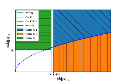
Figure 1: Visual representation of the various sums

We upper bound each of these sums separately.

Sum A.1:

We upper bound this term by $\lesssim\eta(k)\operatorname{\textsc{OPT}_{\ell_{0}}}\lesssim e^{-k}\operatorname{\textsc{OPT}_{\ell_{0}}}$.

From Lemma 5 we have that for $t\geq k$

$$f(t,w)\leq w\sqrt{\left\lceil\frac{t}{k}\right\rceil}\,\operatorname{\textsc{OPT}_{\ell_{0}}}\leq w\sqrt{\frac{2t}{k}}\,\operatorname{\textsc{OPT}_{\ell_{0}}},$$ (12)

and also $p(t,w)\leq\Pr(\|X\|_{2}=w)$. Thus, fixing $t$ and adding over $w\geq\sqrt{t}$ we get

$$\sum_{w\geq\sqrt{t}}f(t,w)\,p(t,w) \leq\operatorname{\textsc{OPT}_{\ell_{0}}}\,\sqrt{\frac{2t}{k}}\,\left(\sum_{w\geq\sqrt{t}}w\,\text{Pr}(\|X\|_{2}=w)\right).$$ (13)

Using Corollary 2 and the fact $t\geq k+1\geq 11$, the sum inside the bracket on the right-hand side of (13) is at most $c_{2}1.05\sqrt{t}\,e^{-t}$. Employing this bound on inequality (13) and adding over all $t\geq k+1$ we obtain

Sum A.1 $$\leq\left(c_{2}\frac{\sqrt{2}\cdot 1.05}{\sqrt{k}}\cdot\sum_{t\geq k+1}te^{-t}\right)\operatorname{\textsc{OPT}_{\ell_{0}}}\leq c_{2}\frac{3}{2\sqrt{k}}\eta(k+1)\operatorname{\textsc{OPT}_{\ell_{0}}},$$

where the final inequality follows from Lemma 1.

Sum A.2:

For $w\leq\sqrt{t}$, and using Lemma 5 we obtain

$$f(t,w)\leq t\sqrt{\frac{2}{k}}\,\operatorname{\textsc{OPT}_{\ell_{0}}},$$

and thus the sum A.2 can be upper bounded

$$\sum_{t\geq k+1}\sum_{w\leq\sqrt{t}}f(t,w)\,p(t,w) \leq\sqrt{\frac{2}{k}}\operatorname{\textsc{OPT}_{\ell_{0}}}\sum_{t\geq k+1}t\sum_{w\leq\sqrt{t}}p(t,w)$$

$$\leq\sqrt{\frac{2}{k}}\operatorname{\textsc{OPT}_{\ell_{0}}}\sum_{t\geq k+1}t\Pr\left(\|X\|_{0}=t\right)$$

$$\leq\sqrt{\frac{2}{k}}\operatorname{\textsc{OPT}_{\ell_{0}}}e^{c_{1}k-k-1}(k+2) \textrm{(Corollary \ref{cor:intl0})}.$$

Sum B:

For $t\leq k$, Lemma 5 gives that $f(t,w)\leq w\operatorname{\textsc{OPT}_{\ell_{0}}}$, and thus sum B can be upper bounded as

$$\sum_{t\leq k}\sum_{w\geq g}f(t,w)\,p(t,w) \leq\sum_{t\leq k}\sum_{w\geq g}w\operatorname{\textsc{OPT}_{\ell_{0}}}\cdot p(t,w)$$

$$\leq\operatorname{\textsc{OPT}_{\ell_{0}}}\sum_{w\geq g}w\Pr\left(\|X\|_{2}=w\right)$$

$$\leq c_{2}\left(g+\frac{1}{2g}\right)e^{-g^{2}}\operatorname{\textsc{OPT}_{\ell_{0}}} (\textrm{Corollary \ref{cor:intl2}}).$$

Employing these bounds on inequality (11) concludes the proof of the lemma. ∎

3.6 Conclusion of the Proof of Theorem 1

Taking a union bound, the probability that the $\frac{X}{g}$ is feasible is at least

$$1-\Pr(\|X\|_{0}\geq k+1)-\Pr(\|X\|_{2}\geq g).$$

One can verify that with the setting $\gamma=0.44$ and $g=2.69$, Lemma 6 and 7 imply that this quantity is strictly positive.

Moreover, combining equation (10) and Lemma 8, and using the fact that $\frac{X}{g}$ is feasible with non-zero probability, we have:

$$\mathbb{E}\bigg{[}\phi\bigg{(}\frac{X}{g}\bigg{)}~{}\bigg{|}~{}\bigg{\|}\frac{X}{g}\bigg{\|}_{0}\leq k,\bigg{\|}\frac{X}{g}\bigg{\|}_{2}\leq 1\bigg{]}\Pr\left(\bigg{\|}\frac{X}{g}\bigg{\|}_{0}\leq k,\bigg{\|}\frac{X}{g}\bigg{\|}_{2}\leq 1\right)\geq\frac{\textsc{OPT}_{\ell_{1}}-\alpha\operatorname{\textsc{OPT}_{\ell_{0}}}}{g}$$

$$\Rightarrow\mathbb{E}\bigg{[}\phi\bigg{(}\frac{X}{g}\bigg{)}~{}\bigg{|}~{}\bigg{\|}\frac{X}{g}\bigg{\|}_{0}\leq k,\bigg{\|}\frac{X}{g}\bigg{\|}_{2}\leq 1\bigg{]}\geq\frac{\textsc{OPT}_{\ell_{1}}-\alpha\operatorname{\textsc{OPT}_{\ell_{0}}}}{g}.$$

Therefore, there exists a scenario among the ones where $\frac{X}{g}$ is feasible where $\phi(\frac{X}{g})\geq\frac{\textsc{OPT}_{\ell_{1}}-\alpha\operatorname{\textsc{OPT}_{\ell_{0}}}}{g}$. Since $\operatorname{\textsc{OPT}_{\ell_{0}}}\geq\phi(\frac{X}{g})\geq\frac{\textsc{OPT}_{\ell_{1}}-\alpha\operatorname{\textsc{OPT}_{\ell_{0}}}}{g}$ implies $(g+\alpha)\operatorname{\textsc{OPT}_{\ell_{0}}}\geq\textsc{OPT}_{\ell_{1}}$. Verifying that with our setting of $g=2.69,\gamma=0.44,k=15$, we have $\operatorname{\textsc{OPT}_{\ell_{0}}}\geq\frac{1}{2.95}\textsc{OPT}_{\ell_{1}}$ concludes the proof of the first part of the theorem.

To prove the second part of the theorem, similar to the above, if the probability that the $\frac{X}{g}$ is feasible is positive, then we have that $\mathbb{E}[\phi(\frac{X}{g})|\frac{X}{g}\textup{ is feasible}]\geq\frac{\textsc{OPT}_{\ell_{1}}-\alpha\operatorname{\textsc{OPT}_{\ell_{0}}}}{g}$. Thus if the probability that the $\frac{X}{g}$ is feasible is positive, we obtain that with positive probability, $\frac{X}{g}$ is both feasible and satisfies $\phi(\frac{X}{g})\geq\frac{1-\alpha}{g}\textsc{OPT}_{\ell_{1}}$ (the last inequality follows from $\textsc{OPT}_{\ell_{0}}\leq\textsc{OPT}_{\ell_{1}}$). Setting $g=2.996$, $\gamma=0.4051$ for $k=15$, we have $\phi(\frac{X}{g})\geq\frac{1}{3.25}\textsc{OPT}_{\ell_{1}}$ which concludes the proof of the second part of the theorem.

4 Proof of Theorem 2

We begin with a simple observation.

Observation 1.

Suppose $A=(x^{*})(x^{*})^{T}$ where $x^{*}\in\mathbb{R}^{n}_{+}$, $\|x^{*}\|_{2}=1$, and $\|x^{*}\|_{1}\leq\sqrt{k}$, and consider the problems, Semi-norm SPCA and $\ell_{1}$-norm relaxation with objective function $\phi=\|.\|_{A}$. Then we have $\textsc{OPT}_{\ell_{1}}=1$. Moreover, if the coordinates of $x^{*}$ are sorted in non-increasing order, then $\textsc{OPT}_{\ell_{0}}=\sum_{i=1}^{k}x_{i}^{2}$.

Therefore, in order to find instances where the ratio $\frac{\textsc{OPT}_{\ell_{1}}}{\textsc{OPT}_{\ell_{0}}}$ is large, we can solve the following optimization problem:

$$\begin{array}[]{rcl}\textup{min}_{x}&\sum_{i=1}^{k}x_{i}^{2}&\\ \textup{s.t.}&\|x\|_{2}&=1\\ &\sum_{i=1}^{n}x_{i}&\leq\sqrt{k}\\ &-x_{i}+x_{i+1}&\leq 0,~{}i=1,\ldots,n-1\\ &-x_{n}&\leq 0,\end{array}$$ (19)

We show that this optimization problem can be reduced to a four variable optimization problem. In order to do so, note that the above problem is equivalent to the following problem:

$$\begin{array}[]{rcl}\textup{min}_{x,a,G,H,C,D}&G&\\ \textup{s.t.}&\sum_{i=1}^{k}x_{i}^{2}&=G\\ &\sum_{i=k+1}^{n}x_{i}^{2}&=H\\ &G+H&=1\\ &\sum_{i=1}^{k}x_{i}&=C\\ &\sum_{i=k+1}^{n}x_{i}&=D\\ &C+D&\leq\sqrt{k}\\ &x_{1},\ldots,x_{k}&\geq a\\ &x_{k+1},\ldots,x_{n}&\leq a\\ &x_{k+1},\ldots,x_{n}&\geq 0.\end{array}$$ (30)

In order to solve this problem we first determine some bounds on the new variables $a,G,H,C,D$.

Proposition 3.

Let $x,a,G,H,C,D$ be a feasible solution for (30). Then:

1. $a\geq 0$

2. $ka\leq C\leq\sqrt{k}$

3. $0\leq D\leq\sqrt{k}-C$

4. $\underbrace{\frac{D^{2}}{n-k}}_{H_{\text{Lower}}}\leq H\leq\underbrace{\left\lfloor\frac{D}{a}\right\rfloor a^{2}+\left(D-\left\lfloor\frac{D}{a}\right\rfloor a\right)^{2}}_{H_{\text{Upper}}}$, assuming $n-k\geq\lfloor\frac{D}{a}\rfloor+1$

5. $\underbrace{\frac{C^{2}}{k}}_{G_{\text{Lower}}}\leq G\leq\underbrace{(C-(k-1)a)^{2}+(k-1)a^{2}}_{G_{\text{Upper}}}$

Proof.

Items 1 through 3 follow directly from the constraints in (30).

Item 4. The upper bound comes from maximizing $\sum_{i=k+1}^{n}x_{i}^{2}$ subject to the condition $\sum_{i=k+1}^{n}x_{i}=D,\ x_{i}\in[0,\ a]\textup{ for all }i\in\{k+1,\dots,n\}$ (assuming $n-k\geq\lfloor\frac{D}{a}\rfloor+1$). The lower bound on $H$ is obtained by minimizing $\sum_{i=k+1}^{n}x_{i}^{2}$ subject to the condition $\sum_{i=k+1}^{n}x_{i}=D$. Note that the optimal solution is setting $x_{i}=\frac{D}{n-k}$ for all $x_{i}$, and under the assumption of $n-k\geq\lfloor\frac{D}{a}\rfloor+1$ each of these $x_{i}$’s is less than of equal to $a$.

Item 5. The upper bound comes from maximizing $\sum_{i=1}^{k}x_{i}^{2}$ subject to the condition $\sum_{i=1}^{k}x_{i}=C,\ x_{i}\geq a\textup{ for all }i\in[k]$. The lower bound on $G$ is obtained by minimizing $\sum_{i=1}^{k}x_{i}^{2}$ subject to the condition $\sum_{i=k+1}^{n}x_{i}=C$. ∎

Proposition 4.

Suppose there exists $a$, $C$, $D$ satisfying (1), (2), (3) of Proposition 3 such that $G_{\text{Upper}}+H_{\text{Upper}}\geq 1$. Let $G^{*}=\textup{max}\{G_{\text{Lower}},1-H_{\text{Upper}}\}$. Then exists a vector $x\in\mathbb{R}^{n}_{+}$ satisfying the feasible region of (30) with objective function value equal to $G^{*}$.

Proof.

Note that since $G_{\text{Upper}}+H_{\text{Upper}}\geq 1$, $G^{*}=\textup{max}\{G_{\text{Lower}},1-H_{\text{Upper}}\}$ is the smallest value in the interval $[G_{\text{Lower}},\ G_{\text{Upper}}]$ such that there exists $H^{*}\in[H_{\text{Lower}},\ H_{\text{Upper}}]$ satisfying $G^{*}+H^{*}=1$.

Via the proof of Proposition 3, there exists a solution $x_{\text{Upper}}\in\mathbb{R}^{n-k}_{+}$ satisfying, $\|x_{\text{Upper}}\|_{2}=H_{\text{Upper}}$, $\|x_{\text{Upper}}\|_{1}=D$, and $(x_{\text{Upper}})_{i}\leq a\ \forall i\in[n-k]$. Similarly, there exists a solution $x_{\text{Lower}}\in\mathbb{R}^{n-k}_{+}$ satisfying, $\|x_{\text{Lower}}\|_{2}=H_{\text{Lower}}$, $\|x_{\text{Lower}}\|_{1}=D$, and $(x_{\text{Lower}})_{i}\leq a\ \forall i\in[n-k]$. Since $\|\cdot\|_{2}$ is a continuous function there is a convex combination of $x_{\text{Upper}}$ and $x_{\text{Lower}}$, say $y\in\mathbb{R}^{n-k}_{+}$ satisfying $\|y\|_{2}=H^{*}$, $\|y\|_{1}=D$, and $(y)_{i}\leq a\ \forall i\in[n-k]$.

Now using the same argument for $G$, we can obtain $z\in\mathbb{R}^{k}_{+}$ such that $\|z\|_{2}=G^{*}$, $\|z\|_{1}=C$, and $(z)_{i}\geq a\ \forall i\in[n-k]$. Thus, the augmented vector, $(z^{\top}\ y^{\top})^{\top}$ satisfies the feasible region of (30) with objective function value equal to $G^{*}$. ∎

As a consequence of Proposition 4, the optimization problem (19) may be solved by solving the following problem:

$$\begin{array}[]{rl}\textup{min}_{\theta,a,C,D}&\theta\\ \textup{s.t.}&\frac{1}{\sqrt{k}}\geq a\geq 0\\ &\sqrt{k}\geq C\geq ka\\ &\sqrt{k}-C\geq D\geq 0\\ &\left\lfloor\frac{D}{a}\right\rfloor a^{2}+\left(D-\left\lfloor\frac{D}{a}\right\rfloor a\right)^{2}+(C-(k-1)a)^{2}+(k-1)a^{2}\geq 1\\ &\theta\geq\frac{C^{2}}{k}\\ &\theta\geq 1-\left(\left\lfloor\frac{D}{a}\right\rfloor a^{2}+\left(D-\left\lfloor\frac{D}{a}\right\rfloor a\right)^{2}\right)\end{array}$$ (38)

Note in the above problem, we can always set $D=\sqrt{k}-C$. We solved the above problem numerically (obtaining an upper bound to (30)), by just discretizing in the space of $a$ and $C$ variables and taking the best feasible point. The result of our numerical experiments is presented in Figure 2, where the $y$-axis is the reciprocal of the optimal objective function value of problem (38), which is $\textsc{OPT}_{\ell_{1}}/\textsc{OPT}_{\ell_{0}}$. Notice that $\textsc{OPT}_{\ell_{1}}/\textsc{OPT}_{\ell_{0}}$ is increasing with increasing values of $k$, but it seems to converge to a value slightly greater than $1.32$. It can be verified that $k=10000$, $a=0.005$, $C=51$, $D=49$, $\theta=0.755$ is a feasible solution for (38), i.e. $\textsc{OPT}_{\ell_{1}}/\textsc{OPT}_{\ell_{0}}\geq 1.324$. This completes the proof of Theorem 2.

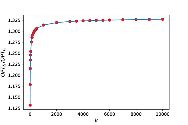
Figure 2: Result of Problem (38) for varying values of $k$

Acknowledgements.

Santanu S. Dey would like to acknowledge the support of NSF CMMI grant 1562578.

Appendix

Appendix A Proof of Lemma 3

Using Markov’s inequality and independence we have

$$\text{Pr}\left(\sum_{i}X_{i}\geq t\right) =\text{Pr}\left(e^{\sum_{i}X_{i}}\geq e^{t}\right)\leq\frac{\mathbb{E}e^{\sum_{i}X_{i}}}{e^{t}}=\frac{\prod_{i}\mathbb{E}e^{X_{i}}}{e^{t}}.$$ (39)

But for $x\in[0,b_{i}]$ we have $e^{x}\leq 1+x\frac{e^{b_{i}}-1}{b_{i}}$; furthermore, $e^{y}\leq 1+y+(e-2)y^{2}$ for $y\in[0,1]$, so employing this to bound $e^{b_{i}}$ in the previous inequality we obtain $e^{x}\leq 1+x(1+(e-2)b_{i})$. Therefore,

$$\mathbb{E}e^{X_{i}}\leq 1+\mu_{i}(1+(e-2)b_{i})\leq e^{\mu_{i}(1+(e-2)b_{i})},$$

where the last inequality follows from $1+x\leq e^{x}$ that holds for all $x$. Employing this bound on (39) concludes the proof of the lemma.

References

• [1] T. W. Anderson. An Introduction to Multivariate Statistical Analysis. Wiley, New York, 3rd edition, 2003.
• [2] Aharon Birnbaum, Iain M Johnstone, Boaz Nadler, and Debashis Paul. Minimax bounds for sparse pca with noisy high-dimensional data. Annals of statistics, 41(3):1055, 2013.
• [3] Stéphane Boucheron, Gábor Lugosi, and Pascal Massart. Concentration inequalities: A nonasymptotic theory of independence. Oxford university press, 2013.
• [4] Peter Bühlmann and Sara van-de-Geer. Statistics for high-dimensional data. Springer, 2011.
• [5] Jorge Cadima and Ian T Jolliffe. Loading and correlations in the interpretation of principle compenents. Journal of Applied Statistics, 22(2):203–214, 1995.
• [6] Emmanuel J Candes, Justin K Romberg, and Terence Tao. Stable signal recovery from incomplete and inaccurate measurements. Communications on pure and applied mathematics, 59(8):1207–1223, 2006.
• [7] Emmanuel J Candes and Terence Tao. Decoding by linear programming. IEEE transactions on information theory, 51(12):4203–4215, 2005.
• [8] A. d’Aspremont, L. El. Ghaoui, M. I. Jordan, and G. R. G. Lanckriet. A direct formulation for sparse pca using semidefinite programming. SIAM Review, 49:434–448, 2007.
• [9] D. Donoho. For most large underdetermined systems of equations, the minimal $\ell^{1}$-norm solution is the sparsest solution. Communications on Pure and Applied Mathematics, 59:797–829, 2006.
• [10] Willliam Feller. An introduction to probability theory and its applications, volume 2. John Wiley & Sons, 2008.
• [11] Kimon Fountoulakis, Abhisek Kundu, Eugenia-Maria Kontopoulou, and Petros Drineas. A randomized rounding algorithm for sparse PCA. TKDD, 11(3):38:1–38:26, 2017.
• [12] G. Golub and C. Van Loan. Matrix Computations. Johns Hopkins University Press, Baltimore., 1983.
• [13] Peter JB Hancock, A Mike Burton, and Vicki Bruce. Face processing: Human perception and principal components analysis. Memory & Cognition, 24(1):26–40, 1996.
• [14] Trevor Hastie, Robert Tibshirani, Michael B Eisen, Ash Alizadeh, Ronald Levy, Louis Staudt, Wing C Chan, David Botstein, and Patrick Brown. ’gene shaving’as a method for identifying distinct sets of genes with similar expression patterns. Genome biology, 1(2):research0003–1, 2000.
• [15] Trevor Hastie, Robert Tibshirani, and Jerome Friedman. The Elements of Statistical Learning, Second Edition: Data Mining, Inference, and Prediction. Springer New York, 2 edition, 2009.
• [16] Trevor Hastie, Robert Tibshirani, and Martin Wainwright. Statistical learning with sparsity. CRC press, 2015.
• [17] Harold Hotelling. Analysis of a complex of statistical variables into principal components. Journal of educational psychology, 24(6):417, 1933.
• [18] Rodolphe Jenatton, Guillaume Obozinski, and Francis Bach. Structured sparse principal component analysis. In Proceedings of the Thirteenth International Conference on Artificial Intelligence and Statistics, pages 366–373, 2010.
• [19] Iain M Johnstone and Arthur Yu Lu. On consistency and sparsity for principal components analysis in high dimensions. Journal of the American Statistical Association, 104(486):682–693, 2009.
• [20] Ian T Jolliffe. Principal component analysis and factor analysis. Principal component analysis, pages 150–166, 2002.
• [21] Ian T Jolliffe, Nickolay T Trendafilov, and Mudassir Uddin. A modified principal component technique based on the lasso. Journal of computational and Graphical Statistics, 12(3):531–547, 2003.
• [22] Michel Journée, Yurii Nesterov, Peter Richtárik, and Rodolphe Sepulchre. Generalized power method for sparse principal component analysis. Journal of Machine Learning Research, 11(Feb):517–553, 2010.
• [23] Elliott H Lieb and Michael Loss. Analysis, volume 14 of graduate studies in mathematics. American Mathematical Society, Providence, RI,, 4, 2001.
• [24] Ronny Luss and Marc Teboulle. Conditional gradient algorithmsfor rank-one matrix approximations with a sparsity constraint. SIAM Review, 55(1):65–98, 2013.
• [25] Michael McCoy, Joel A Tropp, et al. Two proposals for robust pca using semidefinite programming. Electronic Journal of Statistics, 5:1123–1160, 2011.
• [26] Jatin Misra, William Schmitt, Daehee Hwang, Li-Li Hsiao, Steve Gullans, George Stephanopoulos, and Gregory Stephanopoulos. Interactive exploration of microarray gene expression patterns in a reduced dimensional space. Genome research, 12(7):1112–1120, 2002.
• [27] Nikhil Naikal, Allen Y Yang, and S Shankar Sastry. Informative feature selection for object recognition via sparse PCA. In Computer Vision (ICCV), 2011 IEEE International Conference on, pages 818–825. IEEE, 2011.
• [28] Debashis Paul and Iain M Johnstone. Augmented sparse principal component analysis for high dimensional data. arXiv preprint arXiv:1202.1242, 2012.
• [29] Haipeng Shen and Jianhua Z Huang. Sparse principal component analysis via regularized low rank matrix approximation. Journal of multivariate analysis, 99(6):1015–1034, 2008.
• [30] R. Tibshirani. Regression shrinkage and selection via the lasso. Journal of the Royal Statistical Society, Series B, 58:267–288, 1996.
• [31] Harun Uğuz. A two-stage feature selection method for text categorization by using information gain, principal component analysis and genetic algorithm. Knowledge-Based Systems, 24(7):1024–1032, 2011.
• [32] Vincent Q Vu and Jing Lei. Minimax rates of estimation for sparse pca in high dimensions. In International Conference on Artificial Intelligence and Statistics, pages 1278–1286, 2012.
• [33] DM. Witten, R. Tibshirani, and T. Hastie. A penalized matrix decomposition, with applications to sparse principal components and canonical correlation analysis. Biostatistics, 10(3):515–534, 2009.
• [34] Youwei Zhang, Alexandre d’Aspremont, and Laurent El Ghaoui. Sparse PCA: Convex relaxations, algorithms and applications. In Handbook on Semidefinite, Conic and Polynomial Optimization, pages 915–940. Springer, 2012.
• [35] P. Zhao and B. Yu. On model selection consistency of lasso. Journal of Machine Learning Research, 7:2541–2563, 2006.
• [36] Hui Zou, Trevor Hastie, and Robert Tibshirani. Sparse principal component analysis. Journal of computational and graphical statistics, 15(2):265–286, 2006.