Abstract

Two-Higgs-doublet models (2HDMs) are minimal extensions of the Standard Model (SM) that may still be discovered at the LHC. The quartic couplings of their potentials can be determined from the measurement of the masses and branching ratios of their extended scalar sectors. We show that the evolution of these couplings through renormalization group equations can determine whether the observed 2HDM is a low energy manifestation of a more fundamental theory, as for instance, supersymmetry, which fixes the quartic couplings in terms of the gauge couplings. At leading order, the minimal supersymmetric extension of the SM (MSSM) dictates all the quartic couplings, which can be translated into a predictive structure for the scalar masses and mixings at the weak scale. Running these couplings to higher scales, one can check if they converge to their MSSM values, and more interestingly, whether one can infer the supersymmetry breaking scale. Although we study this question in the context of supersymmetry, this strategy could be applied to any theory whose ultraviolet completion unambiguously predicts all scalar quartic couplings.

1 Introduction

Despite several theoretical and experimental motivations for new physics beyond the standard model (BSM), the LHC data on the production and branching ratios of the Higgs boson are tantalizingly close to their SM predictions [1, 2, 3, 4], yet to reveal any convincing sign of life beyond it. Although it is entirely possible that no new physics exists between the electroweak and the grand unification or Planck scales, modulo some dark matter source, this grand desert scenario carries with it many unpleasant features such as the hierarchy between the electroweak and Planck scale, lack of gauge unification, etc.

From a rather pragmatic point of view, a vital question in motivating collider searches for BSM physics above the electroweak scale (EWS) is whether we can foretell the approximate mass range where new particles are expected to appear. This is precisely the hurdle most new physics models fail to cross. Predicting the existence of many new particles, most such models provide guidance on what to look for, leaving no clue, unfortunately, on where. Therefore, any principle that gives some idea of the probable mass scales of the new particles deserves special attention from a phenomenological point of view. The present article is an attempt in this direction.

Amongst the vast array of BSM scenarios, extensions of the SM scalar sector have been explored with various motivations, e.g. for generating the necessary additional CP violation to account for the observed baryon asymmetry of the universe. In these models, the 125 GeV Higgs boson just happens to be one of the scalars in the spectrum, the others yet to be discovered. Phenomenologically, 2HDMs provide one of the simplest realizations in this category, wherein the scalar sector of the SM is augmented by just one additional doublet [5, 6]. Aside from their simplicity, these models have the desirable property that the oblique electroweak $\rho$-parameter remains unity at the tree level, along with providing an alignment limit [7, 8, 9, 10, 11], where a SM-like Higgs can be recovered. Quite notably, the MSSM [12, 13, 14, 15, 16, 17] is structured around two such Higgs doublets.

In view of the increasing affinity of the LHC Higgs data to the SM-predicted values, the ability to attain the alignment limit might hold the key for future survival of any such new physics model. Let us suppose that the only hint of new physics from forthcoming data somehow points towards a 2HDM structure, either directly or indirectly. If the 2HDM is viewed as an effective low-energy model arising from a more fundamental ultraviolet (UV) theory, it would be interesting to ask whether the knowledge of the 2HDM potential at LHC scales can give us any hint of its embedding in a particular UV scenario, containing massive states sitting at an inaccessibly high scale.

Under the assumption of CP conservation, 2HDMs predict the existence of five physical scalars: two CP-even ($h$ and $H$), one CP-odd ($A$) and a pair of charged scalars ($H^{\pm}$). We assume that the lightest CP-even scalar ($h$) is the one already discovered with a mass $\sim 125$ GeV. Its SM-like properties, as LHC data indicate, compel us to stay close to the alignment limit. However, it is still possible that the nonstandard scalars might all be lurking below the TeV scale waiting to be discovered at the LHC. In that case, we would, in principle, be able to measure all the parameters of the 2HDM scalar potential. By studying the renormalization group (RG) evolution of these parameters, we would then be able to test whether the 2HDM is a low energy manifestation of a more fundamental theory with an enhanced symmetry at a high scale, $\Lambda_{S}$.

In this paper, we focus our attention on the MSSM framework as a well motivated example in this category. A high supersymmetry (SUSY) breaking scale may seem to run contrary to the common lore of its solution to the hierarchy problem and arriving at the correct $125$ GeV mass for the light Higgs. Nevertheless, viewed as a 2HDM effective theory, achieving the correct mass for the Higgs can be translated into obtaining the correct value for its quartic couplings when matched and run down from $\Lambda_{S}$ to the EWS. Indeed, such “High Scale SUSY” scenarios have been studied before in the literature, both in the case where the effective theory below the SUSY scale is strictly the SM [18, 19, 20, 21, 22], or a 2HDM in the context of a moderately high SUSY scale $\Lambda_{S}\sim 10^{4}$ GeV [23, 24, 25, 26, 27]. It was found that, in both scenarios, solutions indeed exist for low values of $\tan\beta$. Larger values of $\Lambda_{S}$ have also been considered in [28, 29, 30, 31] where the 2HDM spectrum was obtained by matching the 2HDM to the MSSM at the $\Lambda_{S}$ scale and running it down to the EWS. These studies have been done using state of the art calculations (matching at one loop plus dominant two loops, and running at two loops). On the contrary, here we follow a bottom-up approach by assuming that the spectrum of scalar masses and mixings will be measured at the EWS from where the scalar potential can be determined. Then, we run the quartic couplings of the potential, using the 2HDM Renormalization Group Equations (RGE) [32, 33, 34] as implemented by SARAH 4 [35], and check if they satisfy the SUSY boundary conditions at a higher scale, as usually done in Grand Unified Theories. This approach has the advantage that it is independent of the details of the underlying theory which are hidden in the matching conditions at the high scale.

2 Effective 2HDMs and parameter counting

The most general gauge invariant potential built with two SU(2) doublet scalars (with hypercharge $Y=+1$), $\phi_{1}$ and $\phi_{2}$, can be written as[7]

$$V = m_{11}^{2}\phi_{1}^{\dagger}\phi_{1}+m_{22}^{2}\phi_{2}^{\dagger}\phi_{2}-\left(m_{12}^{2}\phi_{1}^{\dagger}\phi_{2}+{\rm h.c.}\right)$$ (1)

$$+ \frac{\lambda_{1}}{2}\left(\phi_{1}^{\dagger}\phi_{1}\right)^{2}+\frac{\lambda_{2}}{2}\left(\phi_{2}^{\dagger}\phi_{2}\right)^{2}+\lambda_{3}\left(\phi_{1}^{\dagger}\phi_{1}\right)\left(\phi_{2}^{\dagger}\phi_{2}\right)+\lambda_{4}\left(\phi_{1}^{\dagger}\phi_{2}\right)\left(\phi_{2}^{\dagger}\phi_{1}\right)$$

$$+ \left[\frac{\lambda_{5}}{2}\left(\phi_{1}^{\dagger}\phi_{2}\right)^{2}+\left(\lambda_{6}\left(\phi_{1}^{\dagger}\phi_{1}\right)+\lambda_{7}\left(\phi_{2}^{\dagger}\phi_{2}\right)\right)\left(\phi_{1}^{\dagger}\phi_{2}\right)+{\rm h.c.}\right]\,.$$

This potential contains 3 mass parameters and 7 quartic couplings, understood as $\overline{\rm MS}$ parameters at the EWS arising from a more complete theory at higher energies. If $m_{12},\lambda_{5},\lambda_{6},\lambda_{7}$ are all zero, the potential has an additional U(1) global symmetry [36]. If only $m_{12},\lambda_{6},\lambda_{7}$ are zero the U(1) is broken but there remains an unbroken discrete $Z_{2}$ symmetry. If only $\lambda_{6},\lambda_{7}$ are zero, then this discrete symmetry is softly broken by $m_{12}$. Models in which this $Z_{2}$ is also preserved by the Yukawa couplings (with $\phi_{1}$ coupled only to down-type fermions and $\phi_{2}$ only to up-type fermions) are called type II 2HDMs. This discrete symmetry is useful for avoiding large flavor changing neutral currents and appears, as an approximate symmetry, in supersymmetric models.

We assume that all the parameters in the potential are real. After electroweak spontaneous symmetry breaking (SSB), one obtains the physical spectrum, specified by seven parameters: the four physical scalar masses ($m_{h}$, $m_{H}$, $m_{A}$ and $m_{+}$), the total vacuum expectation value (vev) $v=\sqrt{v_{1}^{2}+v_{2}^{2}}$, $\tan\beta=v_{2}/v_{1}$, and the alignment angle $\cos(\beta-\alpha)$ (here $\alpha$ is the mixing angle in the CP-even sector).

In principle, the whole spectrum can be determined from knowledge of the quartic couplings. Consider the situation where all the quartic couplings in Eq. (1) are known (from some symmetry principle, e.g. supersymmetry) at a scale $\Lambda_{S}$. Then the remaining three bilinear parameters can be solved from the knowledge of $v$ ($=246$ GeV), $m_{h}$ ($\simeq 125$ GeV) and $\tan\beta$ (or alternatively $\cos(\beta-\alpha)$). In other words, the complete 2HDM spectrum is then determined modulo the experimental uncertainties in the quoted parameters. Explicitly, the SSB contributions to the charged scalar masses and to the mass matrix of the neutral scalars in the Higgs basis can be written solely in terms of the $\lambda_{i}$ and $\tan\beta$, as follows (see [28, 37] for details):

$$g_{11} = \lambda_{1}\cos^{4}\beta+\lambda_{2}\sin^{4}\beta+2\left(\lambda_{3}+\lambda_{4}+\lambda_{5}\right)\sin^{2}\beta\cos^{2}\beta+4\lambda_{6}\cos^{3}\beta\sin\beta+4\lambda_{7}\sin^{3}\beta\cos\beta\,,$$ (2a)

$$g_{12} = \cos\beta\sin\beta\left(\lambda_{2}\sin^{2}\beta-\lambda_{1}\cos^{2}\beta+\left(\lambda_{3}+\lambda_{4}+\lambda_{5}\right)\cos 2\beta\right)$$ (2b)

$$+3(\lambda_{7}-\lambda_{6})\sin^{2}\beta\cos^{2}\beta+\lambda_{6}\cos^{4}\beta-\lambda_{7}\sin^{4}\beta\,,$$

$$g_{22} = \left(\lambda_{1}+\lambda_{2}\right)\cos^{2}\beta\sin^{2}\beta-2\left(\lambda_{3}+\lambda_{4}\right)\cos^{2}\beta\sin^{2}\beta$$ (2c)

$$+\lambda_{5}(\sin^{4}\beta+\cos^{4}\beta)+(\lambda_{7}-\lambda_{6})\sin 2\beta\cos 2\beta\,,$$

$$g_{+} = \frac{1}{2}\left(\lambda_{5}-\lambda_{4}\right)\,.$$ (2d)

The diagonalization of the mass terms leads to

$$g_{11}v^{2} = m_{H}^{2}\cos^{2}(\beta-\alpha)+m_{h}^{2}\sin^{2}(\beta-\alpha)\,,$$ (3a)

$$g_{22}v^{2} = m_{H}^{2}\sin^{2}(\beta-\alpha)+m_{h}^{2}\cos^{2}(\beta-\alpha)-m_{A}^{2}\,,$$ (3b)

$$g_{12}v^{2} = \left(m_{h}^{2}-m_{H}^{2}\right)\cos(\beta-\alpha)\sin(\beta-\alpha)\,,$$ (3c)

$$g_{+}v^{2} = m_{+}^{2}-m_{A}^{2}\,,$$ (3d)

which, when inverted, yield (in terms of the known $m_{h}$ and $v$)

$$m_{H}^{2} = g_{11}v^{2}+\frac{\left(g_{12}v^{2}\right)^{2}}{g_{11}v^{2}-m^{2}_{h}}\,,$$ (4a)

$$m_{A}^{2} = m_{h}^{2}-g_{22}v^{2}+\frac{\left(g_{12}v^{2}\right)^{2}}{g_{11}v^{2}-m^{2}_{h}}\,,$$ (4b)

$$m_{+}^{2} = m_{h}^{2}-g_{22}v^{2}+\frac{\left(g_{12}v^{2}\right)^{2}}{g_{11}v^{2}-m^{2}_{h}}+g_{+}v^{2}\,,$$ (4c)

$$\cos\left(\beta-\alpha\right) = -~{}\mathrm{sgn}(g_{12})\bigg{/}\sqrt{1+\left(\frac{g_{12}v^{2}}{g_{11}v^{2}-m^{2}_{h}}\right)^{2}}\,.$$ (4d)

The above equations explicitly show how the scalar masses and mixings can be obtained, once all $\lambda_{i}$ are known, in terms of $v$, $m_{h}$ and $\tan\beta$.

Assuming that all supersymmetric particles are much heavier than the EWS, the MSSM provides a perfect example of a model where the Higgs sector is a 2HDM. In this case, the Higgs quartic couplings come from the supersymmetric $D$-terms and, at tree level, are simple functions of the gauge couplings [13, 38]:

$$\lambda_{1}=\lambda_{2}=\frac{1}{4}\left(g^{2}+g_{Y}^{2}\right)\,,~{}~{}\lambda_{3}=\frac{1}{4}\left(g^{2}-g_{Y}^{2}\right)\,,~{}~{}\lambda_{4}=-\frac{g^{2}}{2}\,,~{}~{}\lambda_{5}=\lambda_{6}=\lambda_{7}=0\,,$$ (5)

where $g$ and $g_{Y}$ are the ${\rm SU(2)_{W}}$ and ${\rm U(1)_{Y}}$ gauge couplings, respectively. Note that all mass terms are also generated at tree level. In particular, the $m_{12}$ term, which breaks the discrete $Z_{2}$ symmetry softly, is related to the bilinear $B\mu$ term in the SUSY potential. Therefore, at tree level, the MSSM leads to a type II 2HDM. The relations of Eq. (5) should be understood to hold at a scale $\Lambda_{S}$, where the general 2HDM is matched to the MSSM. Below $\Lambda_{S}$, the RG evolution of the 2HDM parameters should be used to obtain the potential at the EWS. Since the boundary condition $\lambda_{5}=\lambda_{6}=\lambda_{7}=0$ increases the symmetry of the quartic part of the Lagrangian, these couplings will not be generated by the RG evolution and will still be zero at lower energies.

This simple picture is perturbed if we consider the higher-order corrections to the Higgs potential. In the MSSM, the $Z_{2}$ symmetry is broken by the $\mu$-term in the superpotential ($\mu$ being the Higgsino mass parameter), and this breaking affects the higher order matching of all the $\lambda_{i}$ at the scale $\Lambda_{S}$. In particular, $\lambda_{5,6,7}(\Lambda_{S})$ will arise at higher loops but will always be proportional, at least, to $\mu/\Lambda_{S}$ [39], which we will consider to be small. Then, as RG evolution cannot generate them, it is reasonable to assume $\lambda_{5}\simeq\lambda_{6}\simeq\lambda_{7}\simeq 0$.

Similarly, the effective couplings $\lambda_{i}(i=1,\dots,4)$ in Eq. (5) receive corrections at the scale $\Lambda_{S}$ that depend on the full supersymmetric spectrum. These corrections are, however, sub-leading. In fact, the corrections proportional to the large third generation Yukawa couplings come with a factor of $\mu/\Lambda_{S}$ or $A_{t,b}/\Lambda_{S}$, $A_{t,b}$ being the trilinear soft-breaking terms. In the following, we assume that $\mu/\Lambda_{S},A_{t,b}/\Lambda_{S}\ll 1$, and thus these corrections as well as the smaller gauge corrections can be safely neglected.

Under these assumptions, we have only four quartic couplings, which can be determined from the scalar masses and mixings by inverting Eqs. (2a)–(2d) and using Eq. (3) as follows,

$$\lambda_{1} = g_{11}+g_{22}\tan^{2}\beta-2g_{12}\tan\beta\,,$$ (6a)

$$\lambda_{2} = g_{11}+g_{22}\cot^{2}\beta+2g_{12}\cot\beta\,,$$ (6b)

$$\lambda_{3} = g_{11}-g_{22}+2g_{12}\cot\left(2\beta\right)+2g_{+}\,,$$ (6c)

$$\lambda_{4} = -2g_{+}\,.$$ (6d)

Once these couplings are determined at the EWS, including appropriate radiative corrections[27, 40], we can use the 2HDM RGE to check whether their values correspond to the MSSM boundary conditions at a high scale.

3 RG analysis and pointers to high scale SUSY

To obtain a qualitative understanding of the RG evolution, we can begin by simply using the one loop RGE, checking the stability of these results under higher order corrections a posteriori. At one loop, the RG evolution of the gauge couplings is very simple and can be easily integrated. We will be interested here in the combination $(g^{2}+g_{Y}^{2})/4$ which, in a supersymmetric framework, would fix the boundary values for $\lambda_{1}$ and $\lambda_{2}$. The RG evolution of this combination at one loop is given by,

$${\cal D}(g^{2}+g_{Y}^{2})=\frac{-3g^{4}+7g_{Y}^{4}}{8\pi^{2}}\,,$$ (7)

where ${\cal D}\equiv d/d(\log M)$. Substituting their EWS values, we obtain $\left.(-3g^{4}+7g_{Y}^{4})/(8\pi^{2})\right|_{M_{z}}\simeq 0.003$, i.e. this combination remains essentially constant at one loop. On the other hand, the one loop RGE for the quartic couplings depend on the gauge as well as Yukawa couplings as follows [5]:

$${\cal D}\lambda_{1} = \frac{1}{16\pi^{2}}\bigg{[}\frac{3}{4}\left(3g^{4}+g_{Y}^{4}+2g^{2}g_{Y}^{2}\right)-3\lambda_{1}\left(3g^{2}+g_{Y}^{2}\right)$$ (8a)

$$+12\lambda_{1}^{2}+4\lambda_{3}^{2}+4\lambda_{3}\lambda_{4}+2\lambda_{4}^{2}+4\lambda_{1}\left(3y_{b}^{2}+y_{\tau}^{2}\right)-12y_{b}^{4}-4y_{\tau}^{4}\bigg{]}\,,$$

$${\cal D}\lambda_{2} = \frac{1}{16\pi^{2}}\bigg{[}\frac{3}{4}\left(3g^{4}+g_{Y}^{4}+2g^{2}g_{Y}^{2}\right)-3\lambda_{2}\left(3g^{2}+g_{Y}^{2}\right)$$ (8b)

$$+12\lambda_{2}^{2}+4\lambda_{3}^{2}+4\lambda_{3}\lambda_{4}+2\lambda_{4}^{2}+12\lambda_{2}y_{t}^{2}-12y_{t}^{4}\bigg{]}\,,$$

$${\cal D}\lambda_{3} = \frac{1}{16\pi^{2}}\bigg{[}\frac{3}{4}\left(3g^{4}+g_{Y}^{4}-2g^{2}g_{Y}^{2}\right)-3\lambda_{3}\left(3g^{2}+g_{Y}^{2}\right)$$ (8c)

$$+2\left(\lambda_{1}+\lambda_{2}\right)\left(3\lambda_{3}+\lambda_{4}\right)+4\lambda_{3}^{2}+2\lambda_{4}^{2}+2\lambda_{3}\left(3y_{t}^{2}+3y_{b}^{2}+y_{\tau}^{2}\right)-12y_{t}^{2}y_{b}^{2}\bigg{]}\,,$$

$${\cal D}\lambda_{4} = \frac{1}{16\pi^{2}}\bigg{[}3g^{2}g_{Y}^{2}-3\lambda_{4}\left(3g^{2}+g_{Y}^{2}\right)$$ (8d)

$$+2\left(\lambda_{1}+\lambda_{2}+4\lambda_{3}\right)\lambda_{4}+4\lambda_{4}^{2}+2\lambda_{4}\left(3y_{t}^{2}+3y_{b}^{2}+y_{\tau}^{2}\right)+12y_{t}^{2}y_{b}^{2}\bigg{]}\,,$$

where, $y_{f}$ stands for the Yukawa coupling of the fermion $f\,(=t,b,\tau)$. From these equations we see that only $\lambda_{2}$ should have significant evolution due to the large top Yukawa coupling, $y_{t}\sim{\cal O}\left(m_{t}/(v\sin\beta\right))$. This is true for $\tan\beta\sim$ 1–3, which is the relevant range for high scale SUSY, as we will see below. In particular, Eq. (5) implies that at the SUSY scale, we have $\lambda_{1}=\lambda_{2}=-(\lambda_{3}+\lambda_{4})=(g^{2}+g_{Y}^{2})/4$, and we can naturally expect that at lower scales $\lambda_{1}$ and $-(\lambda_{3}+\lambda_{4})$ will not deviate much from their boundary value, $(g^{2}+g_{Y}^{2})/4$, while $\lambda_{2}$ can be expected to grow significantly.

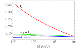
Figure 1: Two-loop RG evolution of $\lambda_{1}$, $\lambda_{2}$ and $-(\lambda_{3}+\lambda_{4})$ starting from supersymmetric boundary values at $\Lambda_{S}=10^{5}$ GeV with $\tan\beta=2.8$ (left panel), and $\Lambda_{S}=10^{10}$ GeV with $\tan\beta=1.7$ (right panel), as compared to the evolution of $(g^{2}+g_{Y}^{2})/4$ (dashed line).

We can observe this behavior in Fig. 1, where we have used two loop RGE to obtain the $\lambda_{i}$ values at the EWS starting from supersymmetric boundary values at $\Lambda_{S}=10^{5}$ GeV (left panel) and $\Lambda_{S}=10^{10}$ GeV (right panel). Note that we used the two loop RGE for the top quark Yukawa coupling because there is an accidental cancellation in the one loop beta function for $\tan\beta\sim 0.75$ which makes the two loop contributions relevant. One can already see this in the SM running of the top Yukawa coupling, ${\cal D}y_{t}^{\rm SM}\sim y_{t}^{\rm SM}\left\{4.5(y_{t}^{\rm SM})^{2}-8g_{s}^{2}\right\}$, which vanishes for $y_{t}^{\rm SM}=4g_{s}/3$, where $g_{s}$ is the gauge coupling for strong interaction. Strictly within the SM framework, this numerical situation never arises. In the 2HDM, however, the corresponding relation is $y_{t}^{\rm SM}/\sin\beta=4g_{s}/3$. This implies that in the vicinity of $\sin\beta\sim 0.6$, i.e., $\tan\beta\sim 0.75$, the one loop contributions to the beta function can be overshadowed by the two loop ones.

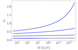
Figure 2: Evolution of $\lambda_{1}$ for different initial values ( from bottom to top, $\lambda_{1}=0.10,0.25,0.40,0.55$), as compared with $(g^{2}+g_{Y}^{2})/4$ (dashed line), for $\tan\beta=1.7$.

In Fig. 1 we showed that starting from small values ($\lambda_{1}\sim g^{2},g^{2}_{Y}$) $\lambda_{1}$ does not run much from $\Lambda_{S}$ to the EWS, and stays small. Now in a bottom-up approach one may wonder if this is also true when starting with larger values of $\lambda_{1}$ at the EWS and evolving it up to $\Lambda_{S}$. This evolution is shown in Fig. 2. With respect to the other quartic couplings, we take their initial EWS values to be: $\lambda_{2}=0.56$, $\lambda_{3}=0.015$ and $\lambda_{4}=-0.16$. Note, the evolution of $\lambda_{1}$ is independent of $\lambda_{2}$ at one loop. With regards to $\lambda_{3}$ and $\lambda_{4}$, we take the relatively small values corresponding to the gauge boundary conditions at the high scale. We see that, indeed, $\lambda_{1}$ evolves very little for small values of $\lambda_{1}$ at the EWS, $\lambda_{1}\leq 0.40$, and this result is, in practice, independent of $\tan\beta$ for $\tan\beta\leq 10$. Moreover $\lambda_{1}$ grows with the scale, and therefore, at the EWS, we should expect its value to be slightly smaller than $(g^{2}+g_{Y}^{2})/4\simeq 0.15$, if it is indeed determined by gauge couplings at the high scale.

From this discussion we can infer that a measurement of the quartic couplings of the Higgs potential at the EWS can favor a high scale SUSY scenario if the following features are observed:

• The values of $\lambda_{1}$ and $-(\lambda_{3}+\lambda_{4})$, at the EWS, are in the vicinity of $(g^{2}+g_{Y}^{2})/4\simeq 0.14$.

• The value of $\lambda_{2}$ should then be significantly larger than $(g^{2}+g_{Y}^{2})/4$, due to the large negative contribution to the RGE from the top Yukawa coupling.

• We can get a qualitative estimate of the SUSY scale, $\Lambda_{S}$, as the scale where $\lambda_{2}$ reaches its high scale boundary value, $(g^{2}+g_{Y}^{2})/4$.

• If $\lambda_{1}$ (or $-(\lambda_{3}+\lambda_{4})$) at the EWS is found to be larger than $\sim 0.4$, it will be impossible to satisfy the MSSM boundary conditions at a higher scale.

We emphasize that a generic 2HDM is not expected to have such correlations among its quartic couplings. Therefore, the above assertions would constitute a strong indication of a SUSY framework at a high scale.

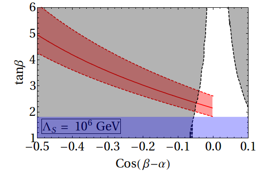
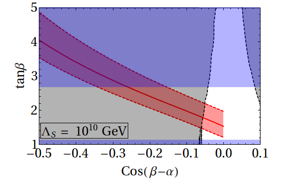
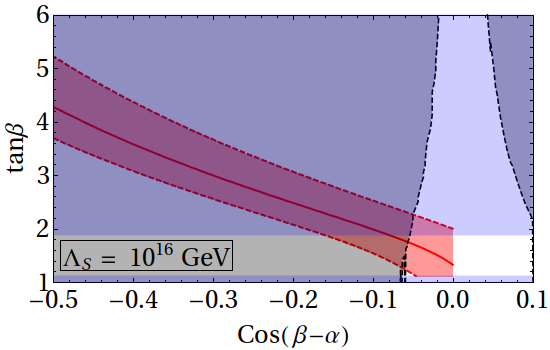
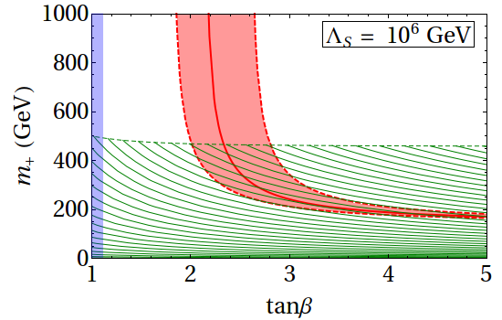
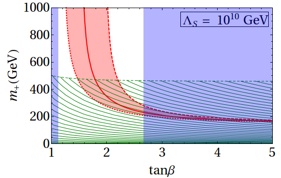
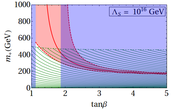
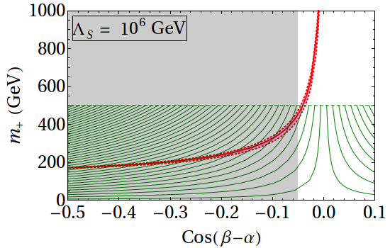
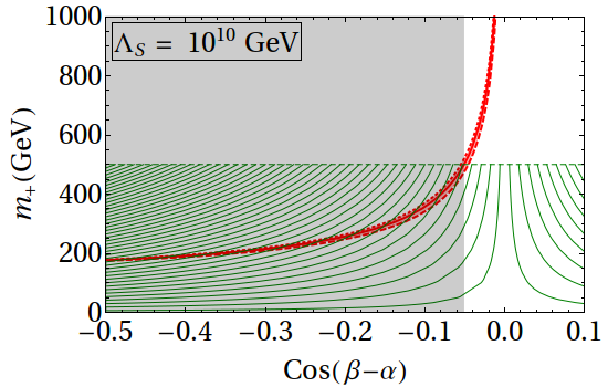
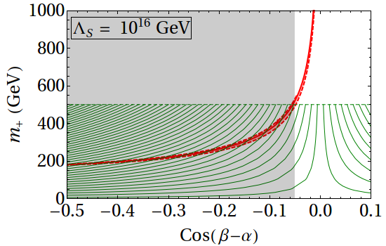
Figure 3: Solution curves in different planes for different choices of $\Lambda_{S}$. The widths of the solution regions (in red) arise from $2\sigma$ experimental uncertainties in $m_{t}$ and $m_{h}$. The regions disallowed from absolute stability (from $M_{Z}$ all the way to $\Lambda_{S}$) have been shaded in blue, while the hatched regions are disfavored from BR($b\to s\gamma$) at 95% C.L. The shaded regions in gray are ruled out from the LHC Higgs data.

4 Constraints and uncertainties of the SUSY scale determination

To justify our choices for the EWS values of the quartic couplings and $\tan\beta$ used in Fig. 1, we perform a numerical study of the available parameter space at low energy, provided the quartic couplings have been fixed by the supersymmetric boundary conditions at $\Lambda_{S}$. We display our results in Fig. 3 for three different choices of $\Lambda_{S}$. Considering the fact that sub-TeV nonstandard scalars, for type II 2HDM, are disfavored from flavor data for $\tan\beta<1$ [41, 42], we concentrate in the $\tan\beta>1$ region for possible interesting phenomenology. The allowed parameter region from this analysis, consistent with $m_{h}=125.0\pm 0.6$ GeV and a top pole mass $m_{t}=173\pm 1$ GeV, has been shaded in red. The width of this region comes from the uncertainties in the input parameters $m_{t}$ and $m_{h}$, around the central continuous line corresponding to their central values. The values of $\tan\beta$ disfavored from absolute stability (from $M_{Z}$ to $\Lambda_{S}$) of the scalar potential has been shaded in blue. The hatched region in the middle and bottom panels of Fig. 3 is disfavored at 95% C.L. from BR($b\to s\gamma$) [43]. The gray shaded region in the top panel is forbidden by the Higgs data at 95% C.L. [44]. The gray region in the bottom panel, however, represents a disallowed region using a conservative bound on $\cos(\beta-\alpha)$ from the Higgs data[44]. Some of the interesting features that emerge from Fig. 3 are summarized below.

1. The main feature of Fig. 3, as apparent from the top and middle panels, is that for a large supersymmetric scale, only low $\tan\beta$ values can reproduce the observed Higgs mass. Taking into account the constraints on $\cos(\beta-\alpha)$ and $m_{+}$ along with the requirement of absolute vacuum stability, we find that $1.8\leq\tan\beta\leq 2.8$ for $\Lambda_{S}=10^{6}$ GeV, while $1.2\leq\tan\beta\leq 2.2$ for $\Lambda_{S}=10^{10}$ GeV and $1.1\leq\tan\beta\leq 1.9$ for $\Lambda_{S}=10^{16}$ GeV. These results are in qualitative agreement with those in Refs. [28, 29] in the aspects where the analyses overlap.

2. It is interesting to note that for large $\Lambda_{S}$ we obtain an upper limit on $\tan\beta$ from the requirement of absolute stability, in addition to a lower limit that stability usually offers in a generic 2HDM where the top Yukawa is proportional to $m_{t}/(v\sin\beta)$ [11]. This upper limit, which is rather strong ($\tan\beta\lesssim 2$ for $\Lambda_{S}=10^{16}$ GeV), arises from the requirement of satisfying $\lambda_{3}+\lambda_{4}+\sqrt{\lambda_{1}\lambda_{2}}\geq|\lambda_{5}|$ [5] at all scales, but in our specific embedding of 2HDM in a SUSY backdrop.

3. From the $\cos(\beta-\alpha)$ vs $m_{+}$ plot, we see that we are practically in the decoupling region [7]. In the middle panel we observe that for a given value of $\tan\beta$, any value of $m_{+}\gtrsim 500$ GeV is possible when we take into account the uncertainties in the parameters. As mentioned before, the allowed range of $\tan\beta$ depends on the scale, $\Lambda_{S}$. It is still, nevertheless, possible to have nonstandard scalars below the TeV scale, which is encouraging for the collider experiments.

4. As expected $m_{+}$ and $\cos(\beta-\alpha)$ are strongly correlated irrespective of the SUSY scale. This is easily understood as this mixing comes from the diagonalization of the neutral Higgs mass matrix in the Higgs basis, with offdiagonal elements ${\cal O}(v^{2})$ and a large diagonal entry ${\cal O}(m_{+}^{2})$.

5. As the allowed region in Fig. 3 is confined around $\tan\beta\sim{\cal O}\left(1\right)$ (for $\Lambda_{s}\geq 10^{6}$ GeV), we have to focus on the left-most side of Fig. 4 where we display the decay pattern of the heavier CP even scalar $H$.

Figure 4: Branching ratios of the heavier scalar, $H$ into different decay channels as a function of $\tan\beta$. We have assumed $|\cos(\beta-\alpha)|\approx 0$ so that $H$ does not decay into a pair of gauge bosons.

As we discussed in Section 2, the variation of $\lambda_{2}$ with the scale is more pronounced than that of other quartic couplings, if we start from small boundary values at high energy. Therefore, $\lambda_{2}$ is our best choice to determine $\Lambda_{S}$ as the scale where it reaches its boundary value $(g^{2}+g_{Y}^{2})/4$. However, this evolution is very sensitive to the values of $m_{t}$ and $\tan\beta$ at the EWS, as well as to the initial $\lambda_{2}$ value.

This behavior of $\lambda_{2}$ is shown in Fig. 5, where we plot it for three similar values of $\tan\beta$ and several closely spaced electroweak values of $\lambda_{2}$ consistent with the observed Higgs mass. In fact, this figure is produced with a fixed value of the top quark mass $m_{t}=173$ GeV; however, the intrinsic top mass error of about $1$ GeV can be reproduced by a shift in $\tan\beta$. Given that the main effect of these uncertainties is a change in the top Yukawa coupling, we can translate both uncertainties as $\Delta\tan\beta=\tan\beta(1+\tan^{2}\beta)(\Delta m_{t}/m_{t})$. From here, we obtain that $\Delta m_{t}=1$ GeV corresponds to $\Delta\tan\beta\sim 0.01$ for $\tan\beta=1$ and $\Delta\tan\beta\sim 0.06$ for $\tan\beta=2$. Thus, for the small $\tan\beta$ values required when $\Lambda_{S}\geq 10^{6}$ GeV, the effect of the top mass uncertainty is smaller than the effect of the $\tan\beta$ range considered in Fig. 5, but it grows as $\tan^{3}\beta$ and will be important for larger values of $\tan\beta$.

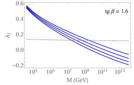
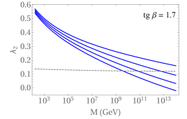
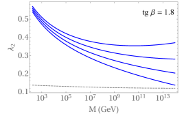
Figure 5: Evolution of $\lambda_{2}$ (low to high scale) as a function of the scale $M$, for different initial values (from bottom to top, $\lambda_{2}=0.54,0.55,0.56,0.57$), as compared with $(g^{2}+g_{Y}^{2})/4$ (dashed line) for different $\tan\beta$ values.

Using Eqs. (3), (4), and (6), we can get an a posteriori explanation for the obtained values of $\lambda_{2}$ and $\tan\beta$ at the EWS. Under the assumptions of sub-TeV nonstandard scalars and very small $\cos(\beta-\alpha)$, Eq. (3) gives $g_{11}v^{2}\simeq m_{h}^{2}$. To a good approximation, we can also write

$$\lambda_{1}(M_{Z})\simeq\lambda_{1}(\Lambda_{S})=\lambda_{2}(\Lambda_{S})=\frac{(g^{2}+g_{Y}^{2})}{4}=-\left\{\lambda_{3}(\Lambda_{S})+\lambda_{4}(\Lambda_{S})\right\}\simeq-\left\{\lambda_{3}(M_{Z})+\lambda_{4}(M_{Z})\right\}\,.$$ (9)

Now, using Eq. (2a), we obtain

$$m_{h}^{2}=M_{Z}^{2}\cos^{2}(2\beta)+\Delta\lambda_{2}v^{2}~{}\frac{\tan^{4}\beta}{\left(1+\tan^{2}\beta\right)^{2}}=M_{Z}^{2}\left(\frac{\tan^{2}\beta-1}{\tan^{2}\beta+1}\right)^{2}+\Delta\lambda_{2}v^{2}~{}\left(\frac{\tan^{2}\beta}{1+\tan^{2}\beta}\right)^{2}\,,$$ (10)

where, $\Delta\lambda_{2}=\lambda_{2}(M_{Z})-\lambda_{2}(\Lambda_{S})$. Eq. (10) can easily be recognized as the usual expression for the radiatively improved Higgs mass in the MSSM. This implies that the mass of the observed Higgs boson is essentially determined by the RG evolution of $\lambda_{2}$ and the value of $\tan\beta$. For a fixed value of $\tan\beta$, the low energy value of $\lambda_{2}$ is uniquely determined by $m_{h}$. The larger the gap between $\Lambda_{S}$ and $M_{Z}$, the more room $\lambda_{2}$ gets to grow under RG evolution, thereby requiring a smaller $\tan\beta$ to reproduce the observed Higgs mass.

To put our results into perspective, let us assume that all the nonstandard scalar masses have been determined with an accuracy of 1 GeV viz., $m_{H}=(503\pm 1)$ GeV, $m_{A}=(491\pm 1)$ GeV, $m_{+}=(496\pm 1)$ GeV, and we have settled at $\cos(\beta-\alpha)=-0.05$ and $\tan\beta=1.7$. These values would correspond to a supersymmetric scale of $\Lambda_{S}\sim 10^{10}$ GeV. However, it should be noted that such an estimate of the SUSY scale is very sensitive to the precise values of the input parameters, especially $\tan\beta$, and as shown in Fig. 5; we would need to determine $\tan\beta$ at a few percent level to fix $\Lambda_{S}$ precisely. This ambiguity in the determination of the SUSY scale may partly be attributed to a common solution region for $\Lambda_{S}$ in the range of $10^{6}$-$10^{16}$ GeV, as apparent from Fig. 3 (see point (a) of Sec. 4 also). On the other hand, if $\tan\beta$ turns out to be close to $2.2$ (say), then one can, for example, make a definitive conclusion that $\Lambda_{S}\leq 10^{10}$ GeV. Such a precise measurement of $\tan\beta$ would, perhaps, require us to wait for the future linear colliders. Nonetheless, the analysis presented in this paper is good enough to provide an initial hint for the location of the scale where SUSY is expected to appear.

5 Conclusions

Our intention in this work was to address the question we posed in the title as directly as possible. To this end, we explored an effective 2HDM arising from a more fundamental theory at a high scale, $\Lambda_{S}$, which fixes the parameters of the Higgs potential. In particular, we have focused on the high-scale MSSM as an example, where the Higgs quartic couplings are determined by the supersymmetry breaking $D$-terms as functions of the gauge couplings. We have found that very high-scale MSSM scenarios are still compatible with the observed Higgs mass for $\tan\beta\sim{\cal O}\left(1\right)$. Though our approach and emphasis is somewhat different, we agree with the general conclusions of the existing analyses studying effective 2HDMs stemming from high scale SUSY wherever we overlap.

We emphasize that our methodology is quite general and can be applied not only to SUSY but to a wide variety of UV scenarios in which all the quartic couplings of the 2HDM potential of Eq. (1) are fixed at a high scale, $\Lambda_{S}$. For instance, we could have started with the assumption that all the quartic couplings vanish at $\Lambda_{S}$. For this particular scenario, we find that the requirement of $m_{h}\approx 125$ GeV, $v=246$ GeV and $|\cos(\beta-\alpha)|\sim 0$ and the absolute stability of the potential up to $\Lambda_{S}$ favors a region of large $\tan\beta\sim 50$. In this region, the evolution of the quartic couplings makes the charged scalar rather light, $m_{+}\approx 180$ GeV, which is ruled out from the measurement of BR($b\to s\gamma$). This particular scenario is, therefore, disfavored by the experimental data.

In the context of the supersymmetry, our analysis shows how possible (future) measurements of the nonstandard scalar masses, $\tan\beta$ and $\cos(\beta-\alpha)$ can fix the $\lambda_{1,2,3,4}$ couplings of the 2HDM potential, neglecting $\lambda_{5,6,7}$, as is natural in the MSSM. Using the 2HDM RGE we find that $\lambda_{1}$ and $-(\lambda_{3}+\lambda_{4})$ should stay close to their boundary value, $(g^{2}+g_{Y}^{2})/4$, all the way from $\Lambda_{S}$ to $M_{Z}$, while $\lambda_{2}$ can grow significantly during RG running due to the large top Yukawa coupling. This opens up the possibility of determining the supersymmetric scale, $\Lambda_{S}$, from the RG evolution of $\lambda_{2}$ as the scale where $\lambda_{2}$ reaches its boundary value, $(g^{2}+g_{Y}^{2})/4$. However, this strategy crucially depends on whether $\tan\beta$ can be determined with a percent level precision in order to make a reasonable prediction for the MSSM scale; a linear collider would be essential to make further inroads.

References

- [1] CMS collaboration, S. Chatrchyan et al., Observation of a new boson at a mass of 125 GeV with the CMS experiment at the LHC, Phys. Lett. B716 (2012) 30–61, [1207.7235].
- [2] ATLAS collaboration, G. Aad et al., Observation of a new particle in the search for the Standard Model Higgs boson with the ATLAS detector at the LHC, Phys. Lett. B716 (2012) 1–29, [1207.7214].
- [3] CMS collaboration, V. Khachatryan et al., Precise determination of the mass of the Higgs boson and tests of compatibility of its couplings with the standard model predictions using proton collisions at 7 and 8 TeV, Eur. Phys. J. C75 (2015) 212, [1412.8662].
- [4] ATLAS, CMS collaboration, G. Aad et al., Measurements of the Higgs boson production and decay rates and constraints on its couplings from a combined ATLAS and CMS analysis of the LHC pp collision data at and 8 TeV, JHEP 08 (2016) 045, [1606.02266].
- [5] G. C. Branco, P. M. Ferreira, L. Lavoura, M. N. Rebelo, M. Sher and J. P. Silva, Theory and phenomenology of two-Higgs-doublet models, Phys. Rept. 516 (2012) 1–102, [1106.0034].
- [6] G. Bhattacharyya and D. Das, Scalar sector of two-Higgs-doublet models: A minireview, Pramana 87 (2016) 40, [1507.06424].
- [7] J. F. Gunion and H. E. Haber, The CP conserving two Higgs doublet model: The Approach to the decoupling limit, Phys. Rev. D67 (2003) 075019, [hep-ph/0207010].
- [8] M. Carena, I. Low, N. R. Shah and C. E. M. Wagner, Impersonating the Standard Model Higgs Boson: Alignment without Decoupling, JHEP 04 (2014) 015, [1310.2248].
- [9] P. S. Bhupal Dev and A. Pilaftsis, Maximally Symmetric Two Higgs Doublet Model with Natural Standard Model Alignment, JHEP 12 (2014) 024, [1408.3405].
- [10] G. Bhattacharyya and D. Das, Nondecoupling of charged scalars in Higgs decay to two photons and symmetries of the scalar potential, Phys. Rev. D91 (2015) 015005, [1408.6133].
- [11] D. Das and I. Saha, Search for a stable alignment limit in two-Higgs-doublet models, Phys. Rev. D91 (2015) 095024, [1503.02135].
- [12] H. P. Nilles, Supersymmetry, Supergravity and Particle Physics, Phys. Rept. 110 (1984) 1–162.
- [13] H. E. Haber and G. L. Kane, The Search for Supersymmetry: Probing Physics Beyond the Standard Model, Phys. Rept. 117 (1985) 75–263.
- [14] J. D. Lykken, Introduction to supersymmetry, in Fields, strings and duality. Proceedings, Summer School, Theoretical Advanced Study Institute in Elementary Particle Physics, TASI’96, Boulder, USA, June 2-28, 1996, pp. 85–153, 1996. hep-th/9612114.
- [15] S. P. Martin, A Supersymmetry primer, hep-ph/9709356.
- [16] M. Drees, R. Godbole and P. Roy, Theory and phenomenology of sparticles: An account of four-dimensional N=1 supersymmetry in high energy physics. 2004.
- [17] H. Baer and X. Tata, Weak scale supersymmetry: From superfields to scattering events. Cambridge University Press, 2006.
- [18] G. F. Giudice and A. Strumia, Probing High-Scale and Split Supersymmetry with Higgs Mass Measurements, Nucl. Phys. B858 (2012) 63–83, [1108.6077].
- [19] A. Arvanitaki, N. Craig, S. Dimopoulos and G. Villadoro, Mini-Split, JHEP 02 (2013) 126, [1210.0555].
- [20] E. Bagnaschi, G. F. Giudice, P. Slavich and A. Strumia, Higgs Mass and Unnatural Supersymmetry, JHEP 09 (2014) 092, [1407.4081].
- [21] J. Pardo Vega and G. Villadoro, SusyHD: Higgs mass Determination in Supersymmetry, JHEP 07 (2015) 159, [1504.05200].
- [22] G. Isidori and A. Pattori, On the tuning in the plane: Standard Model criticality vs. High-scale SUSY, 1710.11060.
- [23] M. Carena, J. Ellis, J. S. Lee, A. Pilaftsis and C. E. M. Wagner, CP Violation in Heavy MSSM Higgs Scenarios, JHEP 02 (2016) 123, [1512.00437].
- [24] P. Athron, J.-h. Park, T. Steudtner, D. Stockinger and A. Voigt, Precise Higgs mass calculations in (non-)minimal supersymmetry at both high and low scales, JHEP 01 (2017) 079, [1609.00371].
- [25] F. Staub and W. Porod, Improved predictions for intermediate and heavy Supersymmetry in the MSSM and beyond, Eur. Phys. J. C77 (2017) 338, [1703.03267].
- [26] H. E. Haber, S. Heinemeyer and T. Stefaniak, The Impact of Two-Loop Effects on the Scenario of MSSM Higgs Alignment without Decoupling, Eur. Phys. J. C77 (2017) 742, [1708.04416].
- [27] G. Chalons, A. Djouadi and J. Quevillon, The neutral Higgs self-couplings in the (h)MSSM, 1709.02332.
- [28] G. Lee and C. E. M. Wagner, Higgs bosons in heavy supersymmetry with an intermediate mA, Phys. Rev. D92 (2015) 075032, [1508.00576].
- [29] E. Bagnaschi, F. Brummer, W. Buchmuller, A. Voigt and G. Weiglein, Vacuum stability and supersymmetry at high scales with two Higgs doublets, JHEP 03 (2016) 158, [1512.07761].
- [30] S. A. R. Ellis and J. D. Wells, High-scale supersymmetry, the Higgs boson mass, and gauge unification, Phys. Rev. D96 (2017) 055024, [1706.00013].
- [31] J. D. Wells and Z. Zhang, Effective field theory approach to trans-TeV supersymmetry: covariant matching, Yukawa unification and Higgs couplings, 1711.04774.
- [32] M. E. Machacek and M. T. Vaughn, Two Loop Renormalization Group Equations in a General Quantum Field Theory. 2. Yukawa Couplings, Nucl. Phys. B236 (1984) 221–232.
- [33] M. E. Machacek and M. T. Vaughn, Two Loop Renormalization Group Equations in a General Quantum Field Theory. 1. Wave Function Renormalization, Nucl. Phys. B222 (1983) 83–103.
- [34] M. E. Machacek and M. T. Vaughn, Two Loop Renormalization Group Equations in a General Quantum Field Theory. 3. Scalar Quartic Couplings, Nucl. Phys. B249 (1985) 70–92.
- [35] F. Staub, SARAH 4 : A tool for (not only SUSY) model builders, Comput. Phys. Commun. 185 (2014) 1773–1790, [1309.7223].
- [36] G. Bhattacharyya, D. Das, P. B. Pal and M. N. Rebelo, Scalar sector properties of two-Higgs-doublet models with a global U(1) symmetry, JHEP 10 (2013) 081, [1308.4297].
- [37] J. Bernon, J. F. Gunion, H. E. Haber, Y. Jiang and S. Kraml, Scrutinizing the alignment limit in two-Higgs-doublet models: mh=125 GeV, Phys. Rev. D92 (2015) 075004, [1507.00933].
- [38] D. J. H. Chung, L. L. Everett, G. L. Kane, S. F. King, J. D. Lykken and L.-T. Wang, The Soft supersymmetry breaking Lagrangian: Theory and applications, Phys. Rept. 407 (2005) 1–203, [hep-ph/0312378].
- [39] H. E. Haber and R. Hempfling, The Renormalization group improved Higgs sector of the minimal supersymmetric model, Phys. Rev. D48 (1993) 4280–4309, [hep-ph/9307201].
- [40] J. Braathen, M. D. Goodsell, M. E. Krauss, T. Opferkuch and F. Staub, Match before you run: N is better than N-1, 1711.08460.
- [41] O. Deschamps, S. Descotes-Genon, S. Monteil, V. Niess, S. T’Jampens and V. Tisserand, The Two Higgs Doublet of Type II facing flavour physics data, Phys. Rev. D82 (2010) 073012, [0907.5135].
- [42] D. Das, New limits on tan for 2HDMs with Z2 symmetry, Int. J. Mod. Phys. A30 (2015) 1550158, [1501.02610].
- [43] M. Misiak and M. Steinhauser, Weak radiative decays of the B meson and bounds on in the Two-Higgs-Doublet Model, Eur. Phys. J. C77 (2017) 201, [1702.04571].
- [44] J. Bernon, B. Dumont and S. Kraml, Status of Higgs couplings after run 1 of the LHC, Phys. Rev. D90 (2014) 071301, [1409.1588].
- [45] D. Chowdhury and O. Eberhardt, Update of Global Two-Higgs-Doublet Model Fits, 1711.02095.