Statistical analysis of random trajectories of vibrated disks:
towards a macroscopic realization of Brownian motion

Abstract

We propose a macroscopic realization of planar Brownian motion by vertically vibrated disks. We perform a systematic statistical analysis of many random trajectories of individual disks. The distribution of increments is shown to be almost Gaussian, with slight deviations at large increments caused by inter-disk collisions. The velocity auto-correlation function takes both positive and negative values at short lag times but rapidly vanishes. We compare the empirical and theoretical distributions of time averaged mean square displacements and discuss distinctions between its mean and mode. These well-controlled experimental data can serve for validating statistical tools developed for the analysis of single-particle trajectories in microbiology.

I Introduction

One of the first reports of Brownian motion is attributed to the Scottish botanist Robert Brown who observed in a microscope a continuous jittery motion of minute particles ejected from the Clarkia pollen grains suspended in water Brown1828 . Since a more systematic study by Jean Perrin Perrin1908 ; Perrin1909 , the abundant experimental evidence of Brownian motion of microscopic particles has been established Frey05 ; Grebenkov07 ; Sackmann10 ; Brauchle . The mathematical origin of this abundance lies in the central limit theorem which implies a universal probabilistic description of motion at mesoscopic time and length scales, regardless microscopic dynamics. In turn, experimental observations of Brownian motion in the macroscopic world are rarer. In fact, it is quite difficult to design an experiment with macroscopic objects that would result in Brownian trajectories. On one hand, the motion is strongly influenced by inertial effects, resulting in ballistic segments of the trajectory at the macroscopic scale (e.g., the motion of balls in a billiard). On the other hand, the number of interacting objects in a macroscopic system is much smaller than the number of water molecules involved in the motion of a microscopic particle, whereas the separation between the time scale of an elementary displacement and the duration of the measurement is not large enough. As a consequence, the motion of macroscopic objects is not enough randomized by their collisions. In particular, the dynamics of granular matter is typically far from Brownian motion Jaeger96 ; Choi04 ; Grebenkov08 ; Chen09 ; Scalliet15 . For instance, there is a rather narrow range of packing fractions, for which the motion of spherical beads is fluid-like: in the low density regime, collisions between beads are rare while the mean free path is long so that too large experimental setups would be needed to observe a Brownian trajectory; in the high density regime, inter-bead collisions are often but collective modes of motion (e.g., crystallization or jamming) become dominant.

From the practical point of view, a well-controlled experimental realization of a macroscopic diffusive motion with an excellent statistics of long trajectories can serve as a benchmark for testing various statistical tools developed for the analysis of single particle trajectories (see Qian91 ; Arcizet08 ; Metzler09 ; Michalet10 ; Berglund10 ; Michalet12 ; Vestergaard14 ; Gal13 ; Kepten15 ; Magdziarz11 ; Lanoiselee16 ; Lanoiselee17 and references therein). In fact, it is essential to disentangle finite time average and finite sampling effects when performing single probe experiments in biology (e.g., the intracellular transport or the motion of proteins on cell membranes). While statistical tools are commonly tested on simulated trajectories, a macroscopic realization of diffusive motions can present a rare opportunity to confront simulations and theoretical results to an experimental situation with true experimental noise, uncertainties, resolution issues, etc.

In this paper, we report an experimental observation of the diffusive motion realized by macroscopic disks of 4 mm diameter on a vertically vibrating plate (see Sec. II). Vibrations pump in the system the kinetic energy that substitutes thermal energy that drives the motion in a microscopic system. We undertake a systematic statistical analysis of the acquired trajectories of individual disks (Sec. III). In particular, we analyze the distribution of one-step displacements, the ergodicity, the velocity auto-correlation function, and the distribution of time averaged mean square displacements (TAMSD). This analysis shows that the macroscopic motion of disks exhibits small deviations from Brownian motion at short times but approaches it at longer times.

II Experimental setup

The experimental system, made of vibrated disks, has been described in details previously Deseigne12 . We recall here the key ingredients of the set-up. Experiments with shaken granular particles are notoriously susceptible to systematic deviations from pure vertical vibration and special care must be taken to avoid them. First, to ensure the rigidity of the tray supporting the particles, we use a $110$ mm thick truncated cone of expanded polystyrene sandwiched between two nylon disks. The top disk (diameter $425$ mm) is covered by a glass plate on which lay the particles. The bottom one (diameter $100$ mm) is mounted on the slider of a stiff square air-bearing (C40-03100-100254, IBSPE), which provides virtually friction-free vertical motion and submicron amplitude residual horizontal motion. The vertical alignment is controlled by set screws. The vibration is produced with an electromagnetic servo-controlled shaker (V455/6-PA1000L,LDS), the accelerometer for the control being fixed at the bottom of the top vibrating disk, embedded in the expanded polystyren. A $400$ mm long brass rod couples the air-bearing slider and the shaker. It is flexible enough to compensate for the alignment mismatch, but stiff enough to ensure mechanical coupling. The shaker rests on a thick wooden plate ballasted with $460$ kg of lead bricks and isolated from the ground by rubber mats (MUSTshock 100x100xEP5, Musthane). We have measured the mechanical response of the whole setup and found no resonances in the window $70-130$ Hz. We use a sinusoidal vibration of frequency $f=95$ Hz and set the relative acceleration to gravity $\Gamma=a(2\pi f)^{2}/g=2.4$, where the vibration amplitude $a$ at a peak acceleration is $100~{}\mu$m. Using a triaxial accelerometer (356B18, PCB Electronics), we checked that the horizontal to vertical ratio is lower than $10^{-2}$ and that the spatial homogeneity of the vibration is better than $1\%$.

The particles are micro-machined copper-beryllium disks (diameter $d=4\pm 0.03$ mm). The contact with the vibrating plate is that of an extruded cylinder, resulting in a total height $h=2.0$ mm. They are sandwiched between two thick glass plates separated by a gap $H=2.4$ mm and laterally confined in an arena of diameter $320$ mm. A CCD camera with a spatial resolution of 1728 x 1728 pixels and standard tracking software is used to capture the motion of the particles at a frame rate of $25$ Hz. In a typical experiment, the motion of the disks is recorded during $600$ seconds, producing $15~{}000$ images. The resolution on the position $\vec{r}$ of the particles is better than $0.05$ particle diameter (i.e., $0.2$ mm).

In the following, particle trajectories are tracked within a circular region of interest (ROI) of diameter $50d=200$ mm far from the border of the arena, where the long-time averaged density field is homogeneous. The average packing fractions $\phi$ measured inside the ROI ranges from $0.3$ to $0.64$, and the total number of particles ranges from $1000$ to $2500$. As the onset of spatial order typically takes place at $\phi_{\dagger}\simeq 0.71$, we always deal with a liquid state.

III Statistical analysis

We performed a systematic statistical analysis of the acquired random trajectories. Examples of such trajectories are shown in Fig. 1.

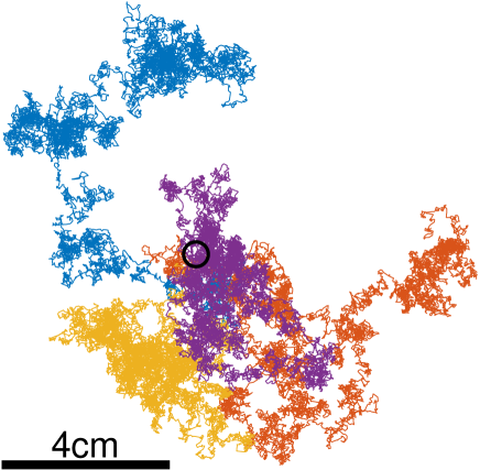
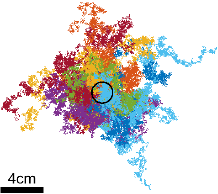
Figure 1: (Color online) (Top) Example of random trajectories of 4 disks that were originally located close to each other (inside the black circle) and then diffused during 600 seconds (i.e., 15 000 points in each trajectory). (Bottom) Example of random trajectories of 34 disks that were originally located close to each other and then diffused during 464.6 seconds (i.e., 11 615 points in each trajectory).

III.1 Data description

We analyzed 14 samples with different surface packing fractions $\phi$, ranging between $0.298$ and $0.637$ (Table 1). The time step (i.e., the duration of one displacement) is fixed by the acquisition frequency: $\delta=1/25~{}\textrm{Hz}=0.04$ s. The positions are measured in units of the disk diameter, $d=4$ mm. To avoid boundary effects, only the disks within the ROI were used for the analysis. In particular, a trajectory is terminated when the disk leaves the ROI, and a new trajectory is initiated when a disk enters the ROI. As a consequence, the acquired trajectories have very different lengths varying from $1$ to $15\,000$. To improve the statistical accuracy of our results, we discarded all the trajectories whose length was shorter than $1000$. The disks exhibited multiple mutual collisions during the experiments. Although the collective motion of these disks might be studied as the dynamics of interacting particles in a large phase space, we look at this problem from the single-particle point of view and treat each disk as a single particle interacting with its complex dynamic environment. This view is typical for single-particle tracking experiments in microbiology when one can record only the motion of a labeled (e.g., fluorescent) particle, whereas the dynamics of all other constitutes of the cytoplasm remains inaccessible.

sample	$\phi$	std/$d$	$D$ (in mm2/s)
1	0.298	0.0956	1.83
2	0.324	0.0938	1.76
3	0.350	0.0932	1.74
4	0.376	0.1048	2.20
5	0.402	0.1025	2.10
6	0.428	0.1107	2.45
7	0.454	0.1052	2.21
8	0.480	0.1005	2.02
9	0.507	0.0978	1.91
10	0.533	0.0950	1.81
11	0.559	0.0926	1.71
12	0.585	0.0942	1.78
13	0.611	0.0936	1.75
14	0.637	0.0895	1.60

Table 1: Summary of experimental data: the sample index, the surface fraction $\phi$, the standard deviation of one-step one-dimensional increments (in units of the disk diameter $d=4$ mm), and the corresponding diffusion coefficient: $D={\rm std}^{2}/(2\delta)$, with $\delta=0.04$ s. For comparison the maximal disk packing fraction, corresponding to the close-packed hexagonal lattice, is $\pi/(2\sqrt{3})\simeq 0.9069$; and the crystallization transition for equilibrium hard disks takes place at $\phi_{\dagger}\simeq 0.71$.

III.2 Distribution of increments

We start by verifying whether the one-step increments obey a Gaussian distribution. For each sample, we collected the one-step increments along $X$ and $Y$ axes for each trajectory in the sample and constructed their histogram. Having checked for the isotropy of the statistics, we focus on one-dimensional increments and merge increments along $X$ and $Y$ coordinates in order to get a representative statistics even for large increments. Figure 2(a) shows these histograms (presented in the form of probability densities at the semilogarithmic scale) for 14 samples. These densities are close to each other and exhibit a parabolic shape reminiscent of a Gaussian distribution. The standard deviations of one-step increments are summarized in Table 1. These values are also close to each other and show no systematic dependence on the packing fraction. At first sight, there is no systematic variation of probability densities with the packing fraction. This suggests that the randomness of motion essentially comes from the rotational symmetry of the disk, which undergoes a displacement in a random direction after each kick by the vibrating plate. Note that the frequency of plate vibrations is 4 times higher than the acquisition frequency meaning that each displacement results from 4 random kicks.

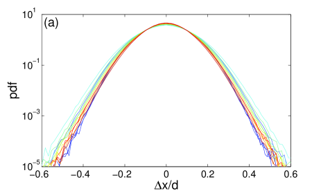
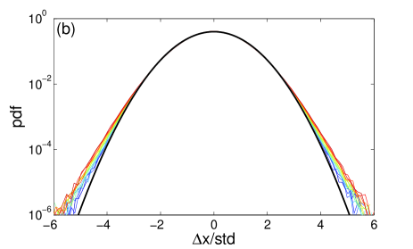
Figure 2: (Color online) (a) The empirical distributions of one-step one-dimensional increments for 14 samples (in units of the disk diameter, $d=4$ mm). (b) The empirical distributions of rescaled one-step increments for 14 samples. Thick black curve shows the standard Gaussian density $e^{-x^{2}/2}/\sqrt{2\pi}$. Color of thin curves changes from dark blue for the lowest packing fraction $\phi$ to dark red for the highest one.

Despite their delicate machining, the precise contact of the disks with the vibrating plate is influenced by minor asperities, which differ from disk to disk but also depend on the location of the disks on the vibrating plate. In order to reduce these factors of diversity, we rescale the one-step increments from one trajectory by the empirical standard deviation of these increments. Such a rescaling partly levels off eventual heterogeneities between trajectories. Once calculated, the rescaled increments along $X$ and $Y$ coordinates are merged from different trajectories in each sample. The obtained distributions are presented in Fig. 2(b). One can see that the distributions for all 14 samples almost collapse and remain close to the standard Gaussian density $\exp(-x^{2}/2)/\sqrt{2\pi}$. However, now that heterogeneities between trajectories have been levelled off by the rescaling, one distinguishes small but statistically significant deviations for large increments. These deviations progressively increase with the packing fraction, and can therefore be attributed to disk-disk collisions.

III.3 Ergodicity hypothesis

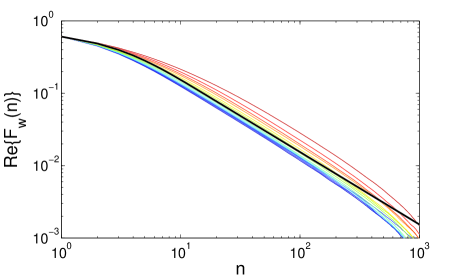
Figure 3: (Color online) The real part of the ergodicity estimator, ${\rm Re}\{\hat{F}_{\omega}(n)\}$ (with $\omega=1/\sigma$), averaged over trajectories in each of 14 samples (thin lines). Color of thin curves changes from dark blue for the lowest packing fraction $\phi$ to dark red for the highest one. Thick black line shows the mean value of this estimator for Brownian motion.

We analyze whether the system of vibrated disks can be considered as being at equilibrium. In practice, we test the ergodicity hypothesis which is a necessary but not sufficient condition for equilibrium. The ergodicity hypothesis claims that the ensemble average over many particles is equal to the time average over an (infinitely) long trajectory of one particle. Under the stationarity hypothesis of the motion, we employ the ergodicity estimator $\hat{F}_{\omega}(n)$ Magdziarz11 ; Lanoiselee16

$$\hat{F}_{\omega}(n)\equiv\frac{1}{n}\sum\limits_{k=1}^{n}\hat{E}_{\omega}(k),$$ (1)

with

$$\hat{E}_{\omega}(n) \equiv \frac{1}{N-n+1}\sum\limits_{k=0}^{N-n}e^{i\omega[X(k+n)-X(k)]}$$ (2)

$$- \frac{1}{N(N+1)}\left|\sum\limits_{k=0}^{N}e^{i\omega[X(k)-X(0)]}\right|^{2}+\frac{1}{N}.$$

where $X(k)$ are successive $X$ coordinates of the points $\bm{x}_{k}$ along a given trajectory of length $N$ (the same analysis was performed for the $Y$ coordinate, not shown). The first term can be interpreted as the time averaged characteristic function of the increment $X(k+n)-X(k)$ at lag time $n$, while the second term ensures that the estimator is strictly $0$ for a constant process $X(n)=X_{0}$ (in addition, the mean estimator is strictly $0$ for a process with independent $X(n)$). For Brownian motion, the mean value of the estimator is Lanoiselee16 :

$${\mathbb{E}}\{\hat{F}_{\omega}(n)\}=q\frac{1-q^{n}}{n(1-q)}+O(1/N),$$ (3)

where $q=e^{-\omega^{2}\sigma^{2}/2}$ and $\sigma^{2}$ is the variance of one-step increments. To eliminate the effect of length scale, we set $\omega=1/\sigma$ that is equivalent to rescaling the trajectory by the standard deviation $\sigma$.

Figure 3 shows the real part of the ergodicity estimator averaged over all the trajectories in each of 14 samples. For small $n$, higher the packing fraction, slower the decrease of the estimator with $n$. However, for large $n$ the $1/n$ scaling predicted in the case of the Brownian motion is recovered and we can safely formulate the hypothesis that ergodicity is satisfied.

III.4 Velocity auto-correlations

We also study the velocity auto-correlations function (VACF) which is defined as

$$C(t)=\langle\bm{v}(t)\cdot\bm{v}(0)\rangle\,,$$ (4)

where $\bm{v}(t)$ is the velocity at time $t$, and $\langle\cdots\rangle$ is the ensemble average. In the experimental setting, the positions are recorded with the time step $\delta=0.04$ s, so that $t=n\delta$, and the velocity is proportional to the one-step increment: $\bm{v}(n\delta)=(\bm{x}_{n+1}-\bm{x}_{n})/\delta$, with $\bm{x}_{n}=\bm{x}(n\delta)$. To improve statistics, we combine the time average along the trajectory of each disk and the ensemble average over many trajectories:

$$C(n\delta)=\frac{1}{M\delta^{2}}\sum\limits_{m=1}^{M}\frac{1}{N_{m}-n-1}\sum\limits_{k=1}^{N_{m}-n-1}\bigl{(}\Delta\bm{x}_{n+k}^{(m)}\cdot\Delta\bm{x}_{k}^{(m)}\bigr{)},$$ (5)

where $\Delta\bm{x}_{n}^{(m)}=\bm{x}^{(m)}_{n+1}-\bm{x}^{(m)}_{n}$ is the $n$-th one-step increment of the $m$-th disk, $M$ is the number of disks in a sample, and $N_{m}$ is the length of the $m$-th trajectory.

Figure 4 shows the normalized VACF, $C(n\delta)/C(0)$, which varies between $-1$ and $1$, as a function of the lag time $n\delta$. For all considered samples, the VACF rapidly decreases with time and becomes close to zero for $n\gtrsim 10$. By construction, the normalized VACF is equal to $1$ at $n=0$. Positive auto-correlations at lag time $n=1$ can potentially be attributed to inertial effects. The negative auto-correlations observed for $n>1$ take their root in an excess of reverse bouncing of the disks when they successively hit the trail, but not only. Since they become more pronounced when the packing fraction increases, they should also come from collisions. In all cases, although the successive increments exhibit small but noticeable correlations, they drop very rapidly as the lag time increases. We recall that the normalized VACF for a discrete-time Brownian motion (a random walk) is $1$ for $n=0$ and $0$ otherwise. Strictly speaking, the disk trajectories acquired at time step $\delta=0.04$ s are therefore not Brownian but remain close to Brownian ones.

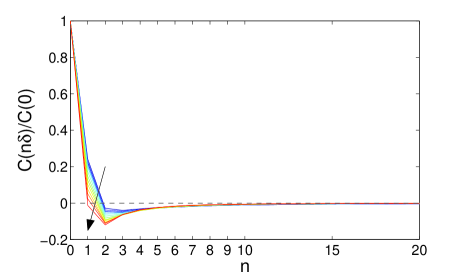
Figure 4: The normalized VACF, $C(n\delta)/C(0)$, as a function of the lag time $n\delta$, for 14 samples. Color changes from dark blue for the lowest packing fraction $\phi$ to dark red for the highest one. This change is also indicated by an arrow.

III.5 Estimation of diffusion coefficient

Now we focus on the time averaged mean square displacement, which is the most common statistical tool to probe diffusive properties of single-particle trajectories Gal13 . The TAMSD with the lag time $n$ over a trajectory of length $N$ is defined as

$$\chi_{n,N}=\frac{1}{N-n}\sum\limits_{k=1}^{N-n}\|\bm{x}_{k+n}-\bm{x}_{k}\|^{2}.$$ (6)

If $\bm{x}_{k}$ are positions of planar Brownian motion with diffusion coefficient $D$, then the ergodicity of this process implies that

$$\chi_{n,N}\xrightarrow[N\to\infty]{}4Dt=4Dn\delta,$$ (7)

whereas the variance of $\chi_{n,N}$ vanishes as $N\to\infty$ Qian91 ; Grebenkov11 . In other words, the TAMSD allows one to estimate the diffusion coefficient $D$ from a single random trajectory, and longer the trajectory, better the estimation.

For a fixed $N$, the smallest variance (and thus the best estimation) corresponds to $n=1$, in which case $\chi_{1,N}$ is the estimator of the variance of increments. This estimator is known to be optimal for the case of Brownian motion, i.e., it is the best possible way to estimate the diffusion coefficient Cramer ; Grebenkov11 ; Grebenkov13 . In practice, however, even if the studied particle is supposed to undergo Brownian motion, the acquired trajectory can be altered by various “measurement noises” such as localization error, electronic noise, drift or vibrations of the sample, post-processing errors, etc. When some of these noises are anticipated, the estimator can be adapted to provide the (nearly) optimal estimation Michalet10 ; Berglund10 ; Michalet12 ; Grebenkov13 ; Vestergaard14 . However, the Brownian character of the studied but yet unknown process is not granted and has to be checked from the analysis of the TAMSD. In this situation, the rule of thumb consists in plotting the TAMSD versus the lag time $n$ to first check the linear dependence and then to estimate the diffusion coefficient from the slope of the linear plot. Given the randomness of the TAMSD, this procedure can bring biases and additional statistical errors. Moreover, since fluctuations of the TAMSD grow with $n$ (see Qian91 ; Grebenkov11 ), the fit is often limited to small $n$. Figure 5 illustrates large fluctuations of the TAMSD estimator around the ensemble averaged TAMSD which exhibits a linear growth with $n$. As a consequence, an accurate estimation of the diffusion coefficient from a single trajectory is only possible over a narrow range of small lag times $n$. Note that the diffusion coefficient fitted by the ensemble average, $1.47$ mm²/s, is smaller than that estimated from the standard deviation of one-step increments, $1.83$ mm²/s (see Table 1). This discrepancy can be caused by eventual noises (that would affect the standard deviation of one-step increments) and auto-correlations (that would affect the TAMSD).

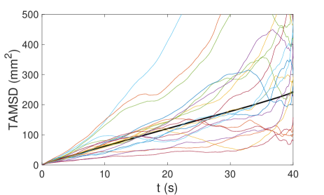
Figure 5: The time averaged MSD, $\chi_{n,N}$, as a function of the lag time $t=n\delta$ (with $n$ varying from $1$ to $1000$), for 10 trajectories of length $N=1001$ from the sample 1 with the lowest packing fraction. Black thick line shows the ensemble average of TAMSD over 12444 trajectories of length $N=1001$ in this sample. The fitted diffusion coefficient from this line is $1.47$ mm²/s.

III.6 Distribution of TAMSD

One of the significant advantages of single-particle tracking is the possibility to infer information from single events, without ensemble averages. This is particularly important in microbiology because many events in a cell life are triggered by a small number of molecules. Even when many particles are tracked simultaneously, they explore different spatial regions of the cell and experience different interactions with the intracellular environment. If infered properly, such heterogeneities may bring a much more detailed information about the cell than an ensemble average. The estimation of the diffusion coefficient from each single trajectory naturally leads to their distribution Duits09 ; Otten12 ; Nandi12 . However, it is important to stress that the experimentally obtained distributions include two sources of randomness: (i) the biological variability and (ii) the intrinsic randomness of the TAMSD estimator obtained from a single finite length trajectory. As a consequence, a proper biological interpretation of such distributions requires to disentangle two sources and, ideally, to remove the second one. This correction needs the knowledge of the distribution of the TAMSD estimator.

The distribution of TAMSD in the biological context was first studied via numerical simulations by Saxton Saxton93 ; Saxton97 . A more general theoretical analysis of TAMSD for Gaussian processes was later performed in Refs. Grebenkov11 ; Andreanov12 ; Grebenkov13 ; Sikora17 . We compute the distribution numerically via the inverse Fourier transform of the characteristic function of TAMSD for which the exact matrix formula was provided in Ref. Grebenkov11 . This computation was shown to be fast and very accurate.

The theoretical distribution of TAMSD for Brownian motion can be compared to the empirical distribution of TAMSD obtained from the trajectories of disks. On one hand, this comparison allows one to check to which extent the acquired trajectories are close to Brownian motion. On the other hand, one can investigate in a well-controlled way the applicability of the theoretical distribution to experimental data.

Figure 6(a) shows the empirical distribution of TAMSD with the lag time $n=1$ obtained by splitting each trajectory into fragments of length $N=100$. This artificial splitting is performed to be closer to the common situation in biological applications, when the acquired trajectories are rather short. Moreover, such splitting significantly improves the statistics of the TAMSD. We compare the probability density functions of TAMSD among 14 samples and with the theoretical curves for Brownian motion. One can see notable deviations from the theoretical distribution, indicating that the acquired trajectories are not Brownian, in agreement with the analysis of Sec. III.4. The two plausible reasons for the observed deviations are: (i) auto-correlations of increments at small lag times (as seen in Fig. 4), and (ii) small deviations from the Gaussian distribution of increments (as seen in Fig. 2). To check for the first reason, we plot in Fig. 6(b,c) the distributions of the TAMSD with larger lag times $n=10$ and $n=20$, at which the VACF was negligible. One gets thus a much better agreement with the theoretical distribution.

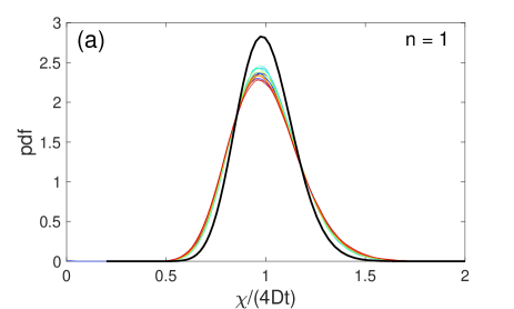
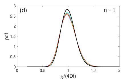
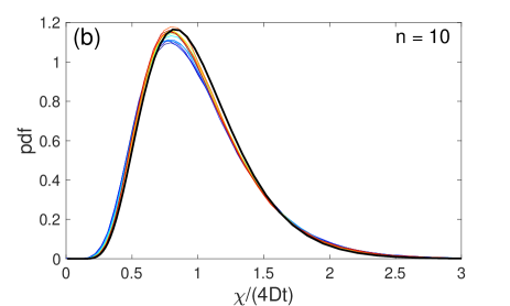
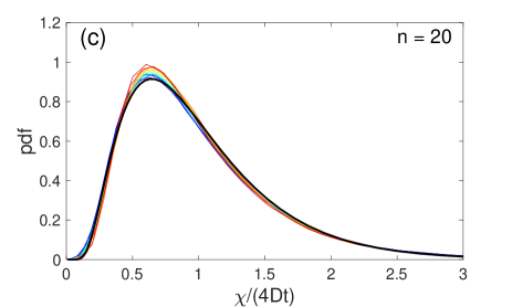
Figure 6: (Color online) (a,b,c) Probability density functions of the rescaled TAMSD, $\chi_{n,N}/(4Dt)$, with $N=100$, $t=n\delta$, and $n=1$ (a), $n=10$ (b), and $n=20$ (c), for 14 samples (thin lines), and the theoretical ones for Brownian motion (thick black line). Color of thin curves changes from dark blue for the lowest packing fraction $\phi$ to dark red for the highest one. (d) Probability density functions of the rescaled TAMSD with $N=100$, $t=n\delta$, and $n=1$, for 14 reshuffled samples.

In order to check the second reason of deviations (weak non-Gaussianity), the increments of all trajectories in each sample were randomly reshuffled to fully destroy auto-correlations, and then new artificial trajectories were constructed from these increments. If the original increments were correlated Gaussian variables with the same variance, such a procedure would yield independent identically distributed Gaussian variables so that the resulting trajectories would represent Brownian motion. In this case, a perfect agreement between empirical and theoretical curves would be expected. Figure 6(d) shows empirical and theoretical distributions of TAMSD at the lag time $n=1$ for reshuffled samples. The agreement is not perfect but is much better than in Fig. 6(a). Small residual deviations can potentially be attributed to weak non-Gaussianity of the distribution of increments.

III.7 Mean versus the most probable TAMSD

The nonsymmetric shape of the distribution of TAMSD implies that the mean value of the TAMSD is different from its mode, i.e., the most probable value or, equivalently, the position of the maximum of the PDF. This difference becomes particularly important for the analysis of single particle trajectories. When the sample of such individual trajectories is large, the empirical mean of TAMSD estimated from these trajectories is close to the expectation. In turn, when the TAMSD is estimated from few trajectories (or even from a single trajectory), it is more probable to observe a random realization near the maximum of the PDF. This issue, which was not relevant for symmetric distribution (e.g., a Gaussian distribution), may become an important bias in the analysis of TAMSD.

As discussed in Ref. Grebenkov11 , the distribution of TAMSD for Brownian motion is wider and more skewed for larger $n/N$. Moreover, the difference between the mean and the mode also grows with $n/N$. As suggested in Grebenkov11 , the distribution of TAMSD for Brownian motion and some other centered Gaussian processes (like fractional Brownian motion) can be accurately approximated by a generalized Gamma distribution, which has a simple explicit PDF

$$p(z)=\frac{z^{\nu-1}\exp(-a/z-z/b)}{2(ab)^{\nu/2}K_{\nu}(2\sqrt{a/b})}\quad(z>0),$$ (8)

with three parameters: $a\geq 0$, $b>0$, and $\nu\in{\mathbb{R}}$ (here $K_{\nu}(z)$ is the modified Bessel function of the second kind). The moments of this distribution can be expressed as

$$\langle[\chi_{n,N}]^{k}\rangle=(ab)^{k/2}\frac{K_{\nu+k}(2\sqrt{a/b})}{K_{\nu}(2\sqrt{a/b})}\quad(k=1,2,3,\ldots),$$ (9)

whereas the mode is

$$\chi_{n,N}^{\rm mode}=\frac{\sqrt{(1-\nu)^{2}b^{2}+4ab}-(1-\nu)b}{2}\,.$$ (10)

For a given empirical distribution of TAMSD, the first three moments, evaluated directly from the data, can be used to calculate the parameters $a$, $b$ and $\nu$ by solving numerically the system of three equations in Eqs. (9) for $k=1,2,3$. In other words, one does not need to fit the empirical distribution in order to get this approximation.

Figure 7 shows the pdf of the TAMSD for the trajectories with the lowest packing fraction, with the sample length $N=100$ and three lag times, $n=1$, $n=10$ and $n=20$ (shown by symbols). From these empirical data, we evaluated the first three moments and calculated the parameters $a$, $b$ and $\nu$ of the generalized gamma distribution (shown by lines). The excellent agreement validates the use of this theoretical approximation even for experimental trajectories.

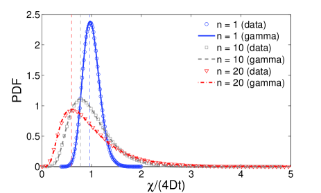
Figure 7: (Color online). Probability density functions of the rescaled TAMSD, $\chi_{n,N}/(4Dt)$, for the sample with the lowest packing fraction, with $N=100$, $t=n\delta$, and $n=1$ (blue circle), $n=10$ (gray squares), and $n=20$ (red triangles). Lines show the generalized gamma distribution $p(z)$ from Eq. (8) whose parameters were obtained from the first three moments (see the text): $a=3.27$, $b=0.03$, $\nu=28.13$ ($n=1$), $a=1.94$, $b=0.27$, $\nu=1.34$ ($n=10$), and $a=1.03$, $b=0.58$, $\nu=0.31$ ($n=20$). The modes of these distributions are shown by vertical dashed lines: $0.97$ ($n=1$), $0.78$ ($n=10$), and $0.60$ ($n=20$), whereas the mean is fixed to be $1$ by rescaling.

IV Conclusion

We proposed a macroscopic realization of planar Brownian motion by vertically vibrated disks. We performed a systematic statistical analysis of many random trajectories of individual disks. The distribution of one-step increments was shown to be almost Gaussian. Since small deviations at large increments increase with the disk packing fraction, they were attributed to inter-disk collisions. The velocity auto-correlation function was positive at the lag time $n=1$ and took negative values at $n>1$ that rapidly vanish with $n$. We also analyzed the behavior of the time averaged mean square displacement as a function of the lag time, and its fluctuations from one trajectory to another. We compared the empirical and theoretical distributions of TAMSD and revealed the sensitivity of this distribution at small lag times to eventual auto-correlations and weak non-Gaussianity. We also verified that the empirical distribution can be accurately approximated by the generalized Gamma distribution. Finally, we discussed distinctions between the mean TAMSD and the mode of its distribution. These well-controlled experimental data can serve for validating statistical tools developed for the analysis of single-particle trajectories in microbiology.

- (1) R. Brown, “A brief account of microscopical observations made in the months of June, July and August, 1827, on the particles contained in the pollen of plants; and on the general existence of active molecules in organic and inorganic bodies”, Edinburgh New Phil. J. 5, 358-371 (1828).
- (2) J. Perrin, “L’agitation moléculaire et le mouvement brownien”, Compt. Rendus Herbo. Seances Acad. Sci. Paris 146, 967 (1908).
- (3) J. Perrin, “Mouvement brownien et réalité moléculaire”, Ann. Chim. Phys. 18, 1-114 (1909).
- (4) E. Frey and K. Kroy, “Brownian motion: a paradigm of soft matter and biological physics”, Ann. Phys. (Leipzig) 14, 20 (2005).
- (5) D. S. Grebenkov, “NMR Survey of Reflected Brownian Motion”, Rev. Mod. Phys. 79, 1077-1137 (2007).
- (6) E. Sackmann, F. Keber, and D. Heinrich, “Physics of Cellular Movements”, Ann. Rev. Conden. Matt. Phys. 1, 257-276 (2010).
- (7) C. Bräuchle, D. C. Lamb, and J. Michaelis (Eds.), Single Particle Tracking and Single Molecule Energy Transfer, (Wiley-VCH, Weinheim, 2010).
- (8) H. M. Jaeger, S. R. Nagel, and R. P. Behringer, “Granular solids, liquids, and gases”, Rev. Mod. Phys. 68, 1259 (1996).
- (9) J. Choi, A. Kudrolli, R. R. Rosales, and M. Z. Bazant, “Diffusion and Mixing in Gravity-Driven Dense Granular Flows”, Phys. Rev. Lett. 92, 174301 (2004).
- (10) D. S. Grebenkov, M. P. Ciamarra, M. Nicodemi, and A. Coniglio, “Flow, Ordering and Jamming of Sheared Granular Suspensions”, Phys. Rev. Lett. 100, 078001 (2008).
- (11) W. Chen and K. To, “Unusual diffusion in a quasi-two-dimensional granular gas”, Phys. Rev. E 80, 061305 (2009).
- (12) C. Scalliet, A. Gnoli, A. Puglisi, and A. Vulpiani, “Cages and Anomalous Diffusion in Vibrated Dense Granular Media”, Phys. Rev. Lett. 114, 198001 (2015).
- (13) H. Qian, M. P. Sheetz, and E. L. Elson, “Single particle tracking. Analysis of diffusion and flow in two-dimensional systems”, Biophys. J. 60, 910-921 (1991).
- (14) D. Arcizet, B. Meier, E. Sackmann, J. O. Rädler, and D. Heinrich, “Temporal Analysis of Active and Passive Transport in Living Cells”, Phys. Rev. Lett. 101, 248103 (2008).
- (15) R. Metzler, V. Tejedor, J.-H. Jeon, Y. He, W. H. Deng, S. Burov, and E. Barkai, “Analysis of Single Particle Trajectories: From Normal to Anomalous Diffusion”, Acta Phys. Pol. B 40, 1315-1331 (2009).
- (16) X. Michalet, “Mean square displacement analysis of single-particle trajectories with localization error: Brownian motion in an isotropic medium”, Phys. Rev. E 82, 041914 (2010).
- (17) A. J. Berglund, “Statistics of camera-based single-particle tracking”, Phys. Rev. E 82, 011917 (2010).
- (18) X. Michalet and A. J. Berglund, “Optimal diffusion coefficient estimation in single-particle tracking”, Phys. Rev. E 85, 061916 (2012).
- (19) C. L. Vestergaard, P. C. Blainey, and H. Flyvbjerg, “Optimal estimation of diffusion coefficients from single-particle trajectories”, Phys. Rev. E 89, 022726 (2014).
- (20) N. Gal, D. Lechtman-Goldstein, and D. Weihs, “Particle tracking in living cells: a review of the mean square displacement method and beyond”, Rheol. Acta 52, 425-443 (2013).
- (21) E. Kepten, A. Weron, G. Sikora, K. Burnecki, and Y. Garini, “Guidelines for the Fitting of Anomalous Diffusion Mean Square Displacement Graphs from Single Particle Tracking Experiments”, PLoSONE 10, e0117722 (2015).
- (22) M. Magdziarz and A. Weron, “Anomalous diffusion: Testing ergodicity breaking in experimental data”, Phys. Rev. E 84, 051138 (2011).
- (23) Y. Lanoiselée and D. S. Grebenkov, “Revealing nonergodic dynamics in living cells from a single particle trajectory”, Phys. Rev. E 93, 052146 (2016).
- (24) Y. Lanoiselée and D. S. Grebenkov, “Unravelling intermittent features in single particle trajectories by a local convex hull method”, Phys. Rev. E 96, 022144 (2017).
- (25) J. Deseigne, S. Léonard, O. Dauchot, and H. Chaté, “Vibrated polar disks: spontaneous motion, binary collisions, and collective dynamics”, Soft Matter 8, 5629 (2012).
- (26) D. S. Grebenkov, “Probability Distribution of the Time-Averaged Mean-Square Displacement of a Gaussian Process”, Phys. Rev. E 84, 031124 (2011).
- (27) D. S. Grebenkov, “Optimal and sub-optimal quadratic forms for non-centered Gaussian processes”, Phys. Rev. E 88, 032140 (2013).
- (28) H. Cramér, Mathematical Methods of Statistics (Princeton University Press, 1946).
- (29) M. H. G. Duits, Y. Li, S. A. Vanapalli and F. Mugele, “Mapping of spatiotemporal heterogeneous particle dynamics in living cells”, Phys. Rev. E 79, 051910 (2009).
- (30) M. Otten, A. Nandi, D. Arcizet, M. Gorelashvili, B. Lindner, and D. Heinrich, “Local Motion Analysis Reveals Impact of the Dynamic Cytoskeleton on Intracellular Subdiffusion”, Biophys. J. 102, 758-767 (2012).
- (31) A. Nandi, D. Heinrich, and B. Lindner, “Distributions of diffusion measures from a local mean-square displacement analysis”, Phys. Rev. E 86, 021926 (2012).
- (32) M. J. Saxton, “Lateral diffusion in an archipelago. Single-particle diffusion”, Biophys. J. 64, 1766-1780 (1993).
- (33) M. J. Saxton, “Single-particle tracking: the distribution of diffusion coefficients”, Biophys. J. 72, 1744-1753 (1997).
- (34) A. Andreanov and D. S. Grebenkov, “Time-averaged MSD of Brownian motion”, J. Stat. Mech. P07001 (2012).
- (35) G. Sikora, M. Teuerle, A. Wylomanska, and D. S. Grebenkov, “Statistical properties of the anomalous scaling exponent estimator based on time averaged mean square displacement”, Phys. Rev. E 96, 022132 (2017).