Competing phases and topological excitations of spin-one pyrochlore antiferromagnets

Abstract

Most works on pyrochlore magnets deal with the interacting spin-1/2 local moments. We here study the spin-one local moments on the pyrochlore lattice, and propose a generic interacting spin model on a pyrochlore lattice. Our spin model includes the antiferromagnetic Heisenberg interaction, the Dzyaloshinskii-Moriya interaction and the single-ion spin anisotropy. We develop a flavor wave theory and combine with a mean-field approach to study the global phase diagram of this model and establish the relation between different phases in the phase diagram. We find the regime of the quantum paramagnetic phase where a degenerate line of the magnetic excitations emerges in the momentum space. We further predict the critical properties of the transition out of the quantum paramagnet to the proximate orders. The presence of quantum order by disorder in the parts of the ordered phases is then suggested. We point out the existence of degenerate and topological excitations in various phases. We discuss the relevance with fluoride pyrochlore material NaCaNi₂F₇ and explain the role of the spin-orbit coupling and the magnetic structures of the Ru-based pyrochlore A₂Ru₂O₇ and the Mo-based pyrochlore A₂Mo₂O₇.

I Introduction

Recently, there is a growing interest and effort in the frustrated magnetic systems with spin-one local moments, and interesting quantum phases and unconventional excitations have been predicted for frustrated spin-one systems Haldane (1983a, b); Affleck et al. (1987); Chen et al. (2011); Wang et al. (2015); Chen (2017a); Savary (2015); Wang et al. (2017). In particular, a chiral liquid phase with a finite vector chirality order has been obtained for the spin-one triangular lattice magnet Wang et al. (2017), Haldane phase like symmetry-protected topological phases have been suggested for three-dimensional spin-one systems Wang et al. (2015); Chamorro and McQueen (2017), spin liquid related physics and phenomenology has been explored for the layered triangular material Ba₃NiSb₂O₉ Cheng et al. (2011); Serbyn et al. (2011); Bieri et al. (2012); Xu et al. (2012); Chen et al. (2012); Hwang et al. (2013); Quilliam et al. (2016), and exotic excitations with degenerate band minima were established for the spin-one diamond lattice antiferromagnet Chen (2017a); Buessen et al. (2017). In this work, we turn our attention to the spin-one pyrochlore lattice antiferromagnet.

Pyrochlore antiferromagnet Gardner et al. (2010) is a stereotype of spin systems with geometrical frustration and potential quantum phases. In last decade or so, most efforts in the field were devoted to the rare-earth pyrochlore magnets where the relevant degrees of freedom are certain spin-orbital-entangled effective spin-1/2 local moments Gardner et al. (2010); Bramwell and Gingras (2001); Melko et al. (2001); Castelnovo1 et al. (2008); Molavian et al. (2007); Gingras and McClarty (2014); Savary and Balents (2016); Onoda and Tanaka (2010); Savary and Balents (2012); Lee et al. (2012); Savary and Balents (2013); Melko et al. (2001); Fukazawa et al. (2002); Bramwell et al. (2001); Gingras and McClarty (2014); Ross et al. (2009); Huang et al. (2014); Chen (2016); Wan and Tchernyshyov (2012); Li and Chen (2017); Yan et al. (2017); Savary et al. (2016); Savary and Balents (2013); Fennell et al. (2012); Yasui et al. (2002); Gardner et al. (2001); Hao et al. (2014); Chang et al. (2012); Kimura et al. (2013); Lhotel et al. (2014); Chang et al. (2014); Yasui et al. (2003); Ross et al. (2011); Shannon et al. (2012); Goswami et al. (2016); Arpino et al. (2017); Wen et al. (2017); MacLaughlin et al. (2015); Chen et al. (2014); Fu et al. (2017); Benton et al. (2012); Jaubert et al. (2015); Applegate et al. (2012); Dunsiger et al. (2011); Sibille et al. (2015); Taillefumier et al. (2017); Chen (2017b); Savary and Balents (2017); Chen (2017c). Due to the geometrical frustration and the bond-dependent anisotropic spin interaction Melko et al. (2001); Bramwell and Gingras (2001); Onoda and Tanaka (2010); Curnoe (2008); Onoda (2011), interesting magnetic phases and phenomena, quantum spin ice and $U(1)$ quantum spin liquid for example, have been proposed and explored Molavian et al. (2007); Savary and Balents (2012); Lee et al. (2012); Onoda and Tanaka (2010). This field is fertilized by the existence of the abundant rare-earth pyrochlore magnets with different magnetic ions. Recently, a new family of fluoride pyrochlore systems with the transition metal ions Fe²⁺, Co²⁺, Ni²⁺ and Mn²⁺ has been synthesized Krizan and Cava (2015, 2014); Ross et al. (2017); Sanders et al. (2017). Unlike the rare-earth $4f$ electrons whose interactions are usually quite small, these new systems, consisting of transition metal ions, have much stronger spin interactions. Moreover, spin-orbit coupling is less important in these systems, although spin-orbit coupling sometimes becomes active and modifies the local moment structure if there exists a partially filled $t_{2g}$ shell for the magnetic ions Witczak-Krempa et al. (2014).

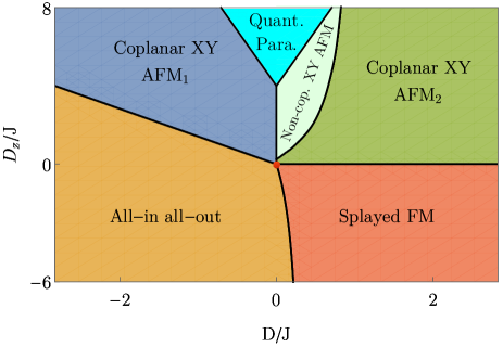
Figure 1: The phase diagram of our generic spin model for the spin-1 pyrochlore system. Here, the Heisenberg exchange $J$ is set to be antiferromagnetic with ${J>0}$. “Quant Para” refers to the quantum paramagnetic phase. The details of the ordered phases are explained in the main text. The (red) dot is the Heisenberg point of the model. A similar phase diagram with the ferromagnetic Heisenberg exchange is found in the Appendix E.

Just like the fundamental distinction between the half-integer and the integer spin moments for one dimensional spin chains that was pointed out by F.D.M. Haldane Haldane (1983a, b), the physical properties of the half-integer spin and the integer spin moments on the pyrochlore lattice are expected to be quite different. In fact, for the rare-earth pyrochlore magnets, such a distinction has already been manifested in the Kramers doublet system and the non-Kramers doublet system where the non-Kramers doublet originates from integer spin and supports magnetic quadrupolar order Onoda and Tanaka (2010); Lee et al. (2012); Chen (2016). Since most works in this field are dealing with effective spin-1/2 pyrochlores, it is valuable to consider the physics of the spin-1 pyrochlores.

Among the existing fluoride pyrochlores, Co²⁺ and Mn²⁺ have half-integer spin moments while Ni²⁺ and Fe²⁺ have integer spin moments Krizan and Cava (2015, 2014); Ross et al. (2017); Sanders et al. (2017). From the conventional wisdom, when the spin moment is large, the system tends to behave more classically. For geometrically frustrated systems, however, the spin-one local moments may occasionally give rise to quantum phenomena. Indeed, in the Ni-based fluoride pyrochlore NaCaNi₂F₇, spin-ordering-related features were not found in the thermodynamic measurement down to the spin glassy transition at $3.6$K that is attributed to the possible bond randomness, although the system has the Curie-Weiss temperature $-129$K Krizan and Cava (2015). Apart from this new material, the spin-one pyrochlores have already been suggested for the Ru-based pyrochlore A₂Ru₂O₇ and the Mo-based pyrochlore A₂Mo₂O₇, despite the fact that the stronger spin-orbit coupling of the $4d$ electrons may be more important in these two systems. Partly motivated by these experiments and more broadly about the physics of the spin-one moments, in this paper, we study the generic spin model and the magnetic properties of the spin-one local moments on the pyrochlore lattice.

We point out that, in addition to the Heisenberg model that is usually assumed for the $3d$ transition metal ions and sometimes for the $4d$ transition metal ions, there exist the on-site single-ion spin anisotropy and the antisymmetric Dyzaloshinskii-Moriya interaction. Our phase diagram is summarized in Fig. 1. In our approach, we start from the quantum paramagnetic ground state in the strong single-ion spin anisotropic limit and explore the instability of this quantum state as the Heisenberg exchange and the Dyzaloshinskii-Moriya interaction are switched on. Mostly relying on a flavor wave theory, we access the phase transitions out of this quantum paramagnetic state and explore the properties of criticalities. Inside the ordered phases, we implement the usual mean-field theory and establish the phase diagram on the ordered side. We further identify the region on the ordered side where there exist continuous degeneracies of the ground state manifold at the mean-field level. The quantum fluctuation is studied and lifts the continuous degeneracies. The magnetic excitations in different phases are also discussed.

The following parts of the paper are organized as follows. In Sec. II, we introduce the model Hamiltonian. In Sec. III, we use the flavor wave theory and study the magnetic excitation and the instability of the quantum paramagnetic phase. In Sec. IV, we focus on the ordered side and study the magnetic properties of the magnetic orders. Finally in Sec. V, we summarize the theoretical prediction and the physical properties of the phase diagram, discuss the materials’ relevance, and make an extension to spin-3/2 pyrochlores.

II Model Hamiltonian

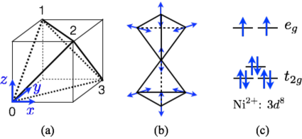
Figure 2: (a) The four sublattices and the unit cell of the pyrochlore lattice. (b) The (blue) arrows define the local $z$ or $\langle 111\rangle$ axis. (c) The electron configuration of the Ni²⁺ ion in NaCaNi₂F₇. While the $e_{g}$ orbitals remain degenerate under the D_3d point group, the $t_{2g}$ orbitals would be broken into $a_{1g}$ and two-fold degenerate $e_{g}^{\prime}$ orbitals. The relative energies of $a_{1g}$ and $e_{g}^{\prime}$ orbitals are unknown, and we place $a_{1g}$ at a higher energy in the figure. The ${S=1}$ nature of the Ni²⁺ local moment holds for either distribution of the $a_{1g}$ and $e_{g}^{\prime}$ orbitals.

We start from the local moment physics of the Ni²⁺ ion in NaCaNi₂F₇. Although the starting point here is specific to NaCaNi₂F₇, the physical model itself applies broadly to other spin-one pyrochlore systems, and we merely present the model through the specific case of NaCaNi₂F₇. The Ni²⁺ ion has a $3d^{8}$ electron configuration. In the octahedral crystal field environment of NaCaNi₂F₇, the six electrons occupy the lower $t_{2g}$ orbitals, and the remaining two electrons occupy the upper $e_{g}$ orbitals and form a spin ${S=1}$ local moment. There is no orbital degeneracy here. We propose the following spin model for the interaction between the local moments. The minimal spin Hamiltonian is given as Onoda (2011),

$$H = \sum_{\langle ij\rangle}\big{[}J{\boldsymbol{S}}_{i}\cdot{\boldsymbol{S}}_{j}+{\boldsymbol{D}}_{ij}\cdot({\boldsymbol{S}}_{i}\times{\boldsymbol{S}}_{j})\big{]}$$ (1)

$$+\sum_{i}D_{z}({\boldsymbol{S}}_{i}\cdot\hat{z}_{i})^{2},$$

where ${\boldsymbol{D}}_{ij}$ is the bond-dependent vector that defines the antisymmetric Dzyaloshinskii-Moriya interaction Elhajal et al. (2005). For the 01 bond in Fig. 2a, we have

$${\boldsymbol{D}}_{01}=(0,\frac{D}{\sqrt{2}},-\frac{D}{\sqrt{2}}),$$ (2)

and ${\boldsymbol{D}}_{ij}$’s on other bonds are readily obtained from the lattice symmmetry. The $D_{z}$ term is the single-ion spin anisotropy allowed by the D_3d point group symmetry of the pyrochlore lattice, and $\hat{z}_{i}$ is the local $\langle 111\rangle$ axis that is defined locally for each pyrochlore sublattice. Even though the Dzyaloshinskii-Moriya interaction arises from the first order effect of the spin-orbit coupling and the single-ion spin anisotropy arises from the second order effect of the spin-orbit coupling, it does not necessarily indicate the single-ion anisotropy is weaker than the Dzyaloshinskii-Moriya interaction. In fact, ignoring the effect from Hund’s coupling, one has the following results Maekawa et al. (2004)

$$|D_{ij}|/J \sim \mathcal{O}(\lambda/\Delta),$$ (3)

$$|D_{z}|/\Delta \sim \mathcal{O}(\lambda^{2}/\Delta^{2}),$$ (4)

where $\lambda$ is the spin-orbit coupling and $\Delta$ is the crystal electric field splitting between the $t_{2g}$ and the $e_{g}$ manifolds and can be much larger than the superexchange interaction $J$. As a result, whether $\lambda$ appears as the linear order or as the second order cannot be used to argue for the relative magnitudes of $|D_{ij}|$ and $D_{z}$. We include both couplings in our model Hamiltonian. We have neglected the pseudo-dipolar interactions, as they are subleading compared to the Dzyaloshinskii-Moriya interaction for the $3d$ transition metal ions without any orbital degeneracy Moriya (1960). The pseudo-dipolar interactions, however, may become important for the $4d$ transition metal ions.

III Flavor wave theory for quantum paramagnet

Our minimal model contains three different interactions. The quantum ground state of the Heisenberg model is one of the hardest problems in quantum magnetism, so it is not so profitable to start from there. Instead, we start from the strong single-ion spin anisotropy limit with ${D_{z}>0}$ where the ground state is a simple product state of the quantum paramagnet with

$$|\text{quantum paramagnet}\rangle=\prod_{i}|{S^{z}_{i}\equiv{\boldsymbol{S}}_{i}\cdot\hat{z}_{i}=0}\rangle.$$ (5)

This state is impossible for the half-integer spin local moments as there is always Kramers’ degeneracy. From this well-understood limit, we turn on the exchange interaction and study the evolution of the magnetic excitation and the instability.

For our convenience, we first rewrite the spin Hamiltonian in the local coordinate basis since the single-ion anisotropy is defined locally. Under the local coordinate systems that are defined in the Appendix B, our spin model reduces to Onoda (2011)

$$H = \sum_{\langle ij\rangle}\big{[}J_{zz}S_{i}^{z}S_{j}^{z}+J_{\pm}(S^{+}_{i}S^{-}_{j}+h.c.)+J_{\pm\pm}(\gamma_{ij}S^{+}_{i}S^{+}_{j}$$ (6)

$$\quad+\gamma_{ij}^{\ast}S^{-}_{i}S^{-}_{j})+J_{z\pm}(\xi_{ij}S_{i}^{z}S_{j}^{+}+\xi_{ij}S_{i}^{+}S_{j}^{z}+h.c.)\big{]}$$

$$\quad+\sum_{i}D_{z}(S_{i}^{z})^{2},$$

where these spin operators, $S^{z}_{i},S^{+}_{i},S^{-}_{i}$, are defined in the local coordinate system for each sublattice. Note the exchange part of the model has the general form as the one for the Kramers doublet on the pyrochlore lattice, and the bond dependent phase variables $\gamma_{ij}$ and $\xi_{ij}$ where $\gamma_{ij}$ takes $1,e^{i2\pi/3},e^{-i2\pi/3}$ for the bonds on different planes and ${\xi_{ij}=-\gamma_{ij}^{\ast}}$. The relation between the couplings in the above equation and the couplings in Eq. (1) is listed in Appendix B. In the following, we will focus our analysis on this form of the model.

III.1 Flavor wave representation

This quantum paramagnet has no long-range magnetic order, and the conventional Holstein-Primarkoff spin-wave theory cannot be directly applied at all. For our purpose, we invoke so-called flavor wave theory, that was first developed in Ref. Joshi et al., 1999 for the $SU(4)$ spin-orbital model Li et al. (1998), and properly adjust the formulation to our case. We define the states in the Hilbert space as

$$|m\rangle_{i}\equiv|{S^{z}_{i}=m}\rangle,$$ (7)

where ${m=0,\pm 1}$, and the elementary operator is then given as $S^{n}_{m}(i)\equiv|m\rangle_{i}\langle n|_{i}$. For the quantum paramagnet, we introduce the following flavor-wave representation,

$$S^{0}_{0}(i) = 1-a^{\dagger}_{1}(i)a_{1}(i)-a^{\dagger}_{\bar{1}}(i)a^{\phantom{\dagger}}_{\bar{1}}(i),$$ (8)

$$S^{0}_{1}(i) = a^{\dagger}_{1}(i)\big{[}1-a^{\dagger}_{1}(i)a_{1}(i)-a^{\dagger}_{\bar{1}}(i)a^{\phantom{\dagger}}_{\bar{1}}(i)\big{]}^{\frac{1}{2}},$$ (9)

$$S^{0}_{\bar{1}}(i) = a^{\dagger}_{\bar{1}}(i)\big{[}1-a^{\dagger}_{1}(i)a_{1}(i)-a^{\dagger}_{\bar{1}}(i)a^{\phantom{\dagger}}_{\bar{1}}(i)\big{]}^{\frac{1}{2}},$$ (10)

$$S^{1}_{\bar{1}}(i) = a^{\dagger}_{\bar{1}}(i)a^{\phantom{\dagger}}_{1}(i),$$ (11)

$$S^{1}_{1}(i) = a^{\dagger}_{1}(i)a^{\phantom{\dagger}}_{1}(i),$$ (12)

$$S^{\bar{1}}_{\bar{1}}(i) = a^{\dagger}_{\bar{1}}(i)a^{\phantom{\dagger}}_{\bar{1}}(i),$$ (13)

where $a^{\dagger}_{1}(i),a^{\dagger}_{\bar{1}}(i)$ create magnetic excitation from $|0\rangle_{i}$ to $|1\rangle_{i},|{-1}\rangle_{i}$, respectively. Here we have introduced two flavors of the boson operators. This is very different from the usual Holstein-Primakoff transformation where only one boson is introduced to describe the quantum fluctuation of the magnetic order. The underlying reason is due to the particular form of the Hamiltonian and the quantum paramagnetic ground state that allow the excitations of the $|1\rangle_{i},|{-1}\rangle_{i}$ states to be equally important. As a consequence, the excitation spectra for this quantum paramagnet should have eight bands, rather than the four bands in the usual Holstein-Primakoff spin wave theory. Moreover, since the model has no continuous symmetry, the magnetic excitation should be fully gapped.

III.2 Linear flavor wave theory

To carry out the actual calculation of the excitation spectra, we replace the physical spin operators using the flavor wave transformation and keep the Hamiltonian to the quadratic orders in the boson operators. The resulting flavor wave Hamiltonian is given as

$$H_{\text{fw}}=\sum_{\boldsymbol{k}}\Psi_{{\boldsymbol{k}}}^{\dagger}M({\boldsymbol{k}})\Psi_{{\boldsymbol{k}}}^{\phantom{\dagger}},$$ (14)

where

$$\Psi_{{\boldsymbol{k}}} \equiv \big{(}a_{{\boldsymbol{k}}01}^{\phantom{\dagger}},a_{{\boldsymbol{k}}0\bar{1}}^{\phantom{\dagger}},a_{{\boldsymbol{k}}11}^{\phantom{\dagger}},a_{{\boldsymbol{k}}1\bar{1}}^{\phantom{\dagger}},a_{{\boldsymbol{k}}21}^{\phantom{\dagger}},a_{{\boldsymbol{k}}2\bar{1}}^{\phantom{\dagger}},a_{{\boldsymbol{k}}31}^{\phantom{\dagger}},a_{{\boldsymbol{k}}3\bar{1}}^{\phantom{\dagger}},$$

$$a_{\bar{\boldsymbol{k}}01}^{\dagger},a_{\bar{\boldsymbol{k}}0\bar{1}}^{\dagger},a_{\bar{\boldsymbol{k}}11}^{\dagger},a_{\bar{\boldsymbol{k}}1\bar{1}}^{\dagger},a_{\bar{\boldsymbol{k}}21}^{\dagger},a_{\bar{\boldsymbol{k}}2\bar{1}}^{\dagger},a_{\bar{\boldsymbol{k}}31}^{\dagger},a_{\bar{\boldsymbol{k}}3\bar{1}}^{\dagger}\big{)}^{T},$$

and $M({\boldsymbol{k}})$ is a $16\times 16$ matrix. Here $\bar{\boldsymbol{k}}\equiv-{\boldsymbol{k}}$. Due to the choice of notation, $M({\boldsymbol{k}})$ can be written in block form as

$$M(\boldsymbol{k})=\begin{pmatrix}M_{1}(\boldsymbol{k})&M_{2}(\boldsymbol{k})\\ M_{2}^{*}(\boldsymbol{k})&M_{1}^{*}(\boldsymbol{k})\end{pmatrix},$$ (16)

where $M_{1}(\boldsymbol{k})$ and $M_{2}(\boldsymbol{k})$ are $8\times 8$ matrices and satisfy $M_{1}^{\dagger}(\boldsymbol{k})=M_{1}(\boldsymbol{k})$, $M_{2}^{T}(\boldsymbol{k})=M_{2}(\boldsymbol{k})$. The detailed matrix elements are listed in the Appendix C.

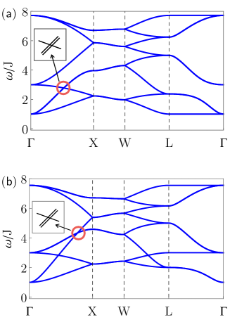
Figure 3: The (gapped) magnetic excitations in the quantum paramagnetic phase from the linear flavor wave theory. Notice the existence of the triply degenerate nodes (red circle) in the spectrum, see the main text for detailed discussion. In the inset of (a), the two-fold degenerate bands are split artificially for demonstration. The parameters are (a) ${D=-0.14J,D_{z}=5J}$; (b) ${D=0.14J,D_{z}=5J}$. The high symmetry momenta in the Brillouin zone are defined as ${\Gamma=(0,0,0)}$, ${\text{X}=(0,2\pi,0)}$, ${\text{W}=(\pi,2\pi,0)}$, ${\text{L}=(\pi,\pi,\pi)}$.

In Fig. 3, we plot the linear flavor wave dispersion for the specific choices of the couplings within the quantum paramagnetic phase. As we expect, there are eight bands of the magnetic excitations that are fully gapped. Besides the doubled number of the bands, we notice other unusual properties of the excitations. We find that, in the ${D<0}$ region of the quantum paramagnetic phase, the minima of the magnetic excitations develop a line of degeneracies from $\Gamma$ to $L$ in the momentum space. In the ${D>0}$ region of the quantum paramagnetic phase, the band minima of the two lowest bands touch at the $\Gamma$ point with an accidental two-fold degeneracy in the spin space. Both the momentum space degeneracy and the spin space degeneracy are not protected by any symmetry of the spin Hamiltonian. We expect the emergent degeneracy to be lifted when we go beyond the linear flavor wave theory and include the interaction between the flavor bosons.

III.3 Critical properties from flavor wave theory

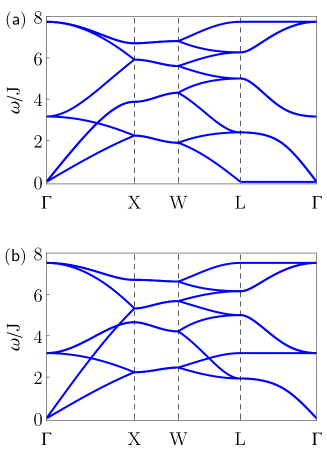
Figure 4: The magnetic excitations on the phase boundary of the quantum paramagnet, obtained from the linear flavor wave theory. The excitation gap is closed. The parameters are (a) ${D=-0.17J}$, ${D_{z}=5J}$; (b) ${D=0.17J}$, ${D_{z}=5J}$.

As we further increase the exchange interaction from the quantum paramagnet, the gap of the magnetic excitations gradually diminishes. Eventually, as the gap is closed, phase transition happens and the system develops magnetic orders. To understand the critical properties, we examine the transition from the flavor wave theory. In the ${D<0}$ region, the degenerate modes along the momentum line from $\Gamma$ to $L$ become critical at the same time as the gap is closed, see Fig. 4(a). Because of the line degeneracy, there is an enhanced density of states at low energies at the criticality, and we would expect the specific heat ${C_{v}\sim T^{2}}$ behavior at low temperatures from the mean-field theory. The zero-temperature limit of the specific heat should be modified because the fluctuations break the momentum space degeneracy and lead to discrete degeneracy. In the ${D>0}$ region, as the system approaches the criticality, only the $\Gamma$ point becomes critical, see Fig. 4(b), and we expect a simple ${C_{v}\sim T^{3}}$ at the mean-field level and a logarithmic correction when the fluctuations beyond the mean-field are included.

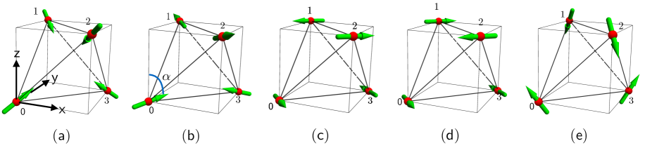
Figure 5: Representative configurations of the magnetic ordered states. (a) All-in-all-out. (b) Splayed FM. The splay angle is labeled by $\alpha$. For this configuration, $\alpha=74.2^{\circ}$. (c) Coplanar XY AFM₁. (d) Coplanar XY AFM₂. (e) Non-coplanar XY AFM.

III.4 Flavor wave excitations

In the flavor wave excitation spectrum, there exist triply degenerate nodes along $\Gamma$-X and symmetry equivalent momentum directions, indicated by red circles in Fig. 3.

In the insets of Fig. 3, we sketch that there are two-fold degenerate bands near the triply degenerate nodes. This two-fold band degeneracy is protected by a glide symmetry, which can be realized by a reflection in (100) plane followed by a fractional translation $\left({1}/{2},{1}/{4},{3}/{4}\right)$ in our origin choice (see Fig. 2(a)). This symmetry operation keeps the $\Gamma$-X line invariant and permutes the sublattices as $0\leftrightarrow 1$ and $2\leftrightarrow 3$. Since a generic field removes the glide symmetry and lifts the two-fold band degeneracy, one can apply an external magnetic field to open a gap in the position of a triply degenerate node.

The triply degenerate nodes have been previously discussed in the electronic systemsBradlyn et al. (2016); Weng et al. (2016); Zhu et al. (2016); Lv et al. (2017). Unlike the cases for the electronic systems where the modes at the nodes become unconventional quasiparticles if the Fermi level is tuned to the nodes, these excitations occur at the finite energies for the bosonic flavor waves.

We mention that in Fig. 3(b), there exist doubly degenerate touchings along $\Gamma$-X, W-L and symmetry equivalent momentum directions. These touchings belong to a nodal surface rather than being isolated nodes, we will discuss their properties in future works.

IV Mean-field theory

To study the proximate magnetic order out of the quantum paramagnetic phase, one natural approach would simply follow the flavor wave theory that we have introduced in the previous section and study the condensation of the critical flavor wave modes. This is certainly feasible and requires including the interactions between the flavor wave modes that lift the degeneracy of the low-energy modes. We, however, implement a mean-field theory in this section. This is justified since the system develops magnetic orders in the parameter regimes that we are interested. This mean-field approach works best deep on the ordered side. In the mean-field theory, we simply replace the spin operator with the mean-field order parameter and optimize the mean-field Hamiltonian,

$$\langle H\rangle = \sum_{\langle ij\rangle}J\,{\boldsymbol{m}}_{i}\cdot{\boldsymbol{m}}_{j}+{\boldsymbol{D}}_{ij}\cdot({\boldsymbol{m}}_{i}\times{\boldsymbol{m}}_{j})$$ (17)

$$+\sum_{i}D_{z}({\boldsymbol{m}}_{i}\cdot\hat{z}_{i})^{2},$$

under the local constraint ${|{\boldsymbol{m}}_{i}|^{2}=S^{2}}$. The mean-field ground state can then be found using the simple Luttinger-Tisza method. Our results are summarized and displayed in Fig. 1 and Fig. 5. All of these orders support an ordering wavevector ${{\boldsymbol{Q}}={\boldsymbol{0}}}$ where the magnetic unit cell coincides with the crystal unit cell. In the following, we describe the magnetic orders in details. Since we are interested in magnetic orders in this section, our results will be presented from bottom to top and from left to right in the phase diagram of Fig. 1.

IV.1 All-in all-out AFM

In the lower left region of the phase diagram, the “all-in all-out” magnetic order is stabilized. This is understood as follows. The easy-axis anisotropy favors the spins to be aligned with the local $\hat{z}$ direction, and the Heisenberg interaction requires the vector addition of the spins from the four sublattices to be zero. The Dzyaloshinskii-Moriya interaction is less obvious, but naturally favors non-collinear spin configurations. Simple diagonalization of the Dzyaloshinskii-Moriya interaction term directly gives the “all-in all-out” spin configuration. Therefore, all three interactions in the Hamiltonian are optimized by the “all-in all-out” spin configuration. Since the Dzyaloshinskii-Moriya interaction favors this ground state, this “all-in all-out” state extends further into the easy-plane anisotropic regime with $D_{z}>0$. As the local $\hat{z}$ direction is a three-fold rotational axis, this symmetry operation does not generate new ground states, and the ground state spin configuration merely has a $\mathbb{Z}_{2}$ degeneracy from the time-reversal transformation.

IV.2 Splayed FM

In the lower right region of the phase diagram, the “splayed ferromagnet” (“splayed FM”) is stabilized. One such spin configuration is given in Fig. 5(b) and parameterized as

$$\left\{\begin{array}[]{l}{\boldsymbol{m}}_{0}=(\frac{\sin\alpha}{\sqrt{2}},\frac{\sin\alpha}{\sqrt{2}},\cos\alpha),\\[11.38092pt] {\boldsymbol{m}}_{1}=(-\frac{\sin\alpha}{\sqrt{2}},\frac{\sin\alpha}{\sqrt{2}},\cos\alpha),\\[11.38092pt] {\boldsymbol{m}}_{2}=(\frac{\sin\alpha}{\sqrt{2}},-\frac{\sin\alpha}{\sqrt{2}},\cos\alpha),\\[11.38092pt] {\boldsymbol{m}}_{3}=(-\frac{\sin\alpha}{\sqrt{2}},-\frac{\sin\alpha}{\sqrt{2}},\cos\alpha),\end{array}\right.$$ (22)

where ${\boldsymbol{m}}_{\mu}$ refers to the magnetic order on the $\mu$-th sublattice, and the “splay angle” $\alpha$ is found to be

$$\alpha=\arctan\frac{D_{z}^{\prime}-[8D_{z}^{2}+{D^{\prime}_{z}}^{2}]^{\frac{1}{2}}}{2\sqrt{2}D_{z}},$$ (23)

here ${D^{\prime}_{z}\equiv D_{z}-12J-3\sqrt{2}D}$. There is a ferromagnetic component $\cos\alpha$ along the global $z$ direction.

Other equivalent ground state spin configurations can be obtained by lattice symmetry operations, and we have the other ground states as

$$\left\{\begin{array}[]{l}{\boldsymbol{m}}_{0}=(\frac{\sin\alpha}{\sqrt{2}},\cos\alpha,\frac{\sin\alpha}{\sqrt{2}}),\\[11.38092pt] {\boldsymbol{m}}_{1}=(-\frac{\sin\alpha}{\sqrt{2}},\cos\alpha,\frac{\sin\alpha}{\sqrt{2}}),\\[11.38092pt] {\boldsymbol{m}}_{2}=(-\frac{\sin\alpha}{\sqrt{2}},\cos\alpha,-\frac{\sin\alpha}{\sqrt{2}}),\\[11.38092pt] {\boldsymbol{m}}_{3}=(\frac{\sin\alpha}{\sqrt{2}},\cos\alpha,-\frac{\sin\alpha}{\sqrt{2}}),\end{array}\right.$$ (28)

and

$$\left\{\begin{array}[]{l}{\boldsymbol{m}}_{0}=(\cos\alpha,\frac{\sin\alpha}{\sqrt{2}},\frac{\sin\alpha}{\sqrt{2}}),\\[11.38092pt] {\boldsymbol{m}}_{1}=(\cos\alpha,-\frac{\sin\alpha}{\sqrt{2}},-\frac{\sin\alpha}{\sqrt{2}}),\\[11.38092pt] {\boldsymbol{m}}_{2}=(\cos\alpha,-\frac{\sin\alpha}{\sqrt{2}},\frac{\sin\alpha}{\sqrt{2}}),\\[11.38092pt] {\boldsymbol{m}}_{3}=(\cos\alpha,\frac{\sin\alpha}{\sqrt{2}},-\frac{\sin\alpha}{\sqrt{2}}).\end{array}\right.$$ (33)

Together with the time reversal symmetry, there exist a ${\mathbb{Z}_{3}\times{\mathbb{Z}}_{2}}$ degeneracy. This state supports a weak ferromagnetism along one cubic axis and antiferromagnetism in the remaining two directions. Clearly, when $|D_{z}|$ is dominant, the spins should be aligned with the local $\hat{z}$ direction, and the Dzyaloshinskii-Moriya interaction then favors “two-in two-out” spin configurations in this case.

In the strong $D_{z}$ limit, the splay angle ${\alpha\approx 54.7^{\circ}}$, and the ground state is exactly the “two-in two-out” spin ice configurations. In contrast, in the weak $D_{z}$ limit, ${\alpha=90^{\circ}}$ and the ground state becomes coplanar. This means the “two-in two-out” spin ice configurations are smoothly connected to coplanar states in this “splayed FM” regime.

In general, in this parameter regime, the interactions cannot be optimized simultaneously. However, taking three interactions together, we are able to find the “splayed FM” as the ground state. This “splayed FM” was actually proposed for the well-known quantum spin ice candidate materials Yb₂Sn₂O₇ and Yb₂Ti₂O₇ Yaouanc et al. (2013); Thompson et al. (2017), so we adopt the name from there. We note that the splay angle $\alpha$ can only take value from $54.7^{\circ}$ to $90^{\circ}$ for the “splayed FM” regime with antiferromagnetic Heisenberg exchange. When the Heisenberg exchange becomes ferromagnetic, $\alpha$ can take a larger parameter regime (see Appendix E).

IV.3 Coplanar XY AFM₁

In the upper left region of the phase diagram, we obtain a coplanar antiferromagnetic spin ground state and dub it “coplanar XY AFM₁”. Here ‘XY’ refers to the $xy$ plane of the local coordinate system. One such spin state is depicted in Fig. 5(c) and is given as

$$\left\{\begin{array}[]{l}{\boldsymbol{m}}_{0}=\frac{1}{\sqrt{2}}(1,\bar{1},0),\\[11.38092pt] {\boldsymbol{m}}_{1}=\frac{1}{\sqrt{2}}(\bar{1},\bar{1},0),\\[11.38092pt] {\boldsymbol{m}}_{2}=\frac{1}{\sqrt{2}}(1,{1},{0}),\\[11.38092pt] {\boldsymbol{m}}_{3}=\frac{1}{\sqrt{2}}(\bar{1},{1},0).\end{array}\right.$$ (38)

The spins are perpendicular to the local $\hat{z}$ direction of the relevant sublattice and orient antiferromagnetically within the same plane globally. This explains the use of the “coplanar XY AFM₁”. This “coplanar XY AFM₁” ground state occurs when ${D_{z}>\sqrt{2}|D|}$ as one further increases the easy-plane anisotropy from the “all-in all-out” phase. This “coplanar XY AFM₁” phase is in the easy-plane anisotropic limit, and the spins prefer to orient in the local $xy$ plane. The in-plane spin configuration is able to content both the easy-plane spin anisotropy and the Heisenberg exchange. Since it is known from the previous subsection that the Dzyaloshinskii-Moriya interaction is optimized by the “all-in all-out” state for ${D<0}$. The particular spin configuration of the “coplanar XY AFM₁” state is obtained because the easy-plane anisotropy wins over the Dzyaloshinskii-Moriya interaction such that the Dzyaloshinskii-Moriya interaction is optimized within the manifold of coplanar spin configurations only.

Applying the lattice symmetry operations, we generate two equivalent spin configurations with

$$\left\{\begin{array}[]{l}{\boldsymbol{m}}_{0}=\frac{1}{\sqrt{2}}(0,1,\bar{1}),\\[11.38092pt] {\boldsymbol{m}}_{1}=\frac{1}{\sqrt{2}}(0,\bar{1},{1}),\\[11.38092pt] {\boldsymbol{m}}_{2}=\frac{1}{\sqrt{2}}(0,\bar{1},\bar{1}),\\[11.38092pt] {\boldsymbol{m}}_{3}=\frac{1}{\sqrt{2}}(0,{1},{1}),\end{array}\right.$$ (43)

and

$$\left\{\begin{array}[]{l}{\boldsymbol{m}}_{0}=\frac{1}{\sqrt{2}}(1,0,\bar{1}),\\[11.38092pt] {\boldsymbol{m}}_{1}=\frac{1}{\sqrt{2}}(\bar{1},0,\bar{1}),\\[11.38092pt] {\boldsymbol{m}}_{2}=\frac{1}{\sqrt{2}}(\bar{1},0,{1}),\\[11.38092pt] {\boldsymbol{m}}_{3}=\frac{1}{\sqrt{2}}({1},0,{1}).\end{array}\right.$$ (48)

Again from the time reversal symmetry, we have a $\mathbb{Z}_{3}\times\mathbb{Z}_{2}$ degeneracy for the ground state.

IV.4 Coplanar XY AFM₂

In the upper right region (both the “coplanar XY AFM₂” and “non-coplanar XY AFM”) of the phase diagram, we find an extensively degenerate mean-field ground state, and all the three interactions are optimized at the same time. The extensive degeneracy is parametrized by a $U(1)$ angular variable $\theta$, and the ground state spin configuration is given as

$${\boldsymbol{m}}_{\mu}=\hat{x}_{\mu}\cos\theta+\hat{y}_{\mu}\sin\theta,$$ (49)

with ${\theta\in[0,2\pi)}$. Our spin Hamiltonian does not have any continuous symmetry, thus the continuous degeneracy is not the symmetry property of the Hamiltonian but is accidental. We expect this continuous degeneracy to be lifted by quantum fluctuation. This quantum order by disorder effect has been previously explored in the effective spin-1/2 pyrochlore material Er₂Ti₂O₇ Savary et al. (2012); Zhitomirsky et al. (2012, 2014). We here study this quantum mechanical effect in the spin-1 pyrochlore system. We first introduce the Holstein-Primakoff transformation for the spin operators,

$${\boldsymbol{S}}_{i}\cdot{\boldsymbol{m}}_{i}=S-b^{\dagger}_{i}b^{\phantom{\dagger}}_{i},$$ (50)

$${\boldsymbol{S}}_{i}\cdot\hat{z}_{i}=\frac{\sqrt{2S}}{2}(b^{\phantom{\dagger}}_{i}+b^{\dagger}_{i}),$$ (51)

$${\boldsymbol{S}}_{i}\cdot({\boldsymbol{m}}_{i}\times\hat{z}_{i})=\frac{\sqrt{2S}}{2i}(b^{\phantom{\dagger}}_{i}-b^{\dagger}_{i}).$$ (52)

Substituting the spin operators with the Holstein-Primakoff bosons and keeping the boson terms up to quadratic order, we have the linear spin wave Hamiltonian (see Appendix D),

$$H_{\text{sw}} = \sum_{\boldsymbol{k}}\sum_{\mu\nu}\bigg{[}\frac{D_{z}}{2}\delta_{\mu\nu}+A_{\mu\nu}({\boldsymbol{k}})b_{{\boldsymbol{k}}\mu}^{\dagger}b_{{\boldsymbol{k}}\nu}^{\phantom{\dagger}}$$ (53)

$$+\left(B_{\mu\nu}({\boldsymbol{k}})b_{{\boldsymbol{k}}\mu}^{\dagger}b_{-{\boldsymbol{k}}\nu}^{\dagger}+\text{h.c.}\right)\bigg{]}+E_{\text{mf}},$$

where $E_{\text{mf}}$ is the mean-field energy of the ground state. The quantum zero point energy is found to be

$$\Delta E=\sum_{\boldsymbol{k}}\sum_{\mu}\frac{1}{2}\Big{[}\omega_{\mu}({\boldsymbol{k}})-A_{\mu\mu}({\boldsymbol{k}})+D_{z}\Big{]},$$ (54)

here $\omega_{\mu}({\boldsymbol{k}})$ is the spin wave excitation. In Fig. 6, we plot the quantum zero point energy and find that the minima are realized at

$$\theta=\frac{n\pi}{3}+\frac{\pi}{6},$$ (55)

for ${n\in\mathbb{Z}}$, see Fig. 6(a). One such spin configuration is displayed in Fig. 5(d), and all the spins orient antiferromagnetically within the same plane. We dub this phase “coplanar XY AFM₂”.

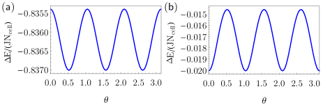
Figure 6: Order by quantum disorder in the upper right region of the phase diagram. Coplanar XY AFM₂ and Non-coplanar XY AFM are separated by different (a) In coplanar XY AFM₂, the minima of zero point energy are realized at $\theta={n\pi}/{3}+{\pi}/{6}$ for ${n\in\mathbb{Z}}$. (b) In non-coplanar XY AFM, the minima of zero point energy are realized at $\theta={n\pi}/{3}$ for ${n\in\mathbb{Z}}$. The parameters are (a) ${D=0.1J,D_{z}=0.7J}$; (b)${D=J,D_{z}=0.5J}$.

IV.5 Non-coplanar XY AFM

In the remaining part of the upper right region in the phase diagram, quantum fluctuation leads to different ground state spin configurations. As we plot in Fig. 6(b), the minima of the zero-point energy are realized at

$$\theta=\frac{n\pi}{3}$$ (56)

for ${n\in\mathbb{Z}}$. One such spin configuration is displayed in Fig. 5(e), and all the spins orient antiferromagnetically but are not in the same plane. This phase is dubbed “non-coplanar XY AFM”.

IV.6 Phase boundaries between ordered phases

Here we explain the phase boundaries between different ordered phases. The phase boundary between “coplanar XY AFM₂” and “non-coplanar XY AFM” is numerically determined by finding the minima of the quantum zero-point energy. The other phase boundaries are determined by energy competition between different interactions at the mean-field level and understood from the connection to the Heisenberg point. Since the order parameter is disconnected between different ordered phases, all the phase transitions across the boundaries are expected to be first order.

We start from the phase boundary between “all-in all-out” and “splayed FM”. This boundary is defined by the curve

$$|D_{z}|=\frac{9D(D-\sqrt{2}J)}{2\sqrt{2}D-J}.$$ (57)

“All-in all-out” and “coplanar XY AFM₁” are separated by the line ${D_{z}=\sqrt{2}|D|}$. The remaining two boundaries are the line ${D=0,D_{z}>0}$, separating “coplanar XY AFM₁” from “coplanar XY AFM₂” and “non-coplanar XY AFM”, and the line ${D_{z}=0,D>0}$, separating “coplanar XY AFM₂” from “splayed FM”. There is enlarged mean-field ground state manifold on these three lines. If the spin configurations of two neighboring phases, say $\boldsymbol{m}_{i}^{1}$ and $\boldsymbol{m}_{i}^{2}$ respectively, are orthogonal with $\boldsymbol{m}_{i}^{1}\cdot\boldsymbol{m}_{i}^{2}=0$ for each sublattice, one can readily construct a ground state manifold with $U(1)$ degeneracy on the phase boundary, written as

$$\boldsymbol{m}_{i}=\cos\varphi~{}\boldsymbol{m}_{i}^{1}+\sin\varphi~{}\boldsymbol{m}_{i}^{2},$$ (58)

where ${\varphi\in[0,2\pi)}$ is an angular variable. In the Appendix F, we discuss the ground state and the order by quantum disorder effect on these phase boundaries.

IV.7 Phase boundaries to the quantum paramagnet

As we have explained in the beginning of this section, there are two approaches to establish the magnetic orders of this system. One approach is to start from the quantum paramagnet by condensing the flavor wave boson. The other approach is to implement the mean-field theory and is adopted in this section. To build the connection between the proximate magnetic orders with the quantum paramagnet within the latter approach, one could apply the Weiss type of mean-field theory by assuming the proximate magnetic order as the mean-field ansatz and examine the disappearance of the magnetic orders. This treatment necessarily finds a direct transition between the proximate magnetic order and the quantum paramagnet, and does not provide more qualitatively new information than the former approach. The current phase boundary is established from the former approach. Intermediate phases such as the chiral liquid phase with a finite vector chirality order may be stabilized by the flavor wave interaction that is not considered in this work.

For the current phase diagram, we explain the connection between the proximate orders and the quantum paramagnet. On the upper left part of the phase diagram, as we show in previous section, the flavor wave excitation has a line degeneracy in the momentum space from $\Gamma$ to $L$. This momentum space degeneracy is accidental and is also found in the mean-field treatment if one penalizes the local constraint for the magnetic orders. Since the candidate magnetic states with the wavevectors other than the $\Gamma$ point cannot satisfy the local constraint, thus only the coplanar state that is discussed in Sec. IV.3 survives. On the upper right part of the phase diagram, the band minimum of the flavor wave excitation in the quantum paramagnet appears at the $\Gamma$ point and has two degenerate modes. The degenerate modes, when they are condensed, lead to the continuous $U(1)$ degeneracy within the manifold of these two modes at the mean-field description. This $U(1)$ degeneracy is precisely the $U(1)$ degeneracy that is discussed in Sec. IV.4 and Sec. IV.5.

IV.8 Topological magnons and spin wave excitations of the ordered phases

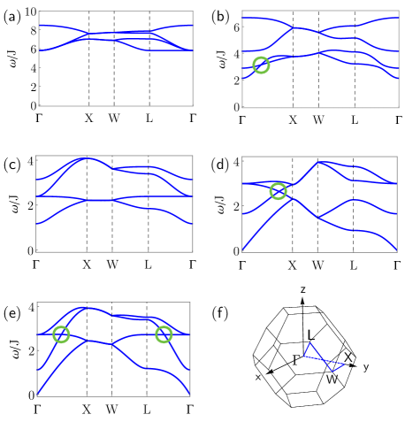
Figure 7: Spin wave excitations of the ordered phases. The parameters are (a) ${D=-J,D_{z}=0}$ (all-in all-out); (b) ${D=J,D_{z}=-0.3J}$ (splayed FM); (c) ${D=-0.3J,D_{z}=0.6J}$ (coplanar XY AFM₁); (d) ${D=0.1J,D_{z}=J}$ (non-coplanar XY AFM); (e) ${D=0.5J,D_{z}=0.1J}$ (coplanar XY AFM₂). In (f) we plot the Brillouin zone of the pyrochlore lattice and label the high symmetry points.

In Fig. 7, we plot the spin wave excitation of each ordered phase along high symmetry lines in Brillouin zone. As expected, the spectra in Fig. 7(a)(b)(c) are fully gapped while in Fig. 7(d)(e), there are gapless pseudo-Goldstone modes at $\Gamma$, reflecting the continuous $U(1)$ degeneracy in the mean-field ground state manifold. Since the degeneracy is accidental, a small gap is expected when we go beyond the linear spin wave approximation.

We further explore the topological spin wave modes in the spectrum. Besides the Weyl nodes (see Fig. 8), we find extra doubly degenerate band touchings, labeled by green circles. These touchings belong to certain nodal lines (see Fig. 8). Since these magnon excitations are bosonic, they occur at the finite energies. These topological magnons Li et al. (2016); Mook et al. (2016); Li et al. (2017a); Owerre (2017a, b); Fransson et al. (2016); Li et al. (2017b) are magnetic analogues of the the electronic topological semimetals Wan et al. (2011); Burkov et al. (2011).

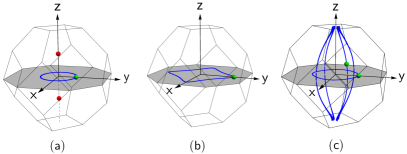
Figure 8: The nodal lines and Weyl nodes of the spin wave excitation. (a) For the same parameters as in Fig. 7(b), there is a nodal contour in the (001) plane (gray) of the reciprocal space. The band touching showed in Fig. 7(b) is labeled by a green dot here. Moreover, there exists a pair of isolated Weyl nodes along $z$ axis, labeled by red dots. (b) For the same parameters as in Fig. 7(d), there is a nodal line in the (001) plane (gray) of the reciprocal space too. Again the band touching showed in Fig. 7(d) is labeled by a green dot. (c) For the same parameters as in Fig. 7(e), the nodal lines form a cage-like structure. One nodal contour is located in the (001) plane (gray) and intersects with the other four nodal lines, of which two are located in the (110) plane and the other two are located in the (1$\bar{1}$0) plane. The two band touchings showed in Fig. 7(e) are labeled by green dots.

V Discussion

V.1 Summary of theoretical results

In this paper, we have proposed a generic spin model to describe the interacting spin-one moments on the pyrochlore lattice. We have established a global phase diagram with very rich phases for this model using several different and complementary methods. The magnetic ordered states are understood from both the mean field theory and the instability of the quantum paramagnetic phase. The relations between different phases are further clarified. Both the magnetic structures of the ordered phases and the corresponding elementary excitations are carefully studied. We point out the existence of degenerate and topological excitations. While these results are valid within the approximation that we made, we would like to point out the caveat of our theoretical results. We expect that our results break down when the system approaches the Heisenberg limit. Thus, the phases in the vicinity of the Heisenberg model of Fig. 1 are expected to altered, and more quantum treatment is needed. The ground state for the pyrochlore lattice Heisenberg model is one of the hardest problems in quantum magnetism. The early theoretical attempts provide insights for the classical limit Moessner and Chalker (1998a, b). Due to the extensive classical ground state degeneracy, the quantum fluctuation is deemed to be very strong when the quantum nature of the spins is considered. Moreover, there should be fundamental distinctions between the spin-1/2 and the spin-1 Heisenberg models.

materials	magnetic ions	$\Theta_{\text{CW}}$	magnetic transitions	magnetic structure	refs
NaCaNi2F7	Ni2+($3d^{8}$)	$-129$K	glassy transition at 3.6K	spin glass	Krizan and Cava,2015
Y2Ru2O7	Ru4+($4d^{4}$)	$-1250$K	AFM transition at 76K	canted AFM ${{\boldsymbol{Q}}={\boldsymbol{0}}}$	Kmieć et al.,2006
Tl2Ru2O7	Ru4+($4d^{4}$)	$-956$K	structure transition at 120K	gapped paramagnet	Lee et al.,2006
Eu2Ru2O7	Ru4+($4d^{4}$)	-	Ru order at 118K	Ru order	Perez1 et al.,2013
Pr2Ru2O7	Ru4+($4d^{4}$), Pr3+($4f^{2}$)	$-224$K	Ru AFM order at 162K	Ru AFM order	Tachibanaa,2007; Zouari et al.,2009
Nd2Ru2O7	Ru4+($4d^{4}$), Nd3+($4f^{3}$)	$-168$K	Ru AFM order at 143K	Ru AFM order	Gaultois et al.,2013
Gd2Ru2O7	Ru4+($4d^{4}$), Gd3+($4f^{7}$)	$-10$K	Ru AFM order at 114K	Ru AFM order ${{\boldsymbol{Q}}={\boldsymbol{0}}}$	Gurgul et al.,2007
Tb2Ru2O7	Ru4+($4d^{4}$), Tb3+($4f^{8}$)	$-16$K	Ru AFM order at 110K	Ru AFM order ${{\boldsymbol{Q}}={\boldsymbol{0}}}$	Chang et al.,2010
Dy2Ru2O7	Ru4+($4d^{4}$), Dy3+($4f^{9}$)	$-10$K	Ru AFM order at 100K	Ru AFM order	Xu et al.,2014
Ho2Ru2O7	Ru4+($4d^{4}$), Ho3+($4f^{10}$)	$-4$K	Ru AFM order at 95K	Ru FM order ${{\boldsymbol{Q}}={\boldsymbol{0}}}$	Wiebe et al.,2004; Taira et al.,2002
Er2Ru2O7	Ru4+($4d^{4}$), Er3+($4f^{11}$)	$-16$K	Ru AFM order at 92K	Ru AFM order ${{\boldsymbol{Q}}={\boldsymbol{0}}}$	Gardner and Ehlers,2009; Taira et al.,2003
Yb2Ru2O7	Ru4+($4d^{4}$), Yb3+($4f^{13}$)	-	Ru AFM order at 83K	Ru AFM order	Taira et al.,2002
Y2Mo2O7	Mo4+($4d^{2}$)	$-200$K	Mo spin glass at 22K	Mo spin glass	Keren and Gardner,2001; Thygesen et al.,2017; Silverstein et al.,2014; Dunsiger et al.,1996
Lu2Mo2O7	Mo4+($4d^{2}$)	$-160$K	Mo spin glass at 16K	Mo spin glass	Clark et al.,2014
Tb2Mo2O7	Mo4+($4d^{2}$), Tb3+($4f^{8}$)	$20$K	spin glass at 25K	spin glass	Jiang et al.,2011; Ehlers et al.,2010; Singh et al.,2008

Table 1: A list of candidate spin-one pyrochlore materials. The null entry means that the data is not available.

V.2 Survery of spin-one pyrochlore materials

There have already been several spin-one pyrochlore materials in the literature. We start with from the Ni-based pyrochlore material NaCaNi₂F₇ Krizan and Cava (2015). This material has a $-129$K Curie-Weiss temperature, and no features of spin orderings are observed in the thermodynamic measurement until a spin glassy transition at 3.6K. The spin glassy transition is evidenced by the bifurcation in the magnetic susceptibility between the zero-field-cooled and field-cooled results. The magnetic entropy saturates to $Rln2$ when the temperature is increased to $70$K Krizan and Cava (2015). The highest temperature $70$K in the entropy measurement is probably not too large to exhaust the actual magnetic entropy as the Curie-Weiss temperature is $-129$K. If one takes this entropy result, this magnetic entropy differs from the simple expectation for the spin-1 local moment and indicates a significant easy-axis spin anisotropy that reduces the total magnetic entropy. In this case, based on our phase diagram in Fig. 1, there would be magnetic orders. It is possible that the exchange randomness becomes important at low temperatures and drives the system into a spin glassy state instead. Since the glassy transition occurs at very low temperatures, the spin physics and dynamics at higher temperatures and energy scales are probably less influenced by the exchange randomness. If the current entropy result is not reliable due to the small upper temperature limit, one could extend the entropy measurement further in the temperature to see if one can exhaust the spin-1 magnetic entropy. In any case, to test the relevance of the model Hamiltonian, it can be helpful to measure the spin correlation in the momentum space with neutron scattering and compare with the theoretical results. Since our spin model contains the spin space anisotropy in addition to the momentum space due to the single-ion anisotropy and Dzyaloshinskii-Moriya interaction, it is also quite useful to carry out the polarized neutron scattering measurement on the single-crystalline sample to detect the spin correlation function in the spin space. A very recent neutron scattering experiment was actually implemented on the single crystal sample. The general features of the spin correlation seem to be well captured by the first neighbor Heisenberg model with much weaker further neighbor interactions Plumb et al. (2017).

In fact, there exists a simple and useful recipe to estimate the Dzyaloshinskii-Moriya interaction but not the single-ion spin anisotropy. The effective magnetic moment of the Ni ion in NaCaNi₂F₇ is found to be $3.7\mu_{\text{B}}$ from the susceptibility data from 5K to 300K Krizan and Cava (2015). This deviates from $2.82\mu_{\text{B}}$ for the pure ${S=1}$ moment in the atomic limit, and this deviation is due to the spin-orbit coupling. It is known that the deviation $\Delta g$ of the Landé $g$ factor is related to the Dzyaloshinskii-Moriya interaction Moriya (1960) with ${\Delta g/g\sim|\boldsymbol{D}_{ij}|/J}$. This suggests that the Dzyaloshinskii-Moriya interaction may be up to 20-30% of the Heisenberg exchange in NaCaNi₂F₇. This suggestion seems to be inconsistent with the conclusion that the system is described by the Heisenberg model in Ref. Plumb et al., 2017. If the latter is true, there should be an unknown cancellation mechanism in the exchange paths that suppress the Dzyaloshinskii-Moriya interaction. If the Dzyaloshinskii-Moriya interaction is sizable, its effect would appear in the low-temperature magnetic properties.

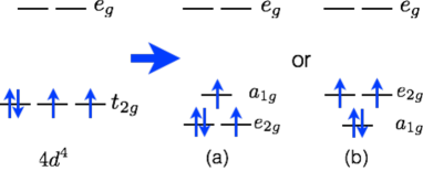
Figure 9: The orbital occupations for $4d^{4}$ electron configuration. Under the trigonal distortion, the three-fold degenerate $t_{2g}$ orbitals are splitted into $a_{1g}$ and two-fold degenerate $e_{2g}$ states. There are two electron occupation configurations here. (a) has an unquenched orbital degree of freedom.

Other existing spin-1 pyrochlore materials are the Ru-based pyrochlore A₂Ru₂O₇ and the Mo-based pyrochlore A₂Mo₂O₇. Both of them are discussed and summarized in a very nice review paper Gardner et al. (2010) by Gardner, Gingras and Greedan. In both systems, the A site can be a rare-earth ion or a non-magnetic ion with no moments. In the former case, the coupling between the rare-earth moments and the Ru/Mo moments may be important, and the rare-earth magnetism also contributes to the magnetic properties of the system. If the Ru-Ru interaction is the dominant one, one may first consider the magnetic physics of the Ru subsystem. In the latter case and also for A=Eu, one only needs to consider the Ru/Mo magnetism.

The Ru⁴⁺ ion has a $4d^{4}$ electron configuration, and the electrons occupy the lower $t_{2g}$ orbitals. Although the atomic spin-orbit coupling is still active due to the partially filled $t_{2g}$ manifold, the Hund’s coupling could suppress the effect of the spin-orbit coupling for the $4d^{4}$ electron configuration. If the spin-orbit coupling is truly dominant over the Hund’s coupling, a quenched local moment would be obtained. Since these are $4d$ electrons, we expect the spin-orbit coupling could just be moderate compared to the Hund’s coupling. From the experimental result of a spin-1 moment for the Ru⁴⁺ ion, it is reasonable to take the view of a moderate spin-orbit coupling. Moreover, as we show in Fig. 9, there can be two different occupation configurations after one includes the trigonal distortion. Fig. 9a has an orbital degeneracy, while Fig. 9b has no orbital degeneracy. The prevailing view of spin-only moment Gardner et al. (2010) for the Ru⁴⁺ ion supports the choice of Fig. 9b. Moreover, due to different orbital occupation configurations and the realization of the spin-orbit coupling for the Ru⁴⁺ ion, although the model stays the same as Eq. (1), the single-ion anisotropy and the Dzyaloshinskii-Moriya interaction would have different relations from the ones in Eqs. (3) and  (4).

As we show in Table 1, almost all materials in the A₂Ru₂O₇ family develop magnetic orders except Tl₂Ru₂O₇. We start from the materials with pure Ru moments. The canted AFM state, that was found for Y₂Ru₂O₇ in Ref. Kmieć et al., 2006, is simply the coplanar AFM₁ state in Fig. 5. It is thus of interest to search for topological magnons in this material. Tl₂Ru₂O₇ experiences a structural transition at 120K that breaks the cubic symmetry, so our model does not really apply here. Eu₂Ru₂O₇ was suggested to develop Ru sublattice orders at 118K and experience a glassy-like transtion at 23K Perez1 et al. (2013). The precise nature of the Ru order is not known.

The Ru materials with the unquenched rare-earth moments contain richer physics than the ones with non-magnetic rare-earth moments. There are three energy scales to consider. From high to low in the energy scales, we would list them as Ru-Ru exchange interaction, $f$-$d$ exchange between the Ru moments and rare-earth moments, and the exchange and dipolar interactions between the rare-earth moments. This hierarchical energy structure arises from the different spatial extension of the $4d$ electrons and the $4f$ electrons. Since the Ru-Ru exchange interaction would be the dominant one, we would expect the Ru moments to develop structures at higher temperatures and influence the rare-earth moments via the $f$-$d$ exchange. The existing experiments support this view Gardner et al. (2010).

The experimental study on these rare-earth based Ru pyrochlores has not been quite systematic yet. Only limited experimental information is available. We here focus the discussion on the systems with more known results. Ho₂Ru₂O₇ was studied using neutron scattering measurements in a nice paper Wiebe et al. (2004) by C.R. Wiebe, et al. The authors revealed the Ru moment order at ${\sim 95}$K and the Ho moment order at ${\sim 1.4}$K. The high temperature Ru magnetic order is consistent with the splayed FM with a splayed angle ${\alpha}\approx 41$ degrees. Under the internal exchange field from the Ru order, the Ho moment further develops a magnetic order at a lower temperature. Despite the agreement between the experimental order and theoretical result, further measurement of the magnetic excitation within the splayed FM can be useful to identify nontrival magnon modes. Ref. Taira et al., 2003 carried out a powder neutron scattering measurement on Er₂Ru₂O₇ and proposed a ${{\boldsymbol{Q}}={\boldsymbol{0}}}$ with a collinear antiferromagnetic magnetic order along ${\langle 001\rangle}$ lattice direction for the Ru moments. Like the Ho₂Ru₂O₇, the Er moments develop a magnetic order at a much lower temperature. Since the Ru moment ordering occurs at much higher temperature and should be understood first. To stabilize the collinear order for the Ru moments, one may need a biquadratic spin interaction Bergman et al. (2006); Penc et al. (2004). This collinear state is actually not among the ordered states that we find. We suscept one ordered state in Fig. 5 may also explain the existing data for Er₂Ru₂O₇. More experiments are needed to sort out the actual magnetic order in this material.

Because the Ru spin-1 moments in these materials often order at a higher temperature, it would be interesting to examine the precise magnetic structure and the magnetic excitations in the future experiments and compare with the theoretical prediction. Future theoretical directions in these systems at least include the understanding of the $f$-$d$ exchange between the rare-earth moments and the Ru moments and the magnetic properties of the rare-earth subsystem. The $f$-$d$ exchange significantly depends on the nature of the rare-earth moment, i.e. whether it is Kramers doublet, non-Kramers doublet or dipole-octupole doublet. As a result, the Ru molecular or internal exchange field on the rare-earth subsystem not only depends on the magnetic structure of the Ru subsystem, but also depends on the form of the $f$-$d$ exchange. This may give rise to rich magnetic structures and properties on the rare-earth subsystems in the ordered phase of the Ru subsystems.

It is interesting to compare the spin-1 Ru pyrochlores with the rare-earth osmates (A₂Os₂O₇) and molybedates (A₂Mo₂O₇). The Os⁴⁺ ion has a $5d^{4}$ electron configuration, and spin-orbit coupling is stronger than Ru⁴⁺. As a result, rather than forming a ${S=1}$ local moment, the magnetic moment of the Os⁴⁺ ion is strongly suppressed by the spin-orbit coupling that would favor a spin-orbital singlet in the strong spin-orbit coupling limit Chen and Balents (2011); Zhao et al. (2016); Khaliullin (2013). Unlike the insulating Ru-based pyrochlores, most Mo-based pyrochlore materials are metallic Gardner et al. (2010). The Mo⁴⁺ has a $4d^{2}$ electron configuration. The metallic behavior is probably because the Hund’s coupling suppresses the correlation effect and induces Hund’s metals Georges et al. (2013). Instead of developing magnetic orders, the insulating ones (Y₂Mo₂O₇, Lu₂Mo₂O₇ and Tb₂Mo₂O₇) all show spin glassy behaviors. The origin of the spin glass in these geometrically frustrated pyrochlore molybedates remains to be a puzzle in the field Gardner et al. (2010). It is possible that, the orbital occupation of the Mo⁴⁺ ion is not given by Fig. 10a and is instead given by Fig. 10b. In that case, the Mo local moment contains a unquenched orbital degree of freedom, and the orbital and spin interact in a Kugel-Khomskii fashion Kugel and Khomskii (1982) and are affected by the lattice phonons. This spin-orbital physics has been suggested for the spinel vanadate AV₂O₄ (A=Ca,Mg,Cd,Zn), where ${V^{3+}:3d^{2}}$ was expected to take the electron configuration in Fig. 10b  Lee et al. (2004); Maitra and Valentí (2007); Giovannetti et al. (2011); Khomskii and Mizokawa (2005); Niitaka et al. (2013); Wheeler et al. (2010) and forms a spin-1 pyrochlore system with additional orbital degree of freedom.

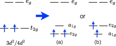
Figure 10: The orbital occupations for $3d^{2}/4d^{2}$ electron configuration. Under the trigonal distortion, the three-fold degenerate $t_{2g}$ orbitals are splitted into $a_{1g}$ and two-fold degenerate $e_{2g}$ states. There are two electron occupation configurations here. (b) has an unquenched orbital degree of freedom.

V.3 Extension to spin-3/2 pyrochlores

Although the major part of the paper deals with the spin-1 pyrochlore materials, the same model actually applies to the spin-3/2 pyrochlore materials. The spin-3/2 moment is a half-integer moment, and the local spin anisotropy acts on it quite differently from the spin-1 moment. Certainly the quantum paramagnetic phase is absent for the spin-3/2 moment, and there are always unquenched local moments regardless of the easy-axis or easy-plane anisotropy. In the strong easy-axis or easy-plane anisotropic limit, the spin-3/2 moment reduces to an effective spin-1/2 moment that can be described by the generic and anisotropic model for the effective spin-1/2 moment. This point of view has been suggested for the Co-based pyrochlore materials NaCaCo₂F₇ and NaSrCo₂F₇ in Ref. Ross et al., 2017. Besides this difference from the spin-1 moment, the magnetic orders, if they occur in the spin-3/2 pyrochlore system, would be similar to the spin-1 pyrochlore system, since the same mean-field Hamiltonian applies to both systems. Moreover, the spin wave excitation would have similar properties. For example, we would expect the existence of the topological spin wave modes such as Weyl magnons in the magnetic excitations of the ordered spin-3/2 pyrochlore materials. In fact, the notion of Weyl magnon was first proposed by our collaborators and us in the context of the Cr-based spin-3/2 breathing pyrochlore systems. The model Hamiltonian, that was used in Ref. Li et al., 2016 did not include the Dzyaloshinskii-Moriya interaction. It was also shown in Ref. Li et al., 2016 that the Weyl magnon is robust against weak perturbation and extends to the regime of a regular pyrochlore system. Besides the Co-pyrochlore and Cr-spinel, the Mn-pyrochlore (A₂Mn₂O₇) is another ideal spin-3/2 system. These materials were studied in the 90s after the discovery of giant magnetoresistance Gardner et al. (2010). Since most of these Mn-pyrochlores are well ordered, it would be exciting to explore the topological magnons in these materials.

VI Acknowledgments

We are indebted to D.-H. Lee and F.-C. Zhang for their advice that wakes me up to write out and/or submit our papers including this one here. We thank T. Senthil for a conversation at the Hong Kong Gordon Research Conference this June about the pyrochlore lattice Heisenberg model on which we shared some common view and have actually expressed in Ref. Chen, 2017b before our conversation. This work is supported by the ministry of science and technology of China with the grant No.2016YFA0301001, the start-up fund and the first-class University construction fund of Fudan University, and the thousand-youth-talent program of China.

Appendix A Dzyaloshinskii-Moriya interaction

Below we list ${\boldsymbol{D}}_{ij}$ vectors in the Dzyaloshinskii-Moriya interaction Elhajal et al. (2005) for bonds in Fig. 2:

$${\boldsymbol{D}}_{01} = \frac{1}{\sqrt{2}}(0,+D,-D),$$ (59)

$${\boldsymbol{D}}_{02} = \frac{1}{\sqrt{2}}(-D,0,+D),$$ (60)

$${\boldsymbol{D}}_{03} = \frac{1}{\sqrt{2}}(+D,-D,0),$$ (61)

$${\boldsymbol{D}}_{12} = \frac{1}{\sqrt{2}}(+D,+D,0),$$ (62)

$${\boldsymbol{D}}_{13} = \frac{1}{\sqrt{2}}(-D,0,-D),$$ (63)

$${\boldsymbol{D}}_{23} = \frac{1}{\sqrt{2}}(0,+D,+D).$$ (64)

Appendix B Transformation of the model

We first define the local coordinate systems where $S^{z}_{i}$ and $S^{\pm}_{i}$ are defined. The choices of the local spin axes are listed in Table 2.

${\mu}$	0	1	2	3
$\hat{x}_{\mu}$	$\frac{1}{\sqrt{6}}[\bar{2}11]$	$\frac{1}{\sqrt{6}}[\bar{2}\bar{1}\bar{1}]$	$\frac{1}{\sqrt{6}}[21\bar{1}]$	$\frac{1}{\sqrt{6}}[2\bar{1}1]$
$\hat{y}_{\mu}$	$\frac{1}{\sqrt{2}}[0\bar{1}1]$	$\frac{1}{\sqrt{2}}[01\bar{1}]$	$\frac{1}{\sqrt{2}}[0\bar{1}\bar{1}]$	$\frac{1}{\sqrt{2}}[011]$
$\hat{z}_{\mu}$	$\frac{1}{\sqrt{3}}[111]$	$\frac{1}{\sqrt{3}}[1\bar{1}\bar{1}]$	$\frac{1}{\sqrt{3}}[\bar{1}1\bar{1}]$	$\frac{1}{\sqrt{3}}[\bar{1}\bar{1}1]$

Table 2: The local coordinate systems for the four sublattices. The same choice can be found for the spin-1/2 Kramers doublet in Ref. Ross et al., 2011.

The relation between the couplings in Eq. (1) and the couplings in Eq. (6) is given as

$$J_{zz} = \frac{1}{3}\left(2\sqrt{2}D-J\right),$$

$$J_{\pm} = -\frac{1}{6}\left(\sqrt{2}D+J\right),$$

$$J_{\pm\pm} = -\frac{1}{3}\left(\frac{D}{\sqrt{2}}-J\right),$$

$$J_{z\pm} = \frac{1}{6}\left(D+2\sqrt{2}J\right).$$ (65)

The bond-dependent phase variables $\gamma_{ij}$ and $\xi_{ij}$ can be written in matrix form as

$$\gamma=-\xi^{*}=\begin{pmatrix}0&1&\text{e}^{i2\pi/3}&\text{e}^{-i2\pi/3}\\ 1&0&\text{e}^{-i2\pi/3}&\text{e}^{i2\pi/3}\\ \text{e}^{i2\pi/3}&\text{e}^{-i2\pi/3}&0&1\\ \text{e}^{-i2\pi/3}&\text{e}^{i2\pi/3}&1&0\end{pmatrix},$$ (66)

where the indices of the matrix label different sublattices.

Appendix C Flavor wave Hamiltonian

The flavor wave Hamiltonian matrix defined in Eq. (14) can be written in block form as

$$M(\boldsymbol{k})=\begin{pmatrix}M_{1}(\boldsymbol{k})&M_{2}(\boldsymbol{k})\\ M_{2}^{*}(\boldsymbol{k})&M_{1}^{*}(\boldsymbol{k})\end{pmatrix},$$ (67)

where $M_{1}(\boldsymbol{k})$ and $M_{2}(\boldsymbol{k})$ are $8\times 8$ matrices and satisfy $M_{1}^{\dagger}(\boldsymbol{k})=M_{1}(\boldsymbol{k})$, $M_{2}^{T}(\boldsymbol{k})=M_{2}(\boldsymbol{k})$.

$M_{1}(\boldsymbol{k})$ and $M_{2}(\boldsymbol{k})$ can be further written in block form as

$$\begin{pmatrix}m_{00}&m_{01}&m_{02}&m_{03}\\ m_{10}&m_{11}&m_{12}&m_{13}\\ m_{20}&m_{21}&m_{22}&m_{23}\\ m_{30}&m_{31}&m_{32}&m_{33}\end{pmatrix},$$ (68)

where $m_{\mu\nu}$s are $2\times 2$ matrices.

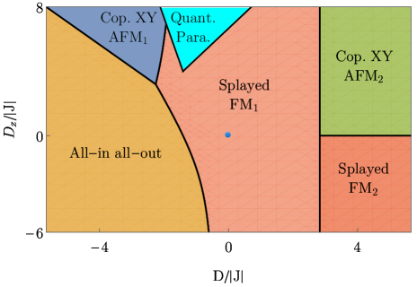
Figure 11: The phase diagram of our generic spin model with ferromagnetic Heisenberg exchange (${J<0}$). The Heisenberg point is labeled by a blue point.

For $M_{1}(\boldsymbol{k})$,

$$m_{\mu\mu} = \frac{1}{2}\begin{pmatrix}D_{z}&0\\ 0&D_{z}\end{pmatrix},$$

$$m_{\mu\nu(\mu\neq\nu)} = 2\cos\Phi_{\mu\nu}\begin{pmatrix}J_{\pm}&J_{\pm\pm}\gamma_{\mu\nu}\\ J_{\pm\pm}\gamma^{*}_{\mu\nu}&J_{\pm}\end{pmatrix}.$$ (69)

For convenience, here and henceforth we define

$$\Phi_{\mu\nu}\equiv\boldsymbol{k}\cdot\left({\boldsymbol{r}_{\mu}}-{\boldsymbol{r}_{\nu}}\right),$$ (70)

where $\boldsymbol{r}_{0}=[000]$, $\boldsymbol{r}_{1}=\frac{1}{4}[011]$, $\boldsymbol{r}_{2}=\frac{1}{4}[101]$, $\boldsymbol{r}_{3}=\frac{1}{4}[110]$.

For $M_{2}(\boldsymbol{k})$,

$$m_{\mu\mu} = \begin{pmatrix}0&0\\ 0&0\end{pmatrix},$$

$$m_{\mu\nu(\mu\neq\nu)} = 2\cos\Phi_{\mu\nu}\begin{pmatrix}J_{\pm\pm}\gamma_{\mu\nu}&J_{\pm}\\ J_{\pm}&J_{\pm\pm}\gamma^{*}_{\mu\nu}\end{pmatrix}.$$ (71)

Appendix D Spin wave Hamiltonian

Figure 12: The parameter regime of the splay angle $\alpha$ in “splayed FM₁” and “splayed FM₂”. For the splayed ferromagnet, the spin on sublattice 0 can be parametrized as $\left({\sin\alpha}/{\sqrt{2}},{\sin\alpha}/{\sqrt{2}},\cos\alpha\right)$, where we set the ferromagnetic component along $z$ direction. In “splayed FM₁” and for fixed $D$, when $D_{z}$ is tuned from negative infinity to positive infinity, the spin on sublattice 0 sweeps from (111) to ($\bar{1}\bar{1}2$) and $\alpha$ takes value from $54.7^{\circ}$ to $-35.3^{\circ}$. When $\alpha=0$, we have a collinear ferromagnetic state. On the other hand, in “splayed FM₂” and for fixed $D$, the spin on sublattice 0 sweeps from (110) to (111) when $D_{z}$ is tuned away from 0. The splay angle $\alpha$ then takes value from 90^∘ to 54.7^∘. When $\alpha=90^{\circ}$, we have a coplanar state.

The entries of the spin wave Hamiltonian in Eq. (53) are given as

$$A_{\mu\mu}=2\sqrt{2}D+D_{z}+2J,$$

$$A_{\mu\nu(\mu\neq\nu)}=\frac{\cos\Phi_{\mu\nu}}{3}(\sqrt{2}D-2J)\Big{[}1+\cos(2\theta+\phi_{\mu\nu})\Big{]},$$

$$B_{\mu\mu}=\frac{1}{2}D_{z},$$

$$B_{\mu\nu(\mu\neq\nu)}=-\frac{1}{6}\cos\Phi_{\mu\nu}\Big{[}(\sqrt{2}D-2J)\cos(2\theta+\phi_{\mu\nu})$$

$$\quad\quad\quad\quad+i(2D+4\sqrt{2}J)\sin(\theta-\phi_{\mu\nu})-3\sqrt{2}D\Big{]},$$

where the angle variable $\phi_{\mu\nu}$ is given as

$$\phi=\begin{pmatrix}0&0&2\pi/3&-2\pi/3\\ 0&0&-2\pi/3&2\pi/3\\ 2\pi/3&-2\pi/3&0&0\\ -2\pi/3&2\pi/3&0&0\end{pmatrix}.$$ (72)

Appendix E Ferromagnetic phase diagram

In Fig. 11, we show the ferromagnetic phase diagram of our generic spin model defined in Eq. (1). In the phase diagram, “quant para” refers to the quantum paramagnetic phase and the other regions are ordered phases. “All-in all-out”, “coplanar XY AFM₁” and “coplanar XY AFM₂” are the same phases as described in the antiferromagnetic phase diagram of Fig. 1. The splayed ferromagnet is divided into “splayed FM₁” and “splayed FM₂” according to the parameter regime of the splay angle $\alpha$, demonstrated in Fig. 12.

Appendix F Order selection on the phase boundaries

F.0.1 ${D_{z}=\sqrt{2}|D|}$

On the line ${D_{z}=\sqrt{2}|D|}$, one have three sets of the ground states with $U(1)$ degeneracy. Combining the “all-in all-out” configuration and the configuration in Eq. (38), one set of the ground states can be parametrized as

$$\left\{\begin{array}[]{l}{\boldsymbol{m}}_{0}=\cos\varphi~{}\frac{1}{\sqrt{3}}(1,1,1)+\sin\varphi~{}\frac{1}{\sqrt{2}}(1,\bar{1},0),\\[11.38092pt] {\boldsymbol{m}}_{1}=\cos\varphi~{}\frac{1}{\sqrt{3}}(1,\bar{1},\bar{1})+\sin\varphi~{}\frac{1}{\sqrt{2}}(\bar{1},\bar{1},0),\\[11.38092pt] {\boldsymbol{m}}_{2}=\cos\varphi~{}\frac{1}{\sqrt{3}}(\bar{1},1,\bar{1})+\sin\varphi~{}\frac{1}{\sqrt{2}}(1,{1},{0}),\\[11.38092pt] {\boldsymbol{m}}_{3}=\cos\varphi~{}\frac{1}{\sqrt{3}}(\bar{1},\bar{1},1)+\sin\varphi~{}\frac{1}{\sqrt{2}}(\bar{1},{1},0).\end{array}\right.$$ (77)

The other two sets are symmetry equivalent and can be obtained by a three-fold rotation.

For each set of the ground states, the minima of the quantum zero-point energy are realized at ${\varphi=0,\pi}$, so the order by quantum disorder effect selects the “all-in all-out” state, see Fig. 13.

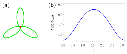
Figure 13: Order by quantum disorder on the line ${D_{z}=\sqrt{2}|D|}$. (a) Three ellipses represent three sets of the ground states with $U(1)$ degeneracy. Their intersection point corresponds to the “all-in all-out” state. (b) For the parametrization in Eq. (77), the minima of the quantum zero-point energy are realized at ${\varphi=0,\pi}$, selecting the “all-in all-out” state (indicated by a red point). The parameters are ${D_{z}=\sqrt{2}|D|=0.5J}$. Here and in Figs. 15, 16, we adopt the Fig. 7 of Ref. Elhajal et al., 2005 to schematically represent the ground state manifold and the order by quantum disorder effect. Note that each state and its time reversal partner are represented by a single point on the ellipses or circles.

F.0.2 ${D=0,D_{z}>0}$

When Dzyaloshinskii-Moriya interaction is switched off, the model describes an anisotropic pyrochlore lattice antiferromagnet. Although the easy-axis anisotropy (${D_{z}<0}$) leads to simple "all-in all-out" configuration in mean-field level, the easy-plane case (${D_{z}>0}$) has a rich structure of the ground state manifold.

First, we have a $U(1)$ ground state manifold defined as

$${\boldsymbol{m}}_{\mu}=\hat{x}_{\mu}\cos\theta+\hat{y}_{\mu}\sin\theta.$$ (78)

For convenience we now dub this manifold “XY₀”. Combining XY₀ and the ground state configurations of “coplanar XY AFM₁”, one can construct extra three sets of generally non-coplanar XY AFM ground states with $U(1)$ degeneracy, dubbed “XY₁”, “XY₂” and “XY₃”, respectively.

We here define the local direction ${\hat{n}_{\mu}^{\phi}\equiv\hat{x}_{\mu}\cos\phi+\hat{y}_{\mu}\sin\phi}$, where $\phi$ is a rotation angle in the local $xy$ plane. The XY₁ ground states are parametrized as

$$\left\{\begin{array}[]{l}{\boldsymbol{m}}_{0}=\cos\varphi~{}\hat{n}_{0}^{{\frac{\pi}{3}}}+\sin\varphi~{}\frac{1}{\sqrt{2}}(1,\bar{1},0),\\[11.38092pt] {\boldsymbol{m}}_{1}=\cos\varphi~{}\hat{n}_{1}^{{\frac{\pi}{3}}}+\sin\varphi~{}\frac{1}{\sqrt{2}}(\bar{1},\bar{1},0),\\[11.38092pt] {\boldsymbol{m}}_{2}=\cos\varphi~{}\hat{n}_{2}^{{\frac{\pi}{3}}}+\sin\varphi~{}\frac{1}{\sqrt{2}}(1,{1},{0}),\\[11.38092pt] {\boldsymbol{m}}_{3}=\cos\varphi~{}\hat{n}_{3}^{{\frac{\pi}{3}}}+\sin\varphi~{}\frac{1}{\sqrt{2}}(\bar{1},{1},0).\end{array}\right.$$ (83)

The symmetry related XY₂ and XY₃ ground states can be obtained by applying the space group symmetry operations.

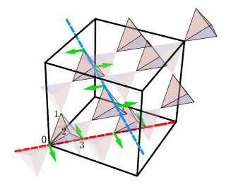
Figure 14: The way to construct ground states with discrete degeneracy. For clarity, we only depict the part of the spin configuration given in Eq. (38) (green arrows). Start from this state, the freedom of simultaneously flipping the spins along any 0-3-0-3-$\cdots$ chain (red dashed line) or 1-2-1-2-$\cdots$ chain (blue dashed line) leads to hugely degenerate ground states.

Moreover, one can construct ground states with huge discrete degeneracy Bramwell (1994). This can be understood like this Bramwell (1994): to optimize the antiferromagnetic Heisenberg interaction, one needs to arrange $\sum_{\mu}{\boldsymbol{m}}_{\mu}=0$ in each tetrahedron, and to satisfy $D_{z}$ term ${\boldsymbol{m}}_{\mu}$, the spins must orient within the local $xy$ plane. Starting from the state defined in Eq. (38) where for this state ${{\boldsymbol{m}}_{0}+{\boldsymbol{m}}_{3}=0}$ and ${{\boldsymbol{m}}_{1}+{\boldsymbol{m}}_{2}=0}$ are satisfied in each tetrahedron and each spin orients within the local $xy$ plane, we can simultaneously flip the spins along any 0-3-0-3-$\cdots$ chain or 1-2-1-2-$\cdots$ chain without changing the mean-field energy (see Fig. 14). Repeating this process, one obtains $4^{N^{2/3}}$ degenerate states where $N$ is the total number of the unit cells. These states are coplanar states in the global $xy$ plane and generally have no translational symmetry. Similar coplanar states in the global $yz$ and $zx$ plane can be readily obtained by applying a three-fold rotation.

Now we discuss the order by quantum disorder effect for the ground state manifold with continuous degeneracy, There is a boundary point ${D_{z}=0.11J}$ separating the “non-coplanar XY AFM” and the “coplanar XY AFM₂” along the ${D=0}$ line, and the order by quantum disorder effect naturally depends on $D_{z}$. For ${D_{z}>0.11J}$, the minima of the quantum zero-point energy select the ground states of “non-coplanar XY AFM” from the continuous manifold, see Fig. 15(a)(b). For ${D_{z}<0.11J}$, the ground states of “coplanar XY AFM₁” and “coplanar XY AFM₂” are selected ground states when quantum fluctuation is included (see Fig. 15(c)(d)).

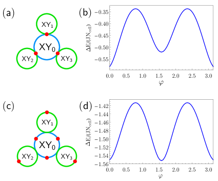
Figure 15: Order by quantum disorder on the line ${D=0,D_{z}>0}$. (a)[(c)], four circles represent four sets of ground states with $U(1)$ degeneracy and the red points indicate the states selected by quantum fluctuation for ${D_{z}>0.11J}$ (${D_{z}<0.11J}$). For the parametrization in Eq.(83), the minima of the quantum zero-point energy are realized at (b) ${\varphi=0,\pi}$ with ${D=0,D_{z}=0.5J}$; (d) $\varphi={\pi}/{2},{3\pi}/{2}$ with ${D=0,D_{z}=0.1J}$.

We mention that all the mean-field ground states found here still hold as ground states for an anisotropic antiferromagnetic Heisenberg model on the breathing pyrochlore lattice, which is previously discussed in Ref. Li et al., 2016.

F.0.3 ${D_{z}=0,D>0}$

When the anisotropy is absent, a negative Dzyaloshinskii-Moriya interaction favors simple “all-in all-out” state, and a positive Dzyaloshinskii-Moriya interaction leads to a ground state manifold with continuous degeneracy. This regime has been studied in the previous work by mean-field theory and classical Monte carlo Elhajal et al. (2005). We here explore the quantum effect beyond the mean-field theory.

Besides the XY₀ manifold, we have another three sets of coplanar ground states in the case of a positive Dzyaloshinskii-Moriya interaction. The “splayed FM” states become coplanar when approaching the limit $D_{z}=0$. One such state is

$$\left\{\begin{array}[]{l}{\boldsymbol{m}}_{0}=\frac{1}{\sqrt{2}}(1,1,0),\\[11.38092pt] {\boldsymbol{m}}_{1}=\frac{1}{\sqrt{2}}(\bar{1},1,0),\\[11.38092pt] {\boldsymbol{m}}_{2}=\frac{1}{\sqrt{2}}(1,\bar{1},0),\\[11.38092pt] {\boldsymbol{m}}_{3}=\frac{1}{\sqrt{2}}(\bar{1},\bar{1},0).\end{array}\right.$$ (88)

Combining this state with proper state in the XY₀ manifold, one can construct a set of coplanar ground states in the global $xy$ plane, parametrized as

$$\left\{\begin{array}[]{l}{\boldsymbol{m}}_{0}=\cos\varphi~{}\hat{n}_{0}^{{-\frac{\pi}{6}}}+\sin\varphi~{}\frac{1}{\sqrt{2}}(1,1,0),\\[11.38092pt] {\boldsymbol{m}}_{1}=\cos\varphi~{}\hat{n}_{1}^{{-\frac{\pi}{6}}}+\sin\varphi~{}\frac{1}{\sqrt{2}}(\bar{1},1,0),\\[11.38092pt] {\boldsymbol{m}}_{2}=\cos\varphi~{}\hat{n}_{2}^{{-\frac{\pi}{6}}}+\sin\varphi~{}\frac{1}{\sqrt{2}}(1,\bar{1},0),\\[11.38092pt] {\boldsymbol{m}}_{3}=\cos\varphi~{}\hat{n}_{3}^{{-\frac{\pi}{6}}}+\sin\varphi~{}\frac{1}{\sqrt{2}}(\bar{1},\bar{1},0).\end{array}\right.$$ (93)

Again the other two sets of coplanar ground states, in the global $yz$ and $zx$ plane respectively, can be obtained by applying the three-fold rotation.

When one includes quantum fluctuation, it turns out that the minima of the quantum zero-point energy select the ground states of “coplanar XY AFM₁” from the whole manifold, see Fig. 16.

The ground state structure of the line ${D_{z}=0,D>0}$ and the order by disorder effect (quantum and thermal) have been extensively studied Elhajal et al. (2005); Canals et al. (2008); Chern (2010). We mention that it is more natural to understand the four-set structure of the ground state manifold by putting this line on the full phase diagram in Fig. 1.

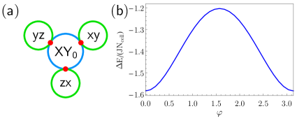
Figure 16: Order by quantum disorder on the line $D_{z}=0,D>0$. (a) Four circles represent four sets of ground states with $U(1)$ degeneracy and the red points indicate the states selected by quantum fluctuation. We refer three sets of coplanar states as “xy”, “yz”, ”zx” respectively. (b) For the parametrization in Eq. 88, the minima of zero-point energy are realized at $\varphi=0,\pi$ with $D_{z}=0,D=0.5J$.

References

- Haldane (1983a) F. D. M. Haldane, Phys. Rev. Lett. 50, 1153 (1983a).
- Haldane (1983b) F. Haldane, Physics Letters A 93, 464 (1983b).
- Affleck et al. (1987) I. Affleck, T. Kennedy, E. H. Lieb, and H. Tasaki, Phys. Rev. Lett. 59, 799 (1987).
- Chen et al. (2011) X. Chen, Z.-C. Gu, and X.-G. Wen, Phys. Rev. B 83, 035107 (2011).
- Wang et al. (2015) C. Wang, A. Nahum, and T. Senthil, Phys. Rev. B 91, 195131 (2015).
- Chen (2017a) G. Chen, Phys. Rev. B 96, 020412 (2017a).
- Savary (2015) L. Savary, ArXiv:1511.01505 (2015).
- Wang et al. (2017) Z. Wang, A. E. Feiguin, W. Zhu, O. A. Starykh, A. V. Chubukov, and C. D. Batista, Phys. Rev. B 96, 184409 (2017).
- Chamorro and McQueen (2017) J. R. Chamorro and T. M. McQueen, arXiv:1701.06674 (2017).
- Cheng et al. (2011) J. G. Cheng, G. Li, L. Balicas, J. S. Zhou, J. B. Goodenough, C. Xu, and H. D. Zhou, Phys. Rev. Lett. 107, 197204 (2011).
- Serbyn et al. (2011) M. Serbyn, T. Senthil, and P. A. Lee, Phys. Rev. B 84, 180403 (2011).
- Bieri et al. (2012) S. Bieri, M. Serbyn, T. Senthil, and P. A. Lee, Phys. Rev. B 86, 224409 (2012).
- Xu et al. (2012) C. Xu, F. Wang, Y. Qi, L. Balents, and M. P. A. Fisher, Phys. Rev. Lett. 108, 087204 (2012).
- Chen et al. (2012) G. Chen, M. Hermele, and L. Radzihovsky, Phys. Rev. Lett. 109, 016402 (2012).
- Hwang et al. (2013) K. Hwang, T. Dodds, S. Bhattacharjee, and Y. B. Kim, Phys. Rev. B 87, 235103 (2013).
- Quilliam et al. (2016) J. A. Quilliam, F. Bert, A. Manseau, C. Darie, C. Guillot-Deudon, C. Payen, C. Baines, A. Amato, and P. Mendels, Phys. Rev. B 93, 214432 (2016).
- Buessen et al. (2017) F. L. Buessen, M. Hering, J. Reuther, and S. Trebst, ArXiv:1706.06299 (2017).
- Gardner et al. (2010) J. S. Gardner, M. J. P. Gingras, and J. E. Greedan, Rev. Mod. Phys. 82, 53 (2010).
- Bramwell and Gingras (2001) S. T. Bramwell and M. J. P. Gingras, Science 294, 1495 (2001).
- Melko et al. (2001) R. G. Melko, B. C. den Hertog, and M. J. P. Gingras, Phys. Rev. Lett. 87, 067203 (2001).
- Castelnovo1 et al. (2008) C. Castelnovo1, R. Moessner, and S. L. Sondhi, Nature 451, 42 (2008).
- Molavian et al. (2007) H. R. Molavian, M. J. P. Gingras, and B. Canals, Phys. Rev. Lett. 98, 157204 (2007).
- Gingras and McClarty (2014) M. J. P. Gingras and P. A. McClarty, Reports on Progress in Physics 77, 056501 (2014).
- Savary and Balents (2016) L. Savary and L. Balents, Reports on Progress in Physics 80, 016502 (2016).
- Onoda and Tanaka (2010) S. Onoda and Y. Tanaka, Phys. Rev. Lett. 105, 047201 (2010).
- Savary and Balents (2012) L. Savary and L. Balents, Phys. Rev. Lett. 108, 037202 (2012).
- Lee et al. (2012) S. Lee, S. Onoda, and L. Balents, Phys. Rev. B 86, 104412 (2012).
- Savary and Balents (2013) L. Savary and L. Balents, Phys. Rev. B 87, 205130 (2013).
- Fukazawa et al. (2002) H. Fukazawa, R. G. Melko, R. Higashinaka, Y. Maeno, and M. J. P. Gingras, Phys. Rev. B 65, 054410 (2002).
- Bramwell et al. (2001) S. T. Bramwell, M. J. Harris, B. C. den Hertog, M. J. P. Gingras, J. S. Gardner, D. F. McMorrow, A. R. Wildes, A. L. Cornelius, J. D. M. Champion, R. G. Melko, and T. Fennell, Phys. Rev. Lett. 87, 047205 (2001).
- Ross et al. (2009) K. A. Ross, J. P. C. Ruff, C. P. Adams, J. S. Gardner, H. A. Dabkowska, Y. Qiu, J. R. D. Copley, and B. D. Gaulin, Phys. Rev. Lett. 103, 227202 (2009).
- Huang et al. (2014) Y.-P. Huang, G. Chen, and M. Hermele, Phys. Rev. Lett. 112, 167203 (2014).
- Chen (2016) G. Chen, Phys. Rev. B 94, 205107 (2016).
- Wan and Tchernyshyov (2012) Y. Wan and O. Tchernyshyov, Phys. Rev. Lett. 108, 247210 (2012).
- Li and Chen (2017) Y.-D. Li and G. Chen, Phys. Rev. B 95, 041106 (2017).
- Yan et al. (2017) H. Yan, O. Benton, L. Jaubert, and N. Shannon, Phys. Rev. B 95, 094422 (2017).
- Savary et al. (2016) L. Savary, X. Wang, H.-Y. Kee, Y. B. Kim, Y. Yu, and G. Chen, Phys. Rev. B 94, 075146 (2016).
- Fennell et al. (2012) T. Fennell, M. Kenzelmann, B. Roessli, M. K. Haas, and R. J. Cava, Phys. Rev. Lett. 109, 017201 (2012).
- Yasui et al. (2002) Y. Yasui, M. Kanada, M. Ito, H. Harashina, M. Sato, H. Okumura, K. Kakurai, and H. Kadowaki, Journal of the Physical Society of Japan 71, 599 (2002).
- Gardner et al. (2001) J. S. Gardner, B. D. Gaulin, A. J. Berlinsky, P. Waldron, S. R. Dunsiger, N. P. Raju, and J. E. Greedan, Phys. Rev. B 64, 224416 (2001).
- Hao et al. (2014) Z. Hao, A. G. R. Day, and M. J. P. Gingras, Phys. Rev. B 90, 214430 (2014).
- Chang et al. (2012) L.-J. Chang, S. Onoda, Y. Su, Y.-J. Kao, K.-D. Tsuei, Y. Yasui, K. Kakurai, and M. R. Lees, Nature Communications 3, 992 (2012).
- Kimura et al. (2013) K. Kimura, K. Nakatsuji, J.-J. Wen, C. Broholm, M. Stone, E. Nishibori, and H. Sawa, Nature Communications 4, 2914 (2013).
- Lhotel et al. (2014) E. Lhotel, S. R. Giblin, M. R. Lees, G. Balakrishnan, L. J. Chang, and Y. Yasui, Phys. Rev. B 89, 224419 (2014).
- Chang et al. (2014) L.-J. Chang, M. R. Lees, I. Watanabe, A. D. Hillier, Y. Yasui, and S. Onoda, Phys. Rev. B 89, 184416 (2014).
- Yasui et al. (2003) Y. Yasui, M. Soda, S. Iikubo, M. Ito, M. Sato, N. Hamaguchi, T. Matsushita, N. Wada, T. Takeuchi, N. Aso, and K. Kakurai, Journal of the Physical Society of Japan 72, 3014 (2003).
- Ross et al. (2011) K. Ross, L. Savary, B. Gaulin, and L. Balents, Phys. Rev. X 1, 021002 (2011).
- Shannon et al. (2012) N. Shannon, O. Sikora, F. Pollmann, K. Penc, and P. Fulde, Phys. Rev. Lett. 108, 067204 (2012).
- Goswami et al. (2016) P. Goswami, B. Roy, and S. Das Sarma, ArXiv:1603.02273 (2016).
- Arpino et al. (2017) K. E. Arpino, B. A. Trump, A. O. Scheie, T. M. McQueen, and S. M. Koohpayeh, Phys. Rev. B 95, 094407 (2017).
- Wen et al. (2017) J.-J. Wen, S. M. Koohpayeh, K. A. Ross, B. A. Trump, T. M. McQueen, K. Kimura, S. Nakatsuji, Y. Qiu, D. M. Pajerowski, J. R. D. Copley, and C. L. Broholm, Phys. Rev. Lett. 118, 107206 (2017).
- MacLaughlin et al. (2015) D. E. MacLaughlin, O. O. Bernal, L. Shu, J. Ishikawa, Y. Matsumoto, J.-J. Wen, M. Mourigal, C. Stock, G. Ehlers, C. L. Broholm, Y. Machida, K. Kimura, S. Nakatsuji, Y. Shimura, and T. Sakakibara, Phys. Rev. B 92, 054432 (2015).
- Chen et al. (2014) G. Chen, H.-Y. Kee, and Y. B. Kim, Phys. Rev. Lett. 113, 197202 (2014).
- Fu et al. (2017) J. Fu, J. G. Rau, M. J. Gingras, and N. B. Perkins, arXiv preprint arXiv:1703.03836 (2017).
- Benton et al. (2012) O. Benton, O. Sikora, and N. Shannon, Phys. Rev. B 86, 075154 (2012).
- Jaubert et al. (2015) L. D. C. Jaubert, O. Benton, J. G. Rau, J. Oitmaa, R. R. P. Singh, N. Shannon, and M. J. P. Gingras, Phys. Rev. Lett. 115, 267208 (2015).
- Applegate et al. (2012) R. Applegate, N. R. Hayre, R. R. P. Singh, T. Lin, A. G. R. Day, and M. J. P. Gingras, Phys. Rev. Lett. 109, 097205 (2012).
- Dunsiger et al. (2011) S. R. Dunsiger, A. A. Aczel, C. Arguello, H. Dabkowska, A. Dabkowski, M.-H. Du, T. Goko, B. Javanparast, T. Lin, F. L. Ning, H. M. L. Noad, D. J. Singh, T. J. Williams, Y. J. Uemura, M. J. P. Gingras, and G. M. Luke, Phys. Rev. Lett. 107, 207207 (2011).
- Sibille et al. (2015) R. Sibille, E. Lhotel, V. Pomjakushin, C. Baines, T. Fennell, and M. Kenzelmann, Phys. Rev. Lett. 115, 097202 (2015).
- Taillefumier et al. (2017) M. Taillefumier, O. Benton, H. Yan, L. Jaubert, and N. Shannon, ArXiv:1705.00148 (2017).
- Chen (2017b) G. Chen, Phys. Rev. B 96, 085136 (2017b).
- Savary and Balents (2017) L. Savary and L. Balents, Phys. Rev. Lett. 118, 087203 (2017).
- Chen (2017c) G. Chen, Phys. Rev. B 96, 195127 (2017c).
- Curnoe (2008) S. H. Curnoe, Phys. Rev. B 78, 094418 (2008).
- Onoda (2011) S. Onoda, Journal of Physics: Conference Series 320, 012065 (2011).
- Krizan and Cava (2015) J. W. Krizan and R. J. Cava, Phys. Rev. B 92, 014406 (2015).
- Krizan and Cava (2014) J. W. Krizan and R. J. Cava, Phys. Rev. B 89, 214401 (2014).
- Ross et al. (2017) K. A. Ross, J. M. Brown, R. J. Cava, J. W. Krizan, S. E. Nagler, J. A. Rodriguez-Rivera, and M. B. Stone, Phys. Rev. B 95, 144414 (2017).
- Sanders et al. (2017) M. B. Sanders, J. W. Krizan, K. W. Plumb, T. M. McQueen, and R. J. Cava, Journal of Physics: Condensed Matter 29, 045801 (2017).
- Witczak-Krempa et al. (2014) W. Witczak-Krempa, G. Chen, Y. B. Kim, and L. Balents, Annual Review of Condensed Matter Physics 5, 57 (2014).
- Elhajal et al. (2005) M. Elhajal, B. Canals, R. Sunyer, and C. Lacroix, Phys. Rev. B 71, 094420 (2005).
- Maekawa et al. (2004) S. Maekawa, T. Tohyama, S. Barnes, S. Ishihara, W. Koshibae, and G. Khaliullin, Physics of Transition Metal Oxides (Springer, 2004).
- Moriya (1960) T. Moriya, Phys. Rev. 120, 91 (1960).
- Joshi et al. (1999) A. Joshi, M. Ma, F. Mila, D. N. Shi, and F. C. Zhang, Phys. Rev. B 60, 6584 (1999).
- Li et al. (1998) Y. Q. Li, M. Ma, D. N. Shi, and F. C. Zhang, Phys. Rev. Lett. 81, 3527 (1998).
- Bradlyn et al. (2016) B. Bradlyn, J. Cano, Z. Wang, M. G. Vergniory, C. Felser, R. J. Cava, and B. A. Bernevig, Science 353 (2016).
- Weng et al. (2016) H. Weng, C. Fang, Z. Fang, and X. Dai, Phys. Rev. B 93, 241202 (2016).
- Zhu et al. (2016) Z. Zhu, G. W. Winkler, Q. Wu, J. Li, and A. A. Soluyanov, Phys. Rev. X 6, 031003 (2016).
- Lv et al. (2017) B. Q. Lv, Z. L. Feng, Q. N. Xu, X. Gao, J. Z. Ma, L. Y. Kong, P. Richard, Y. B. Huang, V. N. Strocov, C. Fang, H. M. Weng, Y. G. Shi, T. Qian, and H. Ding, Nature , 627 (2017).
- Yaouanc et al. (2013) A. Yaouanc, P. Dalmas de Réotier, P. Bonville, J. A. Hodges, V. Glazkov, L. Keller, V. Sikolenko, M. Bartkowiak, A. Amato, C. Baines, P. J. C. King, P. C. M. Gubbens, and A. Forget, Phys. Rev. Lett. 110, 127207 (2013).
- Thompson et al. (2017) J. D. Thompson, P. A. McClarty, D. Prabhakaran, I. Cabrera, T. Guidi, and R. Coldea, Phys. Rev. Lett. 119, 057203 (2017).
- Savary et al. (2012) L. Savary, K. A. Ross, B. D. Gaulin, J. P. C. Ruff, and L. Balents, Phys. Rev. Lett. 109, 167201 (2012).
- Zhitomirsky et al. (2012) M. E. Zhitomirsky, M. V. Gvozdikova, P. C. W. Holdsworth, and R. Moessner, Phys. Rev. Lett. 109, 077204 (2012).
- Zhitomirsky et al. (2014) M. E. Zhitomirsky, P. C. W. Holdsworth, and R. Moessner, Phys. Rev. B 89, 140403 (2014).
- Li et al. (2016) F.-Y. Li, Y.-D. Li, Y. B. Kim, L. Balents, Y. Yu, and G. Chen, Nature Communications 7, 12691 (2016).
- Mook et al. (2016) A. Mook, J. Henk, and I. Mertig, Phys. Rev. Lett. 117, 157204 (2016).
- Li et al. (2017a) F.-Y. Li, Y.-D. Li, Y. Yu, A. Paramekanti, and G. Chen, Phys. Rev. B 95, 085132 (2017a).
- Owerre (2017a) S. A. Owerre, Journal of Physics Communications 1, 025007 (2017a).
- Owerre (2017b) S. A. Owerre, EPL (Europhysics Letters) 117, 37006 (2017b).
- Fransson et al. (2016) J. Fransson, A. M. Black-Schaffer, and A. V. Balatsky, Phys. Rev. B 94, 075401 (2016).
- Li et al. (2017b) K. Li, C. Li, J. Hu, Y. Li, and C. Fang, ArXiv:1703.08545 (2017b).
- Wan et al. (2011) X. Wan, A. M. Turner, A. Vishwanath, and S. Y. Savrasov, Phys. Rev. B 83, 205101 (2011).
- Burkov et al. (2011) A. A. Burkov, M. D. Hook, and L. Balents, Phys. Rev. B 84, 235126 (2011).
- Moessner and Chalker (1998a) R. Moessner and J. T. Chalker, Phys. Rev. B 58, 12049 (1998a).
- Moessner and Chalker (1998b) R. Moessner and J. T. Chalker, Phys. Rev. Lett. 80, 2929 (1998b).
- Kmieć et al. (2006) R. Kmieć, i. d. Z. Świątkowska, J. Gurgul, M. Rams, A. Zarzycki, and K. Tomala, Phys. Rev. B 74, 104425 (2006).
- Lee et al. (2006) S. Lee, J.-G. Park, D. T. Adroja, D. Khomskii, S. Streltsov, K. A. McEwen, H. Sakai, K. Yoshimura, V. I. Anisimov, D. Mori, R. Kanno, and R. Ibberson, Nature Materials 5, 471 (2006).
- Perez1 et al. (2013) S. M. Perez1, R. Cobas, J. M. Cadogan, J. A. Aguiar, C. Frontera, T. Puig, G. Long, M. DeMarco, D. Coffey, and X. Obradors, Journal of Applied Physics 113, 17E102 (2013).
- Tachibanaa (2007) M. Tachibanaa, Journal of Applied Physics 101, 09D502 (2007).
- Zouari et al. (2009) S. Zouari, R. Ballou, A. Cheikhrouhou, and P. Strobel, Journal of Alloys and Compounds 476, 43 (2009).
- Gaultois et al. (2013) M. W. Gaultois, P. T. Barton, C. S. Birkel, L. M. Misch, E. E. Rodriguez, G. D. Stucky, and R. Seshadri, Journal of Physics: Condensed Matter 25, 186004 (2013).
- Gurgul et al. (2007) J. Gurgul, M. Rams, i. d. Z. Świątkowska, R. Kmieć, and K. Tomala, Phys. Rev. B 75, 064426 (2007).
- Chang et al. (2010) L. J. Chang, M. Prager, J. Perbon, J. Walter, E. Jansen, Y. Y. Chen, and J. S. Gardner, Journal of Physics: Condensed Matter 22, 076003 (2010).
- Xu et al. (2014) Z.-C. Xu, M.-F. Liu, L. Lin, H. Liu, Z.-B. Yan, and J.-M. Liu, Front. Phys 9, 82 (2014).
- Wiebe et al. (2004) C. R. Wiebe, J. S. Gardner, S.-J. Kim, G. M. Luke, A. S. Wills, B. D. Gaulin, J. E. Greedan, I. Swainson, Y. Qiu, and C. Y. Jones, Phys. Rev. Lett. 93, 076403 (2004).
- Taira et al. (2002) N. Taira, M. Wakeshima, and Y. Hinatsu, J. Mater. Chem. 12, 1475 (2002).
- Gardner and Ehlers (2009) J. S. Gardner and G. Ehlers, Journal of Physics: Condensed Matter 21, 436004 (2009).
- Taira et al. (2003) N. Taira, M. Wakeshima, Y. Hinatsu, A. Tobo, and K. Ohoyama, Journal of Solid State Chemistry 176, 165 (2003).
- Keren and Gardner (2001) A. Keren and J. S. Gardner, Phys. Rev. Lett. 87, 177201 (2001).
- Thygesen et al. (2017) P. M. M. Thygesen, J. A. M. Paddison, R. Zhang, K. A. Beyer, K. W. Chapman, H. Y. Playford, M. G. Tucker, D. A. Keen, M. A. Hayward, and A. L. Goodwin, Phys. Rev. Lett. 118, 067201 (2017).
- Silverstein et al. (2014) H. J. Silverstein, K. Fritsch, F. Flicker, A. M. Hallas, J. S. Gardner, Y. Qiu, G. Ehlers, A. T. Savici, Z. Yamani, K. A. Ross, B. D. Gaulin, M. J. P. Gingras, J. A. M. Paddison, K. Foyevtsova, R. Valenti, F. Hawthorne, C. R. Wiebe, and H. D. Zhou, Phys. Rev. B 89, 054433 (2014).
- Dunsiger et al. (1996) S. R. Dunsiger, R. F. Kiefl, K. H. Chow, B. D. Gaulin, M. J. P. Gingras, J. E. Greedan, A. Keren, K. Kojima, G. M. Luke, W. A. MacFarlane, N. P. Raju, J. E. Sonier, Y. J. Uemura, and W. D. Wu, Phys. Rev. B 54, 9019 (1996).
- Clark et al. (2014) L. Clark, G. J. Nilsen, E. Kermarrec, G. Ehlers, K. S. Knight, A. Harrison, J. P. Attfield, and B. D. Gaulin, Phys. Rev. Lett. 113, 117201 (2014).
- Jiang et al. (2011) Y. Jiang, A. Huq, C. H. Booth, G. Ehlers, J. E. Greedan, and J. S. Gardner, Journal of Physics: Condensed Matter 23, 164214 (2011).
- Ehlers et al. (2010) G. Ehlers, J. E. Greedan, J. R. Stewart, K. C. Rule, P. Fouquet, A. L. Cornelius, C. Adriano, P. G. Pagliuso, Y. Qiu, and J. S. Gardner, Phys. Rev. B 81, 224405 (2010).
- Singh et al. (2008) D. K. Singh, J. S. Helton, S. Chu, T. H. Han, C. J. Bonnoit, S. Chang, H. J. Kang, J. W. Lynn, and Y. S. Lee, Phys. Rev. B 78, 220405 (2008).
- Plumb et al. (2017) K. W. Plumb, H. J. Changlani, A. Scheie, S. Zhang, J. W. Krizan, J. A. Rodriguez-Rivera, Y. Qiu, B. Winn, R. J. Cava, and C. L. Broholm, arXiv:1711.07509 (2017).
- Bergman et al. (2006) D. L. Bergman, R. Shindou, G. A. Fiete, and L. Balents, Phys. Rev. B 74, 134409 (2006).
- Penc et al. (2004) K. Penc, N. Shannon, and H. Shiba, Phys. Rev. Lett. 93, 197203 (2004).
- Chen and Balents (2011) G. Chen and L. Balents, Phys. Rev. B 84, 094420 (2011).
- Zhao et al. (2016) Z. Y. Zhao, S. Calder, A. A. Aczel, M. A. McGuire, B. C. Sales, D. G. Mandrus, G. Chen, N. Trivedi, H. D. Zhou, and J.-Q. Yan, Phys. Rev. B 93, 134426 (2016).
- Khaliullin (2013) G. Khaliullin, Phys. Rev. Lett. 111, 197201 (2013).
- Georges et al. (2013) A. Georges, L. de’ Medici, and J. Mravlje, Annual Review of Condensed Matter Physics 4, 137 (2013).
- Kugel and Khomskii (1982) K. I. Kugel and D. I. Khomskii, Sov. Phys. Usp. 25, 231 (1982).
- Lee et al. (2004) S.-H. Lee, D. Louca, H. Ueda, S. Park, T. J. Sato, M. Isobe, Y. Ueda, S. Rosenkranz, P. Zschack, J. Íñiguez, Y. Qiu, and R. Osborn, Phys. Rev. Lett. 93, 156407 (2004).
- Maitra and Valentí (2007) T. Maitra and R. Valentí, Phys. Rev. Lett. 99, 126401 (2007).
- Giovannetti et al. (2011) G. Giovannetti, A. Stroppa, S. Picozzi, D. Baldomir, V. Pardo, S. Blanco-Canosa, F. Rivadulla, S. Jodlauk, D. Niermann, J. Rohrkamp, T. Lorenz, S. Streltsov, D. I. Khomskii, and J. Hemberger, Phys. Rev. B 83, 060402 (2011).
- Khomskii and Mizokawa (2005) D. I. Khomskii and T. Mizokawa, Phys. Rev. Lett. 94, 156402 (2005).
- Niitaka et al. (2013) S. Niitaka, H. Ohsumi, K. Sugimoto, S. Lee, Y. Oshima, K. Kato, D. Hashizume, T. Arima, M. Takata, and H. Takagi, Phys. Rev. Lett. 111, 267201 (2013).
- Wheeler et al. (2010) E. M. Wheeler, B. Lake, A. T. M. N. Islam, M. Reehuis, P. Steffens, T. Guidi, and A. H. Hill, Phys. Rev. B 82, 140406 (2010).
- Bramwell (1994) S. T. Bramwell, Journal of Applied Physics 75, 5523 (1994).
- Canals et al. (2008) B. Canals, M. Elhajal, and C. Lacroix, Phys. Rev. B 78, 214431 (2008).
- Chern (2010) G.-W. Chern, arXiv:1008.3038 (2010).