On More Sensitive Periodogram Statistics

Abstract

Period searches in event data have traditionally used the Rayleigh statistic, $R^{2}$. For X-ray pulsars, the standard has been the $Z^{2}$ statistic, which sums over more than one harmonic. For $\gamma$-rays, the $H$-test, which optimizes the number of harmonics to sum, is often used. These periodograms all suffer from the same problem, namely artifacts caused by correlations in the Fourier components that arise from testing frequencies with a non-integer number of cycles. This article addresses this problem. The modified Rayleigh statistic is discussed, its generalization to any harmonic, $\mathcal{R}^{2}_{k}$, is formulated, and from the latter, the modified $Z^{2}$ statistic, $\mathcal{Z}^{2}$, is constructed. Versions of these statistics for binned data and point measurements are derived, and it is shown that the variance in the uncertainties can have an important influence on the periodogram. It is shown how to combine the information about the signal frequency from the different harmonics to estimate its value with maximum accuracy. The methods are applied to an XMM-Newton observation of the Crab pulsar for which a decomposition of the pulse profile is presented, and shows that most of the power is in the second, third, and fifth harmonics. Statistical detection power of the $\mathcal{R}^{2}_{k}$ statistic is superior to the FFT and equivalent to the Lomb–Scargle (LS). Response to gaps in the data is assessed, and it is shown that the LS does not protect against the distortions they cause. The main conclusion of this work is that the classical $R^{2}$ and $Z^{2}$ should be replaced by $\mathcal{R}^{2}_{k}$ and $\mathcal{Z}^{2}$ in all applications with event data, and the LS should be replaced by the $\mathcal{R}^{2}_{k}$ when the uncertainty varies from one point measurement to another.

I. Introduction

The power spectrum refers to the power spectral density distribution of a physical process, whereas the periodogram refers to an estimate of the power spectrum. The most common choice of a periodogram statistic is the Discrete Fourier Transform, and it is generally used in the form of a computationally fast algorithm called Fast Fourier Transform (FFT; see Press et al., 2002) that can only be applied to grouped data.

More sensitive periodogram statistics include the Rayleigh or $R^{2}$-test (Leahy et al., 1983b), the $Z^{2}$-test (Buccheri et al., 1983), and the $H$-test (de Jager et al., 1989, which automatically picks the optimal number of harmonics from which to compute $Z^{2}$). Two important features that make these tests more powerful than the standard FFT periodogram are: (1) they can be applied directly to event arrival times, and thus access all variability timescales present in the data, and (2) they impose no constraints on the frequencies that can be tested, and are thus said to oversample the periodogram by testing timescales other than those corresponding to independent frequencies with an integer number of cycles.

However, oversampling without taking into account the fact that the variables computed to estimate the power at each frequency are correlated within each independent Fourier spacing (IFS) leads to frequency-dependent artifacts that distort the periodogram and in some cases can be mistaken for, and interpreted as, the signature of a coherent periodic modulation. Each of the above-mentioned statistics—the $R^{2}$, $Z^{2}$ and $H$-test—suffers from this.

Although it is powerful—the most powerful according to Leahy et al. (1983b)—in detecting sinusoidal modulations in event data, the Rayleigh statistic achieves this by estimating the power using the fundamental harmonic only. This advantage in regards to strictly sinusoidal signals is a limitation when trying to detect, identify, or study non-sinusoidal pulse shapes. The $Z^{2}$ statistic was devised for this purpose as a generalization of the $R^{2}$ statistic that combines the power estimates from an arbitrary number of harmonics. Even if it is generally true, although not always the case, that the fundamental harmonic carries the bulk of the power, being able to access the additional power contained in higher harmonics confers the $Z^{2}$ statistic an important advantage over the $R^{2}$ statistic, and explains why it is the statistic of choice for event data where pulses are peaked or irregular in shape, as is often the case in pulsars.

A powerful and reliable periodogram statistic must fulfill three conditions: it must (1) be able to use event arrival times in order to access all variability timescales, (2) allow for oversampling in order to explore frequency space without restrictions, and (3) take into account the oscillation in the mean, variance, and covariance of the Fourier components as a function of frequency. These criteria are met by the little known modified Rayleigh statistic discussed in Section IV.

In light of these considerations, we introduce two new periodogram statistics: the generalized ($k$th order) modified Rayleigh statistic, labeled $\mathcal{R}^{2}_{k}$; and the modified $Z^{2}$ statistic, labeled $\mathcal{Z}^{2}$. Because these benefit from all the features of their predecessors but do not suffer from the artifacts caused by unaccounted for correlations in the trigonometric moments, it is probably most sensible to always use the $\mathcal{R}^{2}_{k}$ and $\mathcal{Z}^{2}$ instead of the $R^{2}$ and $Z^{2}$.

Just as the use of the $Z^{2}$ statistic can (and did) replace that of the $R^{2}$ in most applications, the new $\mathcal{Z}^{2}$ statistic should now be used in its stead in all event data applications, whether one is using solely the fundamental, reducing $Z^{2}$ to $R^{2}$ (as in Romano et al. (2010) who nevertheless cite Buccheri et al. (1983) and not Leahy et al. (1983b)); using the first two (i.e., $\mathcal{Z}^{2}_{2}$ as originally suggested by Buccheri et al. (1983), and often used implicitly without actually specifying how many harmonics are used as in Bozzo et al. (2012)); or using several additional higher harmonics ($\mathcal{Z}^{2}_{10}$, for example, as was suggested by de Jager et al. (1986) and subsequently often used in period searches (e.g., de Rosa et al., 2009)). The $\mathcal{R}^{2}_{k}$ statistic that evaluates the contribution of the $k$th harmonic by computing the periodogram for that component is ideally suited for detailed investigations of non-sinusoidal pulse profiles in which the relative contributions of different harmonics to a complex profile are of interest.

This paper begins with a brief presentation of the standard power spectral estimation by FFT in which general notions relevant to spectral estimation are introduced (Section II). The classical $R^{2}$ and $Z^{2}$ periodograms and their limitations are then presented (Section III) before turning to the consideration of the new $\mathcal{R}^{2}_{k}$ and $\mathcal{Z}^{2}$ statistics (Section IV), which are applied to an X-ray observation of the Crab nebula, whose pulsar emission is characterized by a double, narrow-peaked, and thus highly non-sinusoidal pulse profile (Section V). The paper ends with some additional statistical considerations (Section VI) and a short conclusion (Section VII). The derivation and examination of the $\mathcal{R}^{2}_{k}$ statistic are presented in the Appendix.

II. Power Spectral Estimation by FFT

The FFT is performed on $n$ complex numbers, usually a power of 2, represented as an array of length $2n$ (each complex has a real and an imaginary part), and the operation yields $n$ complex numbers. In the case of a light curve, the count rates per bin are real numbers, and therefore the imaginary parts are all zero. The Fourier transform, $H_{j}$ $\equiv$ $\sum^{n-1}_{k=0}h_{k}e^{2\pi ikj/n}$, is periodic in $j$, with a period $n$, and symmetric about $n/2$. It is computed for $(n+1)$ frequencies ranging from $-f_{c}$ to $f_{c}$, in steps of $\delta\/f$ = $1/T$ = $1/n\delta\/t$. Here $f_{c}$ is the critical (highest) or Nyquist frequency defined as $f_{c}$ $\equiv$ $1/2\delta\/t$ = $n/2T$, and $\delta\/t$ is the bin time of the input data. Letting $j$ vary between 0 and $(n-1)$, we find that $H_{j}$ = $H_{n-j}$. Therefore, the transform yields $n/2$ distinct and meaningful complex numbers: the value of $j$ = 0 corresponds to a frequency of zero and equals zero when the mean is subtracted from the data prior to applying the transform; the value of $j$ = $n/2$ corresponds to both $f_{c}$ and $-f_{c}$; and the values of 1 $\leq$ $j$ $<$ $n/2$ correspond to the positive frequencies.

The periodogram is constructed from the output of the transform by squaring the norm of each complex number and then applying a normalization. Common choices include the Leahy normalization (Leahy et al., 1983a) that places the white noise level at 2, and the fractional variance normalization (Belloni & Hasinger, 1990; Miyamoto et al., 1991), where the integral of the periodogram between two frequencies yields the square of the fractional RMS contribution in that range. The FFT is fast and ideal in many applications.

The duration of the observation determines both the minimum and the step between independent frequencies. The number of IFS in the frequency range [$\nu{{}_{\rm{min}}}:\nu{{}_{\rm{max}}}$] is given by $T{{}_{\rm{obs}}}(\nu{{}_{\rm{max}}}-\nu{{}_{\rm{min}}})$ or equivalently by $T{{}_{\rm{obs}}}(1/P{{}_{\rm{min}}}-1/P{{}_{\rm{max}}})$. This defines all independent frequencies up to the critical (maximum) derived from the sampling interval (bin time). A shorter bin time translates into a higher critical frequency, and thereby extends the sampling to higher frequencies; sampling of low frequencies remains unchanged. In this form, there is no sampling between independent frequencies, and this restricts the ability to detect weak signals.

III. The Classical $R^{2}$ and $Z^{2}$ Statistics

One great strength of the Rayleigh and $Z^{2}$ statistics is that they are computed directly from the time of arrival of events, which allows the estimation of the power spectrum using the distribution in time of these events exactly as detected, no matter how many or how few, without grouping, and without restrictions on which frequencies can be tested. This yields a more sensitive way to detect periodic signals, particularly weak signals, especially if the periodicity happens to be exactly between two independent frequencies.

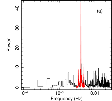
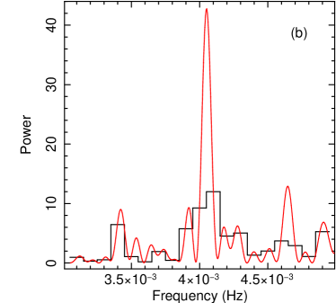
Figure 1.— Using the $R^{2}$ statistic to search for weak periodic signals. The simulated data are of white noise (duration $T$ = 10 ks, mean rate $\mu$ = 0.5 s^-1), with a 10% pulsed fraction (1 of 10 events is modulated; Equation 17) for a sinusoid at 0.00405 Hz ($\approx$ 247 s). The FFT periodogram in black is computed on 512 time bins ($\delta t$=19.531 s) and thus 256 real frequencies with $\nu{{}_{\rm{min}}}$ = $\delta\/f$ = $10^{-4}$ Hz and $\nu{{}_{\rm{max}}}$ = 0.0256 Hz. The Rayleigh periodogram in red is around $\pm$1 IFS of the peak (0.003–0.005 Hz), with sampling of 21 frequencies per IFS. Panel (a) shows the full range, and panel (b) shows the range of the $R^{2}$ periodogram. This example with a period between two independent frequencies was picked to clearly illustrate the important difference in sensitivity that can be achieved in some cases.

The $R^{2}$ statistic uses only the fundamental harmonic, and is therefore most sensitive to sinusoidal signals, but performs quite well for any kind of periodic pulsations. The $Z^{2}$ extends the $R^{2}$ by summing over more than one harmonic, and is therefore more versatile at detecting non-sinusoidal pulse shapes. It also allows, for example, monitoring of the power in the second harmonic in order to study the time evolution of the signal when the power associated with the fundamental is known to fluctuate due to factors unrelated to the signal’s periodic nature (e.g., Burderi et al., 2006).

III.1. The R² Statistic

From a data set comprising $N$ events, the Rayleigh power at a given frequency $\nu$ (or period $P$), is calculated by converting each arrival time, $t_{i}$, to a phase, $\phi_{i}$, given by the fractional part of $2\pi t_{i}\nu$ (or $2\pi t_{i}/P$), and computing

$$R^{2}=\frac{2}{N}\left[\left(\sum_{i=1}^{N}\cos\phi_{i}\right)^{2}+\left(\sum_{i=1}^{N}\sin\phi_{i}\right)^{2}\right].$$ (1)

Figure 1 shows the Rayleigh (red) and FFT (black) periodograms of a simulated white noise with a sinusoidal modulation, showing the full FFT periodogram (panel (a)) and a zoom that highlights the details of the Rayleigh power estimates around the peak (panel (b)). This particular example was picked to illustrate the sometimes remarkable difference in the sensitivity of these two statistics in regards to a weak modulation exactly between two independent frequencies. In the FFT (power of 11.7 at 0.0040 Hz and 9.3 at 0.0041 Hz), for which it is worth noting that it would most probably not have been identified as unusual given the presence of comparable fluctuations in the power throughout the periodogram, compared to the $R^{2}$ in which the signal stands out without a doubt, either about its presence (power of 42.8), its peak location (at 0.004052 Hz), or its low probability of having arisen from a random fluctuation ($10^{-10}$).

III.2. The Z² Statistic

Multiplying the argument of the sine and cosine functions by an integer greater than one when computing $R^{2}$ will probe the data for the contribution from higher order harmonics. Summing over more than one of these yields the $Z^{2}$ statistic, usually labeled $Z^{2}_{m}$ to indicate the number of harmonics $m$ included in the sum:

$$Z^{2}_{m}=\frac{2}{N}\sum_{\rm k=1}^{m}\left[\left(\sum_{i=1}^{N}\cos(k\phi_{i})\right)^{2}+\left(\sum_{i=1}^{N}\sin(k\phi_{i})\right)^{2}\right].$$ (2)

Here also, $N$ is the number of events, and $\phi_{i}$ is the phase of the event with arrival time $t_{i}$, but in addition, we have the integer variables $k$—as the index of the harmonic, and $m$—as the total number of harmonics included in the power estimate.

While the main distinctions between $Z^{2}$ and $R^{2}$ are the former’s sensitivity to non-sinusoidal signals with arbitrary pulse shapes and its ability to look at harmonics beyond the fundamental, another distinction arises from the fact that summing the contribution to the power estimates from more than one harmonic equates to summing as many periodograms as there are harmonics in the sum. Therefore, the sampling distribution of the power estimates—and hence the statistics—depends on this number. Each periodogram has powers that are distributed as a $\chi^{2}_{2}$ variable for white noise. This implies that (for white noise) summing two, three, or four harmonics will yield powers distributed as a $\chi^{2}_{4}$, $\chi^{2}_{6}$, or $\chi^{2}_{8}$ variable. This is a distinction between $R^{2}$ and $Z^{2}_{m}$ that is particularly important when estimating the probability or evaluating the likelihood of a particular value of power in the periodogram. Summing more than one harmonic also decreases the variance because random statistical scatter is averaged over more than one periodogram.

III.3. Artifacts in the R² and Z² Periodograms

Unfortunately, as sensitive as the $R^{2}$ statistic may be to weak sinusoidal signals, and as sensitive as the $Z^{2}$ statistic may be to non-sinusoidal pulse profiles, both suffer in exactly the same way from oversampling artifacts caused by correlations within each IFS throughout the periodogram, but that are most noticeable at lower frequencies (Figure 2, panel (a)).

Figure 2.— Artifacts in the $R^{2}$ periodogram (in red, computed using the same data as in Figure 1) are shown in panel (a) on a truncated linear scale, visibly growing in a power-law fashion toward lower frequencies, with $R^{2}$ estimates between independent frequencies deviating noticeably from the FFT estimates below $\approx 3\times 10^{-3}$ Hz. In panel (b) we see the $\mathcal{R}^{2}_{1}$ statistic applied to the same data, with the periodic signal clearly detected at the same frequency (0.004052 Hz) but at a somewhat lower power from the more accurate calculation (33.1 instead of 42.8, and a probability of $10^{-8}$ instead of $10^{-10}$ of arising from a noise fluctuation).

For independent frequencies (those with an integer number of cycles), the integral of the sine and cosine components is always zero. For all other frequencies, this is not the case, and the value of the integral oscillates between the independent frequencies. This is similarly true for their variances (assumed to be equal to one-half) and covariance (assumed to be zero), all of which also oscillate. As expected, then, powers in the FFT and $R^{2}$ periodograms are equal or nearly so at independent frequencies, but can vary wildly in between.

IV. More Sensitive Periodogram Statistics

Fortunately, because the integral of the Fourier components, as well as their variances and covariance, can be computed exactly, it is possible to account for the fluctuations in their value and thereby eliminate the artifacts that they produce. A modification to the $R^{2}$ statistic that takes into account the expected means and variances (but not the covariance) to standardize the Fourier moments was used (but not emphasized) by de Jager (1994, Equations (8)–(10)) in a search for pulsed emission from $\gamma$-ray pulsars. A full correction that accounts for expected means, variances, and covariance was presented independently by Orford (1996, Section 4.1). The latter’s modified Rayleigh statistic, which we label $\mathcal{R}^{2}$, is much more sensitive than the classical version because it does not suffer from artifacts as does the classical $R^{2}$ statistic. It was formulated for the fundamental harmonic, and this limits its applicability to detailed studies with high-quality data.

IV.1. The new $\mathcal{R}^{2}_{k}$ and $\mathcal{Z}^{2}$ Statistics

We define the generalization of the modified Rayleigh statistic for any harmonic as

$$\mathcal{R}^{2}_{k}=\begin{pmatrix}C_{k}-\langle C_{k}\rangle\\ S_{k}-\langle S_{k}\rangle\end{pmatrix}^{\rm T}\begin{pmatrix}{\sigma^{2}}_{C_{k}}&\sigma_{C_{k}S_{k}}\\ \sigma_{C_{k}S_{k}}&{\sigma^{2}}_{S_{k}}\end{pmatrix}^{-1}\begin{pmatrix}C_{k}-\langle C_{k}\rangle\\ S_{k}-\langle S_{k}\rangle\end{pmatrix}$$ (3)

The dependency on the harmonic is carried by the variable $k$ in the argument of the sine and cosine functions to yield the following expressions for $C_{k}$ and $S_{k}$:

$$C_{k}=\frac{1}{N}\sum_{i=1}^{N}\cos{k\phi_{i}}\hskip 11.38109pt{\rm and}\hskip 11.38109ptS_{k}=\frac{1}{N}\sum_{i=1}^{N}\sin{k\phi_{i}}.$$ (4)

The other terms are defined as follows:

$$\langle C_{k}\rangle = \frac{1}{k\omega\/T}\left[\sin{k\omega\/t}\right]_{t_{1}}^{t_{2}},$$ (5)

$$\langle S_{k}\rangle = \frac{-1}{k\omega\/T}\left[\cos{k\omega\/t}\right]_{t_{1}}^{t_{2}},$$ (6)

$$\sigma^{2}_{C_{k}} = \frac{1}{2N}\left(1+\frac{1}{k\omega\/T}\left[\sin{k\omega\/t}\cos{k\omega\/t}\right]_{t_{1}}^{t_{2}}\right)-\langle C_{k}\rangle^{2},$$ (7)

$$\sigma^{2}_{S_{k}} = \frac{1}{2N}\left(1-\frac{1}{k\omega\/T}\left[\sin{k\omega\/t}\cos{k\omega\/t}\right]_{t_{1}}^{t_{2}}\right)-\langle S_{k}\rangle^{2},$$ (8)

$$\sigma_{C_{k}S_{k}} = \frac{1}{2k\omega\/TN}\left[\sin^{2}k\omega\/t\right]_{t_{1}}^{t_{2}}-\langle C_{k}\rangle\langle S_{k}\rangle.$$ (9)

The terms $\langle C_{k}\rangle$ and $\langle S_{k}\rangle$ are the expectation values, $\sigma^{2}_{C_{k}}$ and $\sigma^{2}_{S_{k}}$ are the variances, and $\sigma_{C_{k}S_{k}}$ is the covariance of $C_{k}$ and $S_{k}$. (See the Appendix for the details of the derivation.)

Figure 2 panel (a) shows the $R^{2}$ periodogram, and panel (b) shows the modified Rayleigh statistic and demonstrates the advantage it has over the standard FFT periodogram for detecting weak signals peaking between independent frequencies without the severely limiting disadvantages of the classical Rayleigh statistic. $\mathcal{R}^{2}_{k}$ is identically as sensitive as $\mathcal{R}^{2}$ for the fundamental harmonic (by mathematical definition), but it is, in addition, equally sensitive for any other harmonic.

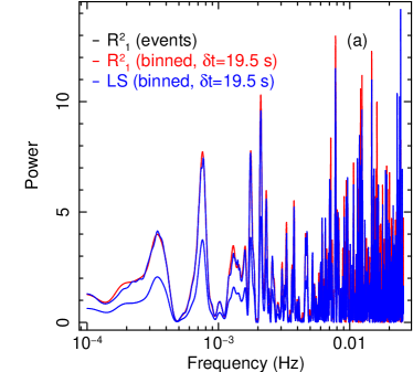
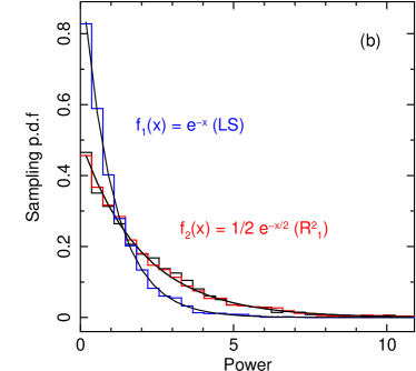
Figure 3.— Comparison in panel (a) of the $\mathcal{R}^{2}_{k}$ statistic for event data (Equation 3, in black) and binned data (Equation 15, in red), with the LS statistic (Equation 16, in blue), showing the corresponding sampling distributions in panel (b), all of which follow the expectation (regardless of the sampling factor).

Because the $Z^{2}$ periodogram is a sum of $R^{2}_{k}$ components, it is therefore natural to use the much more sensitive $\mathcal{R}^{2}_{k}$ as the kernel for a new, modified $Z^{2}$ statistic, $\mathcal{Z}^{2}$, defined as

$$\mathcal{Z}^{2}=\sum\mathcal{R}^{2}_{k}.$$ (10)

Summing as many harmonics as deemed necessary depending on the profile (or expected profile) ensures that all the power present in the selected harmonics of the periodic modulation is included and yields the highest possible peak in the final $\mathcal{Z}^{2}$ periodogram. But because different harmonics will be distributed differently around the peak, they will in general also reach their maxima at slightly different frequencies. Therefore, to derive a single best estimate of the signal’s frequency, we need a way to combine the information carried by each harmonic that maximizes accuracy. For this purpose we construct a weighted mean statistic given by

$$f_{w}=\frac{\sum w_{k}f_{k}}{\sum w_{k}},$$ (11)

where the weight of each term, $w_{k}$, is the ratio of the peak power ($\mathcal{R}^{2}_{k}({\rm peak\/})$) to the square of the peak’s half width at half maximum ($\sigma^{2}_{k}$). The motivation is to give more weight to the value of the peak frequency derived from taller and narrower peaks. The $k$th harmonic is therefore weighted by

$$w_{k}=\frac{\mathcal{R}^{2}_{k}({\rm peak\/})}{\sigma^{2}_{k}}.$$ (12)

The uncertainty on the resulting frequency is calculated using the peak widths of the contributing harmonics:

$$\sigma_{f_{w}}=\frac{1}{\sqrt{\sum\sigma^{2}_{k}}},$$ (13)

where the sum is over the same harmonics as those used in Equation 11 to compute the weighted mean frequency. The use of these is illustrated in Section V.

The periodogram statistics $\mathcal{R}^{2}_{k}$ and $\mathcal{Z}^{2}$ of Equations (3)–(9) and (10)–(13) are formulated for event data and thus cannot be used on binned or point measurement data. We therefore introduce a suitable formulation for such cases.

IV.2. The $\mathcal{R}^{2}_{k}$ for Binned Data and Point Measurements

A great part of the strength of an event data periodogram statistic is that it is computed directly from the event arrival times. This gives us access to the highest frequencies that cannot be investigated when grouping the data on an even slightly longer timescale. Another important feature of the $\mathcal{R}^{2}_{k}$ is that it allows for the testing of as many frequencies as desired without distorting the periodogram (i.e., without distorting the sampling distribution); this is a feature that is essential when searching for weak, low-frequency signals. A version of the $\mathcal{R}^{2}_{k}$ and (by extension) $\mathcal{Z}^{2}$ statistics for binned data or point measurements of an intensity with an associated uncertainty (as in radio data, for example) extends the use of these sensitive periodograms to data other than lists of arrival times.

This is the $\mathcal{R}^{2}_{k}$ statistic for light curves:

$$\mathcal{R}^{2}_{k}=\frac{\left(\sum_{i=1}^{n}\rho_{i}\cos{k\phi_{i}}\right)^{2}}{\sum_{i=1}^{n}(\rho_{i}\cos{k\phi_{i}})^{2}}+\frac{\left(\sum_{i=1}^{n}\rho_{i}\sin{k\phi_{i}}\right)^{2}}{\sum_{i=1}^{n}(\rho_{i}\sin{k\phi_{i}})^{2}}$$ (14)

The sum is performed over $n$—the number of bins in the time series, instead of on $N$—the number of events in the list. The phases, $\phi_{i}$, are calculated using the time of the measurement or the center of the bin, and the $\cos{k\phi_{i}}$ and $\sin{k\phi_{i}}$ terms are weighted by $\rho_{i}=r_{i}/\sigma^{2}_{i}$ defined as the mean-subtracted intensity, $r_{i}$, divided by the square of the uncertainty, $\sigma^{2}_{i}$, for each measurement.

For the simplest case, $k=1$, we get the modified Rayleigh or $\mathcal{R}^{2}_{1}$ statistic for binned data and point measurements:

$$\mathcal{R}^{2}_{1}=\frac{\left(\sum_{i=1}^{n}\rho_{i}\cos\phi_{i}\right)^{2}}{\sum_{i=1}^{n}(\rho_{i}\cos\phi_{i})^{2}}+\frac{\left(\sum_{i=1}^{n}\rho_{i}\sin\phi_{i}\right)^{2}}{\sum_{i=1}^{n}(\rho_{i}\sin\phi_{i})^{2}}$$ (15)

The $\mathcal{R}^{2}_{1}$ for light curves is reminiscent of the Lomb–Scargle (LS) statistic (Scargle, 1982):

$$\mathcal{P}(\omega)=\frac{1}{2\sigma^{2}}\!\!\left[\!\frac{\left(\sum r_{i}\cos\omega(t_{i}-\tau)\right)^{2}}{\sum\cos\omega(t_{i}-\tau)}+\frac{\left(\sum r_{i}\sin\omega(t_{i}-\tau)\right)^{2}}{\sum\sin\omega(t_{i}-\tau)}\right]\qquad$$ (16)

where, as above, all sums on $i$ are from 1 to $n$; $\sigma^{2}$ is the variance of the mean-subtracted rates; $r_{i}$ is the mean-subtracted count rate in bin $i$; $\omega=2\pi/P=2\pi\nu$ is the angular frequency; $t_{i}$ is the time at the bin center; and $\tau$ is defined according to $\tan(2\omega\tau)=\sum_{i=1}^{n}\sin{2\omega t_{i}}/\sum_{i=1}^{n}\cos{2\omega t_{i}}$ (see Press et al., 2002).

As is shown in panel (a) of Figure 3, the periodograms resulting from applying the $\mathcal{R}^{2}_{1}$ or LS statistics to white noise data are virtually identical in shape. The LS differs by a factor of two in normalization that translates into different sampling distributions shown in panel (b): $f(x)$ = $\text@frac{1}{2}\,e^{-x/2}$ for the $\mathcal{R}^{2}_{1}$, and $f(x)$ = $e^{-x}$ for the LS statistic. Another difference is that the popular and commonly used LS periodogram of Equation 16 does not take into account uncertainties (but see Scargle, 1989).

It is important to highlight that the size of the uncertainties, no matter how large this may be, does not affect the shape of the periodogram. It is the variance in the values of uncertainties—the magnitude of the variations between individual uncertainties in the set of measurements—that affects the periodogram. This is illustrated in the Appendix.

V. Multi-harmonic Decomposition of the Crab Pulsar’s X-ray Pulse Profile

The Crab pulsar, with its highly peaked and asymmetric pulse profile, is an excellent example for which it is not only useful but necessary to use several harmonics to characterize the pulse shape and accurately estimate the spin period. We use an XMM-Newton observation to illustrate in practical terms the use of the statistics introduced above for timing studies of pulsars with non-sinusoidal profiles. The $\mathcal{R}^{2}_{k}$ statistic (Equations (3) or (14)) allows us to compute the periodogram for each harmonic individually and thus see each one’s relative contribution to the pulse, and Equations (11)–(13) allow us to most accurately compute the pulse frequency and the uncertainty on its value by combining statistically the information from each of the individual harmonics.

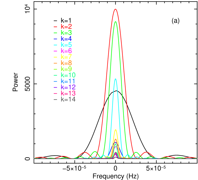
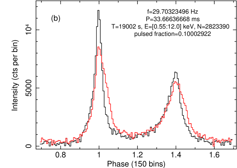
Figure 4.— Multi-harmonic periodogram of the Crab pulsar’s X-ray emission centered on the pulse frequency (a) and phasograms resulting from folding the arrival times on our best estimate of the pulse frequency compared to the frequency derived from the radio ephemerides (b). The data is from an XMM-Newton observation (ID 0611181501-003 on 2012 February 24–25) with an elapsed time of 19,002 s, using the Epic PN Timing/FastBurst data comprising 2823390 events in the range 0.55–12.0 keV (mean rate 148.6 s^-1).

Figure 4 shows (in panel (a)) the multi-harmonic decomposition of the Crab pulsar’s pulse up to $k=14$ where we see that the highest peaks are those of the second, third, and fifth harmonics, and (in panel (b)) the profiles that result from folding the data at our best estimate of the X-ray pulse frequency (in black) from the first five harmonics (details in Table 1), or folding at the frequency derived from the Jodrell Bank ephemerides for the midpoint of the observation (in red).

Table 1Characteristics of the First Five Harmonics

Harmonic	Peak Height	Frequency	HWHM
(k)	($\mathcal{R}^{2}$ Power)	(Hz)	($10^{-6}$ Hz)
1	4537	29.70323424	23.81
2	9988	29.70323534	12.19
3	9155	29.70323486	7.764
4	1097	29.70323461	5.847
5	5342	29.70323499	4.689
1–5${}^{~{}\mathrm{a}}$	30119	29.70323496	3.165

VI. Additional Statistical Considerations

VI.1. Signal Detection with the $\mathcal{R}^{2}$ Statistic

It was shown in Figure 1 that under certain conditions the power at a given frequency can be underestimated to the extent of not being identified as an interesting feature. The performance of a statistic can be evaluated using simulations. We simulate data that contain a signal of specified signal-to-noise ratio ($\rm{S/N}$; Equation 17), and count how often a detection would be claimed given a particular threshold. The statistics are compared on an equal footing because the data are the same. We can estimate the probability of false negatives, $\beta$ (missing the signal that is there: a type II error), often of greater interest when searching for weak signals, as well as the probability of false positives, $\alpha$ (claiming a detection when there is no signal: a type I error). The fraction of false negatives is $1-\hat{\beta}$, and the fraction of false positives is $1-\hat{\alpha}$. The former quantifies the statistic’s sensitivity (how often it detects a signal that is in the data), and the latter quantifies its reliability (how often it detects a signal that is not there).

If the $\rm{S/N}$ of the sinusoidal signal is high, any periodogram will detect the modulation. The considerations herein are therefore of practical relevance only for weak signals, particularly when they are at low frequencies for which the $\mathcal{R}^{2}_{1}$ is best suited. For event data the $\rm{S/N}$ is

$$\rm{S}/\rm{N}=\frac{S}{\sqrt{S+B}}=\frac{\pi\/N}{\sqrt{N}}=\pi\sqrt{N},\\$$ (17)

where $S$ and $B$ respectively stand for the number of signal and background events, $N$ for their sum (the total number of events), and $\pi$ for the pulsed fraction. We consider sinusoids.

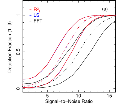
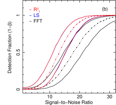
Figure 5.— Detection fraction as a function of $\rm{S/N}$ for a sinusoidal modulation shown in panel (a) for a period of 2857 s (3.5 cycles in 10 ks) in a white noise background, and in panel (b) for a period of 2222 s (4.5 cycles) in red noise with $\alpha=1$. The curves are derived from 10,000 runs for each $\rm{S/N}$ value (marked by dots on the dashed curves). Each run produces a number of background and signal events based on the pulsed fraction, $\pi$ (Equation 17). The average background power is determined in the range $\pm 3$ IFS, and the peak search is done within $\pm 1$ IFS. The thresholds are defined as the likelihood ratios of the normal density at 2.5$\sigma$, 3.0$\sigma$, and 3.5 $\sigma$ with respect to its mode at zero: they are equal to $4.4\times 10^{-2}$, $1.1\times 10^{-2}$, and $2.2\times 10^{-3}$, respectively. The detection fraction is the number of peaks (out of 10,000) with a likelihood ratio equal to or less than the threshold.

Figure 5 shows the results of simulations done to estimate the proportion of false negatives as a function of $\rm{S/N}$ for white and red noise in the limiting case of the lowest detectable frequency for which the period is right between two independent test frequencies. The comparison is between the FFT (black), the LS (blue), and the $\mathcal{R}^{2}_{1}$ periodograms (red), and the results are presented using likelihood intervals between 2.5$\sigma$ (upper) and 3.5$\sigma$ (lower curves), with the dashed lines at 3$\sigma$ (in the Gaussian sense).

The $\mathcal{R}^{2}_{1}$ and LS (scaled by a factor of 2) perform identically well, and significantly better than the FFT. The difference between having a white or red noise background is substantial: for example, a 97% detection fraction at 3$\sigma$ is reached at an $\rm{S/N}$ of 11 for white noise, but at an $\rm{S/N}$ of 21 for red noise. Because we rely on the likelihood ratio to compare against the average background, larger fluctuations in the periodogram caused by the red noise affect detection sensitivity ($1-\hat{\beta}$) but not reliability ($1-\hat{\alpha}$). Calculated in the same way but using background events only, the false detection fraction is very low at around 1.7%, and even more importantly, it is practically the same for white noise as it is for the $\alpha=1$ red noise.

VI.2. Effects of Data Gaps

Gaps in the data introduce structures in the periodogram. To constrain and quantify these effects cannot be done in a general way because they depend on the data and on the size and distribution of gaps within the data. Carrying out a study to investigate gap-induced modifications of the periodogram for any number of gap structures and data sets, real or simulated, could be useful and informative (maybe even essential) depending on the application. But in order to be of practical use, the study would have to be focused on the problem at hand, which would define the parameter space to be explored based on the instrumental and observational features of the telescope, and the physical and statistical characteristics of the source. Here we want to illustrate the effects of gaps for a few simple cases only to get an idea of their magnitude and of the performance of the LS statistic—specifically formulated to handle gaps—compared to the $\mathcal{R}^{2}_{1}$.

​​​​​​
​​​​​​

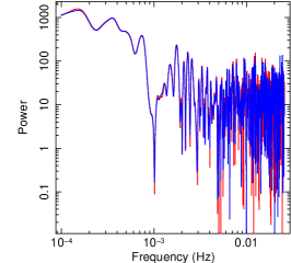
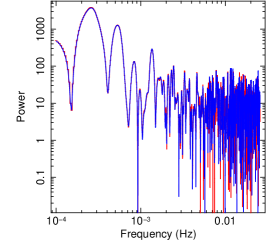
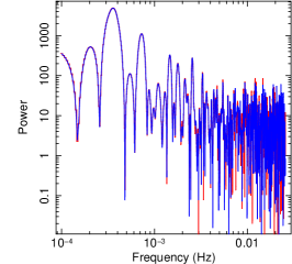
Figure 6.— Illustration of the effects of gaps on the periodogram of the data used in Figure 3. The time series are in the top row, above their respective periodogram. The $\mathcal{R}^{2}_{1}$ statistic is in red and LS in blue. The observation duration is 10 ks, and the gaps of 1 ks in length are equally spaced.

The data are those of Figure 3, and we consider three cases with one, two, and three gaps equally spaced within the observation, removing a progressively larger fraction of the data, from 10% to 30%. Figure 6 shows the time series (top) and their periodograms (bottom; $\mathcal{R}^{2}_{1}$ in red and LS in blue) that have been normalized such that the integrated power (area under the curve) equals one, and plotted on a log–log scale to emphasize the power-law like reddening effect of the gaps. In each case the periodograms are practically indistinguishable in shape. Thus it is seen that both the $\mathcal{R}^{2}_{1}$ and the LS suffer identically from the presence of gaps in the data, and that the latter indeed does not confer any kind of protection against gap-induced distortions of the periodogram as is thought by many to be the case.

VII. Conclusion

Event data periodogram statistics are an important tool for studies of the detailed distribution in time of the detected events without having to group them, and being able to work directly with each event’s recorded arrival time. This is particularly important for X-ray and $\gamma$-ray pulsars. Traditional statistics commonly and currently used for such studies include the Rayleigh or $R^{2}$, $Z^{2}$, and $H$ statistics, the latter two having the former as their kernel. To maximize sensitivity to weak periodic signals, it is essential to test frequencies that are between independent Fourier frequencies. The Rayleigh, and all statistics based on it, allow for this kind of unrestricted sampling of frequency space.

However, because of correlations in the Fourier moments for those frequencies that have a non-integer number of cycles within the observation duration, all these periodograms suffer from distorting artifacts. These distortions severely limit the sensitivity of the statistic to weak signals, especially at lower frequencies.

More sensitive statistics must have a mechanism to take these correlations into account when computing the Fourier power. This is achieved by the modified Rayleigh statistic, $\mathcal{R}^{2}$, the generalization of it for an arbitrary harmonic, $\mathcal{R}^{2}_{k}$, and the sum of more than one of the latter’s components, $\mathcal{Z}^{2}$.

In addition, the new $\mathcal{R}^{2}_{k}$ can be used to decompose a pulse profile by looking at the periodograms for individual harmonics. This is especially useful when some harmonics are better suited to estimate the pulse frequency and study its evolution in time, as is the case for the Crab’s pulsar and most likely several other similarly fast spinning millisecond X-ray pulsars. The new $\mathcal{Z}^{2}$ allows the possibility of summing several individual harmonics to maximize sensitivity to weak signals or to study characteristics that find their expression in certain harmonics more than in others. In the Crab pulsar, for example, most of the power is found in the second, third, and fifth harmonics.

Having access to the information carried by each individual harmonic allows us to combine these statistically to derive the best estimate of the pulse frequency as well as an estimate of the uncertainty on this value. This is done using a weighted sum that takes into account the height and width of each periodogram’s peak around the pulse frequency.

For weak, low-frequency, sinusoidal periodic signals, the more sensitive statistics are the $\mathcal{R}^{2}_{1}$ and LS that outperform the standard FFT peridogram by a factor of about two in the detection fraction at intermediate values of $\rm{S/N}$. This is true for white and red noise. In terms of the detection fraction of false positives, the $\mathcal{R}^{2}_{1}$ and LS perform equally well and retain the same fraction independently of the sampling factor per IFS. Gaps in the data have indistinguishable effects on both. This suggests that in the presence of data gaps, using the LS does not provide a built-in protection as is generally believed, and that careful considerations about the shape of the periodogram may require modeling tailored to the application and data.

The main conclusions of this work are that the classical $R^{2}$ and $Z^{2}$ should be replaced by $\mathcal{R}^{2}_{k}$ and $\mathcal{Z}^{2}$ in all applications with event data because they are far more sensitive to weak signals, and the LS should be replaced by the $\mathcal{R}^{2}_{k}$ for light curves when the uncertainties vary from one point measurement to another because their variance can have important effects on the shape of the periodogram.

Appendix A The $\mathcal{R}^{2}_{k}$ Statistic: Derivation

A.1. Event Data

The classical Rayleigh statistic can be expressed as

$$R^{2}=2N(C^{2}+S^{2}),$$ (A1)

where $C$ and $S$ are defined as:

$$C=\frac{1}{N}\sum_{i=1}^{N}\cos{\phi_{i}}\hskip 11.38109pt{\rm and}\hskip 11.38109ptS=\frac{1}{N}\sum_{i=1}^{N}\sin{\phi_{i}}.$$ (A2)

Assuming that $\phi$ is uniformly distributed, the probability of it having a value between 0 and 2$\pi$ is constant. This implies that its associated PDF, the normalized probability density, is given by $f(\phi)$ = $1/2\pi$.

According to the central limit theorem, the sum of $N$ independent random variables $X_{i}$, each distributed identically about a mean $\mu$ with a finite variance $\sigma^{2}$, is a normal random variable distributed about a mean equal to $N\mu$ with a variance of $N\sigma^{2}$. The distribution of the means $\mu_{i}$ also follows a normal with variance given by $\sigma^{2}/N$.

In the case of the Rayleigh statistic, given that $C$ and $S$ are in fact the expectation values of $\cos{\phi_{i}}$ and $\sin{\phi_{i}}$, respectively, they are therefore distributed as normals about $\langle\cos\phi_{i}\rangle$ and $\langle\sin\phi_{i}\rangle$ with variances of $\sigma^{2}_{C}$ = $Var(\cos{\phi_{i}})/N$ and $\sigma^{2}_{S}$ = $Var(\cos{\phi})/N$.

First, $\langle\cos{\phi}\rangle$ = $\langle\sin{\phi}\rangle$ = 0, since the integrals of $\cos{\phi}$ and $\sin{\phi}$ from 0 to $2\pi$ are both equal to 0; therefore, $\langle C\rangle$ = $\langle S\rangle$ = 0. Second, the variances $Var(\cos{\phi})$ and $Var(\sin{\phi})$ are equal and given by

$$Var(\cos{\phi}) = \langle\cos^{2}{\phi}\rangle-\langle\cos{\phi}\rangle^{2}$$

$$= \int_{0}^{2\pi}f(\phi)\cos^{2}{\phi}\,{\rm d}\phi-0$$

$$= \int_{0}^{2\pi}\frac{1}{2\pi}\cdot\frac{1}{2}(1+\cos{2\phi})\,{\rm d}\phi=\frac{1}{2}.$$

Therefore, $\displaystyle\sigma^{2}_{C}=\sigma^{2}_{S}=1/2N$.

Finally, since $Var(qX)$ = $q^{2}Var(X)$, where $q$ is a constant, the scaled variables $c$ = $\sqrt{2N}\cdot\/C$ and $s$ = $\sqrt{2N}\cdot\/S$, with $Var(\sqrt{2N}\cdot C)=Var(\sqrt{2N}\cdot S)=2N\cdot\sigma^{2}_{C}=1$, are both distributed according to the standard normal. This implies that $R^{2}$ = $c^{2}+s^{2}$ = $2NC^{2}+2NS^{2}$ = $2N(C^{2}+S^{2})$, is the sum of the squares of two normally distributed, zero-mean and unit-variance, independent variables. The square of a standard normal variable is $\chi^{2}_{1}$ distributed, and the sum of $\chi^{2}$ variables is also a $\chi^{2}$ variable for which the number of dof is given by the sum of the dof of the individual variables. Thus, $R^{2}$ is $\chi^{2}_{2}$ distributed.

The frequencies within an IFS are by definition not independent. Therefore, sampling more than one frequency per IFS introduces a correlation in the values of $C$ and those of $S$ within the IFS, and thus also in the power estimates derived from them. To remove these correlations and recover the $\chi^{2}_{2}$ distribution of powers for white noise, we must calculate the expectation values, variances, and covariance directly from the data and incorporate them in the calculation of the power.

The modified Rayleigh statistic is defined as

$$\mathcal{R}^{2}=\begin{pmatrix}{C-\langle C\rangle}\\ {S-\langle S\rangle}\end{pmatrix}^{\rm T}\begin{pmatrix}\sigma^{2}_{C}&\sigma_{CS}\\ \sigma_{CS}&\sigma^{2}_{S}\end{pmatrix}^{-1}\begin{pmatrix}{C-\langle C\rangle}\\ {S-\langle S\rangle}\end{pmatrix}.$$ (A4)

Note that if we replace $\langle C\rangle$ and $\langle S\rangle$ by 0, as is the case when sampling the complete phase between 0 and $2\pi$; $\sigma^{2}_{C}$ and $\sigma^{2}_{S}$ by 1, and $\sigma_{CS}$ by 0, as is the case for independent normal variables, we recover the classical Rayleigh statistic:

$$R^{2}=\begin{pmatrix}c&s\end{pmatrix}\begin{pmatrix}1&0\\ 0&1\end{pmatrix}\begin{pmatrix}c\\ s\end{pmatrix}=c^{2}+s^{2}$$ (A5)

In constructing $\mathcal{R}^{2}$, we must compute $\langle C\rangle$, $\langle S\rangle$, $\sigma_{C}^{2}$, $\sigma_{S}^{2}$, and $\sigma_{CS}$. The integral is over time and not over phase. The duration of the observation is $T$ = $t_{2}-t_{1}$, and $\phi$ is replaced by $\omega\/t$, where $\omega$ = $2\pi\nu$ = $2\pi/p$, $\nu$ is the test frequency and $p$ is the corresponding test period.

​​​​​​​​​

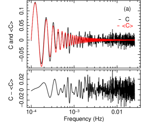
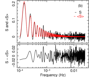
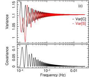
Figure 7.— Components of the $\mathcal{R}^{2}_{1}$ statistic for the data of Figure 3. Panels (a) and (b) show, plotted as a function of frequency, the values of $C$, $\langle C\rangle$ and ($C-\langle C\rangle$), and $S$, $\langle S\rangle$ and ($S-\langle S\rangle$). Panel (c) shows the variances of $C$ and $S$ and their covariance (scaled by $2N$).

​​​​​​

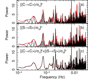
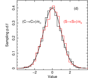
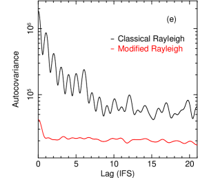
Figure 8.— Panels (a)–(c): decomposition of the $\mathcal{R}^{2}_{1}$ into its primary components, showing the cosine term in (a), the sine term in (b), and their sum in (c). Overlaid in red is the $\mathcal{R}^{2}_{1}$ periodogram. Panel (d): histogram of the standardized variables $[(C-\langle C\rangle)/\sigma_{C}]^{2}$ (black) and $[(S-\langle S\rangle)/\sigma_{S}]^{2}$ (red) plotted in panels (a) and (b) with the standard normal p.d.f. (smooth black). Panel (e): autocovariances of $R^{2}$ (black) and $\mathcal{R}^{2}_{1}$ (red) with lag in units of independent Fourier spacings.

We want to generalize the expression of Equation A4 to hold for the $k$th harmonic. Introducing the subscript $k$ on all terms to specify that they are now harmonic-specific, our matrix equation becomes

$$\mathcal{R}^{2}_{k}=\begin{pmatrix}C_{k}-\langle C_{k}\rangle\\ S_{k}-\langle S_{k}\rangle\end{pmatrix}^{\rm T}\begin{pmatrix}{\sigma^{2}}_{C_{k}}&\sigma_{C_{k}S_{k}}\\ \sigma_{C_{k}S_{k}}&{\sigma^{2}}_{S_{k}}\end{pmatrix}^{-1}\begin{pmatrix}C_{k}-\langle C_{k}\rangle\\ S_{k}-\langle S_{k}\rangle\end{pmatrix}$$ (A6)

In this case, the values of $C_{k}$ and $S_{k}$ defined in Equation A2 become

$$C_{k}=\frac{1}{N}\sum_{i=1}^{N}\cos{k\phi_{i}}\hskip 11.38109pt{\rm and}\hskip 11.38109ptS_{k}=\frac{1}{N}\sum_{i=1}^{N}\sin{k\phi_{i}},$$ (A7)

with expectation values given by

$$\langle C_{k}\rangle = \frac{1}{T}\int_{t_{1}}^{t_{2}}\cos{k\omega\/t}\,{\rm d}t=\langle\cos{k\phi}\rangle$$ (A8)

$$= \frac{1}{k\omega\/T}\left(\sin{k\omega\/t_{2}}-\sin{k\omega\/t_{1}}\right),$$

and

$$\langle S_{k}\rangle = \frac{1}{T}\int_{t_{1}}^{t_{2}}\sin{k\omega\/t}\,{\rm d}t=\langle\sin{k\phi}\rangle$$ (A9)

$$= \frac{1}{k\omega\/T}\left(\cos{k\omega\/t_{1}}-\cos{k\omega\/t_{2}}\right).$$

The variance of $C_{k}$ is

$$\sigma_{C_{k}}^{2} = \frac{1}{TN}\int_{t_{1}}^{t_{2}}\cos^{2}{k\omega\/t}\,{\rm d}t-\langle C_{k}\rangle^{2}=\frac{1}{N}Var(\cos{k\phi})$$

$$= \frac{1}{TN}\int_{t_{1}}^{t_{2}}\frac{1}{2}(1+\cos{2k\omega\/t})\,{\rm d}t-\langle C_{k}\rangle^{2}$$

$$= \frac{1}{2TN}\left(t+\frac{\sin{2k\omega\/t}}{2k\omega}\right)_{t_{1}}^{t_{2}}-\langle C_{k}\rangle^{2}$$

$$= \frac{1}{2N}\left(1+\frac{1}{k\omega\/T}(\sin{k\omega\/t_{2}}\cos{k\omega\/t_{2}}-\sin{k\omega\/t_{1}}\cos{k\omega\/t_{1}})\right)-\langle C_{k}\rangle^{2}.$$

The variance of $S_{k}$ is

$$\sigma_{S_{k}}^{2} = \frac{1}{TN}\int_{t_{1}}^{t_{2}}\sin^{2}{k\omega\/t}\,{\rm d}t-\langle S_{k}\rangle^{2}=\frac{1}{N}Var(\sin{k\phi})$$

$$= \frac{1}{TN}\int_{t_{1}}^{t_{2}}\frac{1}{2}(1-\cos{2k\omega\/t})\,{\rm d}t-\langle S_{k}\rangle^{2}$$

$$= \frac{1}{2N}\left(1-\frac{1}{k\omega\/T}(\sin{k\omega\/t_{2}}\cos{k\omega\/t_{2}}-\sin{k\omega\/t_{1}}\cos{k\omega\/t_{1}})\right)-\langle S_{k}\rangle^{2}.$$

And their covariance is given by

$$\sigma_{C_{k}S_{k}} = \langle C_{k}\cdot S_{k}\rangle-\langle C_{k}\rangle\langle S_{k}\rangle=\frac{1}{N}Cov(\cos{k\phi},\sin{k\phi})$$

$$= \frac{1}{TN}\int_{t_{1}}^{t_{2}}\cos{k\omega\/t}\sin{k\omega\/t}\,{\rm d}t-\langle C_{k}\rangle\langle S_{k}\rangle$$

$$= \frac{1}{2k\omega\/TN}\left(\sin^{2}k\omega\/t_{2}-\sin^{2}k\omega\/t_{1}\right)-\langle C_{k}\rangle\langle S_{k}\rangle.$$

Therefore, to evaluate $\mathcal{R}^{2}_{k}$ we need to compute

$$\langle C_{k}\rangle = \frac{1}{k\omega\/T}\left[\sin{k\omega\/t}\right]_{t_{1}}^{t_{2}},$$ (A13)

$$\langle S_{k}\rangle = \frac{-1}{k\omega\/T}\left[\cos{k\omega\/t}\right]_{t_{1}}^{t_{2}},$$ (A14)

$$\sigma_{C_{k}}^{2} = \frac{1}{2N}\left(1+\frac{1}{k\omega\/T}\left[\sin{k\omega\/t}\cos{k\omega\/t}\right]_{t_{1}}^{t_{2}}\right)-\langle C_{k}\rangle,$$ (A15)

$$\sigma_{S_{k}}^{2} = \frac{1}{2N}\left(1-\frac{1}{k\omega\/T}\left[\sin{k\omega\/t}\cos{k\omega\/t}\right]_{t_{1}}^{t_{2}}\right)-\langle S_{k}\rangle,$$ (A16)

$$\sigma_{C_{k}S_{k}} = \frac{1}{2k\omega\/TN}\left[\sin^{2}k\omega\/t\right]_{t_{1}}^{t_{2}}-\langle C_{k}\rangle\langle S_{k}\rangle.$$ (A17)

Figure 7 illustrates the importance of the effects discussed in relation to the Fourier power derived from the classical Rayleigh statistic (Equation A1) or the modified statistic (Equation A4, given that $k=1$). Most importantly, we see that the non-zero contribution from the analytically expected integral of sine and cosine components between independent frequencies completely dominates from mid to low frequencies, decreasing in magnitude with increasing frequency (panels (a) and (b)). In addition, note that this oscillatory behavior is also shared by the variances of $C$ and $S$ as well as by their covariance (panel (c)).

Figure 8 panels (a)–(c) show, in comparison to the periodogram drawn in red, the individual contribution and sum of the squares of the standardized variables $(C-\langle C\rangle)/\sigma_{C}$ and $(S-\langle S\rangle)/\sigma_{S}$, making it clear that the contributions of the cosine and sine terms (panels (a) and (b)) are complementary (as expected), and that their sum accounts well for the total power in the $\mathcal{R}^{2}_{1}$ periodogram (panel (c)), which implies that the covariance, $\sigma_{CS}$, in Equation A6, does not play a significant role here. In panel (d) we see that subtracting the analytical expectation ($\langle C\rangle$ and $\langle S\rangle$) from the sum of Fourier moments calculated from the phases ($C$ and $S$) results in a variable distributed around zero, and that furthermore, dividing each by the expected standard deviation ($\sigma_{C}$ and $\sigma_{S}$) yields standard normal deviates, and thus effectively independent variables.

Finally, the aim of the modifications with respect to the classical Rayleigh statistic in the $\mathcal{R}^{2}_{k}$ statistic in general and in the $\mathcal{R}^{2}_{1}$ in this case is to remove the correlation in the power estimates. Autocorrelation is always maximal for a value with itself and then drops, more or less quickly depending on the extent of the correlation between neighbors, before flattening out. In the case of the classical Rayleigh periodogram, we expect the autocovariance to oscillate with a frequency matching the IFS with an overall amplitude dropping in an exponential or power-law like fashion. In the case of the modified statistic—if the modifications successfully remove the correlation—we expect a flat curve beyond the first Fourier spacing. As shown in panel (e) of Figure 8, this is exactly what we find.

A.2. Binned Data and Point Measurements

We defined the $\mathcal{R}^{2}_{k}$ statistic for binned data and point measurements in Equation 14. It was written as

$$\mathcal{R}^{2}_{k}=\frac{\left(\sum_{i=1}^{n}\rho_{i}\cos{k\phi_{i}}\right)^{2}}{\sum_{i=1}^{n}(\rho_{i}\cos{k\phi_{i}})^{2}}+\frac{\left(\sum_{i=1}^{n}\rho_{i}\sin{k\phi_{i}}\right)^{2}}{\sum_{i=1}^{n}(\rho_{i}\sin{k\phi_{i}})^{2}}.$$ (A18)

Expressing the weights, $\rho_{i}$, explicitly as $r_{i}/\sigma_{i}^{2}$, we get

$$\mathcal{R}^{2}_{k}=\frac{\left(\sum_{i=1}^{n}r_{i}/\sigma_{i}^{2}\cos{k\phi_{i}}\right)^{2}}{\sum_{i=1}^{n}(r_{i}/\sigma_{i}^{2}\cos{k\phi_{i}})^{2}}+\frac{\left(\sum_{i=1}^{n}r_{i}/\sigma_{i}^{2}\sin{k\phi_{i}}\right)^{2}}{\sum_{i=1}^{n}(r_{i}/\sigma_{i}^{2}\sin{k\phi_{i}})^{2}}.$$ (A19)

If the uncertainty on the intensity measurements is equal—this is usually the case for infrared time series constructed from a set of individual image snapshots where the uncertainty on the measurements is calculated from the variance of the calibrator star’s intensity over the entire set of images—then $\sigma_{i}$ is constant (i.e., $\sigma$). Because it is constant, this factor that appears in all the terms can be taken out of the sums and canceled out. The statistic then becomes

$$\mathcal{R}^{2}_{k}=\frac{\left(\sum_{i=1}^{n}r_{i}\cos{k\phi_{i}}\right)^{2}}{\sum_{i=1}^{n}(r_{i}\cos{k\phi_{i}})^{2}}+\frac{\left(\sum_{i=1}^{n}r_{i}\sin{k\phi_{i}}\right)^{2}}{\sum_{i=1}^{n}(r_{i}\sin{k\phi_{i}})^{2}}.$$ (A20)

What if the uncertainties are not equal? What is the effect of the uncertainties on the periodogram? The main point of this study was given at the end of Section IV.2, namely that the size of the uncertainty on each measurement is not important in the calculation of the periodogram, but that it is the relative variations of the uncertainties, one with respect to the others, that play a role in changing the shape of the periodogram: naturally, the greater the scatter, the greater the whitening and loss of structure.

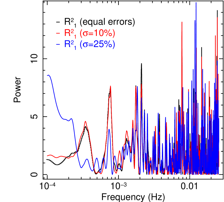
Figure 9.— Illustration of the periodogram shown in Figure 3 here calculated using the $\mathcal{R}^{2}_{k}$ statistic of Equation A19 for $k=1$, of the effects of assigning normal random uncertainties distributed with a standard deviation of 10% (red) and 25% (blue) to the intensity measurements. The reference in black is the unweighted periodogram.

Figure 9 shows the unweighted periodogram of Figure 3 in black, and two additional periodograms overlaid in red and blue. In each case random normally distributed uncertainties are assigned to the individual intensity measurements in each bin. The first shows the effect of a standard deviation of 10% in the distribution of uncertainties, and we see that the deviations from the black periodogram are small. The second shows the effects of a 25% standard deviation on the uncertainties where differences are noticeably more important.

Such a periodogram statistic in which each measurement is weighted by a potentially different uncertainty is essential in applications where we are interested in combining data from different observations, different instruments, or both, because the uncertainties from one observation to another and from one instrument to another will inevitably vary.

It is also essential when treating time series that even if from a single instrument and a single continuous observation may vary in quality from bin to bin, as is the case for the $\gamma$-ray observatory INTEGRAL, because each estimate of intensity in each bin is derived from independent snapshots whose statistical properties vary depending on factors such as the duration of the snapshot, the pointing’s direction in the sky, the position within the satellite in its orbit, the time from the passage through the radiation belts, etc. In such cases, as well as in similar ones, it would clearly be a mistake to rely on the unweighted periodogram when so many factors contribute differently to the quality of each data point in the time series.

References

- Belloni & Hasinger (1990) Belloni, T., & Hasinger, G. 1990, A&A, 227, L33
- Bozzo et al. (2012) Bozzo, E., Ferrigno, C., Türler, M., Manousakis, A., & Falanga, M. 2012, A&A, 545, A83
- Buccheri et al. (1983) Buccheri, R., Bennett, K., Bignami, G. F., et al. 1983, A&A, 128, 245
- Burderi et al. (2006) Burderi, L., Di Salvo, T., Menna, M. T., Riggio, A., & Papitto, A. 2006, ApJL, 653, L133
- de Jager (1994) de Jager, O. C. 1994, ApJ, 436, 239
- de Jager et al. (1986) de Jager, O. C., Raubenheimer, B. C., & Swanepoel, J. W. H. 1986, A&A, 170, 187
- de Jager et al. (1989) de Jager, O. C., Raubenheimer, B. C., & Swanepoel, J. W. H. 1989, A&A, 221, 180
- de Rosa et al. (2009) de Rosa, A., Ubertini, P., Campana, R., et al. 2009, MNRAS, 393, 527
- Leahy et al. (1983a) Leahy, D. A., Darbro, W., Elsner, R. F., et al. 1983a, ApJ, 266, 160
- Leahy et al. (1983b) Leahy, D. A., Elsner, R. F., & Weisskopf, M. C. 1983b, ApJ, 272, 256
- Meyer et al. (2008) Meyer, L., Do, T., Ghez, A., et al. 2008, ApJL, 688, L17
- Miyamoto et al. (1991) Miyamoto, S., Kimura, K., Kitamoto, S., Dotani, T., & Ebisawa, K. 1991, ApJ, 383, 784
- Orford (1996) Orford, K. J. 1996, Astroparticle Physics, 4, 235
- Press et al. (2002) Press, W. H., Teukolsky, S. A., Vetterling, & Flannery, B. P. 2002, Numerical Recipes in C++ : the Art of Scientific Computing (Cambridge: Cambridge Univ. Press)
- Romano et al. (2010) Romano, P., Sidoli, L., Ducci, L., et al. 2010, MNRAS, 401, 1564
- Royall (1997) Royall, R. M. 1997, Statistical Evidence, A Likelihood Paradigm (New York: Chapman & Hall/CRC)
- Scargle (1982) Scargle, J. D. 1982, ApJ, 263, 835
- Scargle (1989) Scargle, J. D. 1989, ApJ, 343, 874
- Vio et al. (2013) Vio, R., Diaz-Trigo, M., & Andreani, P. 2013, A&C, 1, 5