Cascade R-CNN: Delving into High Quality Object Detection

Abstract

In object detection, an intersection over union (IoU) threshold is required to define positives and negatives. An object detector, trained with low IoU threshold, e.g. 0.5, usually produces noisy detections. However, detection performance tends to degrade with increasing the IoU thresholds. Two main factors are responsible for this: 1) overfitting during training, due to exponentially vanishing positive samples, and 2) inference-time mismatch between the IoUs for which the detector is optimal and those of the input hypotheses. A multi-stage object detection architecture, the Cascade R-CNN, is proposed to address these problems. It consists of a sequence of detectors trained with increasing IoU thresholds, to be sequentially more selective against close false positives. The detectors are trained stage by stage, leveraging the observation that the output of a detector is a good distribution for training the next higher quality detector. The resampling of progressively improved hypotheses guarantees that all detectors have a positive set of examples of equivalent size, reducing the overfitting problem. The same cascade procedure is applied at inference, enabling a closer match between the hypotheses and the detector quality of each stage. A simple implementation of the Cascade R-CNN is shown to surpass all single-model object detectors on the challenging COCO dataset. Experiments also show that the Cascade R-CNN is widely applicable across detector architectures, achieving consistent gains independently of the baseline detector strength. The code will be made available at https://github.com/zhaoweicai/cascade-rcnn.

1 Introduction

Object detection is a complex problem, requiring the solution of two main tasks. First, the detector must solve the recognition problem, to distinguish foreground objects from background and assign them the proper object class labels. Second, the detector must solve the localization problem, to assign accurate bounding boxes to different objects. Both of these are particularly difficult because the detector faces many “close” false positives, corresponding to “close but not correct” bounding boxes. The detector must find the true positives while suppressing these close false positives.

Many of the recently proposed object detectors are based on the two-stage R-CNN framework [12, 11, 27, 21], where detection is framed as a multi-task learning problem that combines classification and bounding box regression. Unlike object recognition, an intersection over union (IoU) threshold is required to define positives/negatives. However, the commonly used threshold values $u$, typically $u=0.5$, establish quite a loose requirement for positives. The resulting detectors frequently produce noisy bounding boxes, as shown in Figure 1 (a). Hypotheses that most humans would consider close false positives frequently pass the $IoU\geq 0.5$ test. While the examples assembled under the $u=0.5$ criterion are rich and diversified, they make it difficult to train detectors that can effectively reject close false positives.

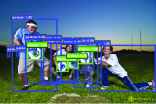
(a) Detection of $u=0.5$

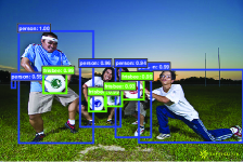
(b) Detection of $u=0.7$

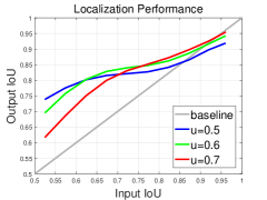
(c) Regressor

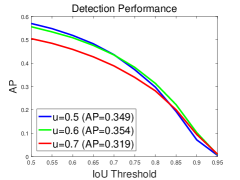
(d) Detector

Figure 1: The detection outputs, localization and detection performance of object detectors of increasing IoU threshold $u$.

In this work, we define the quality of an hypothesis as its IoU with the ground truth, and the quality of the detector as the IoU threshold $u$ used to train it. The goal is to investigate the, so far, poorly researched problem of learning high quality object detectors, whose outputs contain few close false positives, as shown in Figure 1 (b). The basic idea is that a single detector  can only be optimal for a single quality level. This is known in the cost-sensitive learning literature [7, 24], where the optimization of different points of the receiver operating characteristic (ROC) requires different loss functions. The main difference is that we consider the optimization for a given IoU threshold, rather than false positive rate.

The idea is illustrated by Figure 1 (c) and (d), which present the localization and detection performance, respectively, of three detectors trained with IoU thresholds of $u=0.5,0.6,0.7$. The localization performance is evaluated as a function of the IoU of the input proposals, and the detection performance as a function of IoU threshold, as in COCO [20]. Note that, in Figure 1 (c), each bounding box regressor performs best for examples of IoU close to the threshold that the detector was trained. This also holds for detection performance, up to overfitting. Figure 1 (d) shows that, the detector of $u=0.5$ outperforms the detector of $u=0.6$ for low IoU examples, underperforming it at higher IoU levels. In general, a detector optimized at a single IoU level is not necessarily optimal at other levels. These observations suggest that higher quality detection requires a closer quality match between the detector and the hypotheses that it processes. In general, a detector can only have high quality if presented with high quality proposals.

However, to produce a high quality detector, it does not suffice to simply increase $u$ during training. In fact, as seen for the detector of $u=0.7$ of Figure 1 (d), this can degrade detection performance. The problem is that the distribution of hypotheses out of a proposal detector is usually heavily imbalanced towards low quality. In general, forcing larger IoU thresholds leads to an exponentially smaller numbers of positive training samples. This is particularly problematic for neural networks, which are known to be very example intensive, and makes the “high $u$” training strategy quite prone to overfitting. Another difficulty is the mismatch between the quality of the detector and that of the testing hypotheses at inference. As shown in Figure 1, high quality detectors are only necessarily optimal for high quality hypotheses. The detection could be suboptimal when they are asked to work on the hypotheses of other quality levels.

In this paper, we propose a new detector architecture, Cascade R-CNN, that addresses these problems. It is a multi-stage extension of the R-CNN, where detector stages deeper into the cascade are sequentially more selective against close false positives. The cascade of R-CNN stages are trained sequentially, using the output of one stage to train the next. This is motivated by the observation that the output IoU of a regressor is almost invariably better than the input IoU. This observation can be made in Figure 1 (c), where all plots are above the gray line. It suggests that the output of a detector trained with a certain IoU threshold is a good distribution to train the detector of the next higher IoU threshold. This is similar to boostrapping methods commonly used to assemble datasets in object detection literature [31, 8]. The main difference is that the resampling procedure of the Cascade R-CNN does not aim to mine hard negatives. Instead, by adjusting bounding boxes, each stage aims to find a good set of close false positives for training the next stage. When operating in this manner, a sequence of detectors adapted to increasingly higher IoUs can beat the overfitting problem, and thus be effectively trained. At inference, the same cascade procedure is applied. The progressively improved hypotheses are better matched to the increasing detector quality at each stage. This enables higher detection accuracies, as suggested by Figure 1 (c) and (d).

The Cascade R-CNN is quite simple to implement and trained end-to-end. Our results show that a vanilla implementation, without any bells and whistles, surpasses all previous state-of-the-art single-model detectors by a large margin, on the challenging COCO detection task [20], especially under the higher quality evaluation metrics. In addition, the Cascade R-CNN can be built with any two-stage object detector based on the R-CNN framework. We have observed consistent gains (of 2$\sim$4 points), at a marginal increase in computation. This gain is independent of the strength of the baseline object detectors. We thus believe that this simple and effective detection architecture can be of interest for many object detection research efforts.

2 Related Work

Due to the success of the R-CNN [12] architecture, the two-stage formulation of the detection problems, by combining a proposal detector and a region-wise classifier has become predominant in the recent past. To reduce redundant CNN computations in the R-CNN, the SPP-Net [15] and Fast-RCNN [11] introduced the idea of region-wise feature extraction, significantly speeding up the overall detector. Later, the Faster-RCNN [27] achieved further speeds-up by introducing a Region Proposal Network (RPN). This architecture has become a leading object detection framework. Some more recent works have extended it to address various problems of detail. For example, the R-FCN [4] proposed efficient region-wise fully convolutions without accuracy loss, to avoid the heavy region-wise CNN computations of the Faster-RCNN; while the MS-CNN [1] and FPN [21] detect proposals at multiple output layers, so as to alleviate the scale mismatch between the RPN receptive fields and actual object size, for high-recall proposal detection.

Alternatively, one-stage object detection architectures have also become popular, mostly due to their computational efficiency. These architectures are close to the classic sliding window strategy [31, 8]. YOLO [26] outputs very sparse detection results by forwarding the input image once. When implemented with an efficient backbone network, it enables real time object detection with fair performance. SSD [23] detects objects in a way similar to the RPN [27], but uses multiple feature maps at different resolutions to cover objects at various scales. The main limitation of these architectures is that their accuracies are typically below that of two-stage detectors. Recently, RetinaNet [22] was proposed to address the extreme foreground-background class imbalance in dense object detection, achieving better results than state-of-the-art two-stage object detectors.

Some explorations in multi-stage object detection have also been proposed. The multi-region detector [9] introduced iterative bounding box regression, where a R-CNN is applied several times, to produce better bounding boxes. CRAFT [33] and AttractioNet [10] used a multi-stage procedure to generate accurate proposals, and forwarded them to a Fast-RCNN. [19, 25] embedded the classic cascade architecture of [31] in object detection networks. [3] iterated a detection and a segmentation task alternatively, for instance segmentation.

3 Object Detection

In this paper, we extend the two-stage architecture of the Faster-RCNN [27, 21], shown in Figure 3 (a). The first stage is a proposal sub-network (“H0”), applied to the entire image, to produce preliminary detection hypotheses, known as object proposals. In the second stage, these hypotheses are then processed by a region-of-interest detection sub-network (“H1”), denoted as detection head. A final classification score (“C”) and a bounding box (“B”) are assigned to each hypothesis. We focus on modeling a multi-stage detection sub-network, and adopt, but are not limited to, the RPN [27] for proposal detection.

3.1 Bounding Box Regression

A bounding box $\textbf{b}=(b_{x},b_{y},b_{w},b_{h})$ contains the four coordinates of an image patch $x$. The task of bounding box regression is to regress a candidate bounding box b into a target bounding box g, using a regressor $f(x,\textbf{b})$. This is learned from a training sample $\{\textbf{g}_{i},\textbf{b}_{i}\}$, so as to minimize the bounding box risk

$${\cal R}_{loc}[f]=\sum_{i=1}^{N}L_{loc}(f(x_{i},\textbf{b}_{i}),\textbf{g}_{i}),$$ (1)

where $L_{loc}$ was a $L_{2}$ loss function in R-CNN [12], but updated to a smoothed $L_{1}$ loss function in Fast-RCNN [11]. To encourage a regression invariant to scale and location, $L_{loc}$ operates on the distance vector $\Delta=(\delta_{x},\delta_{y},\delta_{w},\delta_{h})$ defined by

$$\begin{array}[]{cl}\delta_{x}=(g_{x}-b_{x})/b_{w},\quad\delta_{y}=(g_{y}-b_{y})/b_{h}\\ \delta_{w}=\log(g_{w}/b_{w}),\quad\delta_{h}=\log(g_{h}/b_{h}).\end{array}$$ (2)

Since bounding box regression usually performs minor adjustments on $b$, the numerical values of (2) can be very small. Hence, the risk of (1) is usually much smaller than the classification risk. To improve the effectiveness of multi-task learning, $\Delta$ is usually normalized by its mean and variance, i.e. $\delta_{x}$ is replaced by $\delta_{x}^{\prime}=(\delta_{x}-\mu_{x})/\sigma_{x}$. This is widely used in the literature [27, 1, 4, 21, 14].

Some works [9, 10, 16] have argued that a single regression step of $f$ is insufficient for accurate localization. Instead, $f$ is applied iteratively, as a post-processing step

$$f^{\prime}(x,\textbf{b})=f\circ{f}\circ\cdots\circ{f}(x,\textbf{b}),$$ (3)

to refine a bounding box b. This is called iterative bounding box regression, denoted as iterative BBox. It can be implemented with the inference architecture of Figure 3 (b) where all heads are the same. This idea, however, ignores two problems. First, as shown in Figure 1, a regressor $f$ trained at $u=0.5$, is suboptimal for hypotheses of higher IoUs. It actually degrades bounding boxes of IoU larger than $0.85$. Second, as shown in Figure 2, the distribution of bounding boxes changes significantly after each iteration. While the regressor is optimal for the initial distribution it can be quite suboptimal after that. Due to these problems, iterative BBox requires a fair amount of human engineering, in the form of proposal accumulation, box voting, etc. [9, 10, 16], and has somewhat unreliable gains. Usually, there is no benefit beyond applying $f$ twice.

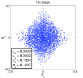
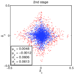
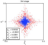
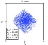
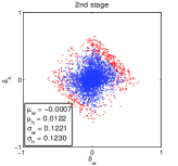
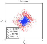
Figure 2: Sequential $\Delta$ distribution (without normalization) at different cascade stage. Red dots are outliers when using increasing IoU thresholds, and the statistics are obtained after outlier removal.

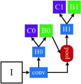
(a) Faster R-CNN

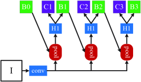
(b) Iterative BBox at inference

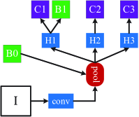
(c) Integral Loss

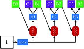
(d) Cascade R-CNN

Figure 3: The architectures of different frameworks. “I” is input image, “conv” backbone convolutions, “pool” region-wise feature extraction, “H” network head, “B” bounding box, and “C” classification. “B0” is proposals in all architectures.

3.2 Classification

The classifier is a function $h(x)$ that assigns an image patch $x$ to one of $M+1$ classes, where class $0$ contains background and the remaining the objects to detect. $h(x)$ is a $M+1$-dimensional estimate of the posterior distribution over classes, i.e. $h_{k}(x)=p(y=k|x)$, where $y$ is the class label. Given a training set $(x_{i},y_{i})$, it is learned by minimizing a classification risk

$${\cal R}_{cls}[h]=\sum_{i=1}^{N}L_{cls}(h(x_{i}),y_{i}),$$ (4)

where $L_{cls}$ is the classic cross-entropy loss.

3.3 Detection Quality

Since a bounding box usually includes an object and some amount of background, it is difficult to determine if a detection is positive or negative. This is usually addressed by the IoU metric. If the IoU is above a threshold $u$, the patch is considered an example of the class. Thus, the class label of a hypothesis $x$ is a function of $u$,

$$y=\left\{\begin{array}[]{cl}g_{y},&\quad\textrm{$IoU(x,g)\geq{u}$}\\ 0,&\quad\textrm{otherwise}\end{array}\right.$$ (5)

where $g_{y}$ is the class label of the ground truth object $g$. This IoU threshold $u$ defines the quality of a detector.

Object detection is challenging because, no matter threshold, the detection setting is highly adversarial. When $u$ is high, the positives contain less background, but it is difficult to assemble enough positive training examples. When $u$ is low, a richer and more diversified positive training set is available, but the trained detector has little incentive to reject close false positives. In general, it is very difficult to ask a single classifier to perform uniformly well over all IoU levels. At inference, since the majority of the hypotheses produced by a proposal detector, e.g. RPN [27] or selective search [30], have low quality, the detector must be more discriminant for lower quality hypotheses. A standard compromise between these conflicting requirements is to settle on $u=0.5$. This, however, is a relatively low threshold, leading to low quality detections that most humans consider close false positives, as shown in Figure 1 (a).

A naïve solution is to develop an ensemble of classifiers, with the architecture of Figure 3 (c), optimized with a loss that targets various quality levels,

$$L_{cls}(h(x),y)=\sum_{u\in{U}}L_{cls}(h_{u}(x),y_{u}),$$ (6)

where $U$ is a set of IoU thresholds. This is closely related to the integral loss of [34], in which $U=\{0.5,0.55,\cdots,0.75\}$, designed to fit the evaluation metric of the COCO challenge. By definition, the classifiers need to be ensembled at inference. This solution fails to address the problem that the different losses of (6) operate on different numbers of positives. As shown in the first figure of Figure 4, the set of positive samples decreases quickly with $u$. This is particularly problematic because the high quality classifiers are prone to overfitting. In addition, those high quality classifiers are required to process proposals of overwhelming low quality at inference, for which they are not optimized. Due to all this, the ensemble of (6) fails to achieve higher accuracy at most quality levels, and the architecture has very little gain over that of Figure 3 (a).

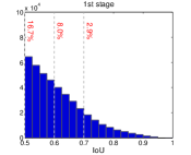
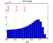
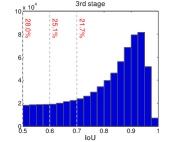
Figure 4: The IoU histogram of training samples. The distribution at 1st stage is the output of RPN. The red numbers are the positive percentage higher than the corresponding IoU threshold.

4 Cascade R-CNN

In this section we introduce the proposed Cascade R-CNN object detection architecture of Figure 3 (d).

4.1 Cascaded Bounding Box Regression

As seen in Figure 1 (c), it is very difficult to ask a single regressor to perform perfectly uniformly at all quality levels. The difficult regression task can be decomposed into a sequence of simpler steps, inspired by the works of cascade pose regression [6] and face alignment [2, 32]. In the Cascade R-CNN, it is framed as a cascaded regression problem, with the architecture of Figure 3 (d). This relies on a cascade of specialized regressors

$$f(x,\textbf{b})=f_{T}\circ{f}_{T-1}\circ\cdots\circ{f}_{1}(x,\textbf{b}),$$ (7)

where $T$ is the total number of cascade stages. Note that each regressor $f_{t}$ in the cascade is optimized w.r.t. the sample distribution $\{\textbf{b}^{t}\}$ arriving at the corresponding stage, instead of the initial distribution of $\{\textbf{b}^{1}\}$. This cascade improves hypotheses progressively.

It differs from the iterative BBox architecture of Figure 3 (b) in several ways. First, while iterative BBox is a post-processing procedure used to improve bounding boxes, cascaded regression is a resampling procedure that changes the distribution of hypotheses to be processed by the different stages. Second, because it is used at both training and inference, there is no discrepancy between training and inference distributions. Third, the multiple specialized regressors $\{f_{T},f_{T-1},\cdots,f_{1}\}$ are optimized for the resampled distributions of the different stages. This opposes to the single $f$ of (3), which is only optimal for the initial distribution. These differences enable more precise localization than iterative BBox, with no further human engineering.

As discussed in Section 3.1, $\Delta=(\delta_{x},\delta_{y},\delta_{w},\delta_{h})$ in (2) needs to be normalized by its mean and variance for effective multi-task learning. After each regression stage, these statistics will evolve sequentially, as displayed in Figure 2. At training, the corresponding statistics are used to normalize $\Delta$ at each stage.

4.2 Cascaded Detection

As shown in the left of Figure 4, the distribution of the initial hypotheses, e.g. RPN proposals, is heavily tilted towards low quality. This inevitably induces ineffective learning of higher quality classifiers. The Cascade R-CNN addresses the problem by relying on cascade regression as a resampling mechanism. This is is motivated by the fact that in Figure 1 (c) all curves are above the diagonal gray line, i.e. a bounding box regressor trained for a certain $u$ tends to produce bounding boxes of higher IoU. Hence, starting from a set of examples $(x_{i},\textbf{b}_{i})$, cascade regression successively resamples an example distribution $(x^{\prime}_{i},\textbf{b}^{\prime}_{i})$ of higher IoU. In this manner, it is possible to keep the set of positive examples of the successive stages at a roughly constant size, even when the detector quality (IoU threshold) is increased. This is illustrated in Figure 4, where the distribution tilts more heavily towards high quality examples after each resampling step. Two consequences ensue. First, there is no overfitting, since examples are plentiful at all levels. Second, the detectors of the deeper stages are optimized for higher IoU thresholds. Note that, some outliers are sequentially removed by increasing IoU thresholds, as illustrated in Figure 2, enabling a better trained sequence of specialized detectors.

At each stage $t$, the R-CNN includes a classifier $h_{t}$ and a regressor $f_{t}$ optimized for IoU threshold $u^{t}$, where $u^{t}>u^{t-1}$. This is guaranteed by minimizing the loss

$$L(x^{t},g)=L_{cls}(h_{t}(x^{t}),y^{t})+\lambda[y^{t}\geq{1}]L_{loc}(f_{t}(x^{t},\textbf{b}^{t}),\textbf{g}),$$ (8)

where $\textbf{b}^{t}=f_{t-1}(x^{t-1},\textbf{b}^{t-1})$, $g$ is the ground truth object for $x^{t}$, $\lambda=1$ the trade-off coefficient, $[\cdot]$ the indicator function, and $y^{t}$ is the label of $x^{t}$ given $u^{t}$ by (5). Unlike the integral loss of (6), this guarantees a sequence of effectively trained detectors of increasing quality. At inference, the quality of the hypotheses is sequentially improved, by applications of the same cascade procedure, and higher quality detectors are only required to operate on higher quality hypotheses. This enables high quality object detection, as suggested by Figure 1 (c) and (d).

5 Experimental Results

The Cascade R-CNN was evaluated on MS-COCO 2017 [20], which contains $\sim$118k images for training, 5k for validation (val) and $\sim$20k for testing without provided annotations (test-dev). The COCO-style Average Precision (AP) averages AP across IoU thresholds from 0.5 to 0.95 with an interval of 0.05. These evaluation metrics measure the detection performance of various qualities. All models were trained on COCO training set, and evaluated on val set. Final results were also reported on test-dev set.

5.1 Implementation Details

All regressors are class agnostic for simplicity. All cascade detection stages in Cascade R-CNN have the same architecture, which is the head of the baseline detection network. In total, Cascade R-CNN have four stages, one RPN and three for detection with $U=\{0.5,0.6,0.7\}$, unless otherwise noted. The sampling of the first detection stage follows [11, 27]. In the following stages, resampling is implemented by simply using the regressed outputs from the previous stage, as in Section 4.2. No data augmentation was used except standard horizontal image flipping. Inference was performed on a single image scale, with no further bells and whistles. All baseline detectors were reimplemented with Caffe [18], on the same codebase for fair comparison.

5.1.1 Baseline Networks

To test the versatility of the Cascade R-CNN, experiments were performed with three popular baseline detectors: Faster-RCNN with backbone VGG-Net [29], R-FCN [4] and FPN [21] with ResNet backbone [16]. These baselines have a wide range of detection performances. Unless noted, their default settings were used. End-to-end training was used instead of multi-step training.

Faster-RCNN:

The network head has two fully connected layers. To reduce parameters, we used [13] to prune less important connections. 2048 units were retained per fully connected layer and dropout layers were removed. Training started with a learning rate of 0.002, reduced by a factor of 10 at 60k and 90k iterations, and stopped at 100k iterations, on 2 synchronized GPUs, each holding 4 images per iteration. 128 RoIs were used per image.

R-FCN:

R-FCN adds a convolutional, a bounding box regression, and a classification layer to the ResNet. All heads of the Cascade R-CNN have this structure. Online hard negative mining [28] was not used. Training started with a learning rate of 0.003, which was decreased by a factor of 10 at 160k and 240k iterations, and stopped at 280k iterations, on 4 synchronized GPUs, each holding one image per iteration. 256 RoIs were used per image.

FPN:

Since no source code is publicly available yet for FPN, our implementation details could be different. RoIAlign [14] was used for a stronger baseline. This is denoted as FPN+ and was used in all ablation studies. As usual, ResNet-50 was used for ablation studies, and ResNet-101 for final detection. Training used a learning rate of 0.005 for 120k iterations and 0.0005 for the next 60k iterations, on 8 synchronized GPUs, each holding one image per iteration. 256 RoIs were used per image.

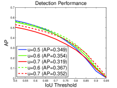
(a)

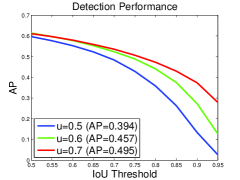
(b)

Figure 5: (a) is detection performance of individually trained detectors, with their own proposals (solid curves) or Cascade R-CNN stage proposals (dashed curves), and (b) is by adding ground truth to the proposal set.

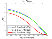
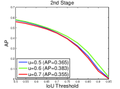
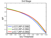
Figure 6: The detection performance of all Cascade R-CNN detectors at all cascade stages.

5.2 Quality Mismatch

Figure 5 (a) shows the AP curves of three individually trained detectors of increasing IoU thresholds of $U=\{0.5,0.6,0.7\}$. The detector of $u=0.5$ outperforms the detector of $u=0.6$ at low IoU levels, but underperforms it at higher levels. However, the detector of $u=0.7$ underperforms the other two. To understand why this happens, we changed the quality of the proposals at inference. Figure 5 (b) shows the results obtained when ground truth bounding boxes were added to the set of proposals. While all detectors improve, the detector of $u=0.7$ has the largest gains, achieving the best performance at almost all IoU levels. These results suggest two conclusions. First, $u=0.5$ is not a good choice for precise detection, simply more robust to low quality proposals. Second, highly precise detection requires hypotheses that match the detector quality. Next, the original detector proposals were replaced by the Cascade R-CNN proposals of higher quality ($u=0.6$ and $u=0.7$ used the 2nd and 3rd stage proposals, respectively). Figure 5 (a) also suggests that the performance of the two detectors is significantly improved when the testing proposals closer match the detector quality.

Testing all Cascade R-CNN detectors at all cascade stages produced similar observations. Figure 6 shows that each detector was improved when used more precise hypotheses, while higher quality detector had larger gain. For example, the detector of $u=0.7$ performed poorly for the low quality proposals of the 1st stage, but much better for the more precise hypotheses available at the deeper cascade stages. In addition, the jointly trained detectors of Figure 6 outperformed the individually trained detectors of Figure 5 (a), even when the same proposals were used. This indicates that the detectors are better trained within the Cascade R-CNN framework.

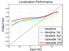
(a)

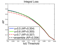
(b)

Figure 7: (a) is the localization comparison, and (b) is the detection performance of individual classifiers in the integral loss detector.

5.3 Comparison with Iterative BBox and Integral Loss

In this section, we compare the Cascade R-CNN to iterative BBox and the integral loss detector. Iterative BBox was implemented by applying the FPN+ baseline iteratively, three times. The integral loss detector has the same number of classification heads as the Cascade R-CNN, with $U=\{0.5,0.6,0.7\}$.

Localization:

The localization performances of cascade regression and iterative BBox are compared in Figure 7 (a). The use of a single regressor degrades localization for hypotheses of high IoU. This effect accumulates when the regressor is applied iteratively, as in iterative BBox, and performance actually drops. Note the very poor performance of iterative BBox after 3 iterations. On the contrary, the cascade regressor has better performance at later stages, outperforming iterative BBox at almost all IoU levels.

	AP	AP50	AP60	AP70	AP80	AP90
FPN+ baseline	34.9	57.0	51.9	43.6	29.7	7.1
Iterative BBox	35.4	57.2	52.1	44.2	30.4	8.1
Integral Loss	35.4	57.3	52.5	44.4	29.9	6.9
Cascade R-CNN	38.9	57.8	53.4	46.9	35.8	15.8

Table 1: The comparison with iterative BBox and integral loss.

Integral Loss:

The detection performances of all classifiers in the integral loss detector, sharing a single regressor, are shown in Figure 7 (b). The classifier of $u=0.6$ is the best at all IoU levels, while the classifier of $u=0.7$ is the worst. The ensemble of all classifiers shows no visible gain.

Table 1 shows, both iterative BBox and integral loss detector improve the baseline detector marginally. The cascade R-CNN has the best performance for all evaluation metrics. The gains are mild for low IoU thresholds but significant for the higher ones.

test stage	AP	AP50	AP60	AP70	AP80	AP90
1	35.5	57.2	52.4	44.1	30.5	8.1
2	38.3	57.9	53.4	46.4	35.2	14.2
3	38.3	56.6	52.2	46.3	35.7	15.9
$\overline{1\sim{2}}$	38.5	58.2	53.8	46.7	35.0	14.0
$\overline{1\sim{3}}$	38.9	57.8	53.4	46.9	35.8	15.8
FPN+ baseline	34.9	57.0	51.9	43.6	29.7	7.1

Table 2: The stage performance of Cascade R-CNN. $\overline{1\sim{3}}$ indicates the ensemble of three classifiers on the 3rd stage proposals.

5.4 Ablation Experiments

Ablation experiments were also performed.

Stage-wise Comparison:

Table 2 summarizes stage performance. The 1st stage already outperforms the baseline detector, due to the benefits of multi-stage multi-task learning. The 2nd stage improves performance substantially, and the 3rd is equivalent to the 2nd. This differs from the integral loss detector, where the higher IOU classifier is relatively weak. While the former (later) stage is better at low (high) IoU metrics, the ensemble of all classifiers is the best overall.

IoU Thresholds:

A preliminary Cascade R-CNN was trained using the same IoU threshold $u=0.5$ for all heads. In this case, the stages differ only in the hypotheses they receive. Each stage is trained with the corresponding hypotheses, i.e. accounting for the distributions of Figure 2. The first row of Table 3 shows that the cascade improves on the baseline detector. This suggests the importance of optimizing stages for the corresponding sample distributions. The second row shows that, by increasing the stage threshold $u$, the detector can be made more selective against close false positives and specialized for more precise hypotheses, leading to additional gains. This supports the conclusions of Section 4.2.

Regression Statistics:

Exploiting the progressively updated regression statistics, of Figure 2, helps the effective multi-task learning of classification and regression. Its benefit is noted by comparing the models with/without it in Table 3. The learning is not sensitive to these statistics.

IoU$\uparrow$	stat	AP	AP50	AP60	AP70	AP80	AP90
		36.8	57.8	52.9	45.4	32.0	10.7
✓		38.5	58.4	54.1	47.1	35.0	13.1
	✓	37.5	57.8	53.1	45.5	33.3	13.1
✓	✓	38.9	57.8	53.4	46.9	35.8	15.8

Table 3: The ablation experiments. “IoU$\uparrow$” means increasing IoU thresholds, and “stat” exploiting sequential regression statistics.

# stages	test stage	AP	AP50	AP60	AP70	AP80	AP90
1	1	34.9	57.0	51.9	43.6	29.7	7.1
2	$\overline{1\sim{2}}$	38.2	58.0	53.6	46.7	34.6	13.6
3	$\overline{1\sim{3}}$	38.9	57.8	53.4	46.9	35.8	15.8
4	$\overline{1\sim{3}}$	38.9	57.4	53.2	46.8	36.0	16.0
4	$\overline{1\sim{4}}$	38.6	57.2	52.8	46.2	35.5	16.3

Table 4: The impact of the number of stages in Cascade R-CNN.

Number of Stages:

The impact of the number of stages is summarized in Table 4. Adding a second detection stage significantly improves the baseline detector. Three detection stages still produce non-trivial improvement, but the addition of a 4th stage ($u=0.75$) led to a slight performance decrease. Note, however, that while the overall AP performance degrades, the four-stage cascade has the best performance for high IoU levels. The three-stage cascade achieves the best trade-off.

	backbone	AP	AP50	AP75	APS	APM	APL
YOLOv2 [26]	DarkNet-19	21.6	44.0	19.2	5.0	22.4	35.5
SSD513 [23]	ResNet-101	31.2	50.4	33.3	10.2	34.5	49.8
RetinaNet [22]	ResNet-101	39.1	59.1	42.3	21.8	42.7	50.2
Faster R-CNN+++ [16]*	ResNet-101	34.9	55.7	37.4	15.6	38.7	50.9
Faster R-CNN w FPN [21]	ResNet-101	36.2	59.1	39.0	18.2	39.0	48.2
Faster R-CNN w FPN+ (ours)	ResNet-101	38.8	61.1	41.9	21.3	41.8	49.8
Faster R-CNN by G-RMI [17]	Inception-ResNet-v2	34.7	55.5	36.7	13.5	38.1	52.0
Deformable R-FCN [5]*	Aligned-Inception-ResNet	37.5	58.0	40.8	19.4	40.1	52.5
Mask R-CNN [14]	ResNet-101	38.2	60.3	41.7	20.1	41.1	50.2
AttractioNet [10]*	VGG16+Wide ResNet	35.7	53.4	39.3	15.6	38.0	52.7
Cascade R-CNN	ResNet-101	42.8	62.1	46.3	23.7	45.5	55.2

Table 5: Comparison with the state-of-the-art single-model detectors on COCO test-dev. The entries denoted by “*” used bells and whistles at inference.

	backbone	cascade	train	test	param	val (5k)						test-dev (20k)
			speed	speed		AP	AP50	AP75	APS	APM	APL	AP	AP50	AP75	APS	APM	APL
Faster R-CNN	VGG	✗	0.12s	0.075s	278M	23.6	43.9	23.0	8.0	26.2	35.5	23.5	43.9	22.6	8.1	25.1	34.7
		✓	0.14s	0.115s	704M	27.0	44.2	27.7	8.6	29.1	42.2	26.9	44.3	27.8	8.3	28.2	41.1
R-FCN	ResNet-50	✗	0.19s	0.07s	133M	27.0	48.7	26.9	9.8	30.9	40.3	27.1	49.0	26.9	10.4	29.7	39.2
		✓	0.24s	0.075s	184M	31.1	49.8	32.8	10.4	34.4	48.5	30.9	49.9	32.6	10.5	33.1	46.9
R-FCN	ResNet-101	✗	0.23s	0.075s	206M	30.3	52.2	30.8	12.0	34.7	44.3	30.5	52.9	31.2	12.0	33.9	43.8
		✓	0.29s	0.083s	256M	33.3	52.0	35.2	11.8	37.2	51.1	33.3	52.6	35.2	12.1	36.2	49.3
FPN+	ResNet-50	✗	0.30s	0.095s	165M	36.5	58.6	39.2	20.8	40.0	47.8	36.5	59.0	39.2	20.3	38.8	46.4
		✓	0.33s	0.115s	272M	40.3	59.4	43.7	22.9	43.7	54.1	40.6	59.9	44.0	22.6	42.7	52.1
FPN+	ResNet-101	✗	0.38s	0.115s	238M	38.5	60.6	41.7	22.1	41.9	51.1	38.8	61.1	41.9	21.3	41.8	49.8
		✓	0.41s	0.14s	345M	42.7	61.6	46.6	23.8	46.2	57.4	42.8	62.1	46.3	23.7	45.5	55.2

Table 6: Detailed comparison on multiple popular baseline object detectors. All speeds are reported per image on a single Titan Xp GPU.

5.5 Comparison with the state-of-the-art

The Cascade R-CNN, based on FPN+ and ResNet-101 backbone, is compared to state-of-the-art single-model object detectors in Table 5. The settings are as described in Section 5.1.1, but a total of 280k training iterations were run and the learning rate dropped at 160k and 240k iterations. The number of RoIs was also increased to 512. The first group of detectors on Table 5 are one-stage detectors, the second group two-stage, and the last group multi-stage (3-stages+RPN for the Cascade R-CNN). All the compared state-of-the-art detectors were trained with $u=0.5$. It is noted that our FPN+ implementation is better than the original FPN [21], providing a very strong baseline. In addition, the extension from FPN+ to Cascade R-CNN improved performance by $\sim$4 points. The Cascade R-CNN also outperformed all single-model detectors by a large margin, under all evaluation metrics. This includes the single-model entries of the COCO challenge winners in 2015 and 2016 (Faster R-CNN+++ [16], and G-RMI [17]), and the very recent Deformable R-FCN [5], RetinaNet [22] and Mask R-CNN [14]. The best multi-stage detector on COCO, AttractioNet [10], used iterative BBox for proposal generation. Although many enhancements were used in AttractioNet, the vanilla Cascade R-CNN still outperforms it by 7.1 points. Note that, unlike Mask R-CNN, no segmentation information is exploited in the Cascade R-CNN. Finally, the vanilla single-model Cascade R-CNN also surpasses the heavily engineered ensemble detectors that won the COCO challenge in 2015 and 2016 (AP 37.4 and 41.6, respectively).

5.6 Generalization Capacity

Three-stage Cascade R-CNN of all three baseline detectors are compared in Table 6. All settings are as above, with the changes of Section 5.5 for FPN+.

Detection Performance:

Again, our implementations are better than the original detectors [27, 4, 21]. Still, the Cascade R-CNN improves on these baselines consistently by 2$\sim$4 points, independently of their strength. These gains are also consistent on val and test-dev. These results suggest that the Cascade R-CNN is widely applicable across detector architectures.

Parameter and Timing:

The number of the Cascade R-CNN parameters increases with the number of cascade stages. The increase is linear in the parameter number of the baseline detector heads. In addition, because the computational cost of a detection head is usually small when compared to the RPN, the computational overhead of the Cascade R-CNN is small, at both training and testing.

6 Conclusion

In this paper, we proposed a multi-stage object detection framework, the Cascade R-CNN, for the design of high quality object detectors. This architecture was shown to avoid the problems of overfitting at training and quality mismatch at inference. The solid and consistent detection improvements of the Cascade R-CNN on the challenging COCO dataset suggest the modeling and understanding of various concurring factors are required to advance object detection. The Cascade R-CNN was shown to be applicable to many object detection architectures. We believe that it can be useful to many future object detection research efforts.

Acknowledgment

We would like to thank Kaiming He for valuable discussions.

References

- [1] Z. Cai, Q. Fan, R. S. Feris, and N. Vasconcelos. A unified multi-scale deep convolutional neural network for fast object detection. In ECCV, pages 354–370, 2016.
- [2] X. Cao, Y. Wei, F. Wen, and J. Sun. Face alignment by explicit shape regression. In CVPR, pages 2887–2894, 2012.
- [3] J. Dai, K. He, and J. Sun. Instance-aware semantic segmentation via multi-task network cascades. In CVPR, pages 3150–3158, 2016.
- [4] J. Dai, Y. Li, K. He, and J. Sun. R-FCN: object detection via region-based fully convolutional networks. In NIPS, pages 379–387, 2016.
- [5] J. Dai, H. Qi, Y. Xiong, Y. Li, G. Zhang, H. Hu, and Y. Wei. Deformable convolutional networks. In ICCV, 2017.
- [6] P. Dollár, P. Welinder, and P. Perona. Cascaded pose regression. In CVPR, pages 1078–1085, 2010.
- [7] C. Elkan. The foundations of cost-sensitive learning. In IJCAI, pages 973–978, 2001.
- [8] P. F. Felzenszwalb, R. B. Girshick, D. A. McAllester, and D. Ramanan. Object detection with discriminatively trained part-based models. IEEE Trans. Pattern Anal. Mach. Intell., 32(9):1627–1645, 2010.
- [9] S. Gidaris and N. Komodakis. Object detection via a multi-region and semantic segmentation-aware CNN model. In ICCV, pages 1134–1142, 2015.
- [10] S. Gidaris and N. Komodakis. Attend refine repeat: Active box proposal generation via in-out localization. In BMVC, 2016.
- [11] R. B. Girshick. Fast R-CNN. In ICCV, pages 1440–1448, 2015.
- [12] R. B. Girshick, J. Donahue, T. Darrell, and J. Malik. Rich feature hierarchies for accurate object detection and semantic segmentation. In CVPR, pages 580–587, 2014.
- [13] S. Han, J. Pool, J. Tran, and W. J. Dally. Learning both weights and connections for efficient neural network. In NIPS, pages 1135–1143, 2015.
- [14] K. He, G. Gkioxari, P. Dollár, and R. Girshick. Mask r-cnn. In ICCV, 2017.
- [15] K. He, X. Zhang, S. Ren, and J. Sun. Spatial pyramid pooling in deep convolutional networks for visual recognition. In ECCV, pages 346–361, 2014.
- [16] K. He, X. Zhang, S. Ren, and J. Sun. Deep residual learning for image recognition. In CVPR, pages 770–778, 2016.
- [17] J. Huang, V. Rathod, C. Sun, M. Zhu, A. Korattikara, A. Fathi, I. Fischer, Z. Wojna, Y. Song, S. Guadarrama, and K. Murphy. Speed/accuracy trade-offs for modern convolutional object detectors. CoRR, abs/1611.10012, 2016.
- [18] Y. Jia, E. Shelhamer, J. Donahue, S. Karayev, J. Long, R. B. Girshick, S. Guadarrama, and T. Darrell. Caffe: Convolutional architecture for fast feature embedding. In MM, pages 675–678, 2014.
- [19] H. Li, Z. Lin, X. Shen, J. Brandt, and G. Hua. A convolutional neural network cascade for face detection. In CVPR, pages 5325–5334, 2015.
- [20] T. Lin, M. Maire, S. J. Belongie, J. Hays, P. Perona, D. Ramanan, P. Dollár, and C. L. Zitnick. Microsoft COCO: common objects in context. In ECCV, pages 740–755, 2014.
- [21] T.-Y. Lin, P. Dollár, R. Girshick, K. He, B. Hariharan, and S. Belongie. Feature pyramid networks for object detection. In CVPR, 2017.
- [22] T.-Y. Lin, P. Goyal, R. Girshick, K. He, and P. Dollár. Focal loss for dense object detection. In ICCV, 2017.
- [23] W. Liu, D. Anguelov, D. Erhan, C. Szegedy, S. E. Reed, C. Fu, and A. C. Berg. SSD: single shot multibox detector. In ECCV, pages 21–37, 2016.
- [24] H. Masnadi-Shirazi and N. Vasconcelos. Cost-sensitive boosting. IEEE Trans. Pattern Anal. Mach. Intell., 33(2):294–309, 2011.
- [25] W. Ouyang, K. Wang, X. Zhu, and X. Wang. Learning chained deep features and classifiers for cascade in object detection. CoRR, abs/1702.07054, 2017.
- [26] J. Redmon, S. K. Divvala, R. B. Girshick, and A. Farhadi. You only look once: Unified, real-time object detection. In CVPR, pages 779–788, 2016.
- [27] S. Ren, K. He, R. B. Girshick, and J. Sun. Faster R-CNN: towards real-time object detection with region proposal networks. In NIPS, pages 91–99, 2015.
- [28] A. Shrivastava, A. Gupta, and R. B. Girshick. Training region-based object detectors with online hard example mining. In CVPR, pages 761–769, 2016.
- [29] K. Simonyan and A. Zisserman. Very deep convolutional networks for large-scale image recognition. CoRR, abs/1409.1556, 2014.
- [30] J. R. R. Uijlings, K. E. A. van de Sande, T. Gevers, and A. W. M. Smeulders. Selective search for object recognition. International Journal of Computer Vision, 104(2):154–171, 2013.
- [31] P. A. Viola and M. J. Jones. Robust real-time face detection. International Journal of Computer Vision, 57(2):137–154, 2004.
- [32] J. Yan, Z. Lei, D. Yi, and S. Li. Learn to combine multiple hypotheses for accurate face alignment. In ICCV Workshops, pages 392–396, 2013.
- [33] B. Yang, J. Yan, Z. Lei, and S. Z. Li. CRAFT objects from images. In CVPR, pages 6043–6051, 2016.
- [34] S. Zagoruyko, A. Lerer, T. Lin, P. O. Pinheiro, S. Gross, S. Chintala, and P. Dollár. A multipath network for object detection. In BMVC, 2016.