Mixing and Overshooting in Surface Convection Zones of DA White Dwarfs: First Results from ANTARES

Abstract

We present results of a large, high resolution 3D hydrodynamical simulation of the surface layers of a DA white dwarf (WD) with $T_{\rm eff}=11800$ K and $\log(g)=8$ using the ANTARES code, the widest and deepest such simulation to date. Our simulations are in good agreement with previous calculations in the Schwarzschild-unstable region and in the overshooting region immediately beneath it. Farther below, in the wave-dominated region, we find that the rms horizontal velocities decay with depth more rapidly than the vertical ones. Since mixing requires both vertical and horizontal displacements, this could have consequences for the size of the region that is well mixed by convection, if this trend is found to hold for deeper layers. We discuss how the size of the mixed region affects the calculated settling times and inferred steady-state accretion rates for WDs with metals observed in their atmospheres.

1 Introduction

Siedentopf (1933) first suggested that the surface layers of white dwarfs should be convective. This insight still holds today: white dwarfs of type DA, characterised by a surface composed of (nearly) pure hydrogen, have convection zones due to the partial ionization of hydrogen for effective temperatures $T_{\rm eff}\lesssim 14000$ K at a surface gravity of $\log(g)=8$. Theoretical calculations confirming this qualitative picture include envelope and evolutionary models of white dwarfs (e.g., van Horn, 1970; Fontaine & van Horn, 1976) as well as numerical, hydrodynamical simulations of limited regions of the stellar surface (“box-in-a-star” calculations) in 2D (two spatial dimensions, Freytag et al., 1996) and more recently in 3D (three spatial dimensions, Tremblay et al., 2011, 2013, 2015). Such 2D and 3D simulations also allow the determination of mixing below the convective zone, similar to non-local Reynolds stress models (Montgomery & Kupka, 2004).

In this work, we address the question of overshooting and mixing induced by this surface convection zone of DA white dwarfs (DA WDs) in the context of accretion and diffusion processes. A sizable fraction ($\sim\,25\,$%) of DA WDs show evidence of metal lines in their spectra (Gianninas et al., 2014). Since the theoretical gravitational settling times (from days to thousands of years, Koester & Wilken, 2006; Koester, 2009) are much shorter than the evolutionary times, this is taken to be evidence of ongoing or recent accretion. In order for charge neutrality to be maintained by a plasma in a gravitational field, a weak electric field is set up; this electric field leads to a settling velocity of the trace amounts of metals in a predominantly hydrogen background (Arcoragi & Fontaine, 1980). Since the velocities in the convection zone are much larger than the computed settling velocities, the convective region acts as a single zone, and the settling time for the surface abundances is determined by the settling time at the point beneath the convection zone at which the velocities from the convection zone produce negligible mixing compared to gravitational settling (see Dupuis et al., 1992).

With the advent of detailed 3D numerical simulations of stellar convection zones, it becomes possible to compute, in principle, the amount of mass mixed in the “thin” surface convection zones of DA WDs. These convection zones are just a few km deep and contain a very small fraction of the total stellar mass; for DA WDs with $\log(g)=8$ and $T_{\rm eff}\sim 11500~{}{\rm K}$, Tremblay et al. (2015) derive the mass of the convection zone to be $\sim 10^{-14}$ of the total stellar mass.

We analyse a 3D numerical simulation calculated with ANTARES (Muthsam et al., 2010) that differs from previous work by considering a computational box much wider and much deeper such that a larger fraction of the stellar envelope mixed by convective overshooting is contained inside it. We discuss models for the extent of overshooting underneath convection zones in this class of objects, in particular the so-called exponential overshooting suggested first in Freytag et al. (1996) in the context of A-type stars and proposed by Herwig (2000) to be applied to a much larger variety of objects (for white dwarfs cf. Tremblay et al. 2015). The simulation data are then used to infer the extent of the convectively mixed region and to investigate the effect this mixing has on the inferred settling and accretion rates of metals in DA WDs.

In Sect. 2 we describe model parameters and procedures of relaxation and statistical evaluation for our numerical simulation. Its mean thermal structure and the velocity fields are evaluated in Sect. 3. We analyse these data with respect to convective mixing and calculate the mixed mass in Sect. 4, followed by a discussion and an outlook in Sect. 5.

2 Numerical simulation

Since surface convection zones of DA WDs are very shallow compared to the stellar radius, we can use a box-in-a-star ansatz and confine our numerical simulation to a small volume located at the stellar surface. As the stellar photosphere is optically thin we need to solve the radiative transfer equation to compute the radiative flux in the upper part of the simulation volume. Since the DA WDs are strongly stratified with high enough velocities to produce shock fronts (cf. the root mean square velocities published by Tremblay et al. 2013, 2015), the fully compressible conservation laws of radiation hydrodynamics have to be solved numerically. This calculation is performed with the ANTARES software suite which has been utilised for various astro- and geophysical applications. The main purpose of the code is the simulation of the solar surface convection zone (Muthsam et al., 2010; Grimm-Strele et al., 2015b). However, several add-ons extended the code for convection simulations of other types of stars, as e.g. A-stars (Kupka et al., 2009) or Cepheids (Mundprecht et al., 2013). Stellar interior simulations concerning semi-convection have been investigated by Zaussinger & Spruit (2013) for the fully compressible and incompressible formulation, and subsequently for the general Mach number regime by Happenhofer et al. (2013).

We first describe our setup for the simulation code ANTARES (Muthsam et al., 2010) which we use to solve the governing radiation hydrodynamic equations on a three-dimensional rectangular Cartesian grid ($x$-coordinate vertical, $y$ and $z$ ones horizontal). The radiative heating and cooling of gas is modelled by computing the radiative heat exchange rate $\rm Q_{\rm rad}$ from solving the radiative transfer equation by a short characteristics method in the grey approximation. Below an optical depth of $\rm\tau\approx 150$, i.e., for the lower $\rm 75\%$ of the simulated region, the diffusion approximation is used instead. The equation of state for the pure hydrogen WD is given by a tabulation from the OPAL database (Rogers et al., 1996) for $Z=0$. Rosseland opacities $\kappa_{\rm ross}$ for pairs of $\rm(\rho,T)$ points (density and temperature, respectively) are given by Iglesias & Rogers (1996). Fluid can leave and enter through the top vertical layer located in the upper photosphere (Grimm-Strele et al., 2015a). The lower vertical boundary is located deeply inside the radiative region and is thus assumed to be closed with vertically stress-free conditions for the horizontal velocities and a radiative flux $F_{\rm rad}=F_{\rm total}=F_{\rm input}\equiv\sigma T^{4}_{\rm eff}$ entering the box such that $T_{\rm eff}=11800$ K. Periodic boundary conditions are assumed along horizontal directions. We applied only small initial density fluctuations directly inside the convectively unstable zone to trigger convection to minimise relaxation time particularly of the lower radiative zone. The high mixing rate of the downdrafts rapidly damps initial patterns and guarantees statistically unbiased data. The ANTARES code is parallelised in a hybrid way in MPI and OpenMPI, and we have used up to 576 cores for this simulation.

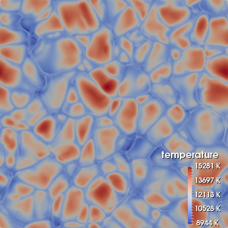
Figure 1: Temperature field for a horizontal cut where the horizontally averaged temperature $\langle T\rangle\approx{\rm T_{\rm eff}}$, at 912 m below the top of the simulation box, for a snapshot of our 3D simulation.

Our starting model has $T_{\rm eff}=11800$ K, a gravitational acceleration of $\rm\log(g)=8$, and a pure hydrogen composition. Vertical extent and numerical resolution are determined by the effective height of the convective zone including the overshooting region and by requiring a well-resolved thermal structure. The horizontal directions scale with an aspect ratio of $\rm 2.2$ and allow for $\gtrsim 6\text{--}8$ granules in each direction. A vertical resolution of $\sim 15$ grid cells per pressure scale height $H_{\rm p}$ ensures an average change of pressure $\lesssim 7\%$. For a total vertical extent of $\sim 16.8\,H_{\rm p}$, $\rm 252$ cells are used vertically while $\rm 522\times 522$ cells are used horizontally, with grid spacings $\rm\Delta x=29.42\,m$ vertically and $\rm\Delta y=\Delta z=31.19\,m$ horizontally. The simulated box thus has a volume of $\rm 7.384\times 16.28\times 16.28\,{\rm km}^{3}$ and consists of about $6.8\cdot 10^{7}$ grid cells. A snapshot from this simulation is shown in Fig. 1.

We use the time a sound wave requires to travel from top to bottom as a unit here, whence $\rm\tau_{scrt}=0.236\,sec$. The simulation has been run for $\rm 92\,scrt$, i.e., $\rm 21.7\,sec$, resulting in $\rm 2\,TB$ of data. This includes $t_{\rm 2D}=\rm 30\,scrt$ of initial relaxation of the mean structure by a 2D simulation with otherwise identical extent, resolution, and physical parameters. The 2D simulation was started from a 1D model computed with the Warsaw envelope code (Paczyński, 1969, 1970; Pamyatnykh, 1999) and saves relaxation time for the mean stratification in the overshooting zone which cannot be accurately guessed from our 1D model. The transfer from 2D to 3D was established by horizontally averaging a snapshot of the 2D simulation to generate a new, ‘pre-relaxed 1D model’ which was then used as initial condition for the 3D simulation. The time $t_{\rm 2D}$ was chosen to ensure zero total vertical momentum at a time where strong vortices in the overshooting zone have not yet developed. The pre-relaxed 1D model was then perturbed again as described above. The statistical analysis is based on snapshots of density, momentum, internal energy, radiative flux, and pressure made each $\rm 0.1\,scrt$. Further quantities of interest can be calculated in post-processing, e.g., mean values (horizontally and also in time), variance, skewness, kurtosis, and cross correlations of various fields. The statistical analysis has been performed from averages over the last $t_{\rm stat}\sim\rm 22\,scrt$ of the simulation.

3 Mean structure, relaxation, and velocities

3.1 Mean structure

In Fig. 2 we compare $\nabla_{\rm ad}-\nabla$ of the simulation averages with results from a 1D stellar model with ML2 convection model (Böhm & Cassinelli, 1971) using $\alpha=0.67$, where $\alpha$ has been adjusted to provide the best fit to the final state of the 3D simulation. We observe that the simulation averages and the 1D model merge towards the interior, below layers where $\log(1-M_{r}/M_{\star})\gtrsim-13.5$. Above that layer differences in the gradients occur due to overshooting modifying the stratification, i.e.  where $-13.5\gtrsim\log(1-M_{r}/M_{\star})\gtrsim-15$. The superadiabatic feature at $\log(1-M_{r}/M_{\star})\approx-16.4$ is slightly broader and shallower in the simulation than it is for the stellar model. Differences further above it are due to the different treatment of radiative transfer and the upper boundary conditions in the simulation and the 1D model.

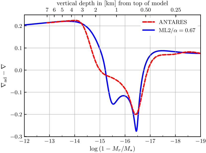
Figure 2: Adiabatic minus average temperature gradient from the numerical simulation (ANTARES) and a 1D model based on the ML2 mixing length model with an $\alpha$–parameter of $0.67$.

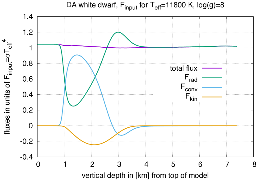
Figure 3: Radiative, convective, and kinetic energy fluxes, denoted as $F_{\rm rad}$, $F_{\rm conv}$, and $F_{\rm kin}$, as well as their sum $F_{\rm total}$, each normalised relative to the input flux of the 1D starting model, plotted against depth measured from the top of the simulation box.

In Fig. 3 we compare the contributions of radiative, convective, and kinetic energy fluxes in the vertical direction to the total (vertical) energy flux. The Schwarzschild unstable region ranges from 0.8 km down to 2 km (as measured from the top of the simulation box). This is followed by a large overshooting region with non-zero convective and kinetic energy fluxes. The latter essentially vanish around 4 km.

3.2 Relaxation

We discuss in more detail the relaxation process during our 3D simulation and the accuracy which we can expect for our statistical data averaged over $t_{\rm stat}$. Already from the total energy flux depicted in Fig. 3, which is obtained from averaging the horizontal average of $F_{\rm total}$ over $t_{\rm stat}$, we can expect the simulation to be quite close to thermal relaxation, since the deviations of $F_{\rm total}$ from $F_{\rm input}$ are about $4\%$ or less. In Kupka & Muthsam (2017) it is explained in detail why we can expect a simulation to require thermal relaxation only for the upper part of the simulation domain, if it is started from an initial condition where the lower part of the computational domain — located more closely to the stellar interior — is already in a (nearly) relaxed state. This is possible if the lower part is either stratified quasi-adiabatically as in simulations of solar granulation or radiatively as in the present case, since both can easily and sufficiently accurately be guessed from a 1D model. Indeed, for the solar case fast relaxation from various initial conditions, all quasi-adiabatic for the solar interior, was demonstrated with ANTARES by Grimm-Strele et al. (2015a) (see their Fig. 9 and 10).

However, there is a region in the DA white dwarf considered here, for which the thermal structure cannot be easily guessed from a 1D model: the region of overshooting below the convection zone. There, $F_{\rm rad}$ is up to 20% larger than the total flux (see Fig. 3). These layers require thermal relaxation and thus enforce a minimum relaxation time much larger than in surface convection simulations of stars with a lower boundary placed inside a quasi-adiabatic convection zone such as that one of our Sun (cf. Kupka & Muthsam 2017).

In many cases of astrophysical interest the thermal relaxation time associated with a certain layer of a star is approximately equal to the Kelvin-Helmholtz time scale for that layer (cf. Chap. 2.3.4 in Kupka & Muthsam 2017 and also Chap. 5 and 6 in Kippenhahn & Weigert 1994, also for discussions of limitations of applicability of this approximation): $t_{\rm therm}(x)\approx t_{\rm KH}(x)$. The latter is obtained from integrating $t_{\rm KH}(x)\equiv-3(\int_{a}^{b}p\rho^{-1}dM_{s})/L_{r}$, where $a$ is the mass near the surface of the star (or the simulation box, here $\approx 0$) and $b$ is the mass contained above that layer at depth $x$, i.e., $M_{s}$. We recall that $p$ and $\rho$ are pressure and density, whereas $L_{r}=4\pi r^{2}F_{\rm total}$ is the local luminosity. It is straightforward to adopt this to a box-in-a-star configuration with plane parallel geometry and obtain a practical definition for $t_{\rm KH}(x)$, namely: $t_{\rm KH}(x)\equiv\langle\,3(\int_{0}^{x}p(x^{\prime})dx^{\prime})/F_{\rm total}\,\rangle_{\rm h,t}$, where the integration occurs over vertical location $x^{\prime}$, with $0\leqslant x^{\prime}\leqslant x$, and the result is averaged horizontally and in time — or a horizontally averaged pressure is time averaged, as we have done here. In Fig. 4 we plot this calculation of $t_{\rm KH}(x)$ for our simulation as a function of depth along with the acoustic time $t_{\rm ac}(x)$, i.e., the time a sound wave requires to travel from the top of a simulation box to a particular layer at the vertical point $x$. In addition, we display the convective time scale $t_{\rm conv}(x)$, which is likewise obtained from integrating the inverse of the time and horizontally averaged root mean square of the fluctuating part of the vertical velocity, i.e., the square root of $w^{2}_{\rm rms}=\langle(w-\langle w\rangle_{\rm h})^{2}\rangle_{\rm h,t}=\langle w^{\prime 2}\rangle_{\rm h,t}$, from top down to $x$. Clearly, $\tau_{\rm scrt}=t_{\rm ac}(x_{\rm bottom})$. Now before statistics can be collected (i.e., ahead of averaging results over the statistical sampling time $t_{\rm stat}$), the time integration has to be first performed long enough such that initial perturbations both of the thermal mean structure (given by $p$, $T$, $\rho$) and the velocity field no longer influence the result and this is just the relaxation time scale $t_{\rm relax}$. Following the discussion on thermal relaxation in Kippenhahn & Weigert (1994) and on relaxation of hydrodynamical simulations of stellar convection in Kupka & Muthsam (2017) we can expect $t_{\rm relax}=\max(t_{\rm KH}(x_{1}),t_{\rm conv}(x_{2}))$, i.e., the maximum of $t_{\rm KH}(x_{1})$, evaluated at a layer $x_{1}$ below which the stratification is essentially in thermal equilibrium already from the beginning, and of $t_{\rm conv}(x_{2})$, where $x_{2}$ is evaluated close to the bottom of the simulation domain (or at the bottom in case of open boundary conditions). We find $F_{\rm total}\approx F_{\rm rad}$ below $x_{1}=4$ km throughout most of our simulation. Precisely, their difference drops strictly monotonically from $\sim 0.8\%$ at 4 km to $\lesssim 0.1\%$ at 5.5 km, and $\lesssim 0.01\%$ at 7 km. In the same region, $F_{\rm total}$ differs from $F_{\rm input}$ on average by $\lesssim 1.5\%$ and at most by $<2.3\%$. We choose $x_{2}$ slightly above $x_{\rm bottom}$ to avoid the layers where $w^{2}_{\rm rms}\rightarrow 0$. We conclude that $t_{\rm KH}(x_{1})\approx 25~{}{\rm s}\approx 106\,\tau_{\rm scrt}$ and $t_{\rm conv}(x_{2})\approx t_{\rm conv}(x=7\,{\rm km})\approx 30~{}{\rm s}\approx 127\,\tau_{\rm scrt}$. So we expect the relaxation of the thermal stratification and the velocity field to require up to roughly $130\,\tau_{\rm scrt}$.

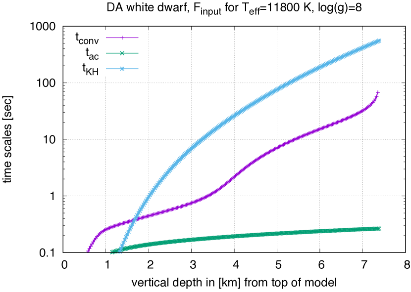
Figure 4: Integral time scales of interest for relaxation computed here as a function of model depth: the convective turnover time $t_{\rm conv}$, acoustic time $t_{\rm ac}$, and Kelvin-Helmholtz time $t_{\rm KH}$.

To show the degree of thermal relaxation and the simulation time required to achieve it we evaluate $F_{\rm rad}$ at the top of the simulation box to plot it against model age measured in $t_{\rm scrt}=t/\tau_{\rm scrt}$ where $t$ is the model age in seconds. We note that until $t_{\rm scrt}=30$ the simulation has been evolved in 2D and has then been reset through horizontally averaging that state to provide the initial condition of the 3D simulation, as described in Sect. 2. For a thermally relaxed model we expect $F_{\rm rad}(x_{\rm top})\approx F_{\rm input}$. In Fig. 5 we see the result for our simulation from the beginning of the 3D setting. During the first 20 scrt there is obviously some major readjustment going on until a convergence of $F_{\rm rad}(x_{\rm top})\rightarrow F_{\rm input}$ sets in which is roughly proportional to ${t_{\rm scrt}}^{-1/2}$ during the time over which we have performed the simulation (halving the flux difference with respect to $F_{\rm input}$ requires to continue the simulation for twice the amount of time). We have decided to also drop the next segment of 20 scrt for statistical evaluation and begin with the computation of $t_{\rm stat}$ at $t_{\rm scrt}\approx 70$.

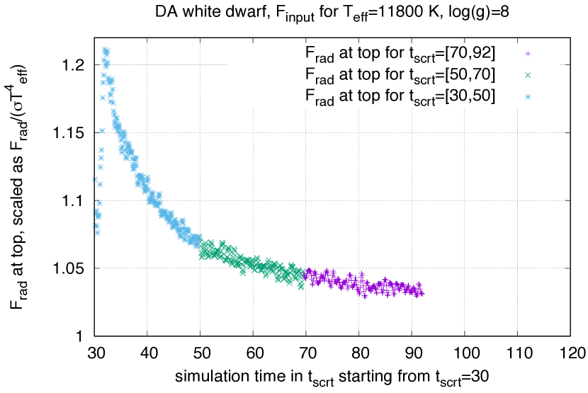
Figure 5: Thermal relaxation is shown here by the time evolution of the emerging radiative flux at the top of the simulation, normalised by the input flux, plotted as a function of model age $t_{\rm scrt}$, and grouped into three consecutive sets of data.

Averaged over the time interval of $t_{\rm stat}$, we find an emerging radiative flux $F_{\rm rad}(x_{\rm top})/F_{\rm input}\approx 1.03845$, when normalizing it relative to $F_{\rm input}$. This corresponds to a $T_{\rm eff}$ of 11912 K and may be compared with an equivalent of 12197 K obtained when averaging over the first $\rm 10\,scrt$ of the 3D simulation, at the beginning of relaxation. For the average over the last $\rm 5\,scrt$ of $t_{\rm stat}$ we find $F_{\rm rad}(x_{\rm top})/F_{\rm input}$ to have dropped already below $1.035$, whence $T_{\rm eff}\approx 11900$ K. From the time dependence seen in Fig. 5 we expect that a doubling of simulation time from $t_{\rm scrt}=30$ onwards, i.e., up to $t_{\rm scrt}\approx 154$, would allow halving the residual flux difference to less than $2\%$ and thus $T_{\rm eff}\lesssim 11850$ K, in agreement with the relaxation estimate discussed above for $t_{\rm KH}$ (see Fig. 4). We note that from an observer’s point of view we might use the emitted surface flux, i.e. a $T_{\rm eff}$ of 11912 K, to characterize the simulation when averaging it from a $t_{\rm scrt}$ of 70 to 92. However, for the present discussion we prefer to use the input flux at the bottom (equivalent to $T_{\rm eff}=11800$ K) for scaling the results, since this value is fixed throughout the simulation.

The differences between surface and input radiative flux which are expected to remain at that value of $t_{\rm scrt}$ are partially caused by the initial stratification of the lower region not being in perfect thermal equilibrium, in particular with respect to its interaction with layers further above. But there are also systematic differences introduced by numerical inaccuracies of the radiative transfer solver (cf. the little in dip in $F_{\rm total}$ around a depth of 1 km in Fig. 3 — we point out here that this quantity is not often shown in publications on numerical simulations of stellar surface convection, but when it is, similar features are found for layers near the stellar surface). Other sources of systematic differences of similar order or smaller occur when comparing grey with non-grey radiative transfer (cf. Grimm-Strele et al. 2015a and also Tremblay et al. 2011), or they originate from the detailed implementation of the input boundary condition as well as from differences between the numerical approximation and assumed microphysics of the 1D starting model in comparison with the numerical simulation. Although one could try to “remove” residual flux differences originating from these sources by longer relaxation, it makes neither physical nor mathematical sense to do so: the systematic and numerical errors they contribute to are already roughly equal to the flux difference caused by an “incomplete relaxation” of the order of 2% of the total flux. For the same reason it is also not important whether we estimate $t_{\rm KH}(x)$ by averaging over $t_{\rm stat}$, as we have done, or calculate it from the initial condition to guide the simulation. An estimate of the numerical errors due to resolution on the mean temperature profile as obtained from numerical simulations of solar granulation with ANTARES has been made by Grimm-Strele et al. (2015b): the accumulated error over several sound crossing times — for a relative resolution roughly comparable to the one used in the present work — was found in the range of a fraction of one percent, with maximum errors up to a few percent. The error calculated that way is chiefly due to finite resolution in the numerical simulation and since the relative resolutions, maximum Mach numbers, etc., are roughly comparable to our present case, we should expect relative (numerical) errors of similar size also for the present simulation. Moreover, from Fig. 5 we can see the impact of oscillations present in the simulations: they lead to a variation in $F_{\rm rad}(x_{\rm top})/F_{\rm input}$ of $\pm 0.5\%$ over $\tau_{\rm scrt}$ (we discuss those further below).

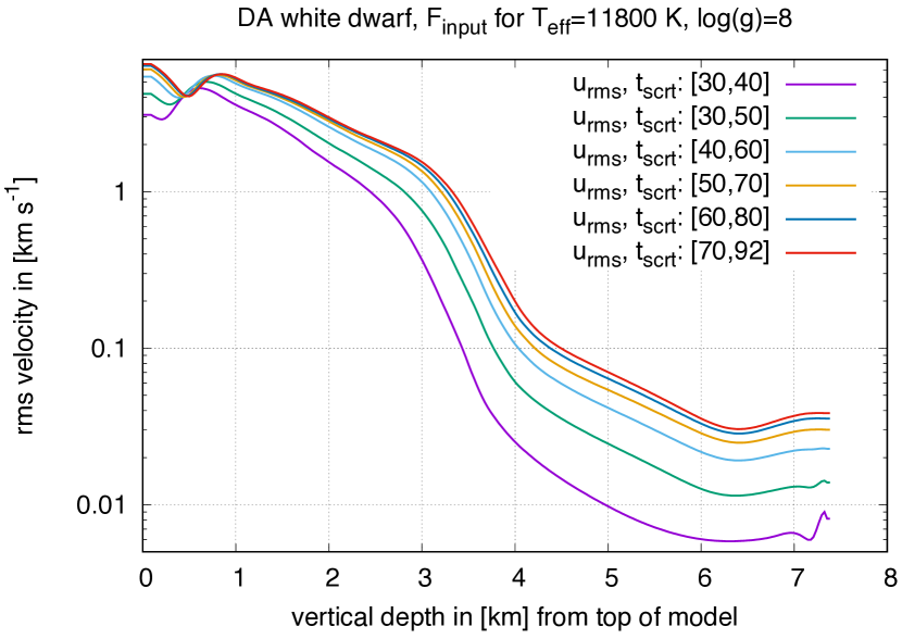
Figure 6: Relaxation of the root mean square average of the fluctuation of the $u$-component of horizontal velocity around its horizontal mean, $u_{\rm rms}$, displayed as a function of depth and time averaged over a sequence of intervals distinguished by model age $t_{\rm scrt}$.

It is thus of little practical use to extend the present simulation over a longer interval in time. If at all, one may consider $t_{\rm scrt}\rightarrow 150$, since beyond this value the systematic errors become dominant. But as we show here, also for sufficiently accurate statistics of the velocity field time integration beyond $t_{\rm scrt}\approx 92$ is not necessary. Fig. 6 provides an example for the rapid convergence of the velocity field towards a statistically stationary state well within our estimate of $t_{\rm conv}(x_{2})$ discussed along Fig. 4. We find halving of the relative error of the horizontally and time averaged root mean square of the fluctuation of the $u$-component of horizontal velocity, $u_{\rm rms}$, relative to its instantaneous horizontal mean for each consecutive interval of 10 scrt, i.e., $\propto{t_{\rm scrt}}^{-2}$. As can be estimated from the mere $12\%$ increase through most of the layers of the simulation when progressing from a $t_{\rm scrt}$ in the interval $[60,80]$ to $[70,92]$, i.e. the range of $t_{\rm stat}$, quadratic convergence is found for nearly the entire simulation duration of $t_{\rm scrt}$. This is fast enough such that the difference between these two averagings is already the entire expected growth if the computation were continued beyond a $t_{\rm scrt}$ of about 150. Fig. 6 thus also provides an error estimate for $u_{\rm rms}$ with respect to its relaxation.

For the surface layers this error is even much smaller and clearly it converges rapidly throughout the entire simulation box. This similarly holds for the siblings of $u_{\rm rms}$, i.e., $v_{\rm rms}$ and $w_{\rm rms}$, which characterise the second horizontal and the vertical component of the flow. Also skewness and kurtosis of velocity and temperature fields, i.e., higher-order statistical correlations that we discuss below in Sect. 4.2, converge fast but for a limited region dominated by single events which is explained there in more detail. We can hence safely use velocity and temperature statistics averaged over $t_{\rm scrt}$ in the following discussion. From a physical point of view this fast convergence of the statistics for the velocity field irrespectively of the less accurate convergence of the emerging radiative flux is not surprising: the velocity fields are generated by convective processes occurring in the upper part of the simulation box (with very short relaxation times). All what is left is a small drift as a function of time, which does not affect the functional form, physical processes, and even the level of accuracy we expect from the velocity related quantities that we discuss below. The independence of the residual error in the velocity field from the degree of thermal relaxation is also corroborated by the completely different convergence rates, $\propto{t_{\rm scrt}}^{-2}$ for $u_{\rm rms}$ and $\propto{t_{\rm scrt}}^{-1/2}$ for the total (radiative) flux at the surface. We expect the faster convergence rate of velocities to change to the smaller one of thermal relaxation once $t_{\rm scrt}\gtrsim t_{\rm conv}(x_{2})/\tau_{\rm scrt}\approx 127$. As discussed in the context of thermal relaxation, at this point in time evolution the model intrinsic errors dominate over the residual error, and the accuracy reached for $u_{\rm rms}$ and related quantities at $t_{\rm scrt}\in[70,92]$ is already adequately small. Thus, our simulation data obtained over $t_{\rm stat}$ are both based on a sufficiently well relaxed simulation and have statistical errors small enough to be useful subsequently.

3.3 Velocities

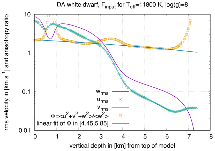
Figure 7: Vertical rms velocity, $w_{\rm rms}$, and its horizontal counterparts, $u_{\rm rms}$ and $v_{\rm rms}$, perfectly agreeing, on a logarithmic scale. The dimensionless anisotropy ratio $\Phi$ is also plotted together with its linear fit computed for the interval from 4.45 km to 5.85 km.

As the vertical and horizontal velocity fields are reasonably well converged in the convection zone and in the overshooting region underneath, we can analyse the time and horizontally averaged root mean square of their fluctuating components, i.e., $w_{\rm rms}$ for the vertical velocity, and likewise $u_{\rm rms}$ and $v_{\rm rms}$ for the two horizontal components. In Fig. 7 we plot them on a logarithmic scale. From local maxima of $\sim 5.7~{}{\rm km\,s}^{-1}$ near the top of the convective zone they gradually drop towards its bottom. Where $F_{\rm conv}$ changes sign (see Fig. 3), $u_{\rm rms}$ and $v_{\rm rms}$ have reached $\sim 1.8~{}{\rm km\,s}^{-1}$ while $w_{\rm rms}$ is still $\sim 2.8~{}{\rm km\,s}^{-1}$, but has begun to decay much faster, a process occurring for $u_{\rm rms}$ and $v_{\rm rms}$ again from around 3.2 km onwards. The horizontal velocity components begin to dominate the total kinetic energy and $\Phi=(w_{\rm rms}^{2}+u_{\rm rms}^{2}+v_{\rm rms}^{2})/w_{\rm rms}^{2}$ exceeds a value of 2 with a local maximum around 3.5 km. There, a rapid, exponential decay sets in. It is slightly larger for $u_{\rm rms}$ and $v_{\rm rms}$. For $w_{\rm rms}$ the decay slows down around 4 km, where $F_{\rm conv}$ begins to vanish ($-1\%\lesssim\,F_{\rm conv}/F_{\rm input}\lesssim\,0\%$). The decay of $u_{\rm rms}$ and $v_{\rm rms}$ continues to be rapid down to about 4.2 km and $\Phi<2$. The simulation can be used for an accurate study of even deeper layers where the lower boundary is still sufficiently away to avoid direct interference. We find that velocities decay at a slower rate than in the “overshooting zone proper". Interestingly, $u_{\rm rms}$ and $v_{\rm rms}$ continue to decay more rapidly than $w_{\rm rms}$: over an extended region from about 4.45 km to 5.85 km $\Phi$ features a nearly linear decrease with depth which ceases only once the influence of the lower (closed) boundary condition becomes notable. Fig. 7 highlights this relation by a linear least squares fit of $\Phi$ for that region. Note that the logarithmic scale in that figure would actually suggest an exponential fit for $\Phi$ while a plot in linear scale motivates the linear model function chosen. This small difference is caused by a very low e-folding scale: in this case an actually exponential function can be approximated by a linear function over an extended range. We return to a comparison between both models in Sect. 4.3.2.

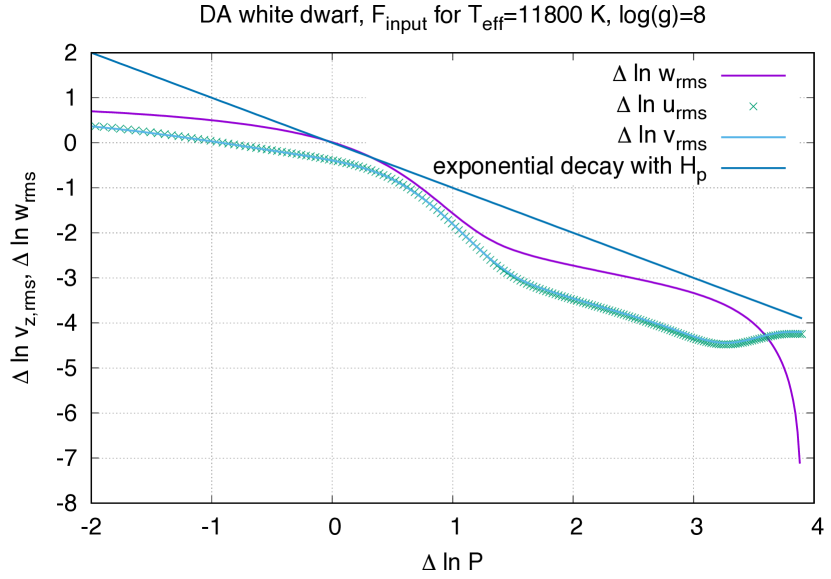
Figure 8: Logarithm of $w_{\rm rms}$, $u_{\rm rms}$, and $v_{\rm rms}$, as functions of the logarithm of total pressure, relative to a reference velocity and pressure. The exponential decay hypothesis for $w_{\rm rms}$ as function of pressure scale height is indicated.

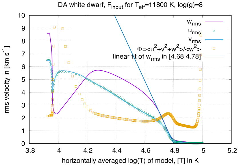
Figure 9: $\Phi$ as well as $w_{\rm rms}$, $u_{\rm rms}$, and $v_{\rm rms}$ as functions of $\log T$ alongside a linear fit of $w_{\rm rms}$ in the overshooting region (see text).

In Fig. 8 we plot the logarithm of $w_{\rm rms}$ as well as $u_{\rm rms}$ and $v_{\rm rms}$ as functions of $\ln\,P$, normalised relative to the velocity and the total pressure at the layer where $F_{\rm conv}$ changes sign (at 2.785 km in Fig. 3). We also plot a line to indicate an exponential decay of the vertical velocity field with $H_{\rm p}$, as proposed in Tremblay et al. (2015) to occur for DA WDs. We cannot identify a unique exponential scaling law for $w_{\rm rms}$ in regions where $F_{\rm conv}<0$. For the layers where $\Delta\ln P$ is between 0 and 1.5 ($|F_{\rm conv}/F_{\rm input}|>1\%$), the decay rate is first about $1\,H_{\rm p}$, then becomes twice as steep $(0.5\,H_{\rm p})$, then settles at a quarter of that rate $(2\,H_{\rm p})$. Similar holds for $u_{\rm rms}$ and $v_{\rm rms}$ with a shift in location and different decay rates particularly for $\Delta\ln P\gtrsim 1.5$. No simple polynomial law can describe this dependency either (Canuto & Dubovikov 1997 derived a polynomial decay as function of distance from the convection zone if the dissipation rate of turbulent kinetic energy were computed from its local limit expression, cf. Fig. 7).

In turn, $w_{\rm rms}$ depends linearly on $\log T$ from 2.73 km, where $F_{\rm conv}\gtrsim 0$, down to about 3.73 km, where $F_{\rm conv}/F_{\rm input}\approx-2\%$ (see Fig. 9). The linear fit of $w_{\rm rms}$ as a function of $\log T$ finds $w_{\rm rms}$ to become zero where $F_{\rm conv}/F_{\rm input}\approx-0.87\%$, although this occurs below the domain of its validity. There, $\log T\approx 4.80$ at a depth of $\approx 3.97$ km. Inside the fit region, $\Delta\ln P$ increases from $-0.07$ to $1.04$. A linear decay of $w_{\rm rms}$ as a function of $\log T$ for exactly the same part of the overshooting region has been reported by Montgomery & Kupka (2004) for hotter DA WDs with $T_{\rm eff}\gtrsim 12200$ K when solving the Reynolds stress model of Canuto & Dubovikov (1998). Note that the same scaling could also be inferred from Fig. 4 of Tremblay et al. (2015) for their models with a $T_{\rm eff}$ of 12100 K, 12500 K, and, roughly, also 13000 K for “zone 3" (cf. their Table 1). As hydrogen is fully ionised in that zone and $F_{\rm total}\approx F_{\rm rad}$, both $T$ and $H_{\rm p}$ scale linearly with depth, thus our Fig. 9 and Fig. 1 of Montgomery & Kupka (2004) imply the same (non-) linear decay of $w_{\rm rms}$ with $T$ and $H_{\rm p}$, albeit (cf. Fig. 8) this also only holds for a limited region.

4 Analysis

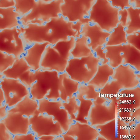
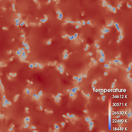
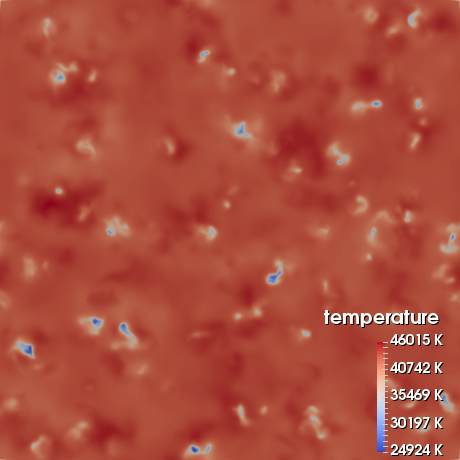
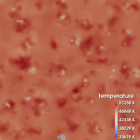
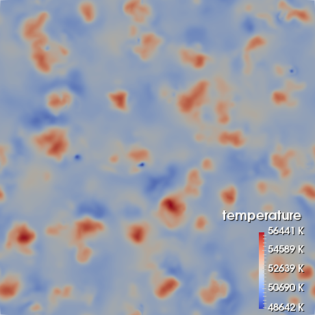
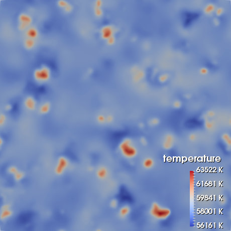
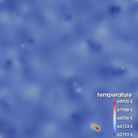
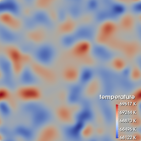
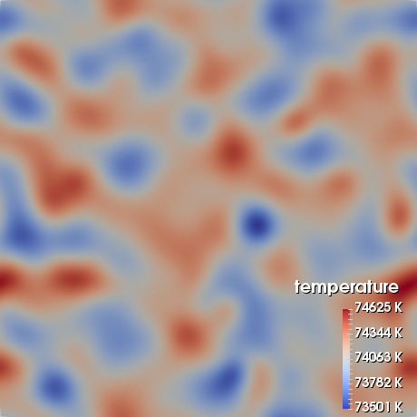
Figure 10: Horizontal cuts of temperature as a function of depth at time $t_{\rm scrt}=92$. The top row displays snapshots at depths of 1.50 km, 2.00 km and 2.50 km (Fig. 10a–c) as measured from the top of the simulation box. The middle row continues this series for depths of 2.75 km, 3.00 km and 3.50 km (Fig. 10d–f). The bottom row displays the cuts for depths of 4.00 km, 4.50 km and 5.00 km (Fig. 10g–i). Note that the temperature scale changes for each snapshot and the ratio between maximum and minimum value peaks near the Schwarzschild stability boundary around 2.00 km. Clearly inside the plume-dominated region it is already smaller and drops only gently from 3.00 km to 4.00 km. There is again a drastic drop in scale for layers inside the wave-dominated region.

4.1 The temperature field and overshooting

One may characterise an overshooting zone with respect to the sign of the convective flux, the superadiabatic gradient (or alternatively the gradients of entropy or potential temperature), the flux of (turbulent) kinetic energy, the mass flux, or the local maxima and minima of these quantities. Assuming a nearly adiabatic temperature gradient for cases of convection at low radiative loss rates (high Peclet number) Zahn (1991) distinguished a separation of the Schwarzschild unstable convection zone proper ($F_{\rm conv}>0$, $\nabla>\nabla_{\rm ad}$, with $|\nabla-\nabla_{\rm ad}|/\nabla_{\rm ad}\ll 1$), from the zone of subadiabatic penetration ($F_{\rm conv}<0$, $\nabla<\nabla_{\rm ad}$, while again $|\nabla-\nabla_{\rm ad}|/\nabla_{\rm ad}\ll 1$), and the thermal boundary layer ($F_{\rm conv}<0$, $\nabla<\nabla_{\rm ad}$, but $|\nabla-\nabla_{\rm ad}|/\nabla_{\rm ad}\rightarrow O(1)$), until eventually $F_{\rm conv}\approx 0$ (stable, radiative region, no longer mixed by convection). This case of penetrative convection he distinguished from the case of overshooting for which a more narrow definition was suggested: there, large radiative losses prevent altering the temperature gradient towards the adiabatic one in regions where $F_{\rm conv}<0$.

For the DA white dwarf we consider in the present case, it follows from Fig. 3 that radiative losses everywhere in the overshooting region are large (low Peclet number). So it makes sense to distinguish, as in Freytag et al. (1996), the following regions. First of all, the convection zone proper with its Schwarzschild boundary ($F_{\rm conv}>0$, $\nabla>\nabla_{\rm ad}$) and then an overshooting region where plumes gradually heat up that do not yet experience negative net buoyancy (and which we call countergradient region, $F_{\rm conv}>0$, $\nabla<\nabla_{\rm ad}$). The layer at which the change of sign in $F_{\rm conv}$ occurs is termed “flux boundary” by some authors, for example, in Tremblay et al. (2015). From there onwards throughout where $F_{\rm conv}<0$ and $\nabla<\nabla_{\rm ad}$, plumes penetrate into a region of counterbuoyancy. We call this the plume-dominated region in the following. One might also consider the local minimum of $F_{\rm conv}$ to mark the region where the thermal boundary layer begins, as in Zahn (1991), although this has a less important role, as we see in the following figures. Finally, motion can persist beyond where $F_{\rm conv}\rightarrow 0$ and $\nabla<\nabla_{\rm ad}$, which we further below call the wave-dominated region. The reasons for this naming become evident from the following figures.

In Fig. 10a, well inside the convection zone, the network of intergranular lanes is still clearly visible, similar to the stellar surface depicted in Fig. 1, although the temperature contrast between maximum and minimum values has become larger and more skewed (low temperature regions cover a smaller area). At the Schwarzschild boundary, Fig. 10b, the granular structure is still recognizable, but the intergranular “network” of downflows is no longer connected; rather, it is characterised by plumes, chiefly grouped together near corner points where several granules meet each other in layers inside the convection zone. The now isolated, cold downflow columns maintain their identity (Fig. 10c), although they gradually lose the contrast between them and their environment, until the “flux boundary” is reached, where $F_{\rm conv}$ changes sign (Fig. 10d). Below this level the structure rapidly changes: the temperature contrast is drastically reduced over a small distance, from $3:2$ at the flux boundary around 2.75 km to just $7:6$ at 3.00 km (Fig. 10e). Now the plumes have reverted their role: they are hotter than their environment. This structure is maintained throughout the entire plume-dominated region (Fig. 10e–g). The contrast drops only gently (down to $9:8$), but more importantly, the number of plumes per area and the area each of them covers rapidly decrease. Indeed, at 4.00 km we see just one strong plume left in comparison with some three dozen at 3.00 km. As we know through Fig. 3, around 4.00 km, $F_{\rm conv}/F_{\rm total}\rightarrow 0$ (essentially), and a new pattern becomes visible. This pattern remains throughout the wave-dominated region depicted in Fig. 10h–i, with the small contrast between maximum and minimum temperature slowly decreasing from 2.2% to 1.5%. This continues further into the wave–dominated region (e.g., to a contrast of 1.2% at 5.50 km, not shown in Fig. 10), although the visible structures have no longer the trivial vertical correlation which is easily found for the layers further above. We remark here that the flow patterns — which allow an easy distinction between the convectively unstable, the counter–gradient, the plume–dominated and the wave–dominated region — are present already at $t_{\rm scrt}=35$. They are not related to the patterns of initial relaxation, say at $t_{\rm scrt}=30.1$, where the wave–dominated region is still mostly unperturbed ($\Delta T<1\,{\rm K}$ at 5.00 km) and the pattern visible in the plume–dominated region has very little, if any, relation to what can be seen in the wave–dominated region 5 scrt later. We conclude that the patterns observed in Fig. 10 are intrinsic to the flow, but not to the initial perturbation chosen to start it, either in the wave–dominated region, or in any layer further above. We skip a similarly detailed discussion of the velocity field and instead demonstrate how skewness and kurtosis capture many of the statistical and topological properties of the velocity and temperature field.

4.2 Skewness and kurtosis of velocity fields and temperature

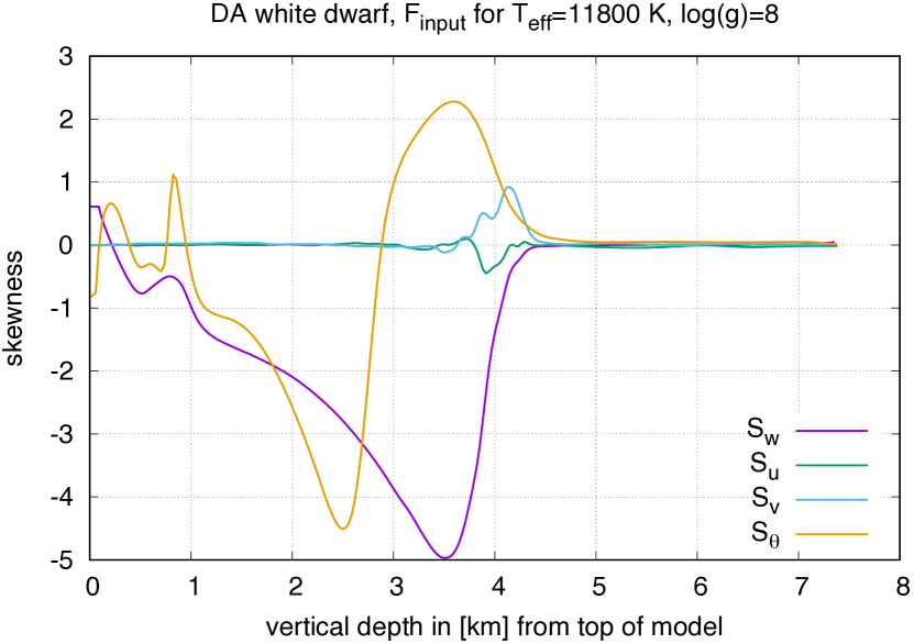
Figure 11: Skewness of fluctuations of the temperature field, $S_{\theta}$, and the components of the velocity field, $S_{w},S_{u},S_{v}$, around their horizontal mean, averaged over each layer and in time (over $t_{\rm stat}$), plotted as a function of depth.

In Fig. 11 we display the skewness of fluctuations of the temperature field, $S_{\theta}$, and the vertical ($w$) and horizontal components of the velocity field, $S_{w}$, $S_{u}$, and $S_{v}$, around their horizontal mean, averaged over each layer and in time (over $t_{\rm stat}$), plotted as a function of depth. The negative values of $S_{\theta}=\langle(T-\langle T\rangle_{\rm h})^{3}\rangle_{\rm h,t}/(\langle(T-\langle T\rangle_{\rm h})^{2}\rangle_{\rm h,t})^{3/2}=\langle T^{\prime 3}\rangle_{\rm h,t}/(\langle T^{\prime 2}\rangle_{\rm h,t})^{3/2}$ within the convectively unstable zone indicate that locally low values of $T$ cover a smaller surface area and hence have to deviate further from the horizontal mean value than locally high values, in perfect agreement with Fig. 10a. Within the countergradient region this becomes even more pronounced due to the fast columns of downflows generated by the strongest remnants of the downflow network (cf. Fig. 10c). The situation becomes reversed around the flux boundary (Fig. 10d) and the plumes, which cover a smaller area than the upflow, are now hotter than their environment (Fig. 10e–f). Hence, $S_{\theta}>0$ in that region with a pronounced global maximum where $S_{w}$ has its global minimum. Eventually, in the wave-dominated region, $S_{\theta}\rightarrow 0$ which demonstrates that the temperature distribution is symmetric around its horizontal mean in those layers. In comparison, $S_{w}$, which is defined analogously to $S_{\theta}$, but for the vertical velocity field, also demonstrates that the downflows cover a more narrow area than the upflows (due to conservation of mass and momentum), whence $S_{w}<0$ in the convection zone. The distribution becomes more and more skewed once the network of downflows has transformed into a set of plumes where only the fastest and hottest one can penetrate sufficiently deep (cf. Fig. 10f and note its location close to the global extrema of $S_{w}$ and $S_{\theta}$). Once the plumes disappear in number, $S_{w}\rightarrow 0$ and remains near that value for the entire wave-dominated region. Since the simulation has (or, rather, should have) no preferred symmetry of velocities into any of the horizontal directions, we expect $S_{u}\approx 0$ and $S_{v}\approx 0$ throughout the simulation and this is also an indicator for the degree of convergence of the statistical results. We find this confirmed by Fig. 11 with one exception: around 4 km, both $S_{u}$ and $S_{v}$ deviate from $0$ and this can be understood as resulting from the statistics depending on very few events with large impact, i.e., on a few plumes managing to penetrate deep enough (Fig. 10g), leading eventually to sidewards flow by conservation of mass. Many more such events are required to obtain a converged statistical result within $t_{\rm stat}$ in that region at the given horizontal extent of our simulation.

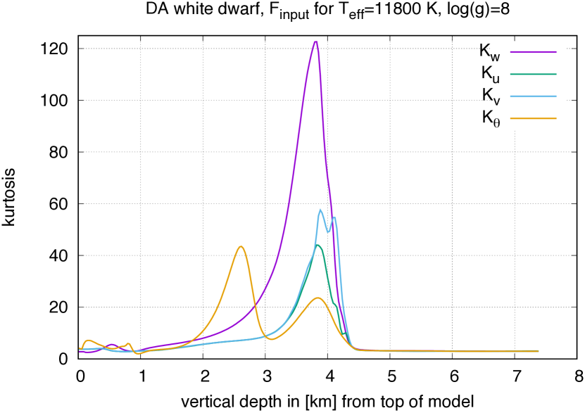
Figure 12: Kurtosis of fluctuations of the temperature field, $K_{\theta}$, and the components of the velocity field, $K_{w},K_{u},K_{v}$, around their horizontal mean, averaged over each layer and in time (over $t_{\rm stat}$), plotted as a function of depth (full range of kurtosis shown).

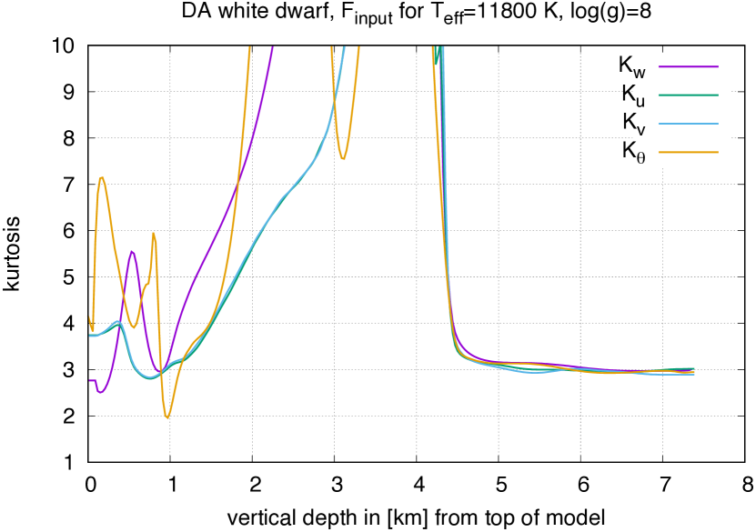
Figure 13: Kurtosis of fluctuations of the temperature field, $K_{\theta}$, and the components of the velocity field, $K_{w},K_{u},K_{v}$, around their horizontal mean, averaged over each layer and in time (over $t_{\rm stat}$), plotted as a function of depth (values truncated above 10).

In Fig. 12 we display the kurtosis of fluctuations of the temperature field, $K_{\theta}$, and the vertical and horizontal components of the velocity field, $K_{w}$, $K_{u}$, and $K_{v}$, computed in analogy to skewness except that now $K_{\theta}=\langle(T-\langle T\rangle_{\rm h})^{4}\rangle_{\rm h,t}/(\langle(T-\langle T\rangle_{\rm h})^{2}\rangle_{\rm h,t})^{2}=\langle T^{\prime 4}\rangle_{\rm h,t}/(\langle T^{\prime 2}\rangle_{\rm h,t})^{2}$, and likewise for the components of the velocity field. The kurtosis provides a measure of the strength and importance of deviations of a fluctuation from a given root mean square average. For a mathematically meaningful distribution, $K\geqslant 1$. For a Gaussian distribution, $K=3$ in addition to $S=0$. These are necessary though not sufficient conditions for Gaussianity. As one can read from Fig. 12 the plumes lead to extreme values of $K_{w}$, especially where a few, isolated plumes dominate the distribution (around 4 km). In comparison, for $K_{\theta}$ the flux boundary with its reversion from cold to hot plumes leads to a local minimum in that region (around 3 km). For the Sun or other main sequence stars (Kupka & Robinson 2007; Kupka 2009) the network of downflows with its embedded granules leads to global minima of $K_{\theta}$ and $K_{w}$ at the superadiabatic peak and we find this also for our simulation of a DA white dwarf (neglecting the top of the simulation box) (see Fig. 13). Likewise, for both $K_{\theta}$ and $K_{w}$ the plumes in the overshooting region lead to very large values of K which characterises their large deviation from the root mean square values of fluctuations of vertical velocity and temperature. In the wave-dominated region eventually $K\rightarrow 3$ for each of the four fields depicted in Fig. 13. Along with their values of $S\approx 0$ this demonstrates their different nature in comparison with the plume-dominated region further above. We note that the plumes also lead to very large values of $K_{u}$ and $K_{v}$ since they lead to locally very large velocities (the precise values at Fig. 12 around 4 km are less certain again due to the limited statistics of a small number of plumes).

4.3 Properties of the velocity field and mixing

4.3.1 Analysis of the velocity field and best fit functions

With the statistical and topological properties of the velocity and temperature field in mind we now turn to a more detailed characterization of overshooting and its associated root mean square velocity fields.

We find an exponential decay of $w_{\rm rms}$ only in a very general sense. As we have shown in Sect. 3.3, in the plume–dominated region down to the deepest layer where still $F_{\rm conv}/F_{\rm input}<-1\%$, the assumption of a linear dependence of $w_{\rm rms}$ on $\log T$ allows an accurate fit. Indeed, its root mean square deviation normalised to the data range is just $\lesssim 1.2\%$ over a range of $\sim 1.1\,H_{\rm p}$ (Fig. 9). If the fit is made with $T$ as an independent variable over the same depth region, one even obtains a marginally lower fit error (by 0.07%). The smallness of the difference between the two is due to the limited region in $\log T$ over which the fit occurs. We expect that from the viewpoint of a physical interpretation, the linear fit in $T$ is physically more relevant. Now if we instead aim at finding the best exponential fit of the velocity field which at least partially includes the plume–dominated region and is of identical extent ($\sim 1.1\,H_{\rm p}$), we have to shift the $\Delta\ln P$ range (see Fig. 8) to the region from 0.35 to 1.45 to obtain a root mean square deviation normalised to data range of $\lesssim 1.6\%$ for $\Delta\ln w_{\rm rms}$. This is larger by $1/3$ compared to the linear fit in $T$. Moreover, as discussed in Sect. 3.3, the fit in $\log T$ (or $T$) occurs over exactly the plume–dominated region, except for the lowermost part, which is dominated by rare events (single plumes) and even for this region the fit of $w_{\rm rms}$ versus $\log T$ is at least good for deriving a lower limit for the region which can be assumed to be very well mixed by overshooting (down to $\sim 4$ km or $\log(1-M_{r}/M_{\star})\sim-13.9$). In comparison, the clearly poorer exponential fit begins only around 3.08 km and ends around 4.14 km. Thus, it starts already right inside the plume-dominated region and includes the physically very different region where plumes have essentially disappeared. It is hence both less accurate and has a less obvious physical motivation.

As mentioned already in the discussion of Fig. 8 in Sect. 3.3, one could attempt fitting also the transition regions from the plume–dominated to the counter–gradient region and from the plume–dominated to the wave–dominated region by exponential fits with different decays. However, these hold for even smaller depth ranges and we see little physical motivation for them beyond providing decent mathematical fits. A “compromise exponential fit” for both transition regions and the plume–dominated region yields a clearly poorer result than any of the more localised fits.

We hence suggest that the best approximation for the plume–dominated region is that of an approximately linear decay of rms velocities with depth, as it is also found from the Reynolds stress model as used by Montgomery & Kupka (2004). We emphasise that this statement is restricted to the case of overshooting zones with strong, hot plumes that are subject to high radiative losses. Clearly, this does not include the case where convection zones have a marginal $F_{\rm conv}/F_{\rm input}$ already inside the convective zone itself (i.e., for $T_{\rm eff}\gtrsim 13\,000~{}{\rm K}$) and to understand the complex variation of overshooting with parameters such as $T_{\rm eff}$ and $\log(g)$, which was studied by Tremblay et al. (2015), requires a grid of models, as has indeed been used by these authors.

4.3.2 The wave–dominated region

How is the region underneath the plume–dominated region different from layers further above it? In previous literature on overshooting inside stars, little attention appears to have been paid to the horizontal velocity field. As Fig. 7 demonstrates, after a transition region of $\sim 0.5$ km below the very well mixed region, we find a nearly linear decay of horizontal kinetic energy relative to vertical one (see the behaviour of $\Phi$ in Fig. 9 and Fig. 7). This is remarkable, since horizontal velocities are expected to increase relative to vertical ones, if the flow approaches a closed, stress-free vertical boundary. $\Phi$ decreases linearly over 1.15 pressure scale heights with an error of $\lesssim 1.9\%$. We note that an exponential decay at optimised decay rate is slightly better ($\lesssim 1.4\%$). If optimised fits of exponential decay are individually made for $w_{\rm rms}$, $u_{\rm rms}$, and $v_{\rm rms}$, residual errors are in the range of $0.5\%$–$0.9\%$. Thus, although the decay of the root mean square velocity fields and the quantity $\Phi$ is exponential to very high accuracy, we can use the linear decay of $\Phi$ observed in the simulated region as a lower estimate for the extent of mixing.

We emphasise that the clear identification of this exponential decay for the case of overshooting with strong, hot plumes (i.e., at the $T_{\rm eff}$ of our simulation target) requires the extra extent of $\sim 1\,H_{\rm p}$ in comparison with earlier work (Tremblay et al. 2011, 2013, 2015 and even more so Freytag et al. 1996). This allows a clear separation of the impact of the lower boundary condition on the velocity fields, especially on the horizontal components, where this is more pronounced (Fig. 7). The detailed analyses of exponential decay of velocities underneath the convection zone have focussed more on hotter DA white dwarfs in earlier work, for which conveniently a sufficiently deep simulation is more easily achieved, because the equivalence of a plume-dominated region cannot exist in their case, as $|F_{\rm conv}|/F_{\rm input}\lesssim 1\%$ for these stars even inside their convectively unstable zone. Thus, the total number of pressure scale heights needed in a simulation to model the wave-dominated region such that at least the upper part of it is not affected by the lower boundary condition is smaller.

Since in our case, only underneath about 6 km, at still a pressure scale height distance from the lower boundary condition, the latter begins to notably influence the flow, we conclude the decay of horizontal relative to vertical velocities, which is visible in each of Fig. 7–9, to be real. Below about 4 km (where $F_{\rm rad}\rightarrow F_{\rm total}$), the flow gradually changes into a slow, chiefly vertical, and thus a more wave-like motion. Independently from the limitations of even the present simulation, it is clear that a lack of horizontal flow prevents mixing. Thus, the mixing in this region is much less efficient than in the layers of notable convective energy flux, and the effective diffusivities and mixing time scales are expected to differ by a very large amount, since a wave-like motion is much less efficient in entraining fluid in comparison to an overturning flow.

In the region between 4.45 km and 5.85 km the fluctuations of density and temperature decay rapidly ($\lesssim 3\cdot 10^{-3}$ of their horizontal mean). Skewness and kurtosis, as depicted in Fig. 11–13 of the velocity and temperature fluctuations, yield $S=0\pm 0.06$ and $K=3\pm 0.2$ for all layers below 4.85 km (at 3.5 km we find $K\gg 3$, $|S|>1$). This excludes a flow with a granulation pattern or thin plumes embedded in gently moving upflows, as is proven by Fig. 10. The components and magnitude of vorticity of $\mathbf{u}$ drop faster than $w_{\rm rms}$, $u_{\rm rms}$, and $v_{\rm rms}$ in that region. No indications for “extreme events" have appeared during $t_{\rm stat}$.

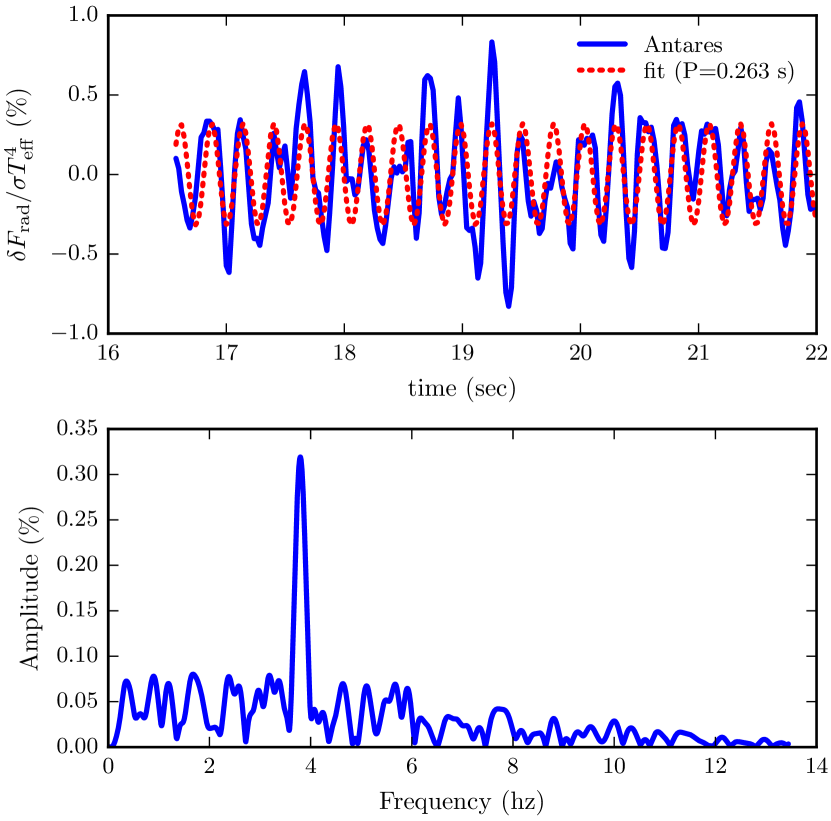
Figure 14: Pressure oscillation mode in our numerical simulation, whose period is close to the sound crossing time. In the upper panel we show the fractional variation of the radiative flux emerging at the top of the simulation domain after division by a polynomial fit to remove the trend due to thermal relaxation (blue, solid curve); the dotted (red) curve shows the sinusoidal fit to these data. The lower panel gives the Fourier transform of the normalized flux variations, which indicates a mode with a period of 0.263 s and an amplitude of $\sim 0.3$%.

We also observe a stable oscillation, a vertical, global pressure mode without interior node, which is easily visible for the horizontally averaged, vertical mean velocity. It has a frequency of $\nu_{\rm osc}=3.7959\,{\rm Hz}$ and thus a period of $P_{\rm osc}=0.26344\,{\rm s}$. Its amplitude is $\sim 30~{}{\rm m\,s}^{-1}$ at $\sim 5.85$ km where $w_{\rm rms}\sim 105~{}{\rm m\,s}^{-1}$. It can also be identified in the emerging radiative flux even though in this case it is subject to perturbations by local events (shock fronts, etc.) and drift due to thermal relaxation (discussed in the context of Fig. 5). After removing the latter from $F_{\rm rad}(x=0\,{\rm km},t)$ by a polynomial fit, it is easy to extract the dominant mode frequency, as is demonstrated in Fig. 14. Once excited, this oscillation cannot be removed from the simulation by artificial damping, if that were attempted (we have done a number of experiments with 2D simulations to corroborate that), so evidently the convection zone in the simulation is able to feed the mode energetically at a sufficiently high rate against damping mechanisms (due to radiative losses, viscosity, etc.) to support this very stable amplitude. The mode is also present throughout the convection zone and even has its maximum amplitude right there where it provides just a small fraction of the kinetic energy of the flow.

The oscillation with a frequency of $\nu_{\rm osc}$ can also be identified when tracing hot or cold structures in Fig. 10h–i, in $w_{\rm rms}$, or in $F_{\rm rad}$ (see Fig. 5). Thus, the flow taking place in the region below 4 km is a combination of global waves and local, transient features. Its properties with respect to skewness, kurtosis, vorticity, the clear presence of a global vertical mode with a significant contribution ($\sim 10\%$) to the kinetic energy in that region, and the decrease of $\Phi$ (and thus the faster decrease of horizontal in comparison with vertical velocities) justifies its naming as wave–dominated region. But these properties are at variance with efficient mixing and we thus expect the mixing processes in the two regions, the overshooting zone proper and the wave–dominated region, to differ physically and in their efficiency.

Now one might use the velocity field found in the numerical simulation, as has been done before (Freytag et al. 1996, Tremblay et al. 2015, e.g.), and derive a depth below which diffusion velocities dominate and in this sense define an extent of the mixed region. We have to point out here a major caveat of this procedure: just as simulations of solar surface convection, which have open lower vertical boundaries, the solid, slip boundaries used for simulations with a radiative region at the bottom also reflect vertical waves. Thus, while fluid can leave or enter the domain only in the former case, both types of boundary conditions conserve momentum inside the box and create a reflecting layer for vertical waves at the bottom of the simulation box. For both cases waves in a real star should have smaller maximum amplitudes due to the simple fact that the mode mass contained in the simulation box is much smaller. Amplitudes of p-mode oscillations hence have to be scaled by mode mass (Stein & Nordlund, 2001) to be compared to observations (or models of the entire star). Although the theoretical explanation of waves excited in the overshooting zone proposed by Freytag et al. (1996) is based on ${\rm g}^{-}$-modes rather than p-modes, we expect the former also to be altered (towards exhibiting a much lower equilibrium amplitude) due to the fact that in a real star such waves connect to a much larger mass. Hence, we expect that the velocities obtained for the wave–dominated region are systematically overestimated compared to a model of a full star. A determination of the mixed region by means of $w_{\rm rms}$ then leads to an even more pronounced overestimation. Consequently, as an upper limit of the mixed region one should rather use $u_{\rm rms}$ and $v_{\rm rms}$ or an exponential fit of $\Phi$.

Having the inevitable overestimations by this procedure in mind and without a suitable method of scaling of the velocity fields yet at hands, we may also consider the linear fit of $\Phi$ which at least provides a lower estimate for mixing due to the processes in the wave–dominated region, if the velocities of the numerical simulation in that part are taken at face value. Indeed, if we extrapolate the linear fit of $\Phi$, it would reach a value of 1 at $\sim 7.67$ km, some 5.67 km below the lower boundary of where $\nabla>\nabla_{\rm ad}$ still holds. This hopefully provides a safe, lower limit for the extent of the well mixed region; it corresponds to a mass of $\log(1-M_{r}/M_{\star})\sim-12.7$ in our stellar model.

4.3.3 Mixing and accretion

For the case of steady-state accretion of metals, the observed surface abundance results from a competition between the accretion rate onto the surface and the settling rate of the metals at the base of the mixed region. Using the published values of Koester (2009, Tables 1 and 4), we can estimate the effect that mixing beneath the formally convective region has on the settling rates for trace amounts of metals in a hydrogen atmosphere white dwarf. If we assume that mixing only occurs in the region defined by the Schwarzschild criterion, the base of the mixed region would be at $\log(1-M_{r}/M_{\star})\sim-15.2$; interpolating in Tables 1 and 4 of Koester yields a settling time for carbon of $\tau_{-15.2}\sim 0.14\,$yr. On the other hand, if we assume the base of the mixed region is at $\log(1-M_{r}/M_{\star})\sim-13.9$, corresponding to the depth of penetration of the plumes, then we find the settling time of carbon is $\tau_{-13.9}\sim 1.4\,$yr. Finally, if we take the base of the mixed region to be $\log(1-M_{r}/M_{\star})\sim-12.7$ (where $\Phi=1$ is extrapolated from the ANTARES simulation), then we obtain a settling time for carbon of $\tau_{-12.7}\sim 12\,$yr. The ratio of this settling time to that assuming mixing only in the Schwarzschild unstable region is $\sim 87$. For the elements Na, Mg, Si, Ca, and Fe, we find similar ratios for the enhancement of their settling times, in the range of 50–97. Thus, including the mixing in the overshooting region has a very large effect on the computed settling times of metals in WD envelopes.

In a similar vein, we would like to examine the effect that a larger mixed region has on the inferred accretion rates, assuming steady-state accretion. From Eq. 6 of Koester (2009), $X_{\rm CZ}=\tau_{\rm CZ}\dot{M}_{X}(M_{\rm CZ})^{-1}$, where $X_{\rm CZ}$ is the mass fraction of element $X$ in the convection zone, $\tau_{\rm CZ}$ is the settling time at the base of the mixed region, $\dot{M}_{X}$ is the mass accretion rate of element $X$, and $M_{\rm CZ}$ is the mass of the mixed region. If we assume that $X_{\rm CZ}$ is fixed by the observations, then $\dot{M}_{X}\propto M_{\rm CZ}/\tau_{\rm CZ}$. Using $\log(1-M_{r}/M_{\star})\sim-15.2$ and $-13.9$ for the extent of the mixed region with and without overshooting, respectively, we find that including the overshooting region enhances the inferred accretion rates by factors of 1.6–2.5 for the set of metals previously considered. If instead we take the depth of the overshooting region to be at $\log(1-M_{r}/M_{\star})\sim-12.7$, then we find that the inferred accretion rates are enhanced by factors 3.2–6.3 for the same set of metals with respect to the no-overshooting case.

We point out here that the total mixed mass obtained from the linear fit of $\Phi$ with the requirement $\Phi\rightarrow 1$ is roughly 300 times larger than that contained in and above the Schwarzschild-unstable region. This number is similar to suggestions by Freytag et al. (1996), Koester (2009), and within the (much larger) range suggested by Tremblay et al. (2015).

5 Discussion and outlook

We have highlighted here that estimates for the extent of the mixed region underneath the surface convection zone of DA white dwarfs at intermediate effective temperatures ($T_{\rm eff}\approx 11\,800~{}{\rm K}$) as obtained from (3D) hydrodynamical simulations have to be revisited from a new perspective. This has become possible thanks to the larger (3D) simulation domain and the simulation being performed over a sufficient amount in time. The larger horizontal extent reduces artifacts by the periodic boundary conditions and allows a better sampling of statistical data due to a larger number of realizations. The larger vertical extent allows for the first time a clear identification of exponential decay of the velocity field, as a function of depth, underneath a region dominated by plumes. In the latter, exponential fits lack both accuracy, since the decay rate itself would have to be a function of depth, and also a physical basis, since the upper parts of the overshooting zone are completely dominated by plumes and their dynamics instead of waves (even though the latter are of course also present in that part of the simulation domain). In the plume–dominated region (once $F_{\rm conv}<0$) we find a linear decay with depth to provide a more accurate model and in this sense the simulations agree qualitatively and, roughly, quantitatively with solutions of Reynolds stress models for somewhat hotter objects (cf. Montgomery & Kupka 2004). The wave–dominated region, for which we confirm exponential decay of the vertical root mean square velocity, is not modelled by the Reynolds stress approach (as the time dependent mean velocity was assumed to be zero, so it cannot be included in the model used by Montgomery & Kupka 2004). Viewing our results at a more coarse level we also confirm some basic findings of earlier studies (especially from Freytag et al. 1996 and Tremblay et al. 2011, 2013, 2015) performed with different simulation codes and with smaller domain sizes.

Contrary to earlier work we stress here that the horizontal velocities, which decay more rapidly than the vertical ones in the wave–dominated region, provide an indication for a less efficient mixing. We also point out that the amplitudes due to waves obtained from this class of simulations should be expected to be systematically too large. Thus, while the convective mixing due to overshooting up to and including the plume–dominated region is on safe ground, its extension into the wave–dominated region is much less certain and certainly subject to gross overestimation. We thus provide a linear extrapolation based on horizontal velocities which might be used as a more conservative estimate of the extent of the convectively mixed region.

We emphasise here that our results have been obtained for the case of a DA white dwarf with a large amount of convective flux inside the unstable zone which features strong, long-lived plumes penetrating into the stably-stratified region. Further studies should clarify the dependencies of these results on $T_{\rm eff}$ and $\log(g)$, and, with respect to the wave-dominated region, on simulation depth and time.

Finally, we show that the extent of the mixed region can have a large effect on the computed settling times and accretion rates of metals in WDs also when using our more conservative estimates of the extent of mixing due to overshooting. While we think there is merit in the prescription we have adopted for defining the extent of the mixing region, it is probably a lower limit compared to results which assume mixing velocities to decrease exponentially with depth. More precise estimates of this kind clearly require further work, not only from the viewpoint of simulations, but also with respect to some theoretical aspects such as mixing efficiency of the encountered types of flows and characterizations of the effect of limited simulation domain sizes.

References

- Arcoragi & Fontaine (1980) Arcoragi J. P., Fontaine G., 1980, ApJ, 242, 1208
- Böhm & Cassinelli (1971) Böhm K. H., Cassinelli J., 1971, A&A, 12, 21
- Canuto & Dubovikov (1997) Canuto V. M., Dubovikov M., 1997, Astrophys. Jour., 484, L161
- Canuto & Dubovikov (1998) Canuto V. M., Dubovikov M., 1998, Astrophys. Jour., 493, 834
- Dupuis et al. (1992) Dupuis J., Fontaine G., Pelletier C., Wesemael F., 1992, ApJS, 82, 505
- Fontaine & van Horn (1976) Fontaine G., van Horn H. M., 1976, ApJS, 31, 467
- Freytag et al. (1996) Freytag B., Ludwig H.-G., Steffen M., 1996, Astron. Astrophys., 313, 497
- Gianninas et al. (2014) Gianninas A., Dufour P., Kilic M., Brown W. R., Bergeron P., Hermes J. J., 2014, ApJ, 794, 35
- Grimm-Strele et al. (2015a) Grimm-Strele H., Kupka F., Löw-Baselli B., Mundprecht E., Zaussinger F., Schiansky P., 2015a, New Astron., 34, 278
- Grimm-Strele et al. (2015b) Grimm-Strele H., Kupka F., Muthsam H., 2015b, Comp. Phys. Comm., 188, 7
- Happenhofer et al. (2013) Happenhofer N., Grimm-Strele H., F. K., Löw-Baselli B., Muthsam B., 2013, Journal of Computational Physics, 236, 96
- Herwig (2000) Herwig F., 2000, Astron. Astrophys., 360, 952
- Iglesias & Rogers (1996) Iglesias C., Rogers F., 1996, Astrophys. Jour., 464, 943
- Kippenhahn & Weigert (1994) Kippenhahn R., Weigert A., 1994, Stellar Structure and Evolution, 3rd corr. edn. Astronomy and Astrophysics Library, Springer, Berlin; New York
- Koester (2009) Koester D., 2009, A&A, 498, 517
- Koester & Wilken (2006) Koester D., Wilken D., 2006, A&A, 453, 1051
- Kupka (2009) Kupka F., 2009, Mem. della Soc. Astron. Ital., 80, 701
- Kupka & Muthsam (2017) Kupka F., Muthsam H., 2017, Living Rev. in Comp. Astrophys., 3:1, 159 pp.
- Kupka & Robinson (2007) Kupka F., Robinson F. J., 2007, Mon. Not. R. Astron. Soc., 374, 305
- Kupka et al. (2009) Kupka F., Ballot J., Muthsam H. J., 2009, Communications in Asteroseismology, 160, 30
- Montgomery & Kupka (2004) Montgomery M. H., Kupka F., 2004, Mon. Not. Roy. Astron. Soc., 350, 267
- Mundprecht et al. (2013) Mundprecht E., Muthsam H. J., Kupka F., 2013, Monthly Notices of the Royal Astronomical Society, 435, 3191
- Muthsam et al. (2010) Muthsam H., Kupka F., Löw-Baselli B., Obertscheider C., Langer M., Lenz P., 2010, New Astron., 15, 460
- Paczyński (1969) Paczyński B., 1969, Acta Astron., 19, 1
- Paczyński (1970) Paczyński B., 1970, Acta Astron., 20, 47
- Pamyatnykh (1999) Pamyatnykh A. A., 1999, Acta Astronomica, 49, 119
- Rogers et al. (1996) Rogers F., Swenson F., Iglesias C., 1996, Astrophys. Jour., 456, 902
- Siedentopf (1933) Siedentopf H., 1933, Astron. Nachr., 247, 297
- Stein & Nordlund (2001) Stein R. F., Nordlund Å., 2001, ApJ, 546, 585
- Tremblay et al. (2011) Tremblay P.-E., Ludwig H.-G., Steffen M., Bergeron P., Freytag B., 2011, Astron. Astrophys., 531, L19 (5 pp.)
- Tremblay et al. (2013) Tremblay P.-E., Ludwig H.-G., Steffen M., Freytag B., 2013, Astron. Astrophys., 552, A13 (13 pp.)
- Tremblay et al. (2015) Tremblay P.-E., Ludwig H.-G., Freytag B., Fontaine G., Steffen M., Brassard P., 2015, Astrophys. Jour., 799, 142 (14 pp.)
- Zahn (1991) Zahn J.-P., 1991, Astron. Astrophys., 252, 179
- Zaussinger & Spruit (2013) Zaussinger F., Spruit H. C., 2013, Astron. Astrophys., 554, A119
- van Horn (1970) van Horn H. M., 1970, ApJ, 160, L53