A unified model for nucleosynthesis of heavy elements in stars

Abstract

We prospose a unified model for the nucleosynthesis of heavy ($A>57$) elements in stars. The neutron flux can be set to describe neutron capture in arbitrary neutron flux. Our approach solves the coupled differential equations, that describe the neutron capture and decays of 2696 nuclei, numerically without truncating those to include only either capture or decay as traditionally assumed in weak neutron flux ($s$ process). As a result the synthesis of heavy nuclei always evolves along a wide band in the valley of stable nuclei. The observed abundances in the Solar system are reproduced reasonably already in the simplest version of the model. The model predicts that the nucleosynthesis in weak or modest neutron flux produces elements that are traditionally assumed to result in the high neutron flux of supernovae explosions ($r$ process).

1 Introduction

The traditional approach for nucleosynthesis in stars that maintain weak neutron flux is the slow neutron capture process ($s$ process) that occurs along a path in the stability valley of nuclei. After the pioneering works of Burbidge et al. [1] and of Cameron [2], this process has been studied extensively in the literature [3]. The $s$-process approach starts with the coupled differential equations that describe the change (increase and decrease) of the abundance $N_{A}$ of a certain nucleus of atomic number $A$ at time $t$ due to neutron capture and the decrease of the abundance due to $\beta$ decay,

$$\frac{{\mathrm{d}}N_{A}}{{\mathrm{d}}t}(t)=N_{n}(t){\langle}\sigma v{\rangle}_{A-1}N_{A-1}(t)-N_{n}(t){\langle}\sigma v{\rangle}_{A}N_{A}(t)-\Gamma^{(\beta)}_{A}N_{A}(t)\,,$$ (1)

where $N_{n}(t)$ is the neutron density at time $t$, ${\langle}\sigma v{\rangle}_{A}$ is the neutron-capture reaction rate per neutron on a nucleus with mass number $A$ and $\Gamma^{(\beta)}=\ln 2/T^{(\beta)}_{1/2}$ denotes the $\beta$-decay width of the isotope ($T^{(\beta)}_{1/2}$ is the half life). For the large number of possible nuclei involved in this process, the standard way of finding an approximate solution is to assume that either the capture is much faster than the decay, or vice versa. With this assumption the nucleosynthesis of heavy elements evolves along a line in the valley of stable nuclei, called the $s$-process path.

The reaction rate depends on time through the variation of temperature. It is usually assumed that the temperature is constant during neutron irradiation, the typical value being $T=3.5\cdot 10^{8}$ K, corresponding to $kT=30$ keV. Then one may use ${\langle}\sigma v{\rangle}_{A}={\langle}\sigma_{T}{\rangle}_{A}v_{T}$ where ${\langle}\sigma_{T}{\rangle}_{A}$ is the Maxwellian-averaged cross section of neutron capture, that has the typical value of 100 mb, and $v_{T}=\sqrt{2kT/m_{n}}\simeq 2.4\cdot 10^{8}$ cm/s.

The classical $s$-process model can describe the observed abundances of $s$-process heavy elements surprisingly well provided one assumes two components of exponentially decaying neutron irradiation, the larger exposure main component and the smaller exposure weak component. A usual experimental confirmation of the $s$-process abundance is the comparison of the model prediction for the neutron capture cross section times abundance as a function of the mass number (see e.g. Fig. 19. in Ref. [3].) We note that this comparison involves only those nuclei which belong to the $s$-process path.

2 The model

While the classical $s$-process model gives a simple and fairly accurate description of the observed abundances of heavy elements, it certainly has some simplifying features that are worth a closer look. One point is that no matter how low the probability of a certain capture or decay process, if the sample of nuclei is sufficiently large, such events will occur in reality. This means that the evolution of nucleosynthesis along the $s$-process path can only be a simple approximation and one has to discuss carefully the conclusions drawn from the model. With present day computing capacity it is actually not necessary to make the simplifying assumptions that lead to the $s$-process path of evolution. Instead, we choose to solve the full system of differential equations numerically with some different kind of simplifying assumptions.

If we choose to keep all terms in Eq. (1), then we as well can include more terms that may have some relevance. If we do not force the evolution onto a path, then we can find increment of a given abundance $N_{A}$ by $\alpha$ decay from an already existing nucleus with two more proton and neutron number as well as decrement by possible $\alpha$ decay. This suggests that actually, the more correct abundance to follow is $N_{Z,N}(t)$, the abundance of the nuclei of a certain element with atomic number $Z$. Therefore, instead of Eq. (1), we choose to solve the coupled differential equations with one element as

$$\begin{split}\frac{{\mathrm{d}}N_{Z,N}}{{\mathrm{d}}t}&=N_{n}(t){\langle}\sigma v{\rangle}_{A-1}N_{Z,N-1}(t)+\Gamma^{(\beta)}_{Z-1,N+1}N_{Z-1,N+1}(t)+\Gamma^{(\alpha)}_{Z+2,N+2}N_{Z+2,N+2}(t)\\ &-N_{n}(t){\langle}\sigma v{\rangle}_{A}N_{Z,N}(t)-\Gamma^{(\beta)}_{Z,N}N_{Z,N}(t)-\Gamma^{(\alpha)}_{Z,N}N_{Z,N}(t)\,,\end{split}$$ (2)

where $\Gamma^{(\alpha)}=\ln 2/T^{(\alpha)}_{1/2}$ denotes the $\alpha$-decay width of the nuclei.This equation reflects the fact that the spectral analysis for observing a particular nucleus applies to fixed atomic numbers, not mass numbers.

In order to solve the coupled system of equations numerically, we introduce discrete time steps $\tau$. If the rate of a certain process is sufficiently large compared to the time step, then the differential equations can be linearized

$$N_{Z,N}(t+\tau)=N_{Z,N}(t)+p^{(n)}_{Z,N-1}N_{Z,N-1}(t)+p^{(\beta)}_{Z-1,N+1}N_{Z-1,N+1}(t)+p^{(\alpha)}_{Z+2,N+2}N_{Z+2,N+2}(t)$$

$$\qquad\qquad\qquad\qquad\qquad-p^{(n)}_{Z,N}N_{Z,N}(t)-p^{(\beta)}_{Z,N}N_{Z,N}(t)-p^{(\alpha)}_{Z,N}N_{Z,N}(t)\,,$$ (3)

where $p^{(x)}_{Z,N}=\tau\lambda^{(x)}_{Z,N}$, with $\lambda^{(x)}$ being the capture or decay rate for process $x$. This equation could be used only if the time step is (much) smaller than any of the capture or decay inverse rates, so that all probabilities $p^{(x)}_{Z,N}$ are (much) smaller than one. This condition would make the computer code uselessly slow because of the often very small decay life times. In order to be able to choose a sufficiently large time step, we perform the evolution in two steps, a neutron capture period followed by a decay period in an alternating manner.

Given a distribution of abundances at a given moment $t$, $N_{Z,N}(t)$, in the first step we allow only neutron capture with (possibly time dependent) probability $p^{(n)}_{Z,N}$, which increases each $N_{Z,N}(t)$ with $p^{(n)}_{Z,N-1}N_{Z,N-1}(t)$ and decreases them with $p^{(n)}_{Z,N}N_{Z,N}(t)$, so the net change in the capture period is

$$\Delta N_{Z,N}^{\rm capt.}=p^{(n)}_{Z,N-1}N_{Z,N-1}-p^{(n)}_{Z,N}N_{Z,N}\,,$$ (4)

and we update each value of the abundances accordingly.

In the next time step the nuclei present at the end of the previous capture period are allowed to decay only. This decay will be described by the usual exponential decay, and the number of decayed nuclei of a given isotope at the end of the decay period will be

$$\Delta N_{Z,N}^{\rm dec.}(t+\tau)=N_{Z,N}(t)[1-\exp(-\Gamma_{Z,N}\,\tau)]\,.$$ (5)

In Eq. (5) $\Gamma_{Z,N}$ is the total decay width of an unstable isotope with atomic number $Z$ and neutron number $N$, the sum of the partial widths for the various possible decays, $\Gamma_{Z,N}=\sum_{i}\Gamma_{Z,N}^{(i)}$. If the half life of the isotope is long as compared to the time step, we can use the approximation

$$\Delta N_{Z,N}^{\rm dec.}(t+\tau)\simeq N_{Z,N}(t)\,\Gamma_{Z,N}\,\tau\,,$$ (6)

and the combined effect of the two time steps (Eqs. (4) and (5)) is equivalent to Eq. (3). If however, $\Gamma_{Z,N}\tau$ is not small the expansion in Eq. (6) cannot be used. We use Eq. (6) if $\Gamma_{Z,N}\tau<-\ln 0.99$, while Eq. (5) if $-\ln 0.99<\Gamma_{Z,N}\tau<-\ln 0.01$ and $\Delta N_{Z,N}^{\rm dec.}(t+\tau)=N_{Z,N}(t)$ if $\Gamma_{Z,N}\,\tau>-\ln 0.01$ (i.e. all nuclei decay immediately). The total number of nuclei does not change, only redistributed in this step because the nuclei disappearing from a certain type will turn into other types of nuclei in proportion to the partial widths of the possible decay modes.

We took the relevant neutron capture cross sections for given $Z$ and $N$ from Ref. [5], the nuclear decay rates from Ref. [6] and in the region around bismuth we used the nuclear decay data from Ref. [7]. We included the relevant nuclear data of 2696 nuclei of which 178 are stable.

3 Predictions

The neutron-capture rate of a nucleus is proportional to its neutron-capture cross section $\lambda=\Phi{\langle}\sigma_{T}{\rangle}$, where $\Phi=N_{n}v_{T}$ is the neutron flux. Using the value of the neutron density typically assumed in the $s$ process (the case of weak neutron flux), $N_{n}=10^{8}\,{\rm n\,cm^{-3}}$ and average speed of neutrons, $v_{T}=2.4\cdot 10^{8}$cm s^-1, the flux is $\Phi=2.4\cdot 10^{-11}$mb^-2s^-1. The evolution band obtained with this parameter is shown on Fig. 2 after five cycles of 2.4 million steps with successively decreasing time steps $\tau_{i}=10^{5-i}$ s ($i=1,\dots,5$). Thus the total evoulution time is about 845 y. The smaller time steps, the wider band. Thus large time steps approximate the $s$ process. The evolution starts with $3\cdot 10^{45}$ ⁵⁶Fe nuclei and ends up producing 1090 nuclei. The evolution always progresses along a band and increasing the neutron flux, the band gets wider.

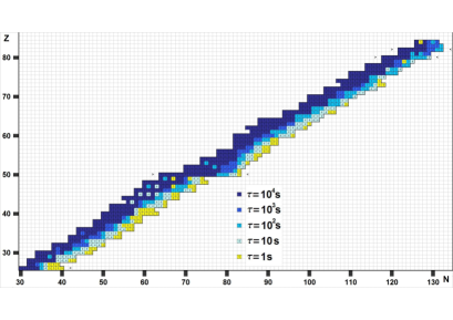
Figure 1: The evolution band obtained with $\Phi=2.4\cdot 10^{-11}$ mb^-2s^-1. The numbers in the boxes denote the cycle in which the given nucleus appeared.

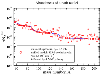
Figure 2: The abundances of elements obtained with $\Phi=2.4\cdot 10^{-8}$ mb^-2s^-1 in 845 y of evolution and 4.5 billion years of decay compared to the abundances obtained in the classical $s$ process.

Fig. 2 shows the predicted abundances of elements summed over isobars after two steps: (i) an initial evolution of 845 y with $\Phi=2.4\cdot 10^{-8}$ mb^-2s^-1 followed by (ii) a decay of 4.5 billion years. We compare our prediction to abundances resulting from the classical $s$ process (obtained with the same nuclear input). We see that our model gives identical results to the classical $s$ process.

The nucleosynthesis in our model evolves along a band in the stability valley until it seemingly stops at the $\alpha$-decaying isotopes of polonium, the $Z=84$ line. However, with existing neutron flux the number of heavy nuclei constantly increases. The decay process is probabilistic, therefore, not all nuclei decay in a given period. If the neutron flux is maintained for sufficiently long time, the band widens below the $Z=84$ line until it reaches ²¹⁸Bi. The time needed for the appearance of ²¹⁸Bi depends on the neutron flux. For instance, choosing $\Phi=2.4\cdot 10^{-8}$ mb^-2s^-1 (corresponding to $N_{n}=10^{11}\,{\rm n\,cm^{-3}}$), it takes about one year. The larger the flux, the shorter the required time. Once ²¹⁸Bi appears, heavier nuclei can easily be produced and appear quickly up to fermium (²⁶⁰Fm).

The rate of the evolution of trans-bismuth elements also correlates with the neutron flux: the larger $\Phi$, the faster evolution. After the neutron irradiance ceases, the unstable heavy nuclei decay quickly. However, some nuclei with long life time, such as ${}^{235}U$ and ${}^{238}U$, remain for a long time. The abundances of such nuclei depend strongly on the neutron density. For the relatively modest value of $N_{n}=10^{11}\,{\rm n\,cm^{-3}}$ the abundances of uranium isotopes is negligible as compared to the observable abundances of elements [8]. The observed abundances can be obtained with the model with the parameter value $\Phi\simeq 3\cdot 10^{-5}$ mb^-2s^-1 corresponding to $N_{n}\simeq 10^{14}\,{\rm n\,cm^{-3}}$ that is still six orders of magnitude smaller than the typical neutron density in supernovae [4].

Another interesting observation is that some elements, that do not belong to the $s$-process path (traditionally called $r$-only nuclei), also appear in the band with noticible abundances. This means that the band-like evolution reaches certain $r$-only nuclei even in the case of weak neutron flux, corresponding to $\Phi=2.4\cdot 10^{-11}$ mb^-2s^-1, although for such value the abundances of $r$-only nuclei are negligible. However, the observed abundances can be obtained with the still small value of $\Phi\simeq 10^{-9}$ mb^-2s^-1.

We proposed a model of nucleosythesis of heavy elements in stars. The main features of the model are the following: (i) all known neutron-capture and decay data of 2696 nuclei are taken into account, (ii) the coupled system of differential equations that describe the change of abundances of these nuclei is solved numerically. The model is very simple and does not take into account many effects that are considered standard in current analyses. Most importantly, the implementation of time-varying neutron flux is in progress.

This research was supported by the Hungarian Scientific Research Fund OTKA K-60432.

References

References

- [1] M. E. Burbidge, G. R. Burbidge, W. A. Fowler and F. Hoyle, “Synthesis of the elements in stars,” Rev. Mod. Phys. 29, 547 (1957).
- [2] A. G. W. Cameron, “Nuclear astrophysics,” Ann. Rev. Nucl. Part. Sci. 8, 299 (1958).
- [3] F. Käppeler, H. Beer and K. Wisshak “s-process nucleosynthesis – nuclear physics and the classical model,” Rep. Prog. Phys. 52, 945 (1989).
- [4] C.E. Rolfs and W.S. Rodney, “Cauldrons in the Cosmos,” The University of. Chicago Press, (1988).
- [5] http://physci.llnl.gov/Research/RRSN/semr/30kev.html, LLNL.
- [6] J. K. Tuli: Nuclear Wallet Cards 2005, BNL.
- [7] http://wwwndc.tokai-sc.jaea.go.jp; JENDL 3.3, Japan Atomic Energy Agency.
- [8] D. Arnett, “Supernovae and Nucleosynthesis”, Princeton Series in Astrophysics, (1996).