The magnitude of the minimal displacement vector
for compositions and convex combinations
of firmly nonexpansive mappings

Abstract

Maximally monotone operators and firmly nonexpansive mappings play key roles in modern optimization and nonlinear analysis. Five years ago, it was shown that if finitely many firmly nonexpansive operators are all asymptotically regular (i.e., the have or “almost have” fixed points), then the same is true for compositions and convex combinations.

In this paper, we derive bounds on the magnitude of the minimal displacement vectors of compositions and of convex combinations in terms of the displacement vectors of the underlying operators. Our results completely generalize earlier works. Moreover, we present various examples illustrating that our bounds are sharp.

2010 Mathematics Subject Classification: Primary 47H05, 47H09; Secondary 47H10, 90C25.

Keywords: Asymptotically regular, firmly nonexpansive mapping, maximally monotone operator, minimal displacement vector, nonexpansive mapping, resolvent.

1 Introduction and Standing Assumptions

Throughout this paper,

$$X \left\langle{\cdot},{\cdot}\right\rangle$$ is a real Hilbert space with inner product (1)

and induced norm $\|\cdot\|$. Recall that $T\colon X\to X$ is firmly nonexpansive (see, e.g., [3], [14], and [15] for further information) if $(\forall(x,y)\in X\times X)$ $\|Tx-Ty\|^{2}\leq\left\langle{x-y},{Tx-Ty}\right\rangle$ and that a set-valued operator $A\colon X\rightrightarrows X$ is maximally monotone if it is monotone, i.e., $\{(x,x^{*}),(y,y^{*})\}\subseteq\operatorname{gra}A\Rightarrow\left\langle{x-y},{x^{*}-y^{*}}\right\rangle\geq 0$ and if the graph of $A$ cannot be properly enlarged without destroying monotonicity. These notions are equivalent (see [18] and [12]) in the sense that if $A$ is maximally monotone, then its resolvent $J_{A}:=(\operatorname{Id}+A)^{-1}$ is firmly nonexpansive, and if $T$ is firmly nonexpansive, then $T^{-1}-\operatorname{Id}$ is maximally monotone.

In optimization, one main problem is to find zeros of (sums of) maximally monotone operators — these zeros may correspond to critical points or solutions to optimization problems. In terms of resolvents, the corresponding problem is that of finding fixed points. For background material in fixed point theory and monotone operator theory, we refer the reader to [3], [7], [8], [10], [14], [15], [21], [22], [24], [23], [25], [27], [28], and [26]. However, not every problem has a solution; equivalently, not every resolvent has a fixed point. To make this concrete, let us assume that $T\colon X\to X$ is firmly nonexpansive. The deviation from $T$ possessing a fixed point is captured by the notion of the minimal (negative) displacement vector which is well defined by

$$v_{T}:=P_{\overline{\operatorname{ran}}(\operatorname{Id}-T)}(0).$$ (2)

If $T$ “almost” has a fixed point in the sense that $v_{T}=0$, i.e., $0\in\overline{\operatorname{ran}}{(\operatorname{Id}-T)}$, then we say that $T$ is asymptotically regular. From now on, we assume that

$$I:=\{1,2,\ldots,m\} m\in\{2,3,4,\ldots\}$$, where

and that we are given $m$ firmly nonexpansive operators $T_{1},\ldots,T_{m}$; equivalently, $m$ resolvents of maximally monotone operators $A_{1},\ldots,A_{m}$:

$$(\forall i\in I)\quad T_{i}=J_{A_{i}}=(\operatorname{Id}+A_{i})^{-1}\;\;\text{is firmly nonexpansive,}$$

and we abbreviate the corresponding minimal displacement vectors by

$$(\forall i\in I)\quad v_{i}:=v_{T_{i}}=P_{\overline{\operatorname{ran}}(\operatorname{Id}-T_{i})}(0).$$ (3)

A natural question is the following: What can be said about the minimal displacement vector of $T$ when $T$ is either a composition or a convex combination of $T_{1},\ldots,T_{n}$?

Five years ago, the authors of [5] proved the following:

If each $T_{i}$ is asymptotically regular, then so are the corresponding compositions and convex combinations.

This can be expressed equivalently as

$$(\forall i\in I)\;\;v_{i}=0\quad\Rightarrow\quad v_{T}=0,$$ (4)

where $T$ is either a composition or a convex combination of the family $(T_{i})_{i\in I}$. It is noteworthy that these results have been studied recently by Kohlenbach [17] and [16] from the viewpoint of “proof mining”.

In this work, we obtain sharp bounds on the magnitude of the minimal displacement vector of $T$ that hold true without any assumption of asymptotic regularity of the given operators. The proofs rely on techniques that are new and that were introduced in [5] and [1] (where projectors were considered). The new results concerning compositions are presented in Section 2 while convex combinations are dealt with in Section 3. Finally, our notation is standard and follows [3] to which we also refer for standard facts not mentioned here.

2 Compositions

In this section, we explore compositions.

Proposition 2.1.

$(\forall\varepsilon>0)$ $(\exists x\in X)$ such that $\lVert x-T_{m}T_{m-1}\cdots T_{1}x\rVert\leq\varepsilon+\sum_{k=1}^{m}\lVert v_{k}\rVert$.

Proof. The proof is broken up into several steps. Set

$$(\forall i\in I)\quad\widetilde{A}_{i}:=-v_{i}+A_{i}(\cdot-v_{i}).$$ (5)

and observe that [3, Proposition 23.17(ii)&(iii)] yields

$$(\forall i\in I)\quad\widetilde{T}_{i}:=J_{\widetilde{A}_{i}}=v_{i}+J_{A_{i}}=v_{i}+T_{i}.$$ (6)

We also work in

$${\mathbf{X}}:=X^{m}=\big{\{}{\mathbf{x}=(x_{i})_{i\in I}}~{}\big{|}~{}{(\forall i\in I)\;x_{i}\in X}\big{\}},\quad\text{with}\;\;\left\langle{\mathbf{x}},{\mathbf{y}}\right\rangle=\sum_{i\in I}\left\langle{x_{i}},{y_{i}}\right\rangle,$$ (7)

where we embed the original operators via

$${\mathbf{T}}\colon X^{m}\to X^{m}\colon(x_{i})_{i\in I}\mapsto(T_{i}x_{i})_{i\in I}\;\;\text{and}\;\;{\mathbf{A}}\colon X^{m}\rightrightarrows X^{m}\colon(x_{i})_{i\in I}\mapsto\times(A_{i}x_{i})_{i\in I}.$$ (8)

Denoting the identity on $X^{m}$ by $\operatorname{\mathbf{Id}}$, we observe that

$$J_{{\mathbf{A}}}=(\operatorname{\mathbf{Id}}+{\mathbf{A}})^{-1}=T_{1}\times\cdots\times T_{m}={\mathbf{T}}.$$ (9)

Because ${\operatorname{ran}}(\operatorname{\mathbf{Id}}-{\mathbf{T}})=\operatorname{ran}(\operatorname{Id}-T_{1})\times\dots\times\operatorname{ran}(\operatorname{Id}-T_{m})$ and hence $\overline{\operatorname{ran}}(\operatorname{\mathbf{Id}}-{\mathbf{T}})=\overline{\operatorname{ran}}(\operatorname{Id}-T_{1})\times\dots\times\overline{\operatorname{ran}}(\operatorname{Id}-T_{m})$, we have (e.g., by using [3, Proposition 29.3])

$${\mathbf{v}}:=(v_{i})_{i\in I}=P_{\overline{\operatorname{ran}}(\operatorname{\mathbf{Id}}-{\mathbf{T}})}{\boldsymbol{0}}.$$ (10)

Finally, define the cyclic right-shift operator

$${\mathbf{R}}\colon X^{m}\to X^{m}\colon(x_{1},x_{2},\ldots,x_{m})\mapsto(x_{m},x_{1},\ldots,x_{m-1})\;\;\text{and}\;\;{\mathbf{M}}\coloneqq\operatorname{\mathbf{Id}}-{\mathbf{R}},$$ (11)

and the diagonal subspace

$${\boldsymbol{\Delta}}:=\big{\{}{\mathbf{x}=(x)_{i\in I}}~{}\big{|}~{}{x\in X}\big{\}},$$ (12)

with orthogonal complement ${\boldsymbol{\Delta}}^{\perp}$.

Claim 1: ${\mathbf{v}}\in\overline{\operatorname{ran}}\ ({\mathbf{A}}(\cdot-{\mathbf{v}})+{\mathbf{M}})$.
Indeed, 3 implies that $(\forall i\in I)$ $v_{i}\in\overline{\operatorname{ran}}\ (\operatorname{Id}-T_{i})=\overline{\operatorname{ran}}\ (\operatorname{Id}-J_{A_{i}})=\overline{\operatorname{ran}}\ J_{A_{i}^{-1}}=\overline{\operatorname{dom}}\ (\operatorname{Id}+A_{i}^{-1})=\overline{\operatorname{dom}}\ A_{i}^{-1}=\overline{\operatorname{ran}}\ A_{i}=\overline{\operatorname{ran}}\ A_{i}(\cdot-v_{i})$. Hence, ${\mathbf{v}}\in\overline{\operatorname{ran}}\ {\mathbf{A}}(\cdot-{\mathbf{v}})=\overline{\operatorname{ran}{\mathbf{A}}(\cdot-{\mathbf{v}})+{\boldsymbol{0}}}\subseteq\overline{\operatorname{ran}{\mathbf{A}}(\cdot-{\mathbf{v}})+{\boldsymbol{\Delta}}^{\perp}}$. On the other hand, we learn from [5, Corollary 2.6] (applied to ${\mathbf{A}}(\cdot-{\mathbf{v}})$) that $\overline{\operatorname{ran}}\ ({\mathbf{A}}(\cdot-{\mathbf{v}})+{\mathbf{M}})=\overline{\operatorname{ran}{\mathbf{A}}(\cdot-{\mathbf{v}})+{\boldsymbol{\Delta}}^{\perp}}$. Altogether, we obtain that ${\mathbf{v}}\in\overline{\operatorname{ran}}\ ({\mathbf{A}}(\cdot-{\mathbf{v}})+{\mathbf{M}})$ and Claim 1 is verified.

Claim 2: $(\forall\varepsilon>0)$ $(\exists(\mathbf{b},\mathbf{x})\in{\mathbf{X}}\times{\mathbf{X}})$ $\|\mathbf{b}\|\leq\varepsilon$ and $\mathbf{x}={\mathbf{v}}+{\mathbf{T}}(\mathbf{b}+{\mathbf{R}}\mathbf{x})$.
Fix $\varepsilon>0$. In view of Claim 1, there exists $\mathbf{x}\in{\mathbf{X}}$ and $\mathbf{b}\in{\mathbf{X}}$ such that $\|\mathbf{b}\|\leq\varepsilon$ and $\mathbf{b}\in-{\mathbf{v}}+{\mathbf{A}}(\mathbf{x}-{\mathbf{v}})+{\mathbf{M}}\mathbf{x}$. Hence, $\mathbf{b}+{\mathbf{R}}\mathbf{x}=\mathbf{b}+\mathbf{x}-{\mathbf{M}}\mathbf{x}\in\mathbf{x}+{\mathbf{A}}(\mathbf{x}-{\mathbf{v}})-{\mathbf{v}}=(\operatorname{\mathbf{Id}}+(-{\mathbf{v}}+{\mathbf{A}}(\cdot-{\mathbf{v}}))\mathbf{x}$. Thus, $\mathbf{x}=J_{-{\mathbf{v}}+{\mathbf{A}}(\cdot-{\mathbf{v}})}(\mathbf{b}+{\mathbf{R}}\mathbf{x})={\mathbf{v}}+{\mathbf{T}}(\mathbf{b}+{\mathbf{R}}\mathbf{x})$, where the last identity follows from 6, 9 and 10.

Claim 3: $(\forall\varepsilon>0)$ $(\exists(\mathbf{c},\mathbf{x})\in{\mathbf{X}}\times{\mathbf{X}})$ $\|\mathbf{c}\|\leq\varepsilon$ and $\mathbf{x}=\mathbf{c}+{\mathbf{v}}+{\mathbf{T}}({\mathbf{R}}\mathbf{x})$.
Fix $\varepsilon>0$, let $\mathbf{b}$ and $\mathbf{x}$ be as in Claim 2, and set $\mathbf{c}:=\mathbf{x}-{\mathbf{v}}-{\mathbf{T}}({\mathbf{R}}\mathbf{x})={\mathbf{T}}(\mathbf{b}+{\mathbf{R}}\mathbf{x})-{\mathbf{T}}({\mathbf{R}}\mathbf{x})$. Then, since ${\mathbf{T}}$ is nonexpansive, $\|\mathbf{c}\|=\|{\mathbf{T}}(\mathbf{b}+{\mathbf{R}}\mathbf{x})-{\mathbf{T}}({\mathbf{R}}\mathbf{x})\|\leq\|\mathbf{b}\|\leq\varepsilon$, and Claim 3 thus holds.

Conclusion:
Let $\varepsilon>0$. By Claim 3 (applied to $\varepsilon/\sqrt{m}$), there exists $(\mathbf{c},\mathbf{x})\in{\mathbf{X}}\times{\mathbf{X}}$ such that $\lVert\mathbf{c}\rVert\leq\varepsilon/\sqrt{m}$ and $\mathbf{x}=\mathbf{c}+{\mathbf{v}}+{\mathbf{T}}({\mathbf{R}}\mathbf{x})$. Hence $\sum_{i\in I}\|c_{i}\|\leq\|\mathbf{c}\|\sqrt{m}\leq\varepsilon$ and $(\forall i\in I)$ $x_{i}=c_{i}+v_{i}+T_{i}x_{i-1}$, where $x_{0}:=x_{m}$. The triangle inequality and the nonexpansiveness of each $T_{i}$ thus yields

$$\lVert T_{m}T_{m-1}\cdots T_{1}x_{0}-x_{0}\rVert =\lVert T_{m}T_{m-1}\cdots T_{1}x_{0}-x_{m}\rVert$$

$$=\big{\|}T_{m}T_{m-1}\cdots T_{2}T_{1}x_{0}-T_{m}T_{m-1}\cdots T_{2}x_{1}$$

$$\qquad+T_{m}T_{m-1}\cdots T_{3}T_{2}x_{1}-T_{m}T_{m-1}\cdots T_{3}x_{2}$$

$$\qquad+T_{m}T_{m-1}\cdots T_{4}T_{3}x_{2}-T_{m}T_{m-1}\cdots T_{4}x_{3}$$

$$\qquad+\cdots$$

$$\qquad+T_{m}T_{m-1}x_{m-2}-T_{m}x_{m-1}$$

$$\qquad+T_{m}x_{m-1}-x_{m}\big{\|}$$

$$\leq\lVert T_{m}T_{m-1}\cdots T_{2}T_{1}x_{0}-T_{m}T_{m-1}\cdots T_{2}x_{1}\rVert$$

$$\qquad+\lVert T_{m}T_{m-1}\cdots T_{3}T_{2}x_{1}-T_{m}T_{m-1}\cdots T_{3}x_{2}\rVert$$

$$\qquad+\lVert T_{m}T_{m-1}\cdots T_{4}T_{3}x_{2}-T_{m}T_{m-1}\cdots T_{4}x_{3}\rVert$$

$$\qquad+\cdots$$

$$\qquad+\lVert T_{m}T_{m-1}x_{m-2}-T_{m}x_{m-1}\rVert$$

$$\qquad+\lVert T_{m}x_{m-1}-x_{m}\rVert$$

$$\leq\lVert T_{1}x_{0}-x_{1}\rVert+\lVert T_{2}x_{1}-x_{2}\rVert+\lVert T_{3}x_{2}-x_{3}\rVert$$

$$\qquad+\cdots+\lVert T_{m-1}x_{m-2}-x_{m-1}\rVert+\lVert T_{m}x_{m-1}-x_{m}\rVert$$

$$=\lVert c_{1}+v_{1}\rVert+\lVert c_{2}+v_{2}\rVert+\cdots+\lVert c_{m}+v_{m}\rVert$$

$$\leq\sum_{k=1}^{m}\lVert c_{i}\rVert+\sum_{k=1}^{m}\lVert v_{i}\rVert$$

$$\leq\varepsilon+\sum_{k=1}^{m}\lVert v_{i}\rVert,$$ (13)

as claimed. $\hfill\quad\blacksquare$

We are now ready for our first main result.

Theorem 2.2.

$\displaystyle\lVert v_{T_{m}\cdots T_{2}T_{1}}\rVert\leq\lVert v_{T_{1}}\rVert+\cdots+\lVert v_{T_{m}}\rVert$.

Proof. By 2.1, we have $(\forall\varepsilon>0)$ $\lVert v_{T_{m}\cdots T_{2}T_{1}}\rVert\leq\varepsilon+\lVert v_{T_{1}}\rVert+\cdots+\lVert v_{T_{m}}\rVert$ and the result thus follows. $\hfill\quad\blacksquare$

As an immediate consequence of 2.2, we obtain the first main result of [5]:

Corollary 2.3.

[5, Corollary 3.2] Suppose that $v_{1}=\cdots=v_{m}=0$. Then $v_{T_{m}\cdots T_{2}T_{1}}=0$.

We now show that the bound on $\lVert v_{T_{m}\cdots T_{2}T_{1}}\rVert$ given in 2.2 is sharp:

Example 2.4.

Suppose that $X=\mathbb{R}$, $T_{1}\colon X\to X\colon x\mapsto x-a_{1}$, and $T_{2}\colon X\to X\colon x\mapsto x-a_{2}$, where $(a_{1},a_{2})\in\mathbb{R}\times\mathbb{R}$. Then $(v_{T_{1}},v_{T_{2}},v_{T_{2}T_{1}})=(a_{1},a_{2},a_{1}+a_{2})$ and $\lvert a_{1}+a_{2}\rvert=\lvert v_{T_{2}T_{1}}\rvert\leq\lvert v_{1}\rvert+\lvert v_{2}\rvert=\lvert a_{1}\rvert+\lvert a_{2}\rvert$; moreover, the inequality is an equality if and only if $a_{1}a_{2}\geq 0$.

Proof. On the one hand, it is clear that $\operatorname{ran}(\operatorname{Id}-T_{1})=\{a_{1}\}$ and likewise $\operatorname{ran}(\operatorname{Id}-T_{2})=\{a_{2}\}$. Consequently, $(v_{1},v_{2})=(a_{1},a_{2})$. On the other hand, $T_{2}T_{1}\colon X\to X\colon x\mapsto x-a_{1}-a_{2}=x-(a_{1}+a_{2})$, therefore $\operatorname{ran}(\operatorname{Id}-T_{2}T_{1})=\{a_{1}+a_{2}\}$. Hence, $v_{T_{2}T_{1}}=a_{1}+a_{2}$, $\lvert v_{T_{2}T_{1}}\rvert=\lvert a_{1}+a_{2}\rvert$ and $\lvert v_{1}\rvert+\lvert v_{2}\rvert=\lvert a_{1}\rvert+\lvert a_{2}\rvert$, and the conclusion follows. $\hfill\quad\blacksquare$

The remaining results in this section concern the effect of cyclically permuting the operators in the composition.

Proposition 2.5.

$v_{T_{m}T_{m-1}\cdots T_{2}T_{1}}=v_{T_{m-1}T_{m-2}\cdots T_{1}T_{m}}=\cdots=v_{T_{1}T_{m}\cdots T_{2}}$.

Proof. We start by proving that if $S_{1}\colon X\to X$ and $S_{2}\colon X\to X$ are averaged, then

$$v_{S_{2}S_{1}}=v_{S_{1}S_{2}}.$$ (14)

To this end, let $x\in X$ and note that $S_{2}S_{1}$ and $S_{1}S_{2}$ are $\alpha$-averaged where $\alpha\in[0,1[$ by, e.g., [3, Remark 4.34(iii) and Proposition 4.44]. Using [19, Proposition 2.5(ii)] applied to $S_{2}S_{1}$ and $S_{1}S_{2}$ yields

$$\lVert v_{S_{2}S_{1}}-v_{S_{1}S_{2}}\rVert^{2} \leftarrow\lVert(S_{2}S_{1})^{n}x-(S_{2}S_{1})^{n+1}x-((S_{1}S_{2})^{n}S_{1}x-(S_{1}S_{2})^{n+1}S_{1}x)\rVert^{2}$$

$$=\lVert(S_{2}S_{1})^{n}x-(S_{2}S_{1})^{n+1}x-(S_{1}(S_{2}S_{1})^{n}x-S_{1}(S_{2}S_{1})^{n+1}x)\rVert^{2}$$

$$=\lVert(\operatorname{Id}-S_{1})(S_{2}S_{1})^{n}x-(\operatorname{Id}-S_{1})(S_{2}S_{1})^{n+1}x\rVert^{2}$$

$$\leq\tfrac{\alpha}{1-\alpha}(\lVert(S_{2}S_{1})^{n}x-(S_{2}S_{1})^{n+1}x\rVert^{2}-\lVert S_{1}(S_{2}S_{1})^{n}x-S_{1}(S_{2}S_{1})^{n+1}x\rVert^{2})$$

$$\leq\tfrac{\alpha}{1-\alpha}(\lVert(S_{2}S_{1})^{n}x-(S_{2}S_{1})^{n+1}x\rVert^{2}-\lVert(S_{1}S_{2})^{n}S_{1}x-(S_{1}S_{2})^{n+1}S_{1}x\rVert^{2})$$

$$\to\tfrac{\alpha}{1-\alpha}(\lVert v_{S_{2}S_{1}}\rVert^{2}-\lVert v_{S_{1}S_{2}}\rVert^{2})=0,$$ (15)

where the last identity follows from [4, Lemma 2.6]. Because $T_{m-1}T_{m-2}\ldots T_{1}$ is averaged by [3, Remark 4.34(iii) and Proposition 4.44], we can and do apply 14, with $(S_{1},S_{2})$ replaced by $(T_{m-1}T_{m-2}\ldots T_{1},T_{m})$, to deduce that $v_{T_{m}T_{m-1}\cdots T_{2}T_{1}}=v_{T_{m-1}T_{m-2}\cdots T_{1}T_{m}}$. The remaining identities follow similarly. $\hfill\quad\blacksquare$

Proposition 2.6.

We have

$$v_{T_{m}T_{m-1}\cdots T_{1}}\in\operatorname{ran}(\operatorname{Id}-T_{m}T_{m-1}\cdots T_{1}) \Leftrightarrow v_{T_{m-1}\cdots T_{1}T_{m}}\in\operatorname{ran}(\operatorname{Id}-T_{m-1}\cdots T_{1}T_{m})$$ (16a)

$$\Leftrightarrow\cdots$$ (16b)

$$\Leftrightarrow v_{T_{1}T_{m}\cdots T_{2}}\in\operatorname{ran}(\operatorname{Id}-T_{1}T_{m}\ldots T_{2}).$$ (16c)

Proof. We prove the implication “$\Rightarrow$” of 16a: Suppose that $(\exists y\in X)$ $v_{T_{m}T_{m-1}\cdots T_{1}}=y-T_{m}T_{m-1}\cdots T_{1}y$, i.e., $y\in\operatorname{Fix}(v_{T_{m}\cdots T_{1}}+T_{m}\cdots T_{1})$. By [6, Proposition 2.5(iv)], we have $v_{T_{m}T\cdots T_{1}}=(T_{m}\cdots T_{1})y-(T_{m}\cdots T_{1})^{2}y$. Using 2.5, we obtain

$$\lVert v_{T_{m-1}\cdots T_{1}T_{m}}\rVert =\lVert v_{T_{m}\cdots T_{2}T_{1}}\rVert=\lVert(T_{m}T_{m-1}\cdots T_{1})y-(T_{m}T_{m-1}\cdots T_{1})^{2}y\rVert$$

$$\leq\lVert T_{m-1}\cdots T_{1}y-(T_{m-1}\cdots T_{1}T_{m})T_{m-1}\cdots T_{1}y\rVert$$

$$\leq\lVert y-T_{m}T_{m-1}\cdots T_{1}y\rVert=\lVert v_{T_{m}T_{m-1}\cdots T_{1}}\rVert=\lVert v_{T_{m-1}\cdots T_{1}T_{m}}\rVert.$$ (17)

Consequently, $\lVert v_{T_{m-1}\cdots T_{1}T_{m}}\rVert=\lVert T_{m-1}\cdots T_{1}y-(T_{m-1}\cdots T_{1}T_{m})T_{m-1}\cdots T_{1}y\rVert$ and hence

$$v_{T_{m-1}\ldots T_{1}T_{m}}=T_{m-1}\cdots T_{1}y-(T_{m-1}\cdots T_{1}T_{m})T_{m-1}\ldots T_{1}y\in\operatorname{ran}(\operatorname{Id}-T_{m-1}\ldots T_{1}T_{m}).$$ (18)

The opposite implication and the remaining $m-2$ equivalences are proved similarly. $\hfill\quad\blacksquare$

The following example, taken from De Pierro’s [11, Section 3 on page 193], illustrates that the conclusion of 2.6 does not necessarily hold if the operators are permuted noncyclically.

Example 2.7.

Suppose that $X=\mathbb{R}^{2}$, $m=3$, $C_{1}=\mathbb{R}\times\{0\}$, $C_{2}=\mathbb{R}\times\{1\}$, $C_{3}=\big{\{}{(x,y)\in\mathbb{R}^{2}}~{}\big{|}~{}{y\geq 1/x>0}\big{\}}$, and $(T_{1},T_{2},T_{3})=(P_{C_{1}},P_{C_{2}},P_{C_{3}})$. Then, $v_{T_{3}T_{2}T_{1}}=v_{T_{3}T_{1}T_{2}}=0$, $v_{T_{3}T_{2}T_{1}}\in\operatorname{ran}(\operatorname{Id}-T_{3}T_{2}T_{1})$ but $v_{T_{3}T_{1}T_{2}}\not\in\operatorname{ran}(\operatorname{Id}-T_{3}T_{1}T_{2})$.

Proof. Note that $T_{2}T_{1}=P_{C_{2}}P_{C_{1}}=P_{C_{2}}=T_{2}$ and $T_{1}T_{2}=P_{C_{1}}P_{C_{2}}=P_{C_{1}}=T_{1}$. Consequently, $(T_{3}T_{2}T_{1},T_{3}T_{1}T_{2})=(P_{C_{3}}P_{C_{2}},P_{C_{3}}P_{C_{1}})$. The claim that $v_{T_{3}T_{2}T_{1}}=v_{T_{3}T_{1}T_{2}}=0$ follows from [1, Theorem 3.1], or 2.2 applied with $m=3$. This and [2, Lemma 2.2(i)] imply that $\operatorname{Fix}T_{3}T_{2}T_{1}=\operatorname{Fix}P_{C_{3}}P_{C_{2}}=C_{3}\cap C_{2}\neq\varnothing$, whereas $\operatorname{Fix}T_{3}T_{1}T_{2}=\operatorname{Fix}P_{C_{3}}P_{C_{1}}=C_{3}\cap C_{1}=\varnothing$. Hence, $v_{T_{3}T_{2}T_{1}}\in\operatorname{ran}(\operatorname{Id}-T_{3}T_{2}T_{1})$ but $v_{T_{3}T_{1}T_{2}}\not\in\operatorname{ran}(\operatorname{Id}-T_{3}T_{1}T_{2})$. $\hfill\quad\blacksquare$

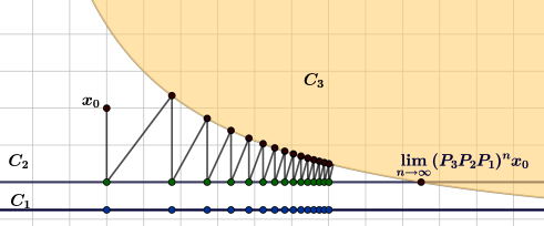
Figure 1: A GeoGebra [13] snapshot that illustrates the behaviour of the sequence $((P_{3}P_{2}P_{1})^{n}x_{0})_{n\in{\mathbb{N}}}$ in 2.6. The first few iterates of the sequences $(P_{1}(P_{3}P_{2}P_{1})^{n}x_{0})_{n\in{\mathbb{N}}}$ (blue points), $(P_{2}P_{1}(P_{3}P_{2}P_{1})^{n}x_{0})_{n\in{\mathbb{N}}}$ (green points), and $((P_{3}P_{2}P_{1})^{n}x_{0})_{n\in{\mathbb{N}}}$ (black points) are also depicted.

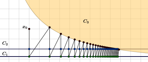
Figure 2: A GeoGebra [13] snapshot that illustrates the behaviour of the sequence $((P_{3}P_{1}P_{2})^{n}x_{0})_{n\in{\mathbb{N}}}$ in 2.6. The first few iterates of the sequences $(P_{1}(P_{3}P_{1}P_{2})^{n}x_{0})_{n\in{\mathbb{N}}}$ (green points), $(P_{2}P_{1}(P_{3}P_{1}P_{2})^{n}x_{0})_{n\in{\mathbb{N}}}$ (blue points), and $((P_{3}P_{1}P_{2})^{n}x_{0})_{n\in{\mathbb{N}}}$ (black points) are also depicted.

3 Convex Combinations

We start with the following useful lemma.

Lemma 3.1.

Suppose $(\forall i\in I)$ $A_{i}$ is $3^{*}$ monotone and $\operatorname{dom}A_{i}=X$. Let $(\alpha_{i})_{i\in I}$ be a family of nonnegative real numbers. Then the following hold:

1. $\sum_{i\in I}\alpha_{i}A_{i}$ is maximally monotone, $3^{*}$ monotone and $\operatorname{dom}\left(\sum_{i\in I}\alpha_{i}A_{i}\right)=X$.

2. $\overline{\operatorname{ran}}(\sum_{i\in I}\alpha_{i}A_{i})=\overline{\sum_{i\in I}\alpha_{i}\operatorname{ran}A_{i}}$.

Proof. Note that $(\forall i\in I)$, $\alpha_{i}A_{i}$ is maximally monotone, $3^{*}$ monotone and $\operatorname{dom}\alpha_{i}A_{i}=X$.

(i): The proof proceeds by induction. For $n=2$, the $3^{*}$ monotonicity of $\alpha_{1}A_{1}+\alpha_{2}A_{2}$ follows from [3, Proposition 25.22(ii)], whereas the maximal monotonicity of $\alpha_{1}A_{1}+\alpha_{2}A_{2}$ follows from, e.g., [3, Proposition 25.5(i)]. Now suppose that for some $n\geq 2$ it holds that $\sum_{i=1}^{n}\alpha_{i}A_{i}$ is maximally monotone and $3^{*}$ monotone. Then $\sum_{i=1}^{n+1}\alpha_{i}A_{i}=\sum_{i=1}^{n}\alpha_{i}A_{i}+\alpha_{n+1}A_{n+1}$, which is maximally monotone and $3^{*}$ monotone, where the conclusion follows from applying the base case with $(\alpha_{1},\alpha_{2},A_{1},A_{2})$ replaced by $(1,\alpha_{n+1},\sum_{i=1}^{n}\alpha_{i}A_{i},A_{n+1})$.

(ii): Combine (i) and [20, Corollary 6]. $\hfill\quad\blacksquare$

From this point onwards, let $(\lambda_{i})_{i\in I}$ be in $\left]0,1\right]$ with $\sum_{i\in I}\lambda_{i}=1$, and set

$$\overline{T}:=\sum_{i\in I}\lambda_{i}T_{i}.$$ (19)

We are now ready for our second main result.

Theorem 3.2.

$\lVert v_{\overline{T}}\rVert\leq\lVert\sum_{i\in I}\lambda_{i}v_{T_{i}}\rVert$.

Proof. It follows from [3, Examples 20.7 and 25.20] that $(\forall i\in I)$ $\operatorname{Id}-T_{i}$ is maximally monotone, $3^{*}$ monotone and $\operatorname{dom}(\operatorname{Id}-T_{i})=X$. This and 3.1(ii) (applied with $(\alpha_{i},A_{i})$ replaced by $(\lambda_{i},\operatorname{Id}-T_{i})$ imply that

$$\overline{\operatorname{ran}}\left(\operatorname{Id}-\overline{T}\right)=\overline{\operatorname{ran}}\sum_{i\in I}\lambda_{i}(\operatorname{Id}-T_{i})=\overline{\sum_{i\in I}\lambda_{i}\operatorname{ran}(\operatorname{Id}-T_{i})}.$$ (20)

Now, on the one hand, it follows from the definition of $v_{\overline{T}}$ that

$$\left(\forall y\in\overline{\operatorname{ran}}\left(\operatorname{Id}-\overline{T}\right)\right)\qquad\lVert v_{\overline{T}}\rVert\leq\lVert y\rVert.$$ (21)

On the other hand, the definition of $v_{i}$ implies that $(\forall i\in I)$ $v_{i}\in\overline{\operatorname{ran}}(\operatorname{Id}-T_{i})$. Hence, $\lambda_{i}v_{i}\in\lambda_{i}\ \overline{\operatorname{ran}}(\operatorname{Id}-T_{i})$. Therefore, $\sum_{i\in I}\lambda_{i}v_{i}\in\sum_{i\in I}\lambda_{i}\ \overline{\operatorname{ran}}(\operatorname{Id}-T_{i})\subseteq\overline{\sum_{i\in I}\lambda_{i}\ \operatorname{ran}(\operatorname{Id}-T_{i})}=\overline{\operatorname{ran}}\left(\operatorname{Id}-\overline{T}\right)$, where the last identity follows from 20. Now apply 21 with $y$ replaced by $\sum_{i\in I}\lambda_{i}v_{i}$. $\hfill\quad\blacksquare$

As an easy consequence of 3.2, we obtain the second main result of [5]:

Corollary 3.3.

[5, Theorem 5.5] Suppose that $v_{1}=\cdots=v_{m}=0$. Then $v_{\overline{T}}=0$.

The bound we provided in 3.2 is sharp as we illustrate now:

Example 3.4.

Let $a\in X$ and suppose that $T\colon X\to X\colon x\mapsto x-a$. Then $v_{T}=a$ and therefore $\operatorname{Fix}T\neq\varnothing\Leftrightarrow a=0$. Set $(\forall i\in I)$ $T_{i}=T$. Then $\overline{T}=\sum_{i\in I}\lambda_{i}T_{i}=T$, $(\forall i\in I)$ $v_{i}=v_{\overline{T}}=a$. Consequently, $\lVert v_{\overline{T}}\rVert=\lVert a\rVert=\lVert\sum_{i\in I}\lambda_{i}a\rVert=\lVert\sum_{i\in I}\lambda_{i}v_{i}\rVert$.

Example 3.4 suggests that the identity $v_{\overline{T}}=\sum_{i\in I}\lambda_{i}v_{i}$ holds true; however, the following example provides a negative answer to this conjecture.

Example 3.5.

Suppose that $m=2$, that $T_{1}\colon X\to X\colon x\mapsto x-a_{1}$, and that $T_{2}\colon X\to X\colon x\mapsto\tfrac{1}{2}x-a_{2}$, where $(a_{1},a_{2})\in(X\smallsetminus\{0\})\times X$. Then $\operatorname{ran}(\operatorname{Id}-T_{1})=\{a_{1}\}$, $\operatorname{ran}(\operatorname{Id}-T_{2})=X$, $\operatorname{ran}(\operatorname{Id}-\overline{T})=X$, and $0=v_{\overline{T}}\neq\lambda_{1}v_{1}+\lambda_{2}v_{2}=\lambda_{1}a_{1}$.

Proof. On the one hand, one can easily verify that $(v_{1},v_{2})=(a_{1},0)$; hence, $\lambda_{1}v_{1}+\lambda_{2}v_{2}=\lambda_{1}a_{1}\neq 0$. On the other hand, $\overline{T}\colon X\to X\colon x\mapsto\tfrac{\lambda_{1}+1}{2}x-(\lambda_{1}a_{1}+\lambda_{2}a_{2})$. Hence, $\overline{T}$ is a Banach contraction, and therefore, $\operatorname{Fix}\overline{T}\neq\varnothing$. Consequently, $v_{\overline{T}}=0$. $\hfill\quad\blacksquare$

References

[1]
H.H. Bauschke,
The composition of finitely many projections
onto closed convex sets in Hilbert space is
asymptotically regular, Proceedings of the
American Mathematical Society 131(2003), 141–146.
[2]
H.H. Bauschke and J.M. Borwein,
Dykstra’s alternating projection algorithm
for two sets,
Journal of Approximation
Theory 79 (1994), 418–443.
[3]
H.H. Bauschke and P.L. Combettes,
Convex Analysis and Monotone
Operator Theory in Hilbert Spaces,
Second Edition,
Springer, 2017.
[4]
H.H. Bauschke, W.L. Hare, and W.M. Moursi, Generalized solutions
for the sum of two maximally monotone operators,
SIAM Journal on Control and Optimization 52 (2014), 1034–1047.
[5]
H.H. Bauschke, V. Martin-Marquez, S.M. Moffat, and X. Wang,
Compositions and convex combinations of asymptotically
regular firmly nonexpansive mappings are also asymptotically
regular,
Fixed Point Theory and Applications (2012), 2012:53.
[6]
H.H. Bauschke and W.M. Moursi,
The Douglas–Rachford algorithm for two
(not necessarily intersecting) affine subspace,
SIAM Journal in Optimization 26,
968–985,
2016.
[7]
J.M. Borwein and J.D. Vanderwerff,
Convex Functions,
Cambridge University Press, 2010.
[8]
H. Brezis,
Operateurs Maximaux Monotones et
Semi-Groupes de Contractions dans les Espaces de Hilbert,
North-Holland/Elsevier, 1973.
[9]
H. Brezis and A. Haraux,
Image d’une Somme d’opérateurs Monotones et Applications,
Israel Journal of Mathematics 23 (1976), 165–186.
[10]
R.S. Burachik and A.N. Iusem,
Set-Valued Mappings and Enlargements
of Monotone Operators,
Springer-Verlag, 2008.
[11]
A. De Pierro,
From parallel to sequential projection methods
and vice versa in convex feasibility: results and conjectures.
In: Inherently parallel algorithms in feasibility
and optimization and their applications (Haifa, 2000), 187–201,
Studies in Computational Mathematics, 8 (2001), North-Holland, Amsterdam.
[12]
J. Eckstein and D.P. Bertsekas,
On the Douglas–Rachford splitting method
and the proximal point algorithm for maximal monotone
operators,
Mathematical Programming 55 (1992), 293–318.
[17]
U. Kohlenbach,
G. López-Acedo
and A. Nicolae,
Quantitative asymptotic regularity results for the composition of
two mappings,
Optimization 66 (2017),
1291–1299.
[18]
G.J. Minty,
Monotone (nonlinear) operators in Hilbert spaces,
Duke Mathematical Journal 29 (1962), 341–346.
[19]
W.M. Moursi, The forward-backward algorithm and the normal problem,
Journal of
optimization Theory and Applications (2017).
doi:10.1007/s10957-017-1113-4
[20]
T. Pennanen, On the range of monotone composite mappings,
Journal of Nonlinear and Convex Analysis 2 (2001), 193–202.
[21]
R.T. Rockafellar,
Convex Analysis,
Princeton University Press, Princeton, 1970.