A Pliable Lasso

Abstract

We propose a generalization of the lasso that allows the model coefficients to vary as a function of a general set of modifying variables. These modifiers might be variables such as gender, age or time. The paradigm is quite general, with each lasso coefficient modified by a sparse linear function of the modifying variables $Z$. The model is estimated in a hierarchical fashion to control the degrees of freedom and avoid overfitting. The modifying variables may be observed, observed only in the training set, or unobserved overall. There are connections of our proposal to varying coefficient models and high-dimensional interaction models. We present a computationally efficient algorithm for its optimization, with exact screening rules to facilitate application to large numbers of predictors. The method is illustrated on a number of different simulated and real examples.

1 Introduction

In this paper we consider the usual supervised learning problem. Given predictors $x_{ij}$ and response values $y_{i}$ for $i=1,2,\ldots N$ and $j=1,2,\ldots p$, one popular method for this problem is the lasso. This approach solves the $\ell_{1}$-penalized regression

$${\rm minimize}\;\frac{1}{2}\sum_{i=1}^{N}(y_{i}-\beta_{0}-\sum_{j=1}^{p}x_{ij}\beta_{j})^{2}+\lambda\sum_{j=1}^{p}|\beta_{j}|.$$ (1)

This is equivalent to minimizing the sum of squares with constraint $\sum|\beta_{j}|\leq s$. The absolute value penalty in (1) induces sparsity in the solution for sufficiently large values of $\lambda$; that is, some or many of the components of the solution $\hat{\beta}$ are zero. The lasso and associated techniques like the elastic net (Zou & Hastie (2005)) are widely used. The R language package glmnet solves the lasso as stated (1) and in a broader class of problems (such as generalized linear models) very efficiently, using a coordinate descent procedure. Note that the objective function in (1) is convex, making the optimization problem tractable.

In this paper we extend the lasso, embedding it in a more general model. We suppose that in addition to our predictors and outcome, we have measurements of one or more “modifying variables” $z_{ik}$ for $i=1,2\ldots N$ and $k=1,2,\ldots K$. For example, such a modifying variable might be sex (male or female), and we allow for the possibility that some or all of the coefficients $\beta_{j}$ are different for males and females. Or $Z$ might be time and we wish to allow time-varying coefficients. Another possibility is to choose the modifying variables to be some of the predictors $x_{ij}$.

Let $y$ be the $N-$vector of outcomes, and let $X,Z$ be $N\times p$ and $N\times K$ matrices containing values of the predictor and modifying variables respectively. Let $X_{j}$ be the $j$th column of $X$ (an $N$-vector), and let $\bf 1$ be a column $N$-vector of ones. The pliable lasso model has the form

$$\hat{y} = \beta_{0}{\bf 1}+\Delta_{0}(Z)+\sum_{j=1}^{p}X_{j}\circ(\beta_{j}{\bf 1}+\Delta_{j}(Z))$$ (2)

$$= \beta_{0}{\bf 1}+\Delta_{0}(Z)+\sum_{j=1}^{p}(X_{j}\beta_{j}+X_{j}\circ\Delta_{j}(Z))$$ (3)

In the above, $(\circ)$ is component-wise multiplication. In the first form, the $N$-vectors $\Delta_{j}(Z)$ are seen to modify the coefficients $\beta_{j}$; the second form expresses this equivalently as an interaction. Note that if all of the $\Delta_{j}(Z)$ are zero, then (3) reduces to the usual lasso.

For statistical power and interpretability, we also add an (asymmetric) weak hierarchy constraint:

$${\Delta_{j}(Z)\;{\mathbf{can\;be\;nonzero\;only\;if}\;}\beta_{j}\;{\mathbf{is\;nonzero}}}.$$ (4)

There are various possibilities for the form of $\Delta_{j}(Z)$. One idea is to estimate each $\Delta_{j}(Z)$ using the predicted values from a regression tree fit to $Z$. This is attractive because regression trees are simple and flexible, and can easily handle variables of different types. However the resulting optimization problem is non-convex, making computations challenging. We discuss this approach briefly in Section 8.

In our main proposal we assume instead that $\Delta_{j}(Z)$ is a linear function $Z\theta_{j}$, with $\theta_{j}$ an unknown $K$-vector. In that case the pliable lasso model (3) can be written as

$$\hat{y} = \beta_{0}{\bf 1}+Z\theta_{0}+\sum_{j=1}^{p}X_{j}(\beta_{j}{\bf 1}+Z\theta_{j})$$ (5)

$$= \beta_{0}{\bf 1}+Z\theta_{0}+X\beta+\sum_{j=1}^{p}(X_{j}\circ Z)\theta_{j}$$ (6)

with $(X_{j}\circ Z)$ denoting the $N\times K$ matrix formed by multiplying each column of $Z$ componentwise by the column vector $X_{j}$. We use the following objective function for this problem

$$J(\beta_{0},\theta_{0},\beta,\Theta)=\frac{1}{2N}\sum(y_{i}-\hat{y}_{i})^{2}+(1-\alpha)\lambda\sum_{j=1}^{p}\Bigl{(}(||(\beta_{j},\theta_{j})||_{2}+||\theta_{j}||_{2}\Bigr{)}+\alpha\lambda\sum_{j,k}|\theta_{jk}|_{1}.$$ (7)

Here $\Theta$ is a $p\times K$ matrix of parameters with $j$th row $\theta_{j}$ and individual entries $\theta_{jk}$, The quantities $\lambda$ and $\gamma$ are adjustable tuning parameters. The first term in the penalty enforces the hierarchy constraint (4) while the second term gives sparsity to the individual components of $\theta_{j}$. The parameter $\alpha$ controls the relative weight on the two penalties. Like the usual lasso, for fixed $\alpha$, we obtain a path of solutions indexed by the tuning parameter $\lambda$. In fact, as $\alpha\rightarrow 1$ (but is not equal to 1), the $\hat{\theta}_{j}$ are shrunk to zero and the problem yields solutions approaching those of the usual lasso. Note that the parameters $\beta_{0}$ and $\theta_{0}$ are left unpenalized.

Before we give more details, let’s see an example. With $N=100,p=20$ and standard normal predictors, we generated data from the model

$$y=3x_{1}+2x_{2}+3x_{2}\cdot I(z=0)+x_{3}+3x_{3}\cdot I(z=1)+0.3\epsilon,$$ (8)

Here $z$ is a single Bernoulli random variable and $\epsilon\sim N(0,1)$. Figure 1 shows the path of solutions as we vary $\lambda$.

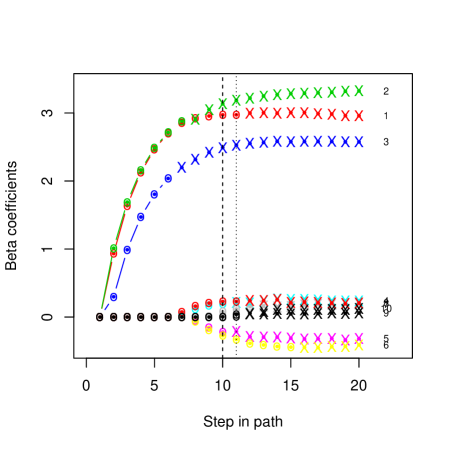
Figure 1: Solution path for Example 1. The “X” symbols indicates that the model has entered a modifying term $Z\theta_{j}$. The vertical dotted and broken lines show the model choice corresponding to minimum cross-validation and test error, respectively.

The vertical dotted and broken lines show the model choice corresponding to minimum cross-validation and test error, respectively. At these values, see that the model has correctly entered $X_{1}$ in the usual linear fashion and modifying terms for $X_{2}$ and $X_{3}$. It has also entered (incorrectly) small coefficients for some other predictors.

1.1 Related work

There are many connections between the proposal of this paper and previously published work. There is a close relationship to the class of varying coefficient models of Cleveland et al. (1991) and Hastie & Tibshirani (1993): the pliable lasso falls into this class, adding the notions of sparsity, hierarchy and scalability to the original proposals. Our proposed model is also a high-dimensional interaction model: recent work in this area includes Zhao et al. (2009), Bach et al. (2012), Bien et al. (2013), Lim & Hastie (2014), Pashova et al. (2016) , She et al. (2016), Haris et al. (2016) and Yan & Bien (2017). The use of the pliable lasso when $Z$ is unknown in the test set relates to the idea of customized training (Powers et al., 2015). This is discussed in the next section. The pliable lasso uses the penalties proposed in the group lasso (Yuan & Lin, 2007) and the sparse group lasso (Simon et al., 2013).

Unlike interaction models which treat variables all in the same manner, the pliable lasso is asymmetric in the way that the variables $X$ and $Z$ are treated. The $X$ variables are the main predictors in the model, and the modifying terms $\Theta_{jk}$ can only be nonzero if $\beta_{j}$ is non-zero. But the converse is not true. This is in contrast to other hierarchical interaction models for a set of predictors $X_{1},X_{2}\ldots X_{p}$: these use either weak hierarchy— the interaction between $X_{j}$ and $X_{k}$ is considered if at least one of their main effects is in the model—, or strong hierarchy, where both main effects have to be in the model. Examples are Bien et al. (2013) and Lim & Hastie (2014).

This latter procedure of Lim & Hastie (2014) (“Glinternet”) uses a latent overlapping group lasso whereas the pliable lasso uses a group lasso with overlapping groups. This distinction is made clear in Table 1 of Yan & Bien (2017). Glinternet models interactions between all pairs of variables, imposing strong hierarchy on the search: that is, an interaction can appear only if both main effects are in the model. Furthermore, the corresponding R package allows one to specify “interactionCandidates” : interactions are only considered between these variables and all other variables. To apply this procedure to our setting, we can take the set of variables to be $(X,Z)$ and then restrict interactions to the $Z$ variables. In this special case, this differs from the pliable lasso in the use of strong vs. weak hierarchy, and the fact that the pliable lasso interacts each $X_{j}$ with the entire vector $Z$. We compare Glinternet to the pliable lasso in the simulation examples in the next section.

1.2 Different use cases

An attractive property of the pliable lasso is its versatility. Table 1 summarizes the different possibilities.

Scenario	Training Set	Test Set	Examples
Known-Known	$Z$ known	$Z$ known	gender, age, $Z\subseteq X$
Known-Unknown	$Z$ known	$Z$ learned	time, patient ID
Unknown-Unknown	$Z$ learned	$Z$ learned	clusters from $X$

Table 1: Different possibilities for the modifying variables $Z$.

Scenario “Known-Known” is the simplest: we fit the pliable lasso model and apply it directly to the test set. One possibility is $Z\subseteq X$, that is, we take $Z$ equal to some (usually small) subset of the $X$ variables. This is illustrated in the HIV example Section 4. In Scenario “Known-Unknown”, we fit our model, but for prediction in the test set, we need to estimate the values of $z$ for the test set. For this purpose we apply a separate supervised learning procedure to predict $Z$ from $x$ in the training set, and then use the predicted values $\hat{Z}$ when applying the pliable lasso to the test set. This procedure may also use other information besides $X$, if available, to predict $Z$. In our example we use either a random forest or multinomial-lasso classifier.

In Scenario “Unknown-Unknown” we can form clusters based on $X$ (or any other available measurements) using either training data, or the combined training and test data. This scenario and also the scenario “Known-Unknown” when $Z$ is a categorical variable, relates closely to the customized training proposal of Powers et al. (2015). In that work, clusters are estimated from the training data, or the combined training and test sets, and then a local lasso model are fit to each of the clusters. In Section 7 we experiment with a different approach, estimating a linear contrast $Z=X\gamma$ from the data itself.

Here is an outline of the rest of this paper. Section 2 describes our optimization strategy, while Section 3 discusses a simulation study. Real data examples are explored in Section 4. Application of the pliable lasso to the estimation of heterogenous treatment effects is discussed in Section 5. Degrees of freedom of the fitted model is discussed in Section 6, while the setting of unknown $Z$ is covered in Section 7. Finally, we discuss extensions of the model in Section 8.

2 Optimization of the objective function.

The objective function (7) is convex, and for its minimization we use a blockwise cyclical coordinate descent procedure, over a path of decreasing $\lambda$ values using the previous solutions as warm starts. The problem has some attractive structure that simplifies the computation: in particular, fixing the other predictors, we have derived explicit conditions for determining if $(\hat{\beta}_{j},\hat{\theta}_{j})$ is nonzero and if it is nonzero, whether the $\hat{\theta}_{j}$ component is nonzero. If both are nonzero, we use a generalized gradient descent procedure to determine both parameters. This strategy makes for a fast algorithm, since we can cycle through the predictors and only do the costlier computation (generalized gradient descent) when needed.

The generic form of the algorithm is shown in Algorithm 1.

Algorithm 1 Algorithm for the Pliable Lasso

For a decreasing path of $\lambda$ values:

Repeat until convergence:

1. Compute $\hat{\beta}_{0}$ and $\hat{\theta}_{0}$ from the least squares regression of the current residual on $Z$.

2. For predictor $k=1,2,\ldots p,1,2,\ldots$

   (a) Check an (explicit) condition for $(\hat{\beta}_{j},\hat{\theta}_{j})=0$. if zero, skip to next $k$

   (b) Otherwise, compute $\hat{\beta}_{j}$ using soft-thresholding and then check the condition for $\hat{\theta}_{j}=0$. If zero, fix update $\hat{\beta}_{j}$ and then move to next $j$

   (c) Otherwise, if both ($\hat{\beta}_{j},\hat{\theta}_{j}$) are nonzero: use a generalized gradient procedure to find $(\hat{\beta}_{j},\hat{\theta}_{j})$.

The details of this procedure are given in the Appendix. As shown there, the condition used in Step 1 of the algorithm is

$$|X_{j}^{T}r_{(-j)}/N|\leq(1-\alpha)\lambda\;{\rm and}\;||S(W_{j}^{T}r_{(-j)}/N,\alpha\lambda)||_{2}\leq 2(1-\alpha)\lambda$$ (9)

where $r_{(-j)}$ is the partial residual with the fit for the $j$th predictor removed, $W_{j}=X_{j}\circ Z$ (elementwise multiplication in each column) and $S(x,t)={\rm sign}(x)(|x|-t)_{+}$ , the soft-threshold operator. We note the similarity to the standard coordinate descent procedure for the lasso (see e.g. Friedman et al. (2010)). Specifically, without the modifiers $Z$, the second condition disappears and the first expression is exactly the zeroness condition in the coordinate descent procedure for the lasso.

Remark A. We have included a factor $N$ in the denominator of the first term of the objective function in (7), to match the parameterization used in the glmnet program (Friedman et al., 2010) .

Remark B. The solutions to the optimization in (7) depend on the scaling to the $X$ and $Z$ variables. By default, we standardize each set to have zero mean and unit variance.

Remark C. In the coordinate descent procedure for the lasso procedure of Friedman et al. (2010)), using “naive” updates, the coefficient for each predictor can be checked and updated in $O(N)$ operations. In the current algorithm, this cost increases to $O(N\cdot K$) operations.

3 A simulation comparison

In this example we took $n=100,p=50$, and standard Gaussian independent predictors. The response was generated as

$$y = \mu(x)+0.5\cdot\epsilon;\;\;\epsilon\sim N(0,1)$$ (10)

$$\mu(x) = x_{1}\beta_{1}+x_{2}\beta_{2}+x_{3}(\beta_{3}e+2z_{1})+x_{4}\beta_{4}(e-2z_{2});\;\beta=(2,-2,2,2,0,\cdots)$$ (11)

with $e=(1,1,1\ldots 1)^{T}$. The modifying variables $Z$ were drawn from a simple Bernoulli distribution with equal probabilities. The signal to noise ratio was about 2. We applied the standard lasso, (using the R package glmnet), gradient boosting machines (using the R package gbm) , Glinternet (using the R package glinternet), and the pliable lasso over 20 simulations. The sample size $N$, $p$= number of $X$ variables, $K$=number of $Z$ variables are shown at the top of each panel.

Different variations of the problem are used in each panel, with details given in the figure caption. In every case the pliable lasso does best. As noted in the caption, all methods were run with default settings; while we didn’t tune the pliable lasso in any special way, it is possible that GBM and glinternet could perform better using different parameter settings. Of course GBM fits a much more general model than the pliable lasso and should perform better in more general settings, but it is reassuring than the pliable lasso does well across this range of problems.

Figure 2: Results from simulation experiment using model (11) and it variants. The methods are lasso, GBM, glinternet and the pliable lasso. The lasso, GBM and glinternet were given both $X$ and $Z$ as predictors. GBM used single split trees (stumps), which seems appropriate since the true interactions are first-order. In glinternet we only allowed interactions between $Z$ and the other predictors $X$. Otherwise, all methods were run with default settings and each used cross-validation to choose its tuning parameters. The top left panel uses model (11),with $N=100,p=10$, while top top right panels has $N=100,p=50$. In In the bottom left panel, we used $I(X_{j}>0)$ in place of each $X_{j}$, to give a potential advantage to GBM. In the bottom right we added strong main effect terms in $Z$, to aid the strong hierarchy strategy of glinternet.

4 Real data examples

4.1 A $Z\subseteq X$ example: HIV mutation data

Rhee et al. (2003) study six nucleotide reverse transcriptase inhibitors (NRTIs) that are used to treat HIV-1. The target of these drugs can become resistant through mutation, and they compare a collection of models for predicting these drug’s (log) susceptibility– a measure of drug resistance, based on the location of mutations. We focussed on the first drug (3TC), for which there are there are $p=217$ sites and $N=1057$ samples. We randomly divided the samples into approximately equal-sized training and test sets. In this case we chose the modifiying variables $Z$ to be a subset of the $X$ variables: we used the mutations having training set univariate $z$-scores $\geq 2$ in absolute value. Figure 3 shows the test error curves for the lasso and pliable lasso. We see that pliable lasso achieves somewhat lower test error than the lasso. The resulting model is easy to understand, involving some main effect mutations and some pairwise interactions between pairs of mutations.

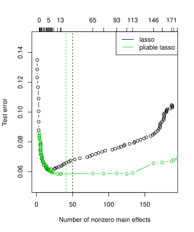
Figure 3: HIV mutation data: test error curves for the lasso and pliable lasso. The numbers across the top of the plot represent the number of main effects having interaction terms. The vertical broken lines show the choice of model from cross-validation.

4.2 Skin cancer proteomics data

The data in this example come from DESI mass spectometry measurements from tissues of patients with skin cancer, from collaborators here at Stanford. There are 16 patients in the training set, contributing with a total of 17,053 measurements (there are many image pixels per patient) and 2733 proteomic features. Each pixel is labelled as normal or cancer, with most patient samples consisting entirely of normal or cancer pixels. The test set had 7963 measurements from 9 patients. For computational ease we took a random sample of 1000 measurements from the training set and chose the 1000 features $X_{j}$ having largest univariate scores in the training set. We have used the lasso with success on similar data with other cancers, see e.g Eberlin et al. (2014).

Here we took $Z$ to be the patient ID. This is an example of the “known-unknown” scenario of Table 1: the patient IDs in the test set are different from those in the training set. Hence we fit a separate (multinomial-lasso) classifier in the training set, and use it to “predict” $Z$ in the test set. In other words, we find the training set patient most similar to a given test set patient, and use his/her patient ID for the prediction. To further enhance accuracy, we further filtered the $X_{j}$ variables, keeping the ones with univariate scores in the top 1000 for the outcome (as mentioned above ), but also required that they had scores in the top 1000 with respect to their variation between patients. This encourages the procedure to build a model on the training set that involves more predictable $Z$ variables, so that it will be more effective when applied to the test set. The second filtering left 437 features in the training set for the pliable lasso. The 16-class classifier for predicting patient ID in the training set had an cross-validation error rate of about 40%.

The resulting test set AUCs for the lasso and pliable lasso are shown in Figure 4. While the improvement shown by the pliable lasso over the lasso might seem small, it is actually quite significant: from a best rate of 94% for the lasso to about 97% for the pliable lasso.

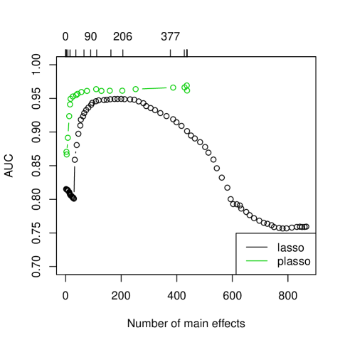
Figure 4: Skin cancer data: test set area under the curve for the lasso and pliable lasso, for various model sizes.

4.3 Forecasting example- predicting stock returns

Here is a another example of the “known-unknown” scenario of Table 1. The data are 21 day returns for a stock. We make daily predictions by fitting a lasso using 33 available signals as features. The training and test sets cover the periods 1997-2001 and 2002-2005 respectively. The base model uses a common lasso model fit to all of the training data. For the pliable lasso, we divided the training period into 10 equal time periods, and set $Z$ equal to the resulting ten category variable. We then built a random forest classifier to predict the most similar training period for each test date. Figure 5 depicts the classification of each test date.

Figure 5: Stock return data: each time on the right is classified as being most similar to the training time period indicated on the left.

The correlations of each predicted return with the actual return in the test set are shown in Figure 6. The pliable lasso achieves an increase of nearly 2% over the lasso, which could be quite significant practically.

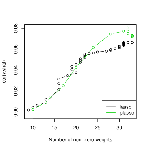
Figure 6: Stock return data: correlations between predicted and actual test period returns, for the lasso and pliable lasso.

4.4 Example: States crime data

In the section we analyze a public dataset on yearly state crime statistics, from 1977-2014, obtained from colleague John Donahue of Stanford law school. The outcome is violent crime rate and the predictors are 42 demographic variables. We created training and test sets by dividing the data into two approximately equal time periods. We first applied hierarchical clustering to the predictors, yielding the six regions depicted by Figure 7. We fit a pliable lasso model with $z$ equal to the six-category location. The test set error rates for the lasso and pliable lasso are shown in Figure 8. The choice of model size via cross-validation is indicated by the vertical broken lines in the plot. We used standard cross-validation, ignoring time ordering, and this produced a poor model size estimate for the lasso. Perhaps not surprisingly, the pliable lasso is able to use the region similarity to improved prediction. A heatmap of the modifying coefficients $\hat{\theta}_{jk}$ is shown in Figure 9. The unpenalized intercept $\hat{\theta}_{0}$ appears at the left and has the most effect. Two or three demographic predictors also vary across region. Note that the resulting model is somewhere in between a common model for all regions and separate linear model for each region.

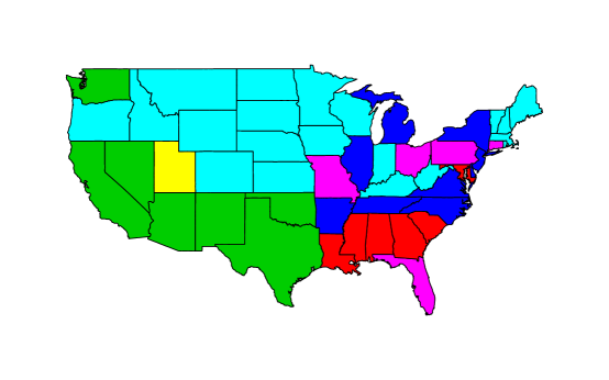
Figure 7: Crime data: grouping of states based on clustering of demographic variables.

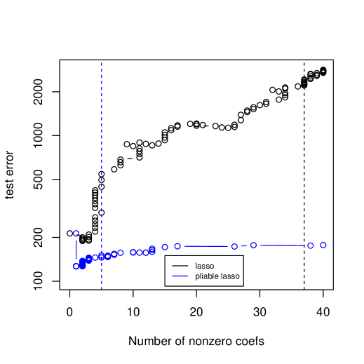
Figure 8: Test error rates for the crime data. The choice of model size via cross-validation is indicated by the vertical broken lines.

Figure 9: Crime data: estimated modifying coefficients $\hat{\theta}_{jk}$ for predictor $j$ (column of heatmap) and region $k$ (row of heatmap). Referring to colors of Figure 7, numbering is red=region 1, green=region 2, dark blue=region 3, light blue=region 4, purple=region 5, yellow=region 6.

5 Estimation of heterogenous treatment effects

The estimation of heterogenous treatment is a “hot” area of research, especially promising for the area of personalized medicine. The idea there is to find subsets of patients who will benefit from a specific treatment regime. This problem is especially challenging with high-dimensional features and observational data, that is, non-randomized treatment assignments. The small effect sizes seen in many real datasets makes the problem even more challenging. A review of recent work in this area is given by Powers et al. (2017). Here we briefly explore the application of the pliable lasso to this setting. Our data has the form $(X_{i},W_{i},Y_{i})$ where $X_{i}$ is a vector of covariates, $Y_{i}$ a real-valued response and $W_{i}\in\{0,1\}$ a treatment assignment. We assume that the treatment is randomly assigned with equal probability and make the usual unconfoundedness assumption. Extension to non-randomized studies via propensity scores is possible, but will not be explored here.

We use the pliable lasso model (6) with $Z=W$; the treatment effect at $x$ is estimated by $\hat{y}(x,W=1)-\hat{y}(x,W=1)$. With 50 standard normal predictors, we generated 100 observations from three different models:

$$(A):\;y = x_{1}+x_{1}w+x_{2}+2x_{3}+2\epsilon;\;\epsilon\sim N(0,1)$$ (12)

$$(B):\;y = x_{1}(w-0.5)+x_{2}+2x_{3}+2\epsilon;\;\epsilon\sim N(0,1)$$ (13)

$$(C):\;y = x_{1}+I(x_{1}>0)w+x_{2}+2x_{3}+2\epsilon;\;\epsilon\sim N(0,1)$$ (14)

The signal to noise ratio is about 1.5. Note that scenario A in the “home court” for the pliable lasso, with a single linear hierarchical interaction. Scenario B has a non-hierarchical interaction, centered with respect to the main effect. In Scenario C the interaction is hierarchical, but the predictor $X_{1}$ is dichotomized at 0.

We compared the pliable lasso approach to causal forests (Wager & Athey, 2015), a state of the art method for this problem. It is implemented in the generalized random forest package of Athey et al. (2016): we used version 0.9.3 with default settings. For scenarios A and B, the pliable lasso performs best: the advantage in (B) seems surprising— perhaps the random imbalance in treatment assignment creates a small main effect for $X$. In Scenario C, where the causal forest can split $x_{1}$ appropriately, it shows smaller variance than the pliable lasso, but with some bias. Of course the causal forest might perform better with other parameter settings, and is able to model much more general, high-order interactions than the pliable lasso.

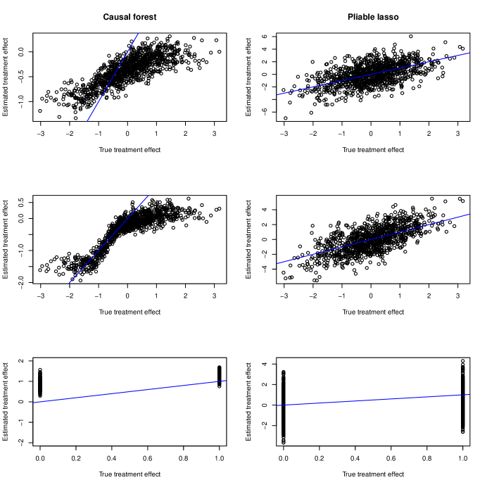
Figure 10: Results for causal forests and pliable lasso applied to the three problems in (14). The top, middle and bottom panels correspond to scenarios A, B, and C. The 45 degree line is drawn in blue each panel.

6 Degrees of freedom of the fit

Given a vector of response values $y$ and a fit vector $\hat{y}$, Efron (1986) defined the degrees of the fit by

$${\rm df}(\hat{y})\equiv\frac{\sum_{i}{\rm Cov}(y_{i},\hat{y}_{i})}{\sigma^{2}}$$ (15)

The power of this definition come from the fact that it can be applied to non-linear, adaptive estimators.

Now Efron et al. (2004) shows that if $y\sim N(\mu,I)$, then for the least angle regression procedure (a method for constructing the lasso path) after $k$ steps the degrees of freedom equals $k$. This result was strengthened and generalized in Zou et al. (2007) and Tibshirani & Taylor (2012) to show that for the lasso the number of non-zero elements in the solution is an unbiased estimated of the degrees of freedom.

Since the pliable lasso is a generalization of the lasso, we ask the question: how many degrees of freedom are spent in fitting a pliable lasso model with $k$ terms? In principle, this quantity may be analytically tractable but we have not yet succeeded in its derivation. Hence we turn to simulation to shed light on this question. In our setup, we take $N=100,p=5,10,20,50$, and generate standard normal predictors and the outcome from a null model and a non-null model with error variance one. The results are in Figure 11. We used estimated the covariance in (15) via the bootstrap, to provide an estimate of the degrees of freedom (horizontal axes).

Figure 11: Estimates of degrees of freedom for the pliable lasso, in the null setting (top panels) and the non-null setting (bottom panels). The degrees of freedom (horizontal axes) are estimated from the covariance formula, while the number of non-zero $\beta$ and $\theta$ parameters are shown in the left and right panels.

We see that the number of non-zero $\hat{\beta}_{j}$s provides a rough estimate of the degrees of freedom of the fit (left panels). On the other hand, the number of non-zero parameters including the $\hat{\theta}$s parameters is a gross over-estimate of the degrees of freedom (right panels). This is intuitively reasonable; the hierarchy constraint limits the number of modifying terms, when one does enter, the coefficients of both main effects and modifiers are shrunken. It would useful to investigate this rough “conjecture” in future work.

7 The setting of unknown $Z$

In this section we consider the pliable lasso model

$$\hat{y}=\beta_{0}{\bf 1}+Z\theta_{0}+X\beta+\sum_{j=1}^{p}(X_{j}\circ Z)\theta_{j}$$ (16)

but now assume that $Z$ is not observed. For simplicity we assume that $Z$ is a column vector that can be approximated by a linear function of $X$ that is $Z=X\gamma$, with $\gamma$ an unknown $p$-vector (extensions to matrix-valued $Z$ are also possible). We estimate $\gamma$ with an $\ell_{2}$ penalty. The objective function for the enlarged problem is

$$J(\beta_{0},\theta_{0},\beta,\Theta,\gamma)=\frac{1}{2n}\sum(y_{i}-\hat{y}_{i})^{2}+(1-\alpha)\lambda\sum_{j=1}^{p}\Bigl{(}(||(\beta_{j},\theta_{j})||_{2}+||\theta_{j}||_{2}\Bigr{)}+\alpha\lambda\sum_{j,k}|\theta_{jk}|_{1}+\frac{\lambda_{2}}{2}||\gamma||_{2}^{2}.$$ (17)

This problem is not convex, but is bi-convex— convex in $\gamma$ with other parameters fixed, and vice-versa.

The two subproblems can be easily solved. With $\hat{\gamma}$ fixed, we solve the original pliable lasso problem (7) with $Z=X\hat{\gamma}$. With the other parameters fixed, we write $W=\hat{\theta}_{0}X+\sum_{j=1}^{p}(X_{j}\hat{\theta}_{j}*X)$ and $r=y-\hat{\beta}_{0}-X\hat{\beta}$ and solve

$${\rm minimize}\frac{1}{2n}\sum(r_{i}-W\gamma)^{2}+\frac{\lambda_{2}}{2}||\gamma||_{2}^{2}$$ (18)

This is just a ridge regression without an intercept. In principal one could alternate these two steps until the procedure hopefully converges. I To investigate this procedure, we simulated data with $n=200,p=12$ in two regimes

$$y=x^{T}\beta_{z}+\sigma\epsilon;\;\;{\rm with}\;z=0:\beta_{0}=(2,2,2,2,0,\ldots 0);\;\;z=1:\beta_{1}=(-2,-2,-2,-2,0,\ldots 0);$$

Data were generated as $Pr(z=0|x)=1/(1+\exp(-x^{T}b_{z}))$ with $b=(0,0,\ldots 0,10,10,-10,10)$. The Bayes error for classifying $z$ from $x$ was 35%. We set $\sigma=0.25$ giving an SNR for $y$ of about 1.4. Figure 12 shows the result of applying just two cycles of the above procedure, starting with $\gamma$ equal to the least squares estimate of $y$ on $X$. The left panel shows the correlation between the estimated weights $\hat{\gamma}$ and the generating weights $b_{z}$. The right panel shows the test error for the pliable lasso (green) compared to the usual lasso (black). We see that in this idealized example, there is potential for learning the modifying variables from the data itself.

Figure 12: Results for pliable lasso, with modifying variables $Z$ unobserved. The left panel shows the correlation between the estimated weights $\hat{\gamma}$ and the generating weights $b_{z}$. The right panel shows the test error for the pliable lasso (green) compared to the usual lasso (black).

8 Further topics

(a) Tree-based pliable lasso. A more flexible version of the pliable lasso can be derived by using a regression tree to estimate the $\Delta_{j}(Z)$ factors in model 3. This allows for more general and higher order interactions between $X$ and $Z$. A coordinate descent algorithm can be derived for the resulting optimization, using a weighted regression tree fit. We have experimented with this idea with some success, but the non-convexity of the objective function makes it difficult to work with.

(b) Extensions to other models. The ideas presented here for the Gaussian regression model can be extended to other settings such as generalized linear models and the Cox proportional hazards model. One use can the standard Newton-style approach employed by the glmnet program, solving a weighted problem in the inner loop.

In the Cox model, $Z$ could be a set of modifying variables, as in the Gaussian model of this paper. But one could also use a categorical-valued $Z$ to denote the strata in a stratified Cox model. In more detail, the stratified Cox model assumes that the hazard function in the $k$th stratum has the form

$$h_{k}(t|x)=h_{0k}(t)e^{x^{T}\beta}$$ (19)

where $h_{0k}(t)$ is the baseline hazard function for the $k$th stratum. The log-partial likelihood is typically used for estimation, and is a sum over strata. We can generalize this model to

$$h_{k}(t|x)=h_{0k}(t)\exp[\sum_{j=1}^{p}x_{j}(\beta_{j}+\theta_{jk}I(Z=k))].$$ (20)

This would allow the effects of some features to vary over strata. In a similar way, one could choose $Z$ to index the risk sets in a survival analysis or the matched sets in a conditional logistic regression.

(c) Screening rules. A number of authors have proposed variable screening rules for speeding up the coordinate descent algorithm for the lasso and related procedures. These include El Ghaoui et al. (2010), Tibshirani et al. (2012), Wang et al. (2013) and Ndiaye et al. (2016). Since the objective function for the pliable lasso is closely related to the lasso and sparse group lasso, we are optimistic that effective screening rules could be derived for its optimization.

An R package for the pliable lasso will be made available in the CRAN library

Acknowledgements: We’d like to thank Jacob Bien and Leying Guan for helpful comments. Robert Tibshirani was supported by NIH grant 5R01 EB001988-16 and NSF grant 19 DMS1208164.

Appendix: details of the optimization

The pliable lasso model has the form

$$\hat{y}=\beta_{0}{\bf 1}+Z\theta_{0}+\sum_{j=1}^{p}(X_{j}\beta_{j}+W_{j}\theta_{j})$$

where $W_{j}=X_{j}\circ Z$ (elementwise multiplication in each column).

We note that $\beta_{0}$ and $\theta_{0}$ are optional components in the model, and are unpenalized when included. Hence for simplicity of notation we omit them from consideration: at the beginning of each pass over the predictors, we estimate $\beta_{0}$ and $\theta_{0}$ by regressing the current residual on $(1,Z$). In that case the outcome $y$ appearing below can be replaced by $y-\hat{\beta}_{0}-Z\hat{\theta}_{0}$.

The objective function is

$$J(\beta,\theta)=\frac{1}{2N}\sum(y_{i}-\hat{y}_{i})^{2}+(1-\alpha)\lambda\sum_{j=1}^{p}\Bigl{(}(||(\beta_{j},\theta_{j})||_{2}+||\theta_{j}||_{2}\Bigr{)}+\alpha\lambda\sum_{j,k}|\theta_{jk}|_{1}.$$

The subgradient equations are N

$$\frac{dJ}{d\beta_{j}} = -\frac{1}{N}X_{j}^{T}r+(1-\alpha)\lambda u=0$$ (21)

$$\frac{dJ}{d\theta_{j}} = -\frac{1}{N}W_{j}^{T}r+(1-\alpha)\lambda(u_{2}+u_{3})+\alpha\lambda v=0$$ (22)

where $r=y-\hat{y}$, and

$u=\frac{\beta_{j}}{||\beta_{j},\theta_{j}||_{2}}$ if $(\beta_{j},\theta_{j})\neq 0$ and $\in\{u:||u||_{2}\leq 1\}$ if $(\beta_{j},\theta_{j})=0$

$u_{2}=\frac{\theta_{j}}{||(\beta_{j},\theta_{j})||_{2}}$ if $(\beta_{j},\theta_{j})\neq 0$ and $\in\{u_{2}:||u_{2}||_{2}\leq 1\}$ if $(\beta_{j},\theta_{j})=0$

$u_{3}=\frac{\theta_{j}}{||\theta_{j}||_{2}}$ if $\theta_{j}\neq 0$ and $\in\{u_{3}:||u_{3}||_{2}\leq 1\}$ if $\theta_{j}=0$

$v\in{\rm sign}(\theta_{j})$

Screening conditions: Define the partial residual, leaving out the $j$th group, as

$$r_{(-j)}=y-\sum_{\ell\neq j}([X_{\ell}\hat{\beta}_{\ell}+W_{\ell}\hat{\theta}_{\ell}]$$

Then $(\hat{\beta}_{j},\hat{\theta}_{j})=0$ if

$$|X_{j}^{T}r_{(-j)}/N|\leq(1-\alpha)\lambda\;{\rm and}\;||S(W_{j}^{T}r_{(-j)}/N,\alpha\lambda)||_{2}\leq 2(1-\alpha)\lambda.$$ (23)

Otherwise we check if $\hat{\beta}_{j}\neq 0,\hat{\theta}_{j}=0$ by first computing

$$\hat{\beta}_{j}=(n/||X_{j}||_{2}^{2})\cdot S(X_{j}^{T}r_{-(j)}/N,(1-\alpha)\lambda)$$ (24)

and then checking if

$$||S(W_{j}^{T}(r_{(-j)}-X_{j}\hat{\beta}_{j})/N,\alpha\lambda)||_{2}\leq(1-\alpha)\lambda.$$ (25)

Iterations: (if $(\hat{\beta}_{j},\hat{\theta}_{j})\neq 0$):

Let $\gamma_{j}=(\beta_{j},\theta_{j})$. The majorized objective function is

$$M(\gamma_{j})=\ell_{0}+(\gamma_{j}-\gamma_{0})^{T}\nabla\ell+\frac{1}{2t}||\gamma_{j}-\gamma_{0}||_{2}^{2}+(1-\alpha)\lambda(||\gamma_{j}||_{2}+||\theta_{j}||_{2})+\alpha\lambda\sum_{j,k}|\theta_{jk}|_{1}$$

with $\ell_{0}=\nabla\ell(r_{(-j)},\gamma_{0})=(-X_{j}^{T}r_{(-j)}/N,-W_{j}^{T}r_{(-j)}/N$ for squared error loss.

This is equivalent to minimizing

$$\tilde{M}(\gamma_{j})=\frac{1}{2t}||\gamma_{j}-\gamma_{0}-t\nabla\ell)||_{2}^{2}+(1-\alpha)\lambda(||\gamma_{j}||_{2}+||\theta_{j}||_{2})+\alpha\lambda\sum_{j,k}|\theta_{jk}|_{1}.$$

Then $\hat{\beta}_{j},\hat{\gamma}$ satisfy

$$\Bigl{(}1+\frac{t(1-\alpha)\lambda}{||\hat{\gamma}_{j}||_{2}}\Bigr{)}\hat{\beta}_{j} = \beta_{0}-t\nabla_{\beta_{j}}\ell$$ (26)

$$\Bigl{(}1+t(1-\alpha)\lambda(\frac{1}{||\hat{\theta}_{j}||_{2}}+\frac{1}{||\hat{\gamma}_{j}||_{2}})\Bigr{)}\hat{\theta}_{j} = S(\theta_{0}-t\nabla_{\theta_{j}}\ell,t\alpha\lambda).$$ (27)

Let $a=||\hat{\beta}_{j}||_{2},b=||\hat{\theta}_{j}||_{2}$ so that $||\hat{\gamma}_{j}||_{2}=\sqrt{a^{2}+b^{2}}$. Take the norm of both sides in each equation above giving

$$\Bigl{(}1+\frac{t(1-\alpha)\lambda}{\sqrt{a^{2}+b^{2}}}\Bigr{)}a = |\beta_{0}-t\nabla_{\beta_{j}}\ell|$$ (28)

$$\Bigl{(}1+t(1-\alpha)\lambda(\frac{1}{b}+\frac{1}{\sqrt{a^{2}+b^{2}})})\Bigr{)}b = ||S(\theta_{0}-t\nabla_{\theta_{j}}\ell,t\alpha\lambda)||_{2}.$$ (29)

Defining $c=t(1-\alpha)\lambda$, $g_{1}=|\beta_{0}-t\nabla_{\beta_{j}}\ell|,g_{2}=||S(\theta_{0}-t\nabla_{\theta_{j}}\ell,t\alpha\lambda)||_{2}$, let $r_{1},r_{2}$ be the roots of the quadratic equation $r^{2}+2c_{1}r-2c_{1}g_{2}-g_{1}^{2}-g_{2}^{2}$. Then

$$\hat{a}=\frac{g_{1}u^{\prime}}{c+u^{\prime\prime}};\;\hat{b}=\frac{g_{1}v^{\prime}(c-g_{2})}{c+v^{\prime}}$$ (30)

where $u^{\prime},u^{\prime\prime},v^{\prime},v^{\prime\prime}$ are each equal to one of the roots $r_{1},r_{2}$ to satisfy (29).

Finally, the solutions $\hat{\beta}_{j},\hat{\theta}_{j}$ satisfy

$$\Bigl{(}1+\frac{t(1-\alpha)\lambda}{\sqrt{\hat{a}^{2}+\hat{b}^{2}}}\Bigr{)}\hat{\beta}_{j} = \beta_{0}-t\nabla_{\beta_{j}}\ell$$ (31)

$$\Bigl{(}1+t(1-\alpha)\lambda(\frac{1}{\hat{b}}+\frac{1}{\sqrt{\hat{a}^{2}+\hat{b}^{2}})})\Bigr{)}\hat{\theta}_{j} = S(\theta_{0}-t\nabla_{\theta_{j}}\ell,t\alpha\lambda)$$ (32)

Letting $c_{1},c_{2}$ be the constants multiplying $\hat{\beta}_{j}$ and $\hat{\theta}_{j}$ above, we have the update equations

$$\hat{\beta}_{j} = \frac{\beta_{0}-t\nabla_{\beta_{j}}\ell}{c_{1}}$$ (33)

$$\hat{\theta}_{j} = \frac{\||S(\theta_{0}-t\nabla_{\theta_{j}}\ell,t\alpha\lambda)||_{2}}{c_{2}}.$$ (34)

We use this to define updates $(\hat{\beta}_{j},\hat{\theta}_{j})\leftarrow U(\hat{\beta}_{j}^{old},\hat{\theta}_{j}^{old},t)$

All of this leads to the procedure given in Algorithm 1 below.

Algorithm 1 (Detailed) Algorithm for the Pliable Lasso

For a decreasing path of $\lambda$ values:

Repeat until convergence:

1. Compute $\hat{\beta}_{0}$ and $\hat{\theta}_{0}$ from the least squares regression of the current residual on $Z$.

2. For predictor $k=1,2,\ldots p,1,2,\ldots$

   (a) Check condition (23) for $(\hat{\beta}_{j},\hat{\theta}_{j})=0$. if zero, skip to next $k$

   (b) Otherwise, compute $\hat{\beta}_{j}$ from (24) and then check if $\hat{\theta}_{j}=0$ from (25). If zero, skip to next $k$

   (c) Otherwise, if both $\hat{\beta}_{j},\hat{\theta}_{j}$ are nonzero:

   Repeat until convergence

   (d) Solve equation (29) for the norms $a,b$ using (30)

   (e) Update $(\hat{\beta}_{j},\hat{\theta}_{j})\leftarrow U(\hat{\beta}_{j}^{old},\hat{\theta}_{j}^{old},t)$ from (34). (Nesterov acceleration and backtracking can be added for speed and to ensure convergence).

References

- (1)
- Athey et al. (2016) Athey, S., Tibshirani, J. & Wager, S. (2016), ‘Generalized Random Forests’, ArXiv e-prints .
-
Bach et al. (2012)
Bach, F., Jenatton, R., Mairal, J. & Obozinski, G. (2012), ‘Structured sparsity through convex optimization’,
Statist. Sci. 27(4), 450–468.
https://doi.org/10.1214/12-STS394 - Bien et al. (2013) Bien, J., Taylor, J. & Tibshirani, R. (2013), ‘A lasso for hierarchical interactions’, Annals of Statistics 42(3), 1111–1141.
- Cleveland et al. (1991) Cleveland, W., Grosse, E., Shyu, W. & Terpenning, I. (1991), Local regression models, in J. Chambers & T. Hastie, eds, ‘Statistical models in S’, Wadsworth.
- Eberlin et al. (2014) Eberlin, L. S., Tibshirani, R. J., Zhang, J., Longacre, T. A., Berry, G. J., Bingham, D. B., Norton, J. A., Zare, R. N. & Poultsides, G. A. (2014), ‘Molecular assessment of surgical-resection margins of gastric cancer by mass-spectrometric imaging’, Proceedings of the National Academy of Sciences 111(7), 2436–2441.
- Efron (1986) Efron, B. (1986), ‘How biased is the apparent error rate of a prediction rule?’, Journal of the American Statistical Association 81, 461–70.
- Efron et al. (2004) Efron, B., Hastie, T., Johnstone, I. & Tibshirani, R. (2004), ‘Least angle regression’, Annals of Statistics 32(2), 407–499. With discussion, and a rejoinder by the authors.
- El Ghaoui et al. (2010) El Ghaoui, L., Viallon, V. & Rabbani, T. (2010), ‘Safe feature elimination in sparse supervised learning’, Pacific journal of optimization 6(4), 667–698.
- Friedman et al. (2010) Friedman, J., Hastie, T. & Tibshirani, R. (2010), ‘Regularization paths for generalized linear models via coordinate descent’, Journal of Statistical Software 33, 1–22.
-
Haris et al. (2016)
Haris, A., Witten, D. & Simon, N. (2016), ‘Convex modeling of interactions with strong
heredity’, Journal of Computational and Graphical Statistics 25(4), 981–1004.
https://doi.org/10.1080/10618600.2015.1067217 - Hastie & Tibshirani (1993) Hastie, T. & Tibshirani, R. (1993), ‘Varying coefficient models (with discussion)’, J. Royal. Statist. Soc. B. 55, 757–796.
- Lim & Hastie (2014) Lim, M. & Hastie, T. (2014), ‘Learning interactions via hierarchical group-lasso regularization’, Journal of Computational and Graphical Statistics pp. 1–41.
- Ndiaye et al. (2016) Ndiaye, E., Fercoq, O., Gramfort, A. & Salmon, J. (2016), ‘GAP Safe Screening Rules for Sparse-Group-Lasso’, ArXiv e-prints .
-
Pashova et al. (2016)
Pashova, H., LeBlanc, M. & Kooperberg, C. (2016), ‘Structured detection of interactions with the
directed lasso’, Statistics in Biosciences .
https://doi.org/10.1007/s12561-016-9184-6 - Powers et al. (2015) Powers, S., Hastie, T. & Tibshirani, R. (2015), ‘Customized training with an application to mass spectrometric imaging of cancer tissue’, Ann. Appl. Stat. 9(4), 1709–1725.
- Powers et al. (2017) Powers, S., Qian, J., Jung, K., Schuler, A., Shah, N. H., Hastie, T. & Tibshirani, R. (2017), ‘Some methods for heterogeneous treatment effect estimation in high-dimensions’, ArXiv e-prints .
- Rhee et al. (2003) Rhee, S.-Y., Gonzales, M. J., Kantor, R., Betts, B. J., Ravela, J. & Shafer, R. W. (2003), ‘Human immunodeficiency virus reverse transcriptase and pro- tease sequence database’, Nucleic Acids Research 31, 298–303.
-
She et al. (2016)
She, Y., Wang, Z. & Jiang, H. (2016), ‘Group regularized estimation under structural
hierarchy’, Journal of the American Statistical Association 0(ja), 0–0.
https://doi.org/10.1080/01621459.2016.1260470 - Simon et al. (2013) Simon, N., Friedman, J., Hastie, T. & Tibshirani, R. (2013), ‘A sparse-group Lasso’, Journal of Computational and Graphical Statistics 22(2), 231–245.
- Tibshirani et al. (2012) Tibshirani, R., Bien, J., Friedman, J. Hastie, T., Simon, N. Taylor, J. & Tibshirani, R. (2012), ‘Strong rules for discarding predictors in lasso-type problems’, J. Royal Statistical Society B. pp. 245–266.
- Tibshirani & Taylor (2012) Tibshirani, R. J. & Taylor, J. (2012), ‘Degrees of freedom in lasso problems’, Annals of Statistics 40(2), 1198–1232.
- Wager & Athey (2015) Wager, S. & Athey, S. (2015), ‘Estimation and Inference of Heterogeneous Treatment Effects using Random Forests’, ArXiv e-prints .
- Wang et al. (2013) Wang, J., Lin, B., Gong, P., Wonka, P. & Ye, J. (2013), Lasso screening rules via dual polytope projection, in ‘Advances in Neural Information Processing Systems (NIPS Conference Proceedings)’, pp. 1070–1078.
-
Yan & Bien (2017)
Yan, X. & Bien, J. (2017),
‘Hierarchical sparse modeling: A choice of two group lasso formulations’,
Statist. Sci. 32(4), 531–560.
https://doi.org/10.1214/17-STS622 - Yuan & Lin (2007) Yuan, M. & Lin, Y. (2007), ‘Model selection and estimation in regression with grouped variables’, Journal of the Royal Statistical Society, Series B 68(1), 49–67.
- Zhao et al. (2009) Zhao, P., Rocha, G. & Yu, B. (2009), ‘The composite absolute penalties family for grouped and hierarchical variable selection’, Ann. Statist p. 3468–3497.
- Zou & Hastie (2005) Zou, H. & Hastie, T. (2005), ‘Regularization and variable selection via the elastic net’, Journal of the Royal Statistical Society Series B. 67(2), 301–320.
- Zou et al. (2007) Zou, H., Hastie, T. & Tibshirani, R. (2007), ‘On the degrees of freedom of the lasso’, The Annals of Statistics 35(5), 2173–2192.