From real materials to model Hamiltonians with density matrix downfolding

Due to advances in computer hardware and new algorithms, it is now possible to perform highly accurate many-body simulations of realistic materials with all their intrinsic complications. The success of these simulations leaves us with a conundrum: how do we extract useful physical models and insight from these simulations? In this article, we present a formal theory of downfolding–extracting an effective Hamiltonian from first-principles calculations. The theory maps the downfolding problem into fitting information derived from wave functions sampled from a low-energy subspace of the full Hilbert space. Since this fitting process most commonly uses reduced density matrices, we term it density matrix downfolding (DMD).

I Introduction to downfolding the many electron problem

In multiscale modeling of many-particle systems, the effective Hamiltonian (or Lagrangian) is one of the most core concepts. The effective Hamiltonian dictates the behavior of the system on a coarse-grained level, where ‘sub-grid’ effects are folded into the parameters and form of the effective Hamiltonian. Many concepts in condensed matter physics can be viewed as statements about the behavior of the effective Hamiltonian. In particular, identification of ‘strongly correlated’ materials as materials where band theory is not an accurate representation of the systems is a statement about effective Hamiltonians. Effective Hamiltonians at different length scales also form the basis of the renormalization group Wilson . A major goal in condensed matter physics is to determine what effective Hamiltonians apply to different physical situations, in particular quantum effective Hamiltonians, which lead to large-scale emergent quantum phenomena.

The dominant effective model for quantum particles in condensed systems is band structure, and for metals, Fermi liquid theory. However, a major challenge is how this paradigm should be altered when it is no longer a good description of the physical system. Examples of these include the high-T_c cuprates and other transition metal oxides, which do not appear to be well-described by these simple effective Hamiltonians. For these systems, many models have been proposed, such as the Hubbard Hubbard1963 , Kanamori Kanamori1963 , $t$-$J$ tJSpalek and Heisenberg models. While these models have been extensively studied analytically and numerically, and have significantly enhanced our understanding of the physics of correlated electrons, their effectiveness for describing a real complex system of interest is often unclear. At the same time, more complex effective models can be commensurately more difficult to solve, so one would like to also find an accurate effective model that is computationally tractable.

To address the need for a link between ab initio electron-level models and larger scale models, downfolding has most commonly been carried out using approaches based on density functional theory (DFT). The one particle part is obtained from a standard DFT calculation which is projected onto localized Wannier functions and gives an estimate of the effective hoppings of the lattice model based on Kohn-Sham band structure calculations Pavirini . Then, to estimate the interactions, one assumes a model of screening of the Coulomb interactions based on constrained DFT, RPA, or some other methods. Since effects of interactions between the orbitals of interest have already been accounted for by DFT, a double counting correction is required to obtain the final downfolded Hamiltonian. The approach has been developed and widely applied Pavirini ; Dasgupta ; Aryasetiawan2004 ; Jeschke2013 ; but remains an active area of research Haule_doublecounting . There are other downfolding approaches that include the traditional Löwdin method, coupled to a stochastic approach Tenno ; Zhou_Ceperley and the related method of canonical transformations White_CT ; Yanai_CT . While they have many advantages, it is typically not possible to know if a given model ansatz was a good guess or not, and it is very rare for a technique to provide an estimate of the quality of the resultant model.

The situation described above stands in contrast to the derivation of effective classical models. For concreteness, let us discuss classical force fields computed from ab initio electronic structure calculations. Typically, a data set is generated using an ab initio calculation in which the positions of the atoms and molecules are varied, creating a set of positions and energies. The parameters in the force field ansatz are varied to obtain a best-fit classical model. Then, using standard statistical tools, it is possible to assess how well the fit reproduces the ab initio data within the calculation, without appealing to experiment. While translating that error to error in properties is not a trivial task, this approach has the important advantage that in the limit of a high quality fit and high quality ab initio results, the resultant model is predictive.

Naïvely, one might think to reconcile the fitting approach used in classical force fields with quantum models by matching eigenstates between a quantum model and ab initio systems, varying the model parameters until the eigenstates match Wagner2013 . However, this strategy does not work well in practice because it is often not possible to obtain exact eigenstates for either the model or the ab initio system. To resolve this, we develop a general theory for generating effective quantum models that is exact when the wave functions are sampled from the manifold of low-energy states. Because this method is based on fitting the energy functional, we will show the practical application of this theory using both exact solutions and ab initio quantum Monte Carlo (QMC) to derive several different quantum models.

The endeavor we pursue here is to develop a multi-scale approach in which the effective interactions between quasiparticles (such as dressed electrons) are determined after an ab initio simulation (but not necessarily exact solution) of the continuum Schroedinger equation involving all the electrons. The method uses reduced density matrices (RDMs), of low-energy states, not necessarily eigenstates, to cast downfolding as a fitting problem. We thus call it density matrix downfolding (DMD). In this paper, our application of DMD to physical problems employ one body (1-RDM) and two body (2-RDM) density matrices. The many-body states used in DMD will typically be generated using QMC techniques [either variational Monte Carlo (VMC) or diffusion Monte Carlo (DMC)] to come close to the low energy manifold.

The remainder of the paper is organized as follows:

• In Section II, we clarify and make precise what it means to downfold a many-electron problem to a few-electron problem. We recast the problem into minimization of a cost function that needs to be optimized to connect the many and few body problems. We further these notions both in terms of physical as well as information science descriptions, which allows us to connect to compression algorithms in the machine learning literature.

• Section III discusses several representative examples where we consider multiband lattice models and ab initio systems to downfold to a simpler lattice model.

• In Section IV, we discuss future prospects of applications of the DMD method, ongoing challenges and clear avenues for methodological improvements.

II Downfolding as a compression of the energy functional

II.1 Theory

Energy functional

Suppose we start with a quantum system with Hamiltonian $H$ and Hilbert space ${\mathcal{H}}$.

Definition 1.

Let the energy functional be $E[\Psi]=\frac{\bra{\Psi}H\ket{\Psi}}{\braket{\Psi}{\Psi}}$ for a wavefunction $\ket{\Psi}\in{\mathcal{H}}$.

Theorem 1.

$E[\Psi]$ has a critical point only where $\Psi$ is an eigenstate of $H$.

Proof.

$$\frac{\delta}{\delta\Psi^{*}}E[\Psi]=\frac{\delta}{\delta\Psi^{*}}\frac{\langle\Psi|H|\Psi\rangle}{\langle\Psi|\Psi\rangle}=\frac{H|\Psi\rangle}{\langle\Psi|\Psi\rangle}-\langle\Psi|H|\Psi\rangle\frac{|\Psi\rangle}{|\langle\Psi|\Psi\rangle|^{2}}=\frac{(H-E[\Psi])|\Psi\rangle}{\langle\Psi|\Psi\rangle}\,.$$ (1)

Therefore, $\frac{\delta}{\delta\Psi^{*}}E[\Psi]=0$ if and only if $(H-E[\Psi])|\Psi\rangle=0$, i.e., $\Psi$ is an eigenvector of $H$ corresponding to eigenvalue $E[\Psi]$. ∎

Low energy space

Definition 2.

Let $\mathcal{LE}(H,N)$ be a subset of ${\mathcal{H}}$ spanned by $N$ vectors given by the lowest energy solutions to $H\ket{\Psi_{i}}=E_{i}{\Psi_{i}}$.

Definition 3.

$H_{eff}$ is an operator on the Hilbert space ${\mathcal{LE}(H,N)}$.

Definition 4.

The effective model $E_{eff}[\Psi]=\frac{\bra{\Psi}H_{eff}\ket{\Psi}}{\braket{\Psi}{\Psi}}$ is a functional from $\mathcal{LE}\rightarrow\mathbb{R}$.

If $\ket{\Psi}\in\mathcal{LE}$ and $\ket{\Phi}\in{\mathcal{H}}\setminus\mathcal{LE}$, then $\ket{\Psi}\oplus\ket{\Phi}\in{\mathcal{H}}$. In the following, we will use the direct sum operator $\oplus 0$ to translate between the larger ${\mathcal{H}}$ and the smaller $\mathcal{LE}$.

Lemma 1.

Suppose that $\ket{\Psi}\in\mathcal{LE}$ and $\ket{\Phi}\in{\mathcal{H}}\setminus\mathcal{LE}$. Then $\left.\frac{\delta E[\Psi\oplus\Phi]}{\delta\Phi}\right|_{\Phi=0}=0$.

Proof.

$\langle\Psi\oplus 0|H|0\oplus\Phi\rangle=0$ because the two states have non-overlapping expansions in the eigenstates of $H$. Using that fact, we can evaluate

$$\left.\frac{\delta E[\Psi\oplus\Phi]}{\delta\Phi}\right|_{\Phi=0} =\left.\frac{\left(H-E[\Psi\oplus\Phi]\right)\ket{\Phi}}{\braket{\Psi}{\Psi}+\braket{\Phi}{\Phi}}\right|_{\Phi=0}=0.$$ (2)

∎

This is equivalent to noting that $H$ is block diagonal in the partitioning of ${\mathcal{H}}$ into $\mathcal{LE}$ and ${\mathcal{H}}\setminus\mathcal{LE}$. Importantly, if $\ket{\Psi}\in\mathcal{LE}$, then $\frac{\delta E[\Psi\oplus 0]}{\delta(\Psi\oplus 0)^{*}}=\ket{\Psi^{\prime}}\oplus 0$, where $\ket{\Psi^{\prime}}\in\mathcal{LE}$.

Theorem 2.

Assume $E[\Psi\oplus 0]=E_{eff}[\Psi]+C$ for any $\ket{\Psi}\in\mathcal{LE}$, where $C$ is a constant. Then $(H_{eff}+C)|\Psi\rangle\oplus 0=H(|\Psi\rangle\oplus 0)$.

Proof.

Note that

$$\frac{\delta E[\Psi\oplus 0]}{\delta(\Psi\oplus 0)^{*}}=\frac{(H-E[\Psi\oplus 0])\ket{\Psi\oplus 0}}{\braket{\Psi}{\Psi}}$$ (3)

and

$$\frac{\delta E_{eff}[\Psi]}{\delta\Psi^{*}}=\frac{(H_{eff}-E_{eff}[\Psi])\ket{\Psi}}{\braket{\Psi}{\Psi}}.$$ (4)

Since the derivatives are equal, setting Eq. (3) equal to Eq. (4),

$$H\ket{\Psi\oplus 0}=(H_{eff}+E[\Psi\oplus 0]-E_{eff}[\Psi])\ket{\Psi}\oplus 0=(H_{eff}+C)\ket{\Psi}\oplus 0.$$ (5)

∎

Theorem 2 combined with Lemma 1 means that the eigenstates of $H_{eff}$ are be the same as the eigenstates of $H$ if its derivatives match $H$. Such $H_{eff}$ always exists. Let $H_{eff}=\sum_{i}^{N}E_{i}|\Psi_{i}\rangle\langle\Psi_{i}|$ where $|\Psi_{i}\rangle$’s are eigenstates belong to $\mathcal{LE}(H,N)$. This satisfies $E[\Psi]=E_{eff}[\Psi]$ and $H_{eff}|\Psi\rangle=H|\Psi\rangle$ for any $\Psi$ in $\mathcal{LE}(H,N)$.

We have thus reduced the problem of finding an effective Hamiltonian $H_{eff}$ that reproduces the low-energy spectrum of $H$ to matching the corresponding energy functionals $E[\Psi]$ and $E_{eff}[\Psi]$. This involves sampling the low-energy space, choosing the form of $H_{eff}$, and optimizing the parameters. An important implication of this is that it is not necessary to diagonalize either of the Hamiltonians; one must only be able to select wave functions from the low-energy space $\mathcal{LE}$. As we shall see, this can be substantially easier than attaining eigenstates.

Some further notes about this derivation:

• Fitting $\Psi$’s must come from $\mathcal{LE}$. It is not enough that the energy functional $E[\Psi]$ is less than some cutoff.

• In the case of sampling an approximate $\mathcal{LE}$, the error comes from non-parallelity of $E[\Psi]$ with the correct low energy manifold, up to a constant offset.

• While $H_{eff}$ is unique, it has many potential representations and approximations.

• Our method can be applied to any manifold spanned by eigenstates

• Model fitting is finding a compact approximation to $E_{eff}[\Psi]$. This is a high-dimensional space, so we use descriptors to do this.

• For operators that are not the Hamiltonian, it is possible to fit $\mathcal{O}_{eff}[\Psi]\simeq{\mathcal{O}}[\Psi]$ in a similar way. However, the eigenstates of ${\mathcal{O}}$ and ${\mathcal{O}}_{eff}$ will not coincide in general unless $\mathcal{O}$ commutes with the Hamiltonian.

The theory presented above maps coarse-graining into a functional approximation problem. This is still rather intimidating, since even supposing one can generate wave functions in the low-energy space, they are still complicated objects in a very large space. An effective way to accomplish this is through the use of descriptors, $d_{i}[\Psi]$, which map from ${\mathcal{H}}\rightarrow\mathbb{R}$. Then we can approximate the energy functional as follows

$$E_{eff}[\Psi]\simeq\sum_{i}f_{i}(d_{i}[\Psi]),$$ (6)

where $f_{i}$ are some parameterized functions. This will allow us to use techniques from statistical learning to efficiently describe $E_{eff}$.

II.2 Practical protocol

Figure 1: A practical protocol for fitting effective models to ab initio data.

A practical protocol is presented in Figure 1. In this section we go through this procedure step by step.

Generating $\ket{\Psi_{i}}\in\mathcal{LE}$

Ideally one would be able to sample the entire low-energy space. Typically, however, the space will be too large and it will need to be sampled. The optimal wave functions to use depend on the models one expects to fit, which we will discuss in detail in later steps. Simple strategies that we will use in the examples below include excitations with respect to a determinant and varying spin states.

Generate $d_{j}[\Psi_{i}]$ and $E[\Psi_{i}]$

The choice of descriptor is fundamental to the success of the downfolding. In the case of a second-quantized Hamiltonian

$$H_{eff}=E_{0}+\sum_{ij}t_{ij}(c_{i}^{\dagger}c_{j}+h.c.)+\sum_{ijkl}V_{ijkl}c_{i}^{\dagger}c_{j}^{\dagger}c_{k}c_{l},$$ (7)

a set of linear descriptors by simply taking the expectation value of both sides of the equation. Then for example, the occupation descriptor for orbital $k$ is $d_{occ(k)}[\Psi_{i}]=\braket{\Psi_{i}}{c_{k}^{\dagger}c_{k}}{\Psi_{i}}$; the double occupation descriptor for orbital $k$ is $d_{double(k)}[\Psi_{i}]=\braket{\Psi_{i}}{n_{k\uparrow}n_{k\downarrow}}{\Psi_{i}}$. The orbital that $c_{k}$ represents is part of the descriptor, and in the examples below we will discuss this choice as well. One is not limited to static orbital descriptors; they may have a more complex functional dependence on the trial function to include orbital relaxation.

Assess descriptors

At this point, one has collected the data $E_{i}$ and $d_{ij}$. If two descriptors have a large correlation coefficient, then they are redundant in the data set. This could either mean that the sampling of the low-energy Hilbert space $\mathcal{LE}$ was insufficient, or that they are both proxies for the same differences in states. If two data points have the same or very similar descriptor sets, but different energies, then either the descriptor set is not enough to describe the variations in the low-energy space, or the sampling has generated states that are not in the low-energy space. To resolve these possibilities, one should analyze the difference between the two wave functions.

In either case, when the model is accurate, the fits will be accurate. If descriptors values available in the reduced Hilbert space are not represented in the sampled wave functions, then intruder states can appear upon solution of the effective model. In that case, the model fitting is an extrapolation instead of an interpolation. For this reason it is desirable to have eigenstates or near-eigenstates in the sample set if possible; they are guaranteed to be on the corners of the descriptor space if the model is accurate.

Ansatz: $E_{i}\simeq\sum_{i}d_{ij}p_{j}$

If the descriptors are chosen well, then the model can be written in linear form:

$$E[\Psi_{i}]=\sum_{j}p_{j}d_{j}[\Psi_{i}],$$ (8)

which we shorten to

$${\bf E}=D{\bf p}.$$ (9)

If this can be done, the fitting problem is reduced to a linear regression optimization. More complex functions of the descriptors are also possible, although at the cost of making the effective model more difficult to solve and complicating the fitting procedure.

Fit optimal model

Finally, one wishes to find a set of parameters such that Eq. (9) is satisfied as closely as possible. There are many choices to make in this step, which will often depend on the desired properties of the final model. One can imagine choosing different cost functions to minimize, which can also include a penalty for complicated models. In our tests, we have successfully used LASSO Lasso and matching pursuit techniques MP_Zhang1993 to select high quality and compact model parameters. A detailed example of using the latter technique is presented in Section III.4.

III Representative Examples

Given the theoretical framework for downfolding a many orbital (or many-electron) problem to a few orbital (or few-electron) problem, we now discuss examples which elucidate the DMD method. The examples are as follows:

• Section III.1: Three-band Hubbard $\rightarrow$ one-band Hubbard at half filling. Demonstrates finding a basis set for the second quantized operators and uses a set of eigenstates directly sampled from the low-energy space to find a one-band model.

• Section III.2: Hydrogen chain $\rightarrow$ one-band Hubbard model at half filling. Demonstrates basis sets for ab initio systems and the possibility to use this technique to determine the quality of a model to a given physical situation.

• Section III.3: Graphene $\rightarrow$ one-band Hubbard model with and without $\sigma$ electrons. Demonstrates using the downfolding procedure to examine the effects of screening due to core electrons.

• Section III.4: FeSe molecule $\rightarrow$ $3d,4p,4s$ system. Demonstrates the use of matching pursuit to assess the importance of terms in an effective model and to select compact effective models.

In all examples we will highlight the important ingredients associated with DMD. First and foremost is the choice of low energy space or energy window i.e. how our database of wave functions was generated. Associated with this is the choice of the one body space in terms of which the effective Hamiltonian is expressed. Finally, we discuss aspects of the functional forms or parameterizations that are expected to describe our physical problem. An important effective Hamiltonian that enters three out of our four representative examples is the one-band or single-band Hubbard model:

$$H=E_{0}-t\;\sum_{\langle i,j\rangle,\eta}\tilde{d}_{i,\eta}^{\dagger}\tilde{d}_{j,\eta}+U\;\sum_{i}\tilde{n}^{i}_{\uparrow}\tilde{n}^{i}_{\downarrow}\,,$$ (10)

where $t$ and $U$ are downfolded (renormalized) parameters, $\eta$ is a spin index, $\tilde{d}_{i,\eta}$ is the effective one-particle operator associated with spatial orbital (or site) $i$ and $n_{i,\eta}=\tilde{d}_{i,\eta}^{\dagger}\tilde{d}_{i,\eta}$ is the corresponding number operator. $\langle i,j\rangle$ is used to denote nearest neighbor pairs. We will sometimes drop the constant energy shift $E_{0}$ when we write equations like Eq. (10).

III.1 Three-band Hubbard model to one-band Hubbard model at half filling

Our first example is motivated by the high $T_{c}$ superconducting cuprates Bednorz1986 that have parent Mott insulators with rich phase diagrams on electron or hole doping Dagotto_RevModPhys ; LeeWen_RevModPhys . Many works have been devoted to their model Hamiltonians and corresponding parameter values tJSpalek ; Pavirini ; Emery ; ZhangRice ; Hybertsen_PRB1989 ; Hybertsen_PRB1990 ; Kent_Hubbard . A minimal model involving both the copper and oxygen degrees of freedom is the three-orbital or three-band Hubbard model,

$$H = \epsilon_{p}\sum_{j\in p,\eta}n_{j,\eta}+\epsilon_{d}\sum_{i\in d,\eta}n_{i,\eta}+t_{pd}\sum_{\langle i\in d,j\in p\rangle,\eta}\text{sgn}(p_{i},d_{j})\Big{(}c_{i,\eta}^{\dagger}c_{j,\eta}+\text{h.c.}\Big{)}$$ (11)

$$+U_{p}\sum_{j\in p}n_{j,\uparrow}n_{j,\downarrow}+U_{d}\sum_{i\in d}n_{i,\uparrow}n_{i,\downarrow}+V_{pd}\sum_{\langle i\in p,j\in d\rangle}n_{j}n_{i}\,,$$

where $d_{i},p_{j}$ refer to the $d_{x^{2}-y^{2}}$ orbitals of copper at site $i$ and $p_{x}$ or $p_{y}$ oxygen at site $j$, respectively. $\text{sgn}(p_{i},d_{j})$ is the sign of the hopping $t_{pd}$ between nearest neighbors, shown schematically in Figure 2. $\epsilon_{d}$ and $\epsilon_{p}$ are orbital energies, $U_{d}$ and $U_{p}$ are strengths of onsite Hubbard interactions, and $V_{pd}$ is the strength of the density-density interactions between a neighboring $p$ and $d$ orbital. To simplify we consider only the case where $\epsilon_{p}$, $U_{d}$ and $t_{pd}$ are non zero; $t_{pd}$ is chosen throughout this section to be the typical value of $1.3$ eV to give the reader a sense of overall energy scales. Since we work with fixed number of particles we set our reference zero energy to be $\epsilon_{d}=0$, thus the charge transfer energy $\Delta\equiv\epsilon_{p}-\epsilon_{d}$ equals $\epsilon_{p}$ in our notation. We work in the hole notation; half filling corresponds to two spin-up and two spin-down holes on the $2\times 2$ cell.

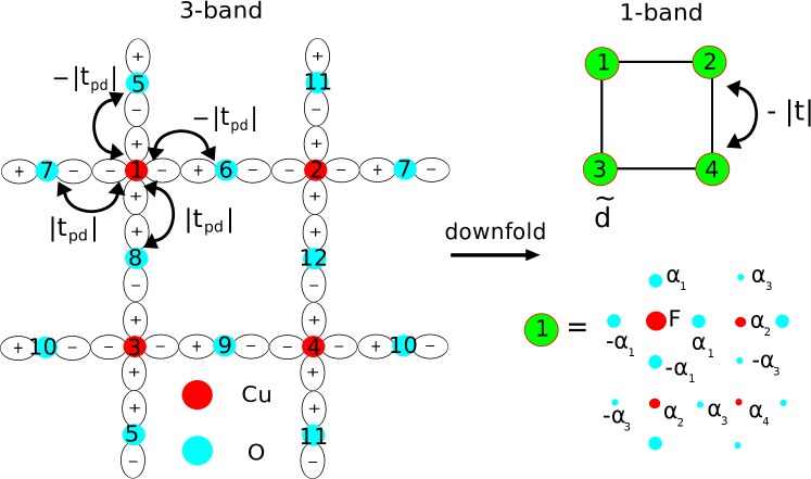
Figure 2: Schematic for downfolding the three-band Hubbard model on the $2\times 2$ cell to the one-band Hubbard model. The oxygen orbitals are eliminated to give “dressed” $d$-like orbitals of the one-band model, with modified hopping and interaction parameters. The relationship between the $\tilde{d}$ and the copper and oxygen orbitals is encoded by a linear transformation which is parameterized by $\alpha_{1}$, $\alpha_{2}$, $\alpha_{3}$, $\alpha_{4}$ and $F$ (see Appendix for more details). Here the diameter of the circles has been shown to be proportionate to the magnitude of $F$ or $\alpha_{i}$.

It is our objective to determine what one-band Hubbard model [Eq. (10)] “best” describes the three-band data. The effective d-like orbitals $\tilde{d}_{i,\eta}$, that enter the low energy description are mixtures of copper and oxygen orbitals; this optimal transformation also remains an unknown. Thus the model determination involves two aspects (1) what are the composite objects that give a compact description of the low energy physics? and (2) given this choice what are the effective interactions between them? (A similar problem was posed and solved by one of us in the context of spin systems Changlani_percolation .) In addition, the best effective Hamiltonian description depends on the energy scale of interest. All these issues will be addressed in the remainder of the section.

We begin by encoding the relationship between the bare and effective operators as a linear transformation ${\bf T}$,

$$\tilde{d}_{i,\eta}=\sum_{j}T_{ij}c_{j,\eta}$$ (12)

where $c_{j,\eta}$ is the hole (destruction) operator and refers to either the bare $d$ or $p$ orbitals. Further generalizations of this relationship (for example, including higher body terms) are also possible, but have not been considered here. For the $2\times 2$ unit cell T is a $4\times 12$ matrix, which we parameterize by four distinct parameters. These correspond to mixing of a copper orbital with nearest neighbor oxygens ($\alpha_{1}$), nearest neighbor coppers ($\alpha_{2}$), next-nearest neighbor oxygens ($\alpha_{3}$) and next-nearest neighbor coppers ($\alpha_{4}$) as shown schematically in Figure 2. The explicit form of ${\bf T}$ after accounting for the symmetries of the lattice has been written out in the Appendix. These parameters are optimized to minimize a certain cost function, which will be explained shortly.

All RDMs in the three-band and one-band descriptions are also related via ${\bf T}$; the ones that we focus on are evaluated in eigenstate $s$ and are given by,

$$\langle{\tilde{d}_{i,\eta}}^{\dagger}\tilde{d}_{j,\eta}\rangle_{s} = \sum_{mn}T^{*}_{im}\langle{c_{m,\eta}}^{\dagger}c_{n,\eta}\rangle_{s}T_{jn}\,,$$ (13a)

$$\langle\tilde{n}_{i,\uparrow}\tilde{n}_{i,\downarrow}\rangle_{s} = \sum_{jkmn}T^{*}_{ij}T^{*}_{im}\langle{c_{j,\uparrow}}^{\dagger}{c_{m,\downarrow}}^{\dagger}c_{n,\downarrow}c_{k,\uparrow}\rangle_{s}T_{in}T_{ik}\,.$$ (13b)

We optimize ${\bf T}$ by demanding two conditions be satisfied, (1) the effective orbitals ($\tilde{d}_{i,\eta}$) are orthogonal to each other i.e. $\Big{(}{\bf T}{\bf T}^{\dagger}\Big{)}_{mn}=\delta_{mn}$ and (2) the sum of all diagonal entries (trace) of the 1-RDM of the effective orbitals for all low energy eigenstates equals the number of electrons of a given spin i.e. $\sum_{i}\sum_{\eta}\langle{\tilde{d}_{i,\eta}}^{\dagger}\tilde{d}_{i,\eta}\rangle_{s}=N_{\eta}$. These conditions are enforced by minimizing a cost function,

$$C=\sum_{s}\sum_{\eta}\Big{(}\sum_{i}\langle\tilde{d}_{i,\eta}^{\dagger}\tilde{d}_{i,\eta}\rangle_{s}-N_{\eta}\Big{)}^{2}+\sum_{mn}(\Big{(}{\bf T}{\bf T}^{\dagger}\Big{)}_{mn}-\delta_{mn})^{2}\,.$$ (14)

For the $2\times 2$ cell, $N_{\uparrow}=N_{\downarrow}=2$ and $i=1,2,3,4$. The number of states $s$ was varied from three to six, depending on the energy window of interest.

Figure 3 shows regimes of the three-band model where the lowest six eigenstates are separated from the higher energy manifold; the fourth and fifth eigenstates are degenerate. In the large $U_{d}$ limit, charge fluctuations are suppressed and these six states correspond to the Hilbert space of $4\choose 2$ states of the effective spin model in its $S_{z}=0$ sector. These states have primarily d-like character, an aspect we will verify in this section. The eigenstates outside of this manifold involve p-like excitations which the one-band model is not designed to capture.

We chose the lowest three eigenstates of the three-band model for minimizing the cost in Eq. (14). The four dimensional space of parameters of ${\bf T}$ was scanned for this purpose. The corresponding trace and orthogonality conditions are simultaneously satisfied with only small deviations, confirming the validity of Eq. (12). Importantly, the 1-RDM elements in the transformed basis corresponding to nearest neighbors $\langle\tilde{d}_{1}^{\dagger}\tilde{d}_{2}\rangle_{s}$ already provide estimates for $U/t$ of the effective model. Since the exact knowledge of the corresponding eigenstates of the one-band Hubbard model is available for arbitrary $U/t$ by exact diagonalization, we directly look up the $U/t$ with the same 1-RDM value. These estimates complement the one obtained by DMD which was carried out with the same three low-energy eigenstates, using their energies and the computed values of $\langle\tilde{d}_{1}^{\dagger}\tilde{d}_{2}\rangle_{s}$ and $\langle\tilde{n}_{i,\uparrow}\tilde{n}_{i,\downarrow}\rangle_{s}$ from Eqs. (13a) and (13b).   A representative example of our results for $U_{d}/t_{pd}=8$ and $\Delta/t_{pd}=3$ has been discussed in the Appendix.

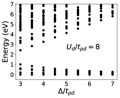
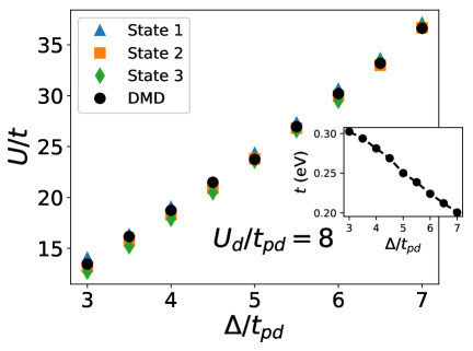
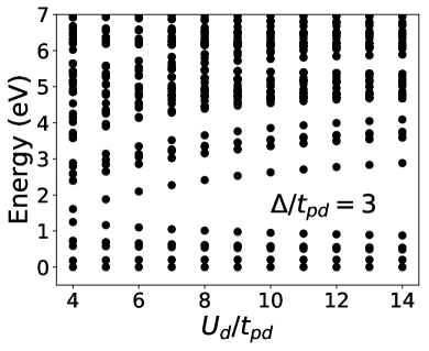
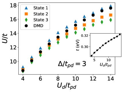
Figure 3: Downfolding of a three-band Hubbard model to an effective one-band Hubbard model of d-like orbitals. Panels (A) and (C) show the low energy spectra of the three-band model (relative to the corresponding ground state) for the cases of (A) fixed $U_{d}/t_{pd}=8$ and varying $\Delta/t_{pd}$ and (C) fixed $\Delta/t_{pd}=3$ and varying $U_{d}/t_{pd}$. In all cases, $t_{pd}$ is set to be $1.3$ eV. Panels (B) and (D) show the downfolded parameters for the one-band model corresponding to the three-band parameter choices in (A) and (C) respectively. The one-band $U/t$ values were obtained either by comparing $\langle\tilde{d}_{1}^{\dagger}\tilde{d}_{2}\rangle_{s}$ with the corresponding one-band model eigenstates or by the DMD procedure using the lowest three eigenstates. The insets show $t$ obtained from DMD.

Some trends in the one-band description are explored in Figure 3 by monitoring the downfolded parameters as a function of varying $\Delta/t_{pd}$ and $U_{d}/t_{pd}$. For example, when $U_{d}/t_{pd}=8$ is fixed and $\Delta/t_{pd}$ is increased, we find that the effective hopping $t$ decreases and $U/t$ increases. This is physically reasonable since an increasing difference in the single particle energies of the copper and oxygen orbitals makes it energetically unfavorable for holes to hop between the two orbitals. When $\Delta/t_{pd}=3$ is fixed and $U_{d}/t_{pd}$ is increased, $U/t$ increases. As one mechanism of avoiding the large $U_{d}$, the copper orbitals are forced to hybridize more with the oxygen ones; on the other hand, hole delocalization is suppressed in a bid to maintain mostly one hole per $\tilde{d}$ due to the larger $U/t$. The net result of these effects is that the $t$ also increases.

An important check for the one-band model is its ability to reproduce the low energy gaps of the three-band model; these have been compared in Figure 4. For the case of $\Delta/t_{pd}=3$, we observe that for all $U_{d}/t_{pd}$ the lowest three eigenstates were reproduced well. This model also reproduces the states outside of the DMD energy window, although with slightly larger errors. Similar trends are seen for the case of $\Delta/t_{pd}=5$, with the noticeable difference being that the energy error of the highest state has reduced. This also reflects that the parameters obtained from DMD are, in general, dependent on the energy window of interest, a point which we will highlight shortly by investigating it systematically.

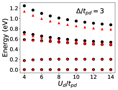
(A)                                  (B)

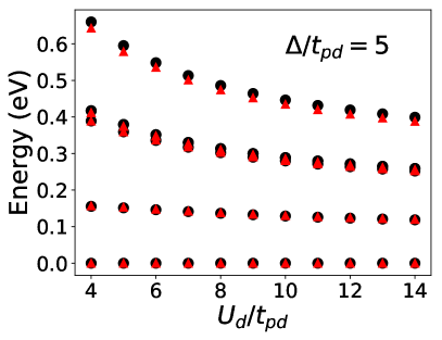
Figure 4: Comparison of energy spectra of the original three-band model (black circles) and the effective one-band model (red triangles). The three-band model is on the $2\times 2$ cell. (A) and (B) show the energy spectra for different parameter sets of the three-band model: (A) $\Delta/t_{pd}=3$ and various $U_{d}/t_{pd}$; (B) $\Delta/t_{pd}=5$ and various $U_{d}/t_{pd}$. In all cases, $t_{pd}=1.3$ eV.

A promise of downfolding is the reduction of the size of the effective Hilbert space; allowing simulations of bigger unit cells to be carried out. To show that this actually works well in practice for the three-band case, we consider the $2\sqrt{2}\times 2\sqrt{2}$ square unit cell, comprising of 8 copper and 16 oxygen orbitals. For representative test cases, we performed exact diagonalization calculations at half filling; the Hilbert space comprises of 112,911,876 basis states. Roughly 200 Lanczos iterations were carried out, enabling convergence of the lowest four energies. We compared the lowest gaps with the corresponding calculation on the one-band model on the same square geometry, with a Hilbert space size of only 4,900, using the downfolded parameters obtained from the smaller $2\times 2$ cell.

Our results are summarized in Figure 5. Panel (A) shows the six representative parameter sets of the three-band model and the corresponding downfolded one-band parameters. Panels (B) and (C) show the lowest three energy gaps for representative values of $U_{d}/t_{pd}=4,8,12$ for $\Delta/t_{pd}=3$ and $\Delta/t_{pd}=5$ respectively. In all cases, the agreement between the three-band and one-band models is remarkably good. The energy gap error of the lowest gap is within $0.0004$ eV (1% relative error). The largest error in the third gap is of the order of $0.005$ eV (3% relative error). These results indicate the reliability of the downfolding procedure and highlight its predictive power.

                          (A)

  $\Delta/t_{pd}$ $U_{d}/t_{pd}$ $t$ $U/t$ 3.0 4.0 0.2839 8.698 3.0 8.0 0.3025 13.45 3.0 12.0 0.3155 16.58 5.0 4.0 0.2326 15.08 5.0 8.0 0.2501 23.75 5.0 12.0 0.2647 29.89

                       (B)

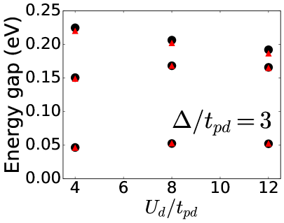
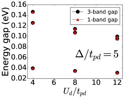
                       (C)

Figure 5: Multiscale prediction of the effective one-band model. (A) shows the parameters of the effective one-band model obtained from DMD on a small cell, the 4-copper ($2\times 2$) cell. These parameters were then directly used to predict the energy spectra of a larger cell, the 8-copper ($2\sqrt{2}\times 2\sqrt{2}$) cell. (B) and (C) show the predicted spectra (red triangles) in comparison to the exact spectra (black circles) of the three-band model of different parameters (different $\Delta/t_{pd}$ and $U_{d}/t_{pd}$ where $t_{pd}=1.3$ eV).

Until this point, all our results focused on downfolding using only the lowest three eigenstates of the $2\times 2$ cell. We now explore the effect of increasing the energy window, by including higher eigenstates, using our test example of $U_{d}/t_{pd}=8$ and $\Delta/t_{pd}=3$. To do so, we now use all six low energy eigenstates for optimizing the cost function in Eq. (14). We find similar (but not exactly the same) values of $\alpha_{i}$ compared to the case when only the three lowest states were used. The fact that a solution with small cost can be attained confirms our expectation that the entire low energy space of six states is consistently described by a set of $\tilde{d}_{i}$ operators.

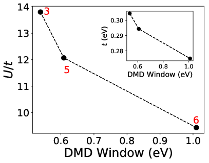
(A)                               (B)

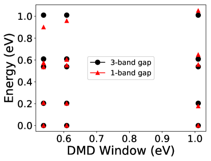
Figure 6: Dependence of the downfolding parameters on the chosen low energy manifold. (A) shows the variation of downfolded parameters $U/t$ and $t$ (inset) with low energy manifolds of different energy windows (corresponding to 3,5 and 6 low energy eigenstates); (B) shows the energy spectra of the effective one-band model (red triangles) in comparison to the spectra of the original three-band model (black circles). The three-band Hubbard model is on the $2\times 2$ cell with $U_{d}/t_{pd}=8$, $\Delta/t_{pd}=3$, and $t_{pd}=1.3$.

However, as Figure 6(A) shows, the estimates of $U/t$ and $t$ depend on how many eigenstates are used in the DMD procedure. This is because the DMD aims to provide the one-band description that best describes all states in a given window. If the model is not perfect within a given energy window, an energy dependent model is expected, consistent with the renormalization group perspective. For our test example, increasing the number of eigenstates from three to six changed $U/t$ from $13.8$ to $9.44$ and $t$ from $0.3045$ to $0.2750$ eV.

The features associated with the energy dependence are further confirmed in Figure 6(B). which shows a comparison of energy gaps of the three-band and downfolded one-band model on the $2\times 2$ cell. When only three states are used, the one-band (nearest neighbor) Hubbard model is insufficient for accurately describing states outside the window. When all six states are used, the DMD tries to minimize the error of the largest energy gap at the cost of errors in the smaller energy gaps. One could of course choose a different parameterization, say with additional next nearest neighbor $t^{\prime}$, for which is may be possible to reduce this energy dependence significantly and thus have a model that describes the smaller and larger energy scales equally well.

III.2 One dimensional hydrogen chain

We now move on to one of the simplest extended ab initio systems, a hydrogen chain in one dimension with periodic boundary conditions. The one-dimensional hydrogen chain has been used as a model for validating a variety of modern ab initio many-body methods H10_Simons . We consider the case of $10$ atoms with periodic boundary conditions and work in a regime where the inter-atomic distance $r$ is in the range $1.5-3.0$ Å, such that the system is well described in terms of primarily $s$-like orbitals.

For a given $r$, we first obtain single-particle Kohn-Sham orbitals from a set of spin-unrestricted and spin-restricted DFT-PBE calculations. The localized orbital basis upon which the RDMs (descriptors) are evaluated is obtained by generating intrinsic atomic orbitals (IAO) knizia_intrinsic_2013 from the Kohn-Sham orbitals orthogonalized using the Löwdin procedure (see Figure 7). These are the orbitals that enter the one-band Hubbard Hamiltonian. Then, to generate a database of wavefunctions needed for the DMD, we produce a set of Slater-Jastrow wavefunctions consisting of singles and doubles excitations to the Slater determinant:

$$|s\rangle= e^{J}\Big{[}a^{\dagger}_{i\eta}a_{k\eta}|KS\rangle\Big{]}\,,$$ (15a)

$$|d\rangle= \>e^{J}\Big{[}a^{\dagger}_{i\eta}a^{\dagger}_{j\eta^{\prime}}a_{k\eta^{\prime}}a_{l\eta}|KS\rangle\Big{]},$$ (15b)

where $|KS\rangle$ is the Slater determinant of occupied Kohn-Sham orbitals, $\eta\neq\eta^{\prime}$ are spin indices, and $a_{i}^{\dagger}$ ($a_{i}$) is a single-electron creation (destruction) operator corresponding to a particular Kohn-Sham orbital. The $k,l$ indices label occupied orbitals in the original Slater determinant, while $i,j$ are virtual orbitals. $e^{J}$ is a Jastrow factor optimized by minimizing the variance of the local energy.

We compute the energies (expectation values of the Hamiltonian) and the RDMs for each wave function within DMC. By computing the trace of the resulting 1-RDMs, we verify that all the electrons present in the system are represented within the localized basis of $s$-like orbitals. If the trace of the 1-RDM deviates from the nominal number of electrons for a particular state by more than some chosen threshold - 2% in this example - it indicates that some orbitals are occupied ($2s$- or $2p$-like orbitals for hydrogen) that are not represented within the localized IAO basis used for computing the descriptors. Hence, these states do not exist within the $\mathcal{LE}$ space, and cannot be described by a one-band $s$-orbital model. We exclude such states from the wave function set. The acquired data is then used in DMD to downfold to a one-band Hubbard Hamiltonian.

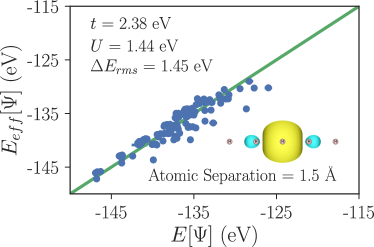
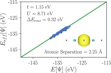
(A)               (B)

Figure 7: Reconstructed model energy ($E_{eff}[\psi]$) versus DMC energy ($E[\psi]$) for the H₁₀ chain at (A) 1.5 Å  and (B) 2.25 Å . The energy range of excitations narrows significantly for larger interatomic separation. Insets show the intrinsic atomic orbitals which constitute the one-body space which was used for calculating the reduced density matrices (descriptors).

Figure 7 shows the fitting results of the energy functional $E[\Psi]$ within the sampled $\mathcal{LE}$ for two representative distances (1.5 and 2.25Å). As we can see, the model $E_{eff}[\Psi]$ reproduces the ab initio $E[\Psi]$ up to certain error that decreases with atomic separation. That is, the fitted Hubbard model provides a more accurate description as separation distance increases, and the system becomes more atomic-like.

Figure 8 shows the fitted values of the downfolding parameters $t$ and $U/t$ at various distances. $t$ decreases as the interatomic distance increases, and the value of $U/t$ increases. The single-band Hubbard model qualitatively captures how the system approaches the atomic limit, in which $t$ becomes zero.

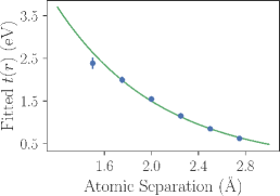
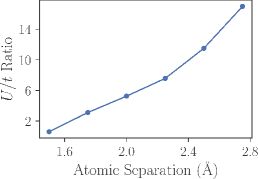
(A)          (B)          (C)

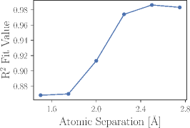
Figure 8: (A) The one-body hopping $t$ parameter as a function of interatomic distance for the periodic H₁₀ chain, obtained from a fitted $U$-$t$ model. $t$ declines to zero as $r$ increases. (B) The ratio $U/t$ for the fitted parameter values as a function of interatomic separation. The ratio is small at lower bond-lengths, where $t$ is more relevant in describing the system, and larger at longer bond-lengths, where inter-site hopping is less significant. (C) The R² fit parameters obtained from fitting the $U$-$t$ model to the H₁₀ chain, as a function of interatomic separation.

The R² values obtained from fitting the descriptors to the ab initio energy [see Figure 8(C)] also show that the single-band Hubbard model is a good description of the system at large distances, but not at small distances. This is primarily because the dynamics of other degrees of freedom (e.g. $2s$ and $2p$ orbitals) become important to the low energy spectrum at small distances. Other interaction terms beyond the on-site Hubbard $U$, such as nearest-neighbor Coulomb interactions and Heisenberg coupling, can also become significant. Without including higher orbitals or additional many-body interaction terms, the model gives rise to an incorrect insulator state at small distances. Conversely, at larger separations ($r>1.8$Å), where the system is in an insulator phase Stella2011 , the model provides a better description.

III.3 Graphene and hydrogen honeycomb lattice

Our third example highlights the role of the high energy degrees of freedom not present in the low energy description but which are instrumental in renormalizing the effective interactions. We demonstrate this by considering the case of graphene, and by comparing it to artificially constructed counterparts without the high energy electrons. Although many electronic properties of graphene can be adequately described by a noninteracting tight-binding model of $\pi$ electrons Castro2009 , electron-electron interactions are crucial for explaining a wide range of phenomena observed in experiments Kotov2012 . In particular, electron screening from $\sigma$ bonding renormalizes the low energy plasmon frequency of the $\pi$ electrons Zheng2016 . In fact a system of $\pi$ electrons with bare Coulomb interactions has been shown to be an insulator instead of a semimetal DrutPRL2009 ; DrutPRB2009 ; Smith2014 ; Zheng2016 . Using DMD, we demonstrate how the screening effect of $\sigma$ electrons is manifested in the low energy effective model of graphene.

In order to disentangle the screening effect of $\sigma$ electrons from the bare interactions between $\pi$ electrons, we apply DMD to three different systems, graphene, $\pi$-only graphene, and a honeycomb lattice of hydrogen atoms. In the $\pi$-only graphene, the $\sigma$ electrons are replaced with a static constant negative charge background. The role of $\sigma$ electrons is then clarified by comparing the effective model Hamiltonians of these two systems. The hydrogen system we study has the same lattice constant $a=2.46$ Å as graphene, which has a similar Dirac cone dispersion as graphene Zheng2016 .

By constructing the one-body space by Wannier localizing Kohn-Sham orbitals obtained from DFT calculations (see Figure 9), we verify that the low energy degrees of freedom correspond to the $\pi$ orbitals in graphene and its $\pi$-only system and $s$ orbitals in hydrogen; these enter the effective one-band Hubbard model description in Eq. (10). Due to the vanishing density of states at the Fermi level, the Coulomb interaction remains long-ranged, in contrast to usual metals where the formation of electron-hole pairs screens the interactions strongly Zheng2016 . However, for certain aspects, the long ranged part can be considered as renormalizing the onsite Coulomb interaction $U$ at low energy Schuler2013 ; Changlani2015 .

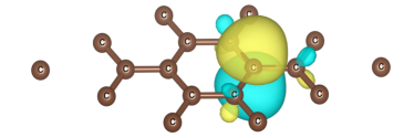
(A)       (B)

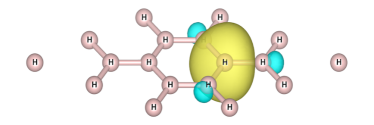
Figure 9: Wannier orbitals constructed from Kohn-Sham orbitals: (A) graphene $\pi$ orbital; (B) hydrogen $s$ orbital.

To estimate the one-band Hubbard parameters, we used the DMD method using a set of 50 Slater-Jastrow wave functions that correspond to the electron-hole excitations within the $\pi$ channel for the graphene systems or $s$ channel for the hydrogen system. In particular, for graphene, the Slater-Jastrow wave functions are constructed from occupied $\sigma$ bands and occupied $\pi$ bands, whereas for $\pi$-only graphene, Slater-Jastrow wave functions constructed from occupied $\pi$ Kohn-Sham orbitals of graphene. The ab initio simulations were performed on a $3\times 3$ cell (32 carbons or hydrogens) and the energy and RDMs of these wave functions were evaluated with VMC. The error bars on our downfolded parameters are estimated using the jackknife method Jackknife1981 . The results from our calculations are summarized in Figure 10.

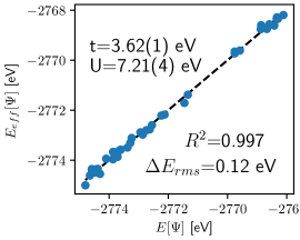
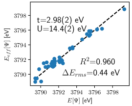
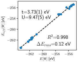
(A)              (B)              (C)

Figure 10: Comparison of ab initio ($E[\psi]$) and fitted energies ($E_{eff}[\psi]$) of the 3$\times$3 periodic unit cell of graphene and hydrogen lattice: (A) graphene; (B) $\pi$-only graphene; (C) hydrogen lattice.

We find that the one-band Hubbard model describes graphene and hydrogen very well, as is seen from the fact that $R^{2}$ is closed to 1 for the fits. Our fits are shown in Figure 10. For both graphene and hydrogen, $U/t$ is smaller than the critical value of the semimetal-insulator transition $(U/t)_{c}\approx 3.8$ for the honeycomb lattice Sorella2012 , which is consistent with both systems being semimetals. The two systems indeed have similar hopping constant $t$, consistent with the fact that they have similar Fermi velocities at the Dirac point. However, the difference in their high energy structure manifests itself as differently renormalized electron-electrons interactions, explaining the difference in $U$. Most prominently, the $\pi$-only system has much larger $U/t$ ($\sim 4.9$) compared to graphene, which is large enough to push it into the insulating (antiferromagnetic) phase. Thus, downfolding shows the clear significance of $\sigma$ electrons in renormalizing the effective onsite interactions of the $\pi$ orbitals,making graphene a weakly interacting semimetal instead of an insulator.

III.4 FeSe diatomic molecule

Transition metal systems are often difficult to model due to the many orbital and possibly magnetic descriptors introduced by $d$ electrons. This is seen in the proliferation of models for transition metals, which include terms like spin-spin coupling, spin-orbital coupling, hopping, Hund’s like coupling, and so on. Models containing all possible descriptors are unwieldy, and it is difficult to determine which degrees of freedom are needed for a minimal model to reproduce an interesting effect. Transition metal systems are challenging to describe using most electronic structure methods because of the strong electron correlations and multiple oxidation states possible in these systems. Fixed-node DMC has been shown to be a highly accurate method on transition metal materials in improving the description of the ground state properties and energy gaps Foyevtsova2014 ; Wagner_Abbamonte ; Zheng2015 ; Wagner2016 . In this section, we apply DMD using fixed-node DMC to quantify the importance of various interactions in a FeSe diatomic molecule with a bond length equal to that of the iron based superconductor, FeSe kumar_crystal_2010 , in order to help identifying the descriptors that may be relevant in the bulk material.

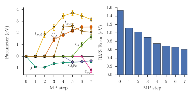
Figure 11: (Left) Parameter values for each fit generated in the MP algorithm, labeled at the step where they are included in the model. A zero value indicates that parameter is not yet added to the model. The sign of $J$ is consistent with Hund’s rules, and the signs of $t_{\sigma,d}$ and $t_{\sigma,s}$ are consistent with Se being located in positive $z$ with respect to Fe. (Right) RMS error of each model generated by MP as the algorithm includes parameters. The RMS error of the largest model considered was 0.61 eV.

We considered a low-energy space spanned by the Se $4p$, Fe $3d$, and Fe $4s$ orbitals. We sampled singles and doubles excitations from a reference Slater determinant of Kohn-Sham orbitals taken from DFT calculations with PBE0 functional with total spin 0, 2, and 4, which were then multiplied by a Jastrow factor and further optimized using fixed-node DMC. After this procedure, 241 states were within a low energy window of 8 eV. Of these, eight states had a significant iron $4p$ component, which excludes them from the low-energy subspace. This leaves us with 233 states in the low-energy subspace.

We consider a set of 21 possible descriptors consisting of local operators on the iron $4s$, iron $3d$ states, and selenium $4p$ states, which is a total of 9 single-particle orbitals. We use the same IAO construction as Section III.2 to generate the basis for these operators. At the one-body level, we consider orbital energy descriptors:

$$\epsilon_{s}n_{s}, \epsilon_{\pi,\mathrm{Se}}(n_{p_{x}}+n_{p_{y}}), \epsilon_{z}n_{p_{z}},$$

$$\epsilon_{z^{2}}n_{d_{z^{2}}}, \epsilon_{\pi,\mathrm{Fe}}(n_{d_{xz}}+n_{d_{yz}}). \epsilon_{\delta}(n_{d_{xy}}+n_{d_{x^{2}-y^{2}}}),$$ (16)

and the symmetry-allowed hopping terms:

$$t_{\sigma,d}\sum_{\eta}\left(c_{d_{z^{2}},\eta}^{\dagger}c_{p_{z},\eta}+\text{h.c.}\right), t_{\sigma,s}\sum_{\eta}\left(c_{s,\eta}^{\dagger}c_{p_{z},\eta}+\text{h.c.}\right), t_{\pi}\sum_{\eta}\left(c_{d_{xz},\eta}^{\dagger}c_{p_{x},\eta}+c_{d_{yz},\eta}^{\dagger}c_{p_{y},\eta}+\text{h.c.}\right).$$ (17)

As before, $\eta$ represents the spin index. At the two-body level, we consider Hubbard interactions:

$$U_{p}\sum_{i\in p}n_{i,\uparrow}n_{i,\downarrow}, U_{d,\delta}\sum_{i\in\{d_{xy},d_{x^{2}-y^{2}}\}}n_{i,\uparrow}n_{i,\downarrow},$$

$$U_{d}\sum_{i\in d}n_{i,\uparrow}n_{i,\downarrow}, U_{d,\pi}\sum_{i\in\{d_{xz},d_{yz}\}}n_{i,\uparrow}n_{i,\downarrow}, U_{d_{z^{2}}}n_{d_{z^{2}},\uparrow}n_{d_{z^{2}},\downarrow},$$ (18)

where $p$ refers to the Se-$4p$ orbitals and $d$ refers to the Fe-$3d$ orbitals. Importantly, we also account for the Hund’s coupling terms for the iron atom:

$$J\sum_{\begin{subarray}{c}i\neq j\\ i,j\in d\end{subarray}}S_{i}\cdot S_{j}, J_{\delta}S_{d_{xy}}\cdot S_{d_{x^{2}-y^{2}}}, J_{\delta,d_{z^{2}}}(S_{d_{xy}}+S_{d_{x^{2}-y^{2}}})\cdot S_{d_{z^{2}}},$$

$$J_{\pi}S_{d_{xz}}\cdot S_{d_{yz}}, J_{\pi,d_{z^{2}}}(S_{d_{xz}}+S_{d_{yz}})\cdot S_{d_{z^{2}}}. J_{\pi,\delta}(S_{d_{xz}}+S_{d_{yz}})\cdot(S_{d_{xy}}+S_{d_{x^{2}-y^{2}}}),$$ (19)

Finally, we also add a nearest neighbor Hubbard interaction: $V\sum_{i\in p,j\in d}n_{i}n_{j}$.

To generate a minimal description of the system, we employed a matching pursuit (MP) method MP_Zhang1993 . MP chooses to add descriptors based on their correlation with the residual of the linear fit. We started with a model that only consists of $E_{0}$. The Hund’s coupling descriptor [first term in Eq. (III.4)] has the largest correlation coefficient with the residual fit, so it is added first. The fact that the Hund’s coupling is chosen first in MP is consistent with the several studies in the literature, which find a prominent Hund’s coupling can explain some of the properties of bulk FeSe. demedici_hunds_2011 ; de_medici_janus-faced_2011 ; georges_strong_2013 ; busemeyer_competing_2016 . Next, MP includes the descriptor that correlates most strongly with the residuals of this first minimal model, in this case the hopping between $d$ and $p$ $\sigma$-symmetry orbitals. We repeated this procedure until the RMS error did not improve more than 0.05 eV upon adding a new parameter. This criterion was chosen to strike a balance between the complexity of the model and the accuracy in reproducing the sample set.

The following model was produced:

$$H_{eff} = \epsilon_{\delta,\mathrm{Fe}}(n_{d_{xy}}+n_{d_{x^{2}-y^{2}}})+\epsilon_{s}n_{s}+\epsilon_{z}n_{p_{z}}$$ (20)

$$+t_{\sigma,d}\sum_{\eta}\left(c_{d_{z^{2}},\eta}^{\dagger}c_{p_{z},\eta}+\text{h.c.}\right)+t_{\sigma,s}\sum_{\eta}\left(c_{s,\eta}^{\dagger}c_{p_{z},\eta}+\text{h.c.}\right)$$

$$+U_{d}\sum_{i\in d}n_{i,\uparrow}n_{i,\downarrow}+J\sum_{\begin{subarray}{c}i\neq j\\ i,j\in d\end{subarray}}S_{i}\cdot S_{j}+E_{0}.$$

As before, $\eta$ is the spin index and $i$ is the orbital index, and $d$ is the set of iron $3d$ orbitals, as above. $E_{0}$ is an overall energy shift, also included as a fit parameter. The parameter values and corresponding error of each model produced by MP are shown in Figure 11. Note that all parameters may change at each step because the entire model is refitted when an addition parameter is included in each iteration. The parameters are smoothly varying with the inclusion of new parameters, and they take the correct signs based on symmetry (where applicable). The RMS error decreases with each additional parameter, but less so as the algorithm appends additional parameters. Eventually the diminishing improvements do not merit the additional complexity of more parameters.

IV Conclusion and Future prospects

The density matrix downfolding (DMD) technique uses data derived from low-energy approximate solutions to a high energy Hamiltonian to systematically determine an effective Hamiltonian that describes the low-energy behavior of the system. It is based on several rather simple proofs which occupy a role similar to the variational principle; they allow us to know which effective models are closer to the correct solution than others. The method is very general and does not require a quasiparticle picture to apply, and neither does it have double-counting issues. It treats all interactions on an equal footing, so hopping parameters are naturally modified by interaction parameters and so on. While most of the applications have used the first principles quantum Monte Carlo method to obtain the low-energy solutions, the method is completely general and can be used with any solution method that can produce high quality energy and reduced density matrices. We have discussed several examples to present the conceptual and algorithmic aspects of DMD.

The resultant lattice model can be efficiently and accurately solved for large system sizes LeBlanc_PRX using techniques designed and suited for small local Hilbert spaces; these include exact or selected diagonalization DeRaedt ; Tubman_selci ; Holmes_Tubman_Umrigar , density matrix renormalization group (DMRG) White1992 , tensor networks PEPS ; Changlani_CPS ; NeuscammanCPS , dynamical mean field theory (DMFT) Kotliar2006 , density matrix embedding (DMET) DMET_2012 and lattice QMC methods Scalapino ; Trivedi_Ceperley ; Zhang_AFQMC ; Sandvik_loops ; Prokofiev ; Booth2009 ; SQMC ; Holmes_Changlani_Umrigar ; Booth2013 . These methods have also been used to obtain excited states, dynamical correlation functions and thermal properties, that have been difficult to obtain in ab initio approaches.

DMD, though conceptually simple, is still a method in its development stages, with room for algorithmic improvements and new applications. Advances in the field of inverse problems Berg2017 could be incorporated into DMD to mitigate the problems associated with optimization and over-fitting. Here we briefly outline some aspects that need further research:

1. The wave function database ($\ket{\Psi}\in\mathcal{LE}$): The DMD method relies crucially on the availability of a low energy space of ab initio wave functions. While these wave functions do not have to be eigenstates, automating their construction remains challenging and realistically requires knowledge of the physics to be described.

2. Optimal choice of basis functions. The second-quantized operators in the effective Hamiltonian correspond to a basis in the continuum. The quality of the model depends on the basis describing the changes between low-energy wave functions accurately.

3. Form of the low energy model Hamiltonian. While the exact effective Hamiltonian is unique, there may be many ways of approximating it with varying levels of compactness and accuracy.

The advantage of the DMD framework is that all these can be resolved internally. Given a good sampling of $\mathcal{LE}$, (2) and (3) can be resolved using regression. Given that (2) and (3) are correct or near correct, then (1) can be resolved by finding binding planes, as noted in Section II. The method thus has a degree of self consistency; it will return low errors only when 1-3 are correct.

We have shown applications to strongly correlated models (3-band), ab initio bulk systems hydrogen chain and graphene, and a transition metal molecule FeSe. The technique is on the verge of being applied to transition metal bulk systems; there are no major barriers to this other than a polynomially scaling computational cost and the substantial amount of work involved in parameterizing and fitting models to these systems. Looking into the future, we anticipate that this technique can help with the definition of a correlated materials genome–what effective Hamiltonian best describes a given material is highly relevant to its behavior.

Author Contributions

HJC, HZ and LKW conceived the initial DMD ideas and designed the project and organization of the paper. All authors contributed to the theoretical developments and various representative ab initio and lattice examples. All authors contributed to the analysis of the data, discussions and writing of the manuscript. LKW oversaw the project. HJC and HZ contributed equally to this work.

Appendix

In Section III.1 we discussed parameterizing the transformation ${\bf T}$ as a $4\times 12$ matrix for the $2\times 2$ unit cell, in terms of $\alpha_{1}$, $\alpha_{2}$, $\alpha_{3}$ and $\alpha_{4}$. Using the numbering of the orbitals corresponding to Figure 2, the explicit form of ${\bf T}$ is,

$${\bf T}=\left(\begin{array}[]{cccccccccccc}F&\alpha_{2}&\alpha_{2}&\alpha_{4}&\alpha_{1}&\alpha_{1}&-\alpha_{1}&-\alpha_{1}&\alpha_{3}&-\alpha_{3}&\alpha_{3}&-\alpha_{3}\\ \alpha_{2}&F&\alpha_{4}&\alpha_{2}&\alpha_{3}&-\alpha_{1}&\alpha_{1}&-\alpha_{3}&-\alpha_{3}&\alpha_{3}&\alpha_{1}&-\alpha_{1}\\ \alpha_{2}&\alpha_{4}&F&\alpha_{2}&-\alpha_{1}&\alpha_{3}&-\alpha_{3}&\alpha_{1}&\alpha_{1}&-\alpha_{1}&-\alpha_{3}&\alpha_{3}\\ \alpha_{4}&\alpha_{2}&\alpha_{2}&F&-\alpha_{3}&-\alpha_{3}&\alpha_{3}&\alpha_{3}&-\alpha_{1}&\alpha_{1}&-\alpha_{1}&\alpha_{1}\\ \end{array}\right)\,,$$ (25)

where we have defined $F\equiv\sqrt{1-4{\alpha_{1}}^{2}-2{\alpha_{2}}^{2}-4{\alpha_{3}}^{2}-{\alpha_{4}}^{2}}$.

A concrete and representative example of our results, shown in Section III.1 for the $2\times 2$ cell, is explained for the case of $U_{d}/t_{pd}=8$ and $\Delta/t_{pd}=3$. The first task was to obtain the optimal transformation ${\bf T}$ for which the lowest three eigenstates ($s=1,2,3$) of the three-band model were used for computing the cost in Eq. (14). The minimum of the cost was determined by a brute force scan in the four dimensional space of $\alpha$’s and using a linear grid spacing of $0.002$ found $\alpha_{1}=0.216$, $\alpha_{2}=0.042$, $\alpha_{3}=0.018$ and $\alpha_{4}=0.016$. The two terms in the cost i.e. the trace and orthogonality conditions are individually satisfied to a relative error of less than 0.5 percent.

$\langle c_{i}^{\dagger}c_{j}\rangle_{s}$ and $\langle{c_{j,\uparrow}}^{\dagger}{c_{m,\downarrow}}^{\dagger}c_{n,\downarrow}c_{k,\uparrow}\rangle_{s}$ were computed from the exact knowledge of the three-band model eigenstates and hence $\langle{\tilde{d}_{i,\eta}}^{\dagger}\tilde{d}_{j,\eta}\rangle_{s}$ and $\langle\tilde{n}_{i,\uparrow}\tilde{n}_{i,\downarrow}\rangle_{s}$ are obtained once the optimal ${\bf T}$ has been determined. As mentioned in the main text, the value of $\langle\tilde{d}_{1,\eta}^{\dagger}\tilde{d}_{2,\eta}\rangle_{s}$ provides estimates for $U/t$ of the effective model by direct comparison of its value to that in the corresponding eigenstate in the one-band model. For our test example, the absolute values of $\langle\tilde{d}_{1,\uparrow}^{\dagger}\tilde{d}_{2,\uparrow}\rangle_{s}$ in states $s=1,2,3$ are approximately $0.159$, $0.142$ and $0.084$ respectively which correspond to $(U/t)_{1}\approx 14.1$, $(U/t)_{2}\approx 13.2$, $(U/t)_{3}\approx 12.7$. Performing DMD with the three eigenenergies and their calculated RDMs gave $t=0.3025$ eV and $U/t=13.45$; the latter in the correct range of the other estimates.

References

- [1] Kenneth G. Wilson. The renormalization group: Critical phenomena and the kondo problem. Reviews of Modern Physics, 47(4):773–840, October 1975.
- [2] J. Hubbard. Electron correlations in narrow energy bands. Proceedings of the Royal Society of London A: Mathematical, Physical and Engineering Sciences, 276(1365):238–257, 1963.
- [3] Junjiro Kanamori. Electron correlation and ferromagnetism of transition metals. Progress of Theoretical Physics, 30(3):275–289, 1963.
- [4] K A Chao, J Spalek, and A M Oles. Kinetic exchange interaction in a narrow s-band. Journal of Physics C: Solid State Physics, 10(10):L271, 1977.
- [5] E. Pavarini, I. Dasgupta, T. Saha-Dasgupta, O. Jepsen, and O. K. Andersen. Band-structure trend in hole-doped cuprates and correlation with . Phys. Rev. Lett., 87:047003, Jul 2001.
- [6] O. K. Andersen and T. Saha-Dasgupta. Muffin-tin orbitals of arbitrary order. Phys. Rev. B, 62:R16219–R16222, Dec 2000.
- [7] F. Aryasetiawan, M. Imada, A. Georges, G. Kotliar, S. Biermann, and A. I. Lichtenstein. Frequency-dependent local interactions and low-energy effective models from electronic structure calculations. Phys. Rev. B, 70:195104, Nov 2004.
- [8] Harald O. Jeschke, Francesc Salvat-Pujol, and Roser Valentí. First-principles determination of heisenberg hamiltonian parameters for the spin- kagome antiferromagnet zncu3(oh)6cl2. Phys. Rev. B, 88:075106, Aug 2013.
- [9] Kristjan Haule. Exact double counting in combining the dynamical mean field theory and the density functional theory. Phys. Rev. Lett., 115:196403, Nov 2015.
- [10] Seiichiro Ten-no. Stochastic determination of effective hamiltonian for the full configuration interaction solution of quasi-degenerate electronic states. The Journal of Chemical Physics, 138(16):–, 2013.
- [11] S. Q. Zhou and D. M. Ceperley. Construction of localized wave functions for a disordered optical lattice and analysis of the resulting hubbard model parameters. Phys. Rev. A, 81:013402, Jan 2010.
- [12] Steven R. White. Numerical canonical transformation approach to quantum many-body problems. The Journal of Chemical Physics, 117(16):7472–7482, 2002.
- [13] Takeshi Yanai and Garnet Kin-Lic Chan. Canonical transformation theory for multireference problems. The Journal of Chemical Physics, 124(19):–, 2006.
- [14] Lucas K. Wagner. Types of single particle symmetry breaking in transition metal oxides due to electron correlation. The Journal of Chemical Physics, 138(9):094106, 2013.
- [15] Robert Tibshirani. Regression shrinkage and selection via the lasso. Journal of the Royal Statistical Society. Series B (Methodological), 58(1):267–288, 1996.
- [16] S. G. Mallat and Zhifeng Zhang. Matching pursuits with time-frequency dictionaries. IEEE Transactions on Signal Processing, 41(12):3397–3415, Dec 1993.
- [17] J. G. Bednorz and K. A. Müller. Possible highT c superconductivity in the ba-la-cu-o system. Zeitschrift für Physik B Condensed Matter, 64(2):189–193, jun 1986.
- [18] Elbio Dagotto. Correlated electrons in high-temperature superconductors. Rev. Mod. Phys., 66:763–840, Jul 1994.
- [19] Patrick A. Lee, Naoto Nagaosa, and Xiao-Gang Wen. Doping a mott insulator: Physics of high-temperature superconductivity. Rev. Mod. Phys., 78:17–85, Jan 2006.
- [20] V. J. Emery. Theory of high- superconductivity in oxides. Phys. Rev. Lett., 58:2794–2797, Jun 1987.
- [21] F. C. Zhang and T. M. Rice. Effective hamiltonian for the superconducting cu oxides. Phys. Rev. B, 37:3759–3761, Mar 1988.
- [22] Mark S. Hybertsen, Michael Schlüter, and Niels E. Christensen. Calculation of coulomb-interaction parameters for using a constrained-density-functional approach. Phys. Rev. B, 39:9028–9041, May 1989.
- [23] Mark S. Hybertsen, E. B. Stechel, M. Schluter, and D. R. Jennison. Renormalization from density-functional theory to strong-coupling models for electronic states in cu-o materials. Phys. Rev. B, 41:11068–11072, Jun 1990.
- [24] P. R. C. Kent, T. Saha-Dasgupta, O. Jepsen, O. K. Andersen, A. Macridin, T. A. Maier, M. Jarrell, and T. C. Schulthess. Combined density functional and dynamical cluster quantum monte carlo calculations of the three-band hubbard model for hole-doped cuprate superconductors. Phys. Rev. B, 78:035132, Jul 2008.
- [25] Hitesh J. Changlani, Shivam Ghosh, Sumiran Pujari, and Christopher L. Henley. Emergent spin excitations in a bethe lattice at percolation. Phys. Rev. Lett., 111:157201, Oct 2013.
- [26] We also mimicked the situation characteristic of ab initio examples where no eigenstates are generally available. Several non eigenstates were generated as random linear combinations of the lowest three eigenstates and input into the DMD procedure, with similar outcomes.
- [27] When three states were used for optimizing the orbitals and for the DMD, we found and eV. This is because are slightly different in the two cases.
- [28] Mario Motta, David M. Ceperley, Garnet Kin-Lic Chan, John A. Gomez, Emanuel Gull, Sheng Guo, Carlos A. Jiménez-Hoyos, Tran Nguyen Lan, Jia Li, Fengjie Ma, Andrew J. Millis, Nikolay V. Prokof’ev, Ushnish Ray, Gustavo E. Scuseria, Sandro Sorella, Edwin M. Stoudenmire, Qiming Sun, Igor S. Tupitsyn, Steven R. White, Dominika Zgid, and Shiwei Zhang. Towards the solution of the many-electron problem in real materials: Equation of state of the hydrogen chain with state-of-the-art many-body methods. Phys. Rev. X, 7:031059, Sep 2017.
- [29] Gerald Knizia. Intrinsic atomic orbitals: An unbiased bridge between quantum theory and chemical concepts. J. Chem. Theory Comput., 9:4834–4843, 2013.
- [30] Lorenzo Stella, Claudio Attaccalite, Sandro Sorella, and Angel Rubio. Strong electronic correlation in the hydrogen chain: A variational monte carlo study. Phys. Rev. B, 84:245117, Dec 2011.
- [31] A. H. Castro Neto, F. Guinea, N. M. R. Peres, K. S. Novoselov, and A. K. Geim. The electronic properties of graphene. Reviews of Modern Physics, 81(1):109, January 2009.
- [32] Valeri N. Kotov, Bruno Uchoa, Vitor M. Pereira, F. Guinea, and A. H. Castro Neto. Electron-Electron Interactions in Graphene: Current Status and Perspectives. Reviews of Modern Physics, 84(3):1067–1125, July 2012.
- [33] Huihuo Zheng, Yu Gan, Peter Abbamonte, and Lucas K. Wagner. Importance of bonding electrons for the accurate description of electron correlation in graphene. Phys. Rev. Lett., 119:166402, Oct 2017.
- [34] Joaquín E. Drut and Timo A. Lähde. Is Graphene in Vacuum an Insulator? Physical Review Letters, 102(2):026802, January 2009.
- [35] Joaquín E. Drut and Timo A. Lähde. Critical exponents of the semimetal-insulator transition in graphene: A Monte Carlo study. Physical Review B, 79(24):241405, June 2009.
- [36] Dominik Smith and Lorenz von Smekal. Monte carlo simulation of the tight-binding model of graphene with partially screened coulomb interactions. Physical Review B, 89(19):195429, 2014.
- [37] M. Schüler, M. Rösner, T. O. Wehling, A. I. Lichtenstein, and M. I. Katsnelson. Optimal Hubbard Models for Materials with Nonlocal Coulomb Interactions: Graphene, Silicene, and Benzene. Physical Review Letters, 111(3):036601, July 2013.
- [38] Hitesh J. Changlani, Huihuo Zheng, and Lucas K. Wagner. Density-matrix based determination of low-energy model Hamiltonians from ab initio wavefunctions. The Journal of Chemical Physics, 143(10):102814, September 2015.
- [39] B. Efron and C. Stein. The jackknife estimate of variance. The Annals of Statistics, 9(3):586–596, 1981.
- [40] Sandro Sorella, Yuichi Otsuka, and Seiji Yunoki. Absence of a Spin Liquid Phase in the Hubbard Model on the Honeycomb Lattice. Scientific Reports, 2, December 2012.
- [41] Kateryna Foyevtsova, Jaron T. Krogel, Jeongnim Kim, P. R. C. Kent, Elbio Dagotto, and Fernando A. Reboredo. Ab initio quantum monte carlo calculations of spin superexchange in cuprates: The benchmarking case of . Phys. Rev. X, 4:031003, Jul 2014.
- [42] Lucas K. Wagner and Peter Abbamonte. Effect of electron correlation on the electronic structure and spin-lattice coupling of high- cuprates: Quantum monte carlo calculations. Phys. Rev. B, 90:125129, Sep 2014.
- [43] Huihuo Zheng and Lucas K. Wagner. Computation of the Correlated Metal-Insulator Transition in Vanadium Dioxide from First Principles. Physical Review Letters, 114(17):176401, April 2015.
- [44] Lucas K. Wagner and David M. Ceperley. Discovering correlated fermions using quantum Monte Carlo. arXiv:1602.01344 [cond-mat], February 2016.
- [45] Ravhi S. Kumar, Yi Zhang, Stanislav Sinogeikin, Yuming Xiao, Sathish Kumar, Paul Chow, Andrew L. Cornelius, and Changfeng Chen. Crystal and electronic structure of fese at high pressure and low temperature. The Journal of Physical Chemistry B, 114(39):12597–12606, October 2010.
- [46] L. De’Medici. Hund’s coupling and its key role in tuning multiorbital correlations. Physical Review B - Condensed Matter and Materials Physics, 83(20), 2011.
- [47] Luca de’ Medici, Jernej Mravlje, and Antoine Georges. Janus-Faced Influence of Hund’s Rule Coupling in Strongly Correlated Materials. Physical Review Letters, 107(25):256401, December 2011.
- [48] Antoine Georges, Luca de’ Medici, and Jernej Mravlje. Strong electronic correlations from hund’s coupling. Annual Review of Condensed Matter Physics, 4(1):137–178, April 2013.
- [49] Brian Busemeyer, Mario Dagrada, Sandro Sorella, Michele Casula, and Lucas K. Wagner. Competing collinear magnetic structures in superconducting FeSe by first-principles quantum Monte Carlo calculations. Physical Review B, 94(3):035108, July 2016.
- [50] J. P. F. LeBlanc, Andrey E. Antipov, Federico Becca, Ireneusz W. Bulik, Garnet Kin-Lic Chan, Chia-Min Chung, Youjin Deng, Michel Ferrero, Thomas M. Henderson, Carlos A. Jiménez-Hoyos, E. Kozik, Xuan-Wen Liu, Andrew J. Millis, N. V. Prokof’ev, Mingpu Qin, Gustavo E. Scuseria, Hao Shi, B. V. Svistunov, Luca F. Tocchio, I. S. Tupitsyn, Steven R. White, Shiwei Zhang, Bo-Xiao Zheng, Zhenyue Zhu, and Emanuel Gull. Solutions of the two-dimensional hubbard model: Benchmarks and results from a wide range of numerical algorithms. Phys. Rev. X, 5:041041, Dec 2015.
- [51] Hans De Raedt and Martin Frick. Stochastic diagonalization. Physics Reports, 231(3):107 – 149, 1993.
- [52] Norm M. Tubman, Joonho Lee, Tyler Y. Takeshita, Martin Head-Gordon, and K. Birgitta Whaley. A deterministic alternative to the full configuration interaction quantum monte carlo method. The Journal of Chemical Physics, 145(4):044112, 2016.
- [53] Adam A. Holmes, Norm M. Tubman, and C. J. Umrigar. Heat-bath configuration interaction: An efficient selected configuration interaction algorithm inspired by heat-bath sampling. Journal of Chemical Theory and Computation, 12(8):3674–3680, 2016. PMID: 27428771.
- [54] Steven R. White. Density matrix formulation for quantum renormalization groups. Physical Review Letters, 69(19):2863–2866, November 1992.
- [55] F. Verstraete and J. I. Cirac. Renormalization algorithms for Quantum-Many Body Systems in two and higher dimensions. arXiv:cond-mat/0407066, July 2004. arXiv: cond-mat/0407066.
- [56] Hitesh J. Changlani, Jesse M. Kinder, C. J. Umrigar, and Garnet Kin-Lic Chan. Approximating strongly correlated wave functions with correlator product states. Phys. Rev. B, 80:245116, Dec 2009.
- [57] Eric Neuscamman, Hitesh Changlani, Jesse Kinder, and Garnet Kin-Lic Chan. Nonstochastic algorithms for jastrow-slater and correlator product state wave functions. Phys. Rev. B, 84:205132, Nov 2011.
- [58] G. Kotliar, S. Y. Savrasov, K. Haule, V. S. Oudovenko, O. Parcollet, and C. A. Marianetti. Electronic structure calculations with dynamical mean-field theory. Reviews of Modern Physics, 78(3):865–951, 2006.
- [59] Gerald Knizia and Garnet Kin-Lic Chan. Density matrix embedding: A simple alternative to dynamical mean-field theory. Phys. Rev. Lett., 109:186404, Nov 2012.
- [60] D. J. Scalapino. Some results from quantum monte carlo studies of the 2d hubbard model. Journal of Low Temperature Physics, 95(1):169–176, 1994.
- [61] Nandini Trivedi and D. M. Ceperley. Ground-state correlations of quantum antiferromagnets: A green-function monte carlo study. Phys. Rev. B, 41:4552–4569, Mar 1990.
- [62] Shiwei Zhang and Henry Krakauer. Quantum monte carlo method using phase-free random walks with slater determinants. Phys. Rev. Lett., 90:136401, Apr 2003.
- [63] Olav F. Syljuåsen and Anders W. Sandvik. Quantum monte carlo with directed loops. Phys. Rev. E, 66:046701, Oct 2002.
- [64] M. Boninsegni, N. V. Prokof’ev, and B. V. Svistunov. Worm algorithm and diagrammatic monte carlo: A new approach to continuous-space path integral monte carlo simulations. Phys. Rev. E, 74:036701, Sep 2006.
- [65] George H. Booth, Alex J. W. Thom, and Ali Alavi. Fermion Monte Carlo without fixed nodes: A game of life, death, and annihilation in Slater determinant space. The Journal of Chemical Physics, 131(5):054106, August 2009.
- [66] F. R. Petruzielo, A. A. Holmes, Hitesh J. Changlani, M. P. Nightingale, and C. J. Umrigar. Semistochastic projector monte carlo method. Phys. Rev. Lett., 109:230201, Dec 2012.
- [67] Adam A. Holmes, Hitesh J. Changlani, and C. J. Umrigar. Efficient heat-bath sampling in fock space. Journal of Chemical Theory and Computation, 12(4):1561–1571, 2016. PMID: 26959242.
- [68] George H. Booth, Andreas Grüneis, Georg Kresse, and Ali Alavi. Towards an exact description of electronic wavefunctions in real solids. Nature, 493(7432):365–370, January 2013.
- [69] H. Chau Nguyen, Riccardo Zecchina, and Johannes Berg. Inverse statistical problems: from the inverse ising problem to data science. Advances in Physics, 66(3):197–261, 2017.