On chromospheric heating during flux emergence in the solar atmosphere
Abstract
Context. The radiative losses in the solar chromosphere vary from 4 kW m-2 in the quiet Sun, to 20 kW m-2 in active regions. The mechanisms that transport non-thermal energy to and deposit it in the chromosphere are still not understood.
Aims. We aim to investigate the atmospheric structure and heating of the solar chromosphere in an emerging flux region.
Methods. We use observations taken with the CHROMIS and CRISP instruments on the Swedish 1-m Solar Telescope in the Ca II K, Ca II 854.2 nm, H, and Fe I 630.1 nm and 630.2 nm lines. We analyse the various line profiles and in addition perform multi-line, multi-species, non-Local Thermodynamic Equilibrium (non-LTE) inversions to estimate the spatial and temporal variation of the chromospheric structure.
Results. We investigate which spectral features of Ca II K contribute to the frequency-integrated Ca II K brightness, which we use as a tracer of chromospheric radiative losses. The majority of the radiative losses are not associated with localized high-Ca II Kbrightness events, but instead with a more gentle, spatially extended, and persistent heating. The frequency-integrated Ca II K brightness correlates strongly with the total linear polarization in the Ca II 854.2 nm, while the Ca II K profile shapes indicate that the bulk of the radiative losses occur in the lower chromosphere. Non-LTE inversions indicate a transition from heating concentrated around photospheric magnetic elements below to a more space-filling and time-persistent heating above . The inferred gas temperature at correlates strongly with the total linear polarization in the Ca II 854.2 nm line, suggesting that that the heating rate correlates with the strength of the horizontal magnetic field in the low chromosphere.
Key Words.:
Sun: atmosphere – Sun: chromosphere – Sun: magnetic fieldsKey Words.:
Sun: chromosphere1 Introduction
Active regions (ARs) are areas in the solar atmosphere with a high average magnetic flux density. They appear brighter than the surrounding atmosphere in most chromospheric and coronal diagnostics (e.g., Athay 1975). The enhanced brightness is indicative of enhanced radiative energy losses. Typical estimates for the radiative energy losses in the quiet sun are 4 kW m-2, while for active regions they are 20 kW m-2 (e.g, Withbroe & Noyes 1977; Vernazza et al. 1981).
The chromospheric radiative losses per volume in 1D models are largest just above the temperature minimum, implying that the largest energy deposition rate occurs there too. The temperature minimum itself has a temperature close to its radiative equilibrium value in models like VALC (Holweger & Mueller 1974; Vernazza et al. 1981; Carlsson et al. 1992; Edvardsson et al. 1993). If the temperature there is larger, then even the temperature minimum is losing energy through radiative cooling.
Emerging flux regions harbor a variety of events, which in areas of limited extent in time and space lead to strong chromospheric heating, such as Ellerman Bombs (EBs) and UV bursts (e.g. Peter et al. 2014; Toriumi et al. 2017), a picture that has been roughly confirmed by numerical simulations (Danilovic 2017; Hansteen et al. 2017).
An important aspect of flux emergence in the chromosphere is the interaction of the emerging magnetic field with itself. Flux typically appears on the surface on granular scales in a sea-serpent configuration and it can get rid of its mass and emerge further through self-reconnection in the photosphere (Cheung et al. 2010). In the chromosphere it will interact with previously emerged loops that might have a different direction, and is then in a favorable configuration for Joule dissipation and/or reconnection to take place. MHD modelling of flux emergence and the resulting formation of current sheets upon interactions with pre-existing ambient magnetic field was investigated by Galsgaard et al. (2005). For a detailed overview of the observational and theoretical aspects of flux emergence see Schmieder et al. (2014) and Cheung & Isobe (2014). Ortiz et al. (2014); de la Cruz Rodríguez et al. (2015a), and Ortiz et al. (2016) discuss observations of the emergence and rise through the chromosphere of one small-scale loop in detail.
Heating in resistive MHD must happen through dissipation of currents Numerical simulations indicate that resistive MHD is not sufficient to accurately describe the partially ionized solar chromosphere. Radiation-MHD models of emerging flux that employ standard resistive MHD typically give rise to cold ( K) bubbles in the upper photosphere and low chromosphere at heights of roughly 300 – 1000 km above (Martínez-Sykora et al. 2008; Tortosa-Andreu & Moreno-Insertis 2009; Martínez-Sykora et al. 2009; Ortiz et al. 2014). The MHD codes must employ an artificial extra heating term to prevent the temperature in these bubbles from falling further. Cold bubbles are also observed, but inversions do not retrieve the same low temperatures as in the simulations (de la Cruz Rodríguez et al. 2015a).
A step beyond standard resistive MHD is the inclusion of some plasma physics processes in the models, especially collisions between ion and neutral atoms that create an anisotropic resistivity. The resulting resistivity for cross-field current (Pedersen resistivity) is much larger than the Spitzer resistivity and leads to strongly enhanced energy dissipation and increased temperature in the chromosphere in simplified simulations of flux emergence (Leake & Arber 2006; Arber et al. 2007; Leake & Linton 2013).
More realistic radiation-MHD simulations also show that inclusion of ion-neutral interaction effects leads to an increase in dissipation of magnetic energy and increased chromospheric temperatures (Martínez-Sykora et al. 2012; Khomenko & Collados 2012; Martínez-Sykora et al. 2015; Shelyag et al. 2016; Martínez-Sykora et al. 2017). However, such realistic radiation-MHD simulations including strong flux emergence and ion-neutral interactions have so far not been reported.
There are still many open questions associated with flux emergence through the chromosphere. The main question is still: how is the energy transported to and dissipated in the chromosphere to compensate for the large observed radiative losses. The magnetic field obviously plays an important role in these processes.
Skumanich et al. (1975) and Schrijver et al. (1989) demonstrated correlation of Ca II K brightness and photospheric vertical magnetic field. They used 110 pm wide filters centered on the line Ca II K core, and the intensity that they employed thus contains considerable contamination from photospheric signal. The chromosphere of emerging flux regions contains much more horizontal field than vertical field, but to our knowledge no studies have been performed studying the relation between the horizontal field and atmospheric structure and radiative losses. Here we report on an emerging flux region observed with the Swedish 1-m Solar Telescope (SST, Scharmer et al. 2003) where we focus on this relation.
2 Observations and data reduction
2.1 Target and observational setup
Our target was the active region NOAA 12593, which started emerging on 2016-09-19 around 00:00 UT. We observed it with the SST on 2016-09-19 between 09:31:29 UT and 09:57:03 UT, using the CRISP (Scharmer et al. 2008) and CHROMIS (Scharmer 2017) instruments. The active region was located close to disk center, with heliocentric coordinates of the center of the field-of-view (FOV) at the beginning of the observations arcsec, and an observing angle .
The CRISP instrument observed the Fe I 630.1 nm line with 9 equidistant wavelength positions between pm and the 603.2 nm line with 7 wavelength positions between pm and pm with full Stokes polarimetry. The H line was sampled in 16 wavelength positions non-equidistantly spaced between pm and pm from the line core. CRISP also observed the Ca II 854.2 nm line with 21 positions with two wavelength positions at pm from the line core, and 19 positions spaced evenly between pm and pm with full Stokes polarimetry. The total cadence of this sequence was 36.6 s.
CHROMIS was used to observe the core of the Ca II K line as well as a single wavelength point in the continuum at 400.0 nm. The Ca II K line was sampled using 39 points: two wavelength positions at pm from the line core, and 37 positions spaced evenly between pm and pm, with 3.8 pm between the positions. The cadence was 14.5 s, except for a few scans around the 100th repeat of the sequence where it rose to 16 s owing to a computer problem. The spectral PSF of CHROMIS at 393 nm is 12 pm.
The data were post processed using Multi-Object Multi-Frame Blind Deconvolution (MOMFBD, van Noort et al. 2005) using the CRISPRED data processing pipeline (de la Cruz Rodríguez et al. 2015b), with modifications made as necessary to accomodate the CHROMIS data. The CRISP data were then carefully aligned with the CHROMIS data and resampled to the CHROMIS pixel scale of . We estimate that the alignment is better than .
Because the CRISP data were obtained with a lower cadence we interpolated the CRISP data to the CHROMIS cadence using nearest-neighbour interpolation in the time dimension. As a final step we performed an absolute intensity calibration of the data by scaling the data numbers in a quiet patch of the observations to the intensity of the atlas profiles from Neckel & Labs (1984).
2.2 Overview of observations
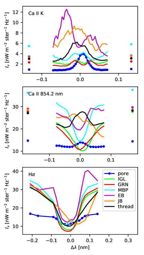
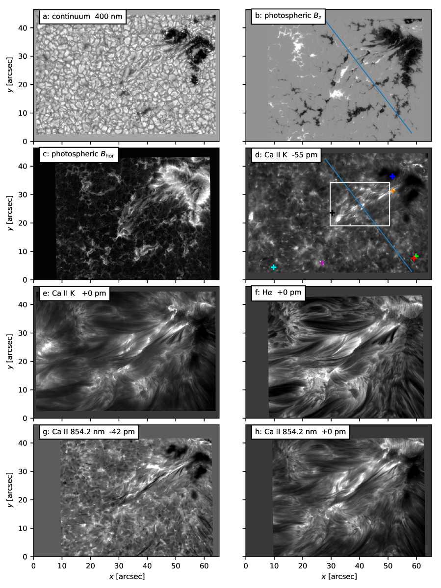
Figure 1 shows an overview of the observations. The CRISP and CHROMIS data do not have the same FOV, and the centers of their FOV are not exactly at the same location. Panel a shows the continuum, with a group of large pores in the upper right and smaller pores scattered throughout the FOV. Panels b and c show the photospheric magnetic field (see Sec. 2.3). The FOV shows a complex pattern of positive and negative magnetic flux density, with elongated granulation and extended patches of medium strength horizontal field indicating ongoing flux emergence along the line between arcsec and arcsec. The images in the wings of the Ca II lines (panels d and g) show enhanced brightness above the flux emergence. The line-core images (panels e, f, and h) show a complex structure of chromospheric fibrils, indicating the complex topology of the chromospheric magnetic field. We note that panels e and f show fan-shaped jets around arcsec. The accompanying movie of the entire time sequence display strong dynamics including fine bright threads seen in the blue wing of Ca II K (panel d).
Figure 2 shows example line profiles at the locations of the colored crosses in panel d of Fig. 1, and illustrates the wavelength sampling. The line profiles show a large variation depending on the sampled structure. Of particular interest are the Ca II K profiles in the Ellerman bomb, the location from where the jets are launched (jet base), and the bright thread. The profiles have a high intensity in their line cores, and the cores are very wide compared to the more usual profiles in a granule, intergranular lane and the magnetic bright point. We also note that that the magnetic bright point has the highest intensity in the outermost points at nm.
2.3 Further data products
The entire sequence of Fe I data was inverted with a modified version of the Milne-Eddington inversion code presented in Asensio Ramos & de la Cruz Rodríguez (2015) operating in 1.5D mode, yielding estimates of the magnetic field vector in the photosphere. Example images of the observations and the inferred photospheric magnetic field are shown in Fig. 1.
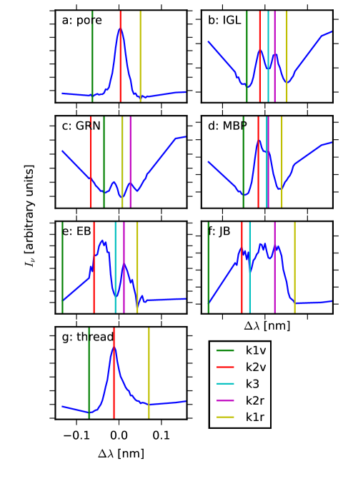
We used an automated feature detection code to characterize the Ca II K line profiles. This code tries to find the location of the K1v, K2v, K3, K2r, and K1r spectral features for a given line profile. Once it has found these locations it stores the intensity and wavelength of the features, and computes the full-width-at-half-maximum (FWHM) and full-width-at-quarter-maximum (FWQM) by finding the wavelengths of the two outmost intersections of the line profile between K1v and K1r with the line
| (1) |
where for the FWHM and for the FWQM. The difference of the two wavelengths is the width measure. The code also stores the average of these wavelengths, which measures the Doppler-shift of the emission peak at the quarter and half maximum. Not all profiles show a central emission core or a K3 minimum. Such profiles are flagged as pure absorption (no K1 and K2) or single-peaked (no K2r and K3). In Fig. 3 we show the results of the feature finder for the pixels indicated with plus-signs in Fig. 1. The code correctly fits the features in panels a, b, d, and g, but misidentifies one or more features in panels c and e. The profile in panel f show three emission peaks with some additional wiggles, and the classification using K2v, K3, K2r is too simple. We note that because of the limited sampling of the line profile (see Fig. 2) we cannot determine the location of all features accurately, such as the locations of K1v in panels e and f. Manual inspection of images of the various fitted properties show however that the misidentification rate is rather small, and typically happens for very bright and wide profiles with multiple emission peaks such as in panel e and f of Fig. 3.
3 Results
3.1 Ca II K brightness and chromospheric heating
The precise mechanisms that heat the solar chromosphere under various circumstances are not yet known and understood. These processes must act because the average chromosphere emits more radiation than predicted by radiative equilibrium models (e.g. Withbroe & Noyes 1977), even in the quiet Sun. A fundamental problem is that neither the local heating rate nor even the local radiative cooling rate can be measured directly. The local net radiative cooling rate is
| (2) |
with the extinction coefficient, the source function, and the intensity, all as function of frequency and direction . What we measure is the emergent intensity:
| (3) |
with a location sufficiently deep in the atmosphere so that the integrand is zero and the optical depth. The only way to get a quantitative estimate of the cooling rate from observations is to construct an atmosphere model that is consistent with the observed intensity and compute the radiative cooling in the model. This is beyond the scope fo the current paper.
Here we take a simpler approach: We assume that the Ca II K intensity, frequency-integrated over the inner wings and line core, correlates with the total radiative cooling along the line-of-sight, and thus with conversion of non-radiative and non-thermal energy into heat in order to sustain the radiative losses. This assumption is justified based on radiative transfer modelling that shows that increased Ca II K emission indeed corresponds to elevated temperatures in the chromosphere in both 1D semi-empirical atmosphere models as well as those computed from radiation-MHD models (Vernazza et al. 1981; Carlsson & Leenaarts 2012).
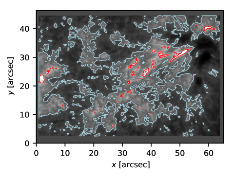
In order to make the connection between our spectrally-resolved data and total core emission we summed the intensities at all wavelength positions for each timestep in our Ca II K data. We then selected two brightness thresholds at and 2.09 times the spatially and temporally averaged value of the data. The lower threshold divides the images into rather persistent dark and intermediately-bright areas. Inside the intermediate-brightness bin we see many instances of high brightness, some persisting over the whole time series, and some more intermittent, which fall above the 2.09 level. The selection of the thresholds is somewhat arbitrary, but serves adequately to roughly separate the images into quiet-Sun-like areas, the flux-emergence area and smaller high-brightness events. We show this in Fig. 4 and the accompanying online movie.
In total, 66.8% of the pixels fall into the low-brightness bin, 32.6% in the intermediate bin and 0.60% in the high brightness bin. The high-brightness pixels produce 3.3% of the total integrated observed emission in the intermediate and high brightness bin (i.e., the area associated with the flux emergence). Inspection of the high-brightness bin events shows that they are typically associated to cancellation of opposite polarity field in the photosphere and/or reconnection between horizontal and vertical field in the low chromosphere. They are spectacular, but appear to play only a minor role in the overall heating because they cover only a small fraction of the area. The exact percentages obviously depend on the threshold values, as well as the selection of the FOV. In our case some of the areas around the edges of the FOV with intermediate brightness do not contain vigorous flux emergence. However, even with different threshold values and FOV selection the question of chromospheric heating is then: what caused the overwhelming majority of the emission in the emerging flux region?
3.2 Ca II K profile properties and total brightness
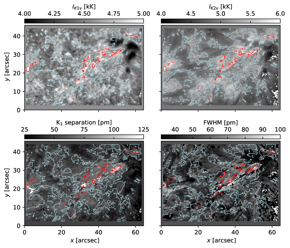
In Fig. 5 we show images of the intensity of K1v and K2v as well as the wavelength separation of the K1 minima and the FWHM of the central emission peaks. The pores show the lowest K1v intensity, with kK, and the highest intensities are in the bright patches associated with the flux emergence where can be as high as 5.78 kK. The K2v intensities are higher, between 4.02 kK and 7.04 kK, with again the lowest values in the pores, and the highest values in the region of the ongoing flux emergence. The K1 separation and FWHM roughly fall between 30 pm and 170 pm, with lower values for the FWHM. The lowest width values are associated with pores and areas with weak photospheric magnetic field (compare Fig. 1). The highest widths are located again where the flux emergence is taking place. The black pixels around this area are locations where the classification algorithm failed in correctly determining one or more of the spectral features.
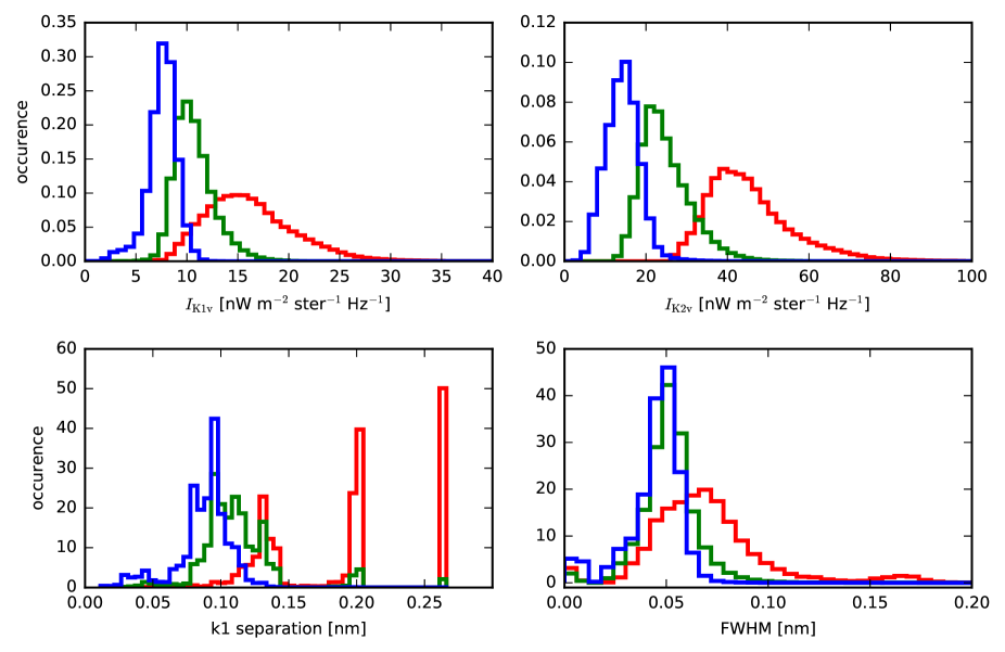
In Figure 6 we show histograms of the Ca II K profile properties separated for each brightness bin. These histograms were created from the entire time-series. The mean K1v and K2v brightness increases when going from the low-brightness to the high-brightness bin. The same holds for the K1 separation. We note that the peaks in the histogram at 0.20 nm and 0.26 nm are a consequence of the large wavelength difference between the densely sampled line core and the two outlying outer wavelength points. The peaks are formed of those pixels where one or both of the minima are located in the outer points. The FWHM of the central emission peak behaves differently: the distributions for the low and intermediate brightness bins are very similar, and only the high-brightness bin shows a clear increase in FWHM.
3.3 Ca II K intensity and chromospheric magnetic field
We now turn our attention to the relation between the summed Ca II K intensity and the chromospheric magnetic field. The datasets contain full-Stokes observations in the Ca II 854.2 nm line. The polarimetric accuracy of this data is of the order of and meaningful signal in Stokes and is only obtained in a small fraction of the pixels, mainly located close to the pores. The Stokes signals are stronger but also here we do not detect signal throughout the field-of-view. In order to boost the signal-to-noise ratio we therefore opted to compute the total linear polarization:
| (4) |
where the sum is taken over all 21 observed wavelength positions in the Ca II 854.2 nm line. Including the far wing wavelengths does not add photospheric contamination because the polarization signal there is very weak. We also computed the integrated circular polarization:
| (5) |
where the sum is over the observed wavelength positions less than 42.5 pm from nominal line center. The wavelength range is constrained to the line core because Stokes shows noticeable photospheric signal in the line wings.
These quantities do not provide quantitative information about the horizontal and vertical components of the magnetic field, but do provide qualitative information: Stronger TLP (TCP) generally means stronger horizontal (vertical) magnetic field strengths around the height where the response function peaks. This height is located roughly between in the 1D semi-empirical FALC atmosphere model (Quintero Noda et al. 2016). In this flux emergence region this optical depth might be lower owing to the elevated density compared to the quiet Sun (Quintero Noda et al. 2017).
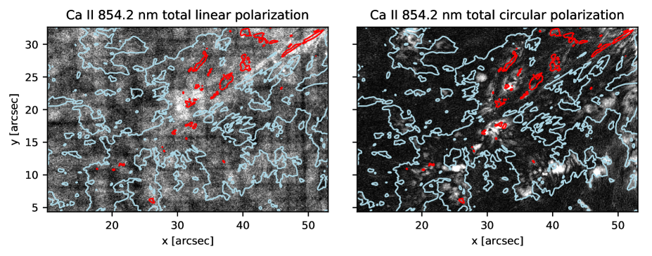
The upper row of Fig. 7 shows maps of TLP and TCP with wavelength-summed Ca II K brightness contours overplotted at 09:43:54 UT. This time was chosen to minimize the time difference between the Ca II K and Ca II 854.2 nm scans owing to the different cadence of the CRISP and CHROMIS observations.
The Ca II 854.2 nm line is not only sensitive to the Zeeman effect, but also to atomic level polarization due to anisotropy in the radiation field and depolarization by the Hanle effect (Manso Sainz & Trujillo Bueno 2010; Carlin & Asensio Ramos 2015; Štěpán & Trujillo Bueno 2016). Three-dimensional radiative transfer calculations computed with a 3D radiation-MHD simulation as input atmosphere indicate that atomic level polarization and the Hanle effect generate linear polarization signals at the level. These signals dominate in quiet Sun areas of the model atmosphere, while in areas with strong horizontal fields the linear polarization is dominated by the Zeeman effect (Štěpán & Trujillo Bueno 2016). This gives us reason to believe that our conclusions are not affected by scattering polarization.
The TLP map structure is also not caused by cross-talk from Stokes . While the TLP map shows a rough correlation with the wavelength-summed CaII 854.2 nm intensity, sharp individual bright and dark structures structures in the intensity image are not present in the TLP map, which would be the case if the cause was cross-talk.
The TLP panel shows a pattern of dark square grid lines. These are the edges of the MOMFBD image restoration patches. At the edges the final signal is composed of a linear combination of both patches, lowering the noise, and thus appearing dark in the image. The TLP appears concentrated within the blue contours, with the highest values in the upper-right corners close to the pores (cf. Fig. 4. While some of the highest TLP values fall within the red high-Ca II K-brightness contour, there are many high values that do not.
The TCP panel shows more intermittent structure, with the strongest signal above the photospheric magnetic elements. Almost all signal is contained within the blue contours.
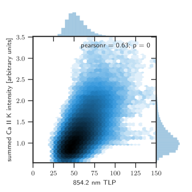
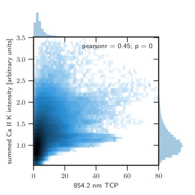
The lower panels show joint probability distributions of the total linear and circular polarization in the Ca II 854.2 nm line and the wavelength-summed Ca II K intensity. The TLP panel shows that high TLP correlates with high Ca II K brightness, even though the distribution has a fairly large spread. The TCP panel shows a more ambiguous result. The correlation coefficient is still relatively high at , but the shape of the distribution shows considerably more structure than the TLP panel. The most notable case is the horizontal arm at a Ca II K intensity of .
We interpret these results as follows: The flux emergence produces a multitude of low-lying magnetic field lines in the lower chromosphere. These field lines are rooted in photospheric magnetic elements. Above these elements the magnetic field still has an appreciable vertical component, which is depicted in the TCP image, but further away from the magnetic elements the field is mainly horizontal. The horizontal field in the low chromosphere where the TLP signal is formed appears space-filling. The correlation between TLP and Ca II K intensity implies a heating function that scales with magnetic field strength. Because neither diagnostics are linear (unknown dependence for Ca II K brightness and chromospheric heating, while TLP scales as ) we cannot comment on the functional dependence of heating as function of horizontal field strength.
3.4 Non-LTE Inversions
| Quantity | -image | -slice |
|---|---|---|
| -8.2 | -7.8 | |
| 0.6 | 0.4 | |
| 10 | 9 | |
| 9 | 5 | |
| none | 4 | |
| 2 | 3 | |
| inclination | 2 | 3 |
| azimuth | 1 | 1 |
As a final step in the analysis of the data we estimate the 3D structure of the temperature in the emerging flux region through non-Local Thermodynamic Equilibrium (non-LTE) inversion of our observations.
We perform the inversion using the STiC inversion code developed by de la Cruz Rodríguez et al. (2016). This code uses the RH code (Uitenbroek 2001) as the radiative transfer engine. It assumes that each pixel is an independent plane-parallel atmosphere, includes the effect of partial redistribution (PRD) in moving atmospheres following Leenaarts et al. (2012), and can solve the non-LTE radiative transfer problem for multiple atomic species and lines simultaneously.
The inversion code produces as output for each pixel a 1D atmosphere (temperature, vertical velocity, magnetic field vector and optionally microturbulence) on a height scale. The inversion code assumes hydrostatic equilibrium and a smooth variation of each parameter between the nodes.
Here we used the Ca II K line, the Ca II 854.2 nm line, the Fe I 630.1 nm and 630.2 nm lines and the continuum at 400.0 nm simultaneously. We treated the Ca II atom in non-LTE with the H&K lines in PRD. The Fe I lines are treated assuming LTE. We inverted the entire time series for all pixels along the blue line indicated in Fig. 1, as well as a 2D field-of-view (white rectangle in Fig. 1) in a single time step at 09:43:54 UT.
Owing to the different cadence of CHROMIS (14.5 s) and CRISP (36.6 s), the maximum time difference between different spectral line scans that are inverted together can be up to 18 s. For the time-dependent inversion this is an unavoidable limitation. The time step for which we invert a 2D patch was chosen so that the time difference between the observation of the central wavelength of Ca II K and Ca II 854.2 nm was 0.9 s, to minimise the inconsistencies of the multi-line inversion caused by the possibly fast temporal evolution in the chromosphere.
The -image and the -slice inversion were performed with slightly different setups, which are summarized in Table. 1.
The non-LTE inversion technique is a powerful method to derive atmospheric quantities. However, it has a number of limitations: The inversion assumes that each pixel is a plane-parallel atmosphere. Three-dimensional radiative transfer is however important in the cores of the Ca II lines (Leenaarts & Carlsson 2009; Leenaarts et al. 2009; Björgen et al. 2017), and its neglect might lead to errors in the upper chromosphere of the inferred atmosphere models.
The strongly scattering nature of these lines lead to a decreased contrast in the retrieved temperature maps. Test inversions with the Ca II 854.2 nm line indicate that small pockets of material cooler than 4000 K will typically not be retrieved (de la Cruz Rodríguez et al. 2012).
The inversions that we performed here assume a smooth variation of atmospheric parameters through spline interpolation in between the nodes (Ruiz Cobo & del Toro Iniesta 1992). While nodes can in principle be placed arbitrarily close together in -space, in practice placing them equidistantly is the most practical approach when inverting large numbers of pixels. Our results can therefore never represent sharp vertical gradients in, for example, magnetic field strength and temperature that we expect to be present in the solar atmosphere.
There is also a degeneracy between fitting line widths with microturbulence or temperature (cf. Figs. 4 and 5 of Carlsson et al. 2015, for an example in the Mg II h&k lines, which have a similar formation mechanism as the Ca II H&Klines.). In test computations we find that the latter effect can lead to temperature differences up to 1000 K in the inferred atmospheres when performing inversions with and without microturbulence.
Finally, the CRISP and CHROMIS data have different spatial resolution, and each wavelength position is observed at a different time, so that the spectrum fed into STiC is not strictly cotemporal, but can, in this case have a time difference up to 16 s between wavelength positions, which will affect results obtained for structures that evolve faster than that in time.
Despite these caveats, inversion of chromospheric lines is an excellent tool to build a spatially and temporally resolved picture of the solar atmosphere. It is a powerful method including much of the relevant physics, and is unbiased by human judgement.
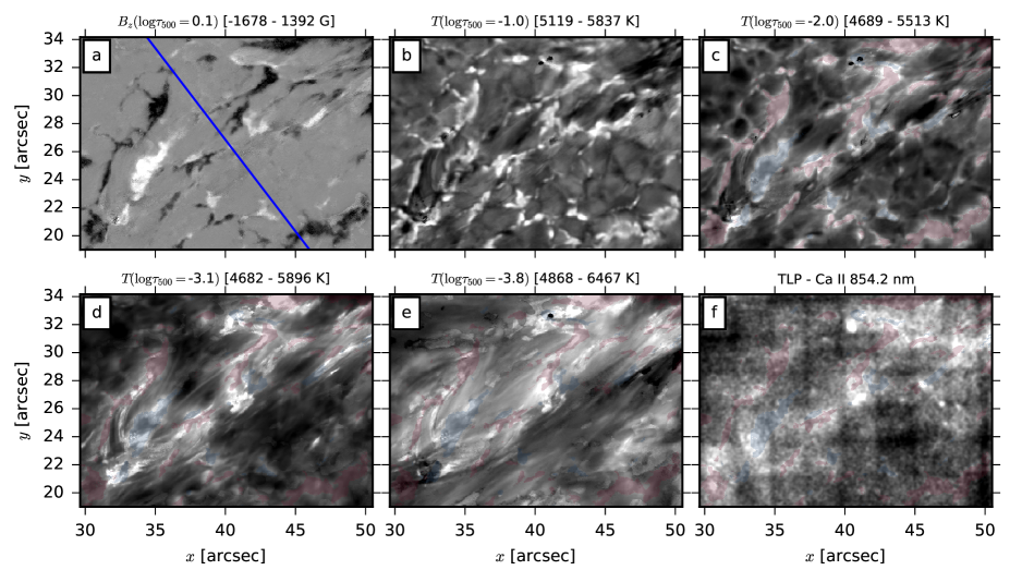
Figure 8 shows the results for the inversion of the 2D field-of-view. The most vigourous flux emergence is occurring in a diagonal band from arcsec to arcsec. It shows the spatial structure of the temperature at different heights in the atmosphere, together with the photospheric vertical magnetic field for context. At we see granulation and the heating in the magnetic elements. At we see some reversed granulation, and the heating of the magnetic elements is more extended owing to the fanning out of the magnetic field.
At the scene changes qualitatively. Strong increases in temperature start to appear that are not located on top of the photospheric field concentrations. In addition, a number of thin, thread-like regions of increased temperature are present that span between regions of opposite photospheric magnetic field polarity. At the temperature increase becomes space-filling in the emerging flux region, with typical temperatures around 6 kK. This behaviour is consistent with the usual picture of expansion of the magnetic field with height to form a magnetic canopy.
Above the inversion result is dominated by systematic errors and a lack of sensitivity, and therefore we do not show it here. Instead we show the cospatial Ca II 854.2 nm TLP map in panel f. Even though it is noisy, it shows a clear correlation with the in panel e.
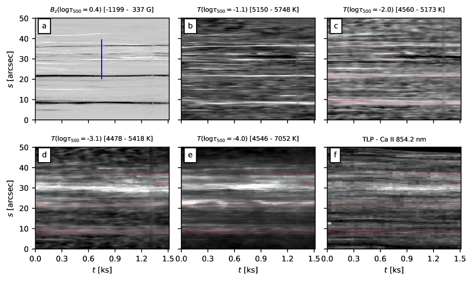
In Figure 9 we display the time variation of the inferred atmosphere along a cut through the emerging flux region. The location of this cut is indicated by the blue line in Fig. 1; the figure format is otherwise the same as for Fig. 8. We see a rather similar behaviour: at the photospheric flux concentrations appear bright; higher in the atmosphere the heating becomes more spread out, and is not co-spatial with the photospheric flux elements. Around the heating in the emerging flux region is rather homogenous, and the sites with the highest temperatures are mainly located between the photospheric flux elements. There is relatively little time variation in the temperature, indicating heating processes that are rather persistent in time.
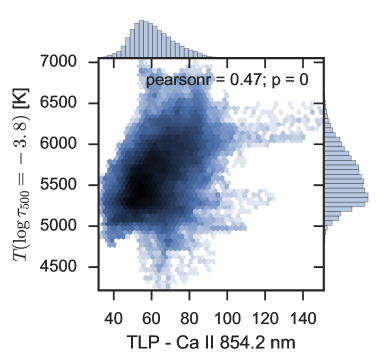
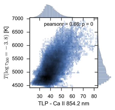
Finally, in Fig. 10 we show the correlation between the inferred gas temperature at and the total linear polarization in the Ca II 854.2 nm line. Both distributions have some outlying arms owing to noise and artefacts. but the bulk of the distributions follows a clear correlation, which is corroborated by the correlation coefficients.
4 Summary and Conclusions
We present imaging spectropolarimetric observations of active region NOAA 12593. The chromosphere above the flux emergence sites as seen in wavelength-summed Ca II K intensity is persistently brighter than the surrounding atmosphere where no flux emergence is taking place.
We divide the excess brightening into a spatially diffuse, persistent-in-time, intermediate brightness part and a spatially localized and more intermittent high-brightness part. The intermediate brightness bin is the dominant contributor to the overall brightness of the flux emergence region. We show that the excess brightness in the intermediate bin is caused by increased K1 (forming around the temperature minimum) and K2 (forming in the low chromosphere) intensity, as well as an increase in the K1 separation compared to the low-brightness bin, but the FWHM of the emission peak is not increased. This indicates that the excess heating in the chromosphere occurs already deep in the chromosphere, around the temperature minimum and just above it. The lack of increase in FWHM might indicate that the upper chromosphere is not as strongly affected by the heating. Alternatively, the Ca II K FWHM might just not be sufficiently sensitive to temperature. It would be interesting to repeat this analysis with Mg II h&k data taken with the Interface Region Imaging Spectrograph (IRIS, De Pontieu et al. 2014), because those lines have higher opacity and are sensitive to temperatures at somewhat larger heights.
Analysis of the total linear polarization of the Ca II 854.2 nm line reveals that the emerging flux region is likely permeated with space-filling horizontal magnetic fields. The TLP correlates strongly with the wavelength-summed Ca II K intensity, much more so than the TCP, which traces vertical field in the chromosphere. This result indicates that the chromospheric heating rate increases with increasing horizontal field strength.
Our multi-line, multi-atom, non-LTE inversions confirm that the excess brightening observed in Ca II K indeed corresponds to an increased temperature at the temperature minimum and above. The inverted image shows instances of thin threads of increased temperature around . We conjecture that these are the signature of heating by current sheets as seen in numerical simulations. (Galsgaard et al. 2005; Hansteen et al. 2015). In our observations the threads appear around the height of the temperature minimum. This might be caused by a strong overlying canopy of previously emerged magnetic field that forces the interaction region where the currents form to lower heights than in the simulations.
Around the temperature in the flux emergence region appears more homogenous, both in space and time, even though structuring is still visible. We speculate that this more homogenous heating can be caused by heating through ion-neutral collisions, which appear to give rise to a more homogenous distribution of currents and temperature than Spitzer-resistivity only (Arber et al. 2007; Leake & Linton 2013). We note, however, that systematic biases intrinsic to our inversions might influence the temperature structure on which we base our conclusions.
In this paper we present a global analysis of the heating in the chromosphere of emerging flux regions using multi-line observations at high spatial and temporal resolution. Future work should focus in detail on individual heating events, such as the bright thread-like regions of increased temperature that we find in the inversions, as well as a more detailed analysis of the spatial and temporal structure of the temperature in the solar chromosphere.
Our spectropolarimetric observations in the Ca II 854.2 nm line have too-low signal to noise ( to derive the horizontal magnetic field in the chromosphere. This highlights the need for imaging-spectropolarimetry in chromospheric lines with a sensitivity at least an order of magnitude better, so that inversion codes can provide estimates of the magnetic field vector at multiple heights in the chromosphere.
Acknowledgements.
The Swedish 1-m Solar Telescope is operated by the Institute for Solar Physics of Stockholm University in the Spanish Observatorio del Roque de los Muchachos of the Instituto de Astrofísica de Canarias. Computations were performed on resources provided by the Swedish National Infrastructure for Computing (SNIC) at the PDC Centre for High Performance Computing (PDC-HPC) at the Royal Institute of Technology in Stockholm as well at the High Performance Computing Center North (HPC2N). This research was supported by the CHROMOBS and CHROMATIC grants of the Knut och Alice Wallenberg foundation. JdlCR is supported by grants from the Swedish Research Council (2015-03994), the Swedish National Space Board (128/15). SD and JdlCR are financially supported by the Swedish Civil Contingencies Agency (MSB). MC has received support from the Research Council of Norway.References
- Arber et al. (2007) Arber, T. D., Haynes, M., & Leake, J. E. 2007, ApJ, 666, 541
- Asensio Ramos & de la Cruz Rodríguez (2015) Asensio Ramos, A. & de la Cruz Rodríguez, J. 2015, A&A, 577, A140
- Athay (1975) Athay, R. G., ed. 1975, The Solar Chromosphere and Corona: Quiet Sun
- Björgen et al. (2017) Björgen, J. P., Sukhorukov, A. V., Leenaarts, J., et al. 2017, A&A, submitted
- Carlin & Asensio Ramos (2015) Carlin, E. S. & Asensio Ramos, A. 2015, ApJ, 801, 16
- Carlsson & Leenaarts (2012) Carlsson, M. & Leenaarts, J. 2012, A&A, 539, A39
- Carlsson et al. (2015) Carlsson, M., Leenaarts, J., & De Pontieu, B. 2015, ApJ, 809, L30
- Carlsson et al. (1992) Carlsson, M., Rutten, R. J., & Shchukina, N. G. 1992, A&A, 253, 567
- Cheung & Isobe (2014) Cheung, M. C. M. & Isobe, H. 2014, Living Reviews in Solar Physics, 11, 3
- Cheung et al. (2010) Cheung, M. C. M., Rempel, M., Title, A. M., & Schüssler, M. 2010, ApJ, 720, 233
- Danilovic (2017) Danilovic, S. 2017, A&A, 601, A122
- de la Cruz Rodríguez et al. (2015a) de la Cruz Rodríguez, J., Hansteen, V., Bellot-Rubio, L., & Ortiz, A. 2015a, ApJ, 810, 145
- de la Cruz Rodríguez et al. (2016) de la Cruz Rodríguez, J., Leenaarts, J., & Asensio Ramos, A. 2016, ApJ, 830, L30
- de la Cruz Rodríguez et al. (2015b) de la Cruz Rodríguez, J., Löfdahl, M. G., Sütterlin, P., Hillberg, T., & Rouppe van der Voort, L. 2015b, A&A, 573, A40
- de la Cruz Rodríguez et al. (2012) de la Cruz Rodríguez, J., Socas-Navarro, H., Carlsson, M., & Leenaarts, J. 2012, A&A, 543, A34
- De Pontieu et al. (2014) De Pontieu, B., Title, A. M., Lemen, J. R., et al. 2014, Sol. Phys., 289, 2733
- Edvardsson et al. (1993) Edvardsson, B., Andersen, J., Gustafsson, B., et al. 1993, A&A, 275, 101
- Galsgaard et al. (2005) Galsgaard, K., Moreno-Insertis, F., Archontis, V., & Hood, A. 2005, ApJ, 618, L153
- Hansteen et al. (2015) Hansteen, V., Guerreiro, N., De Pontieu, B., & Carlsson, M. 2015, ApJ, 811, 106
- Hansteen et al. (2017) Hansteen, V. H., Archontis, V., Pereira, T. M. D., et al. 2017, ApJ, 839, 22
- Holweger & Mueller (1974) Holweger, H. & Mueller, E. A. 1974, Sol. Phys., 39, 19
- Khomenko & Collados (2012) Khomenko, E. & Collados, M. 2012, ApJ, 747, 87
- Leake & Arber (2006) Leake, J. E. & Arber, T. D. 2006, A&A, 450, 805
- Leake & Linton (2013) Leake, J. E. & Linton, M. G. 2013, ApJ, 764, 54
- Leenaarts & Carlsson (2009) Leenaarts, J. & Carlsson, M. 2009, in Astronomical Society of the Pacific Conference Series, Vol. 415, The Second Hinode Science Meeting: Beyond Discovery-Toward Understanding, ed. B. Lites, M. Cheung, T. Magara, J. Mariska, & K. Reeves, 87
- Leenaarts et al. (2009) Leenaarts, J., Carlsson, M., Hansteen, V., & Rouppe van der Voort, L. 2009, ApJ, 694, L128
- Leenaarts et al. (2012) Leenaarts, J., Pereira, T., & Uitenbroek, H. 2012, A&A, 543, A109
- Manso Sainz & Trujillo Bueno (2010) Manso Sainz, R. & Trujillo Bueno, J. 2010, ApJ, 722, 1416
- Martínez-Sykora et al. (2017) Martínez-Sykora, J., De Pontieu, B., Carlsson, M., et al. 2017, ArXiv e-prints [arXiv:1708.06781]
- Martínez-Sykora et al. (2012) Martínez-Sykora, J., De Pontieu, B., & Hansteen, V. 2012, ApJ, 753, 161
- Martínez-Sykora et al. (2015) Martínez-Sykora, J., De Pontieu, B., Hansteen, V., & Carlsson, M. 2015, Philosophical Transactions of the Royal Society of London Series A, 373, 20140268
- Martínez-Sykora et al. (2008) Martínez-Sykora, J., Hansteen, V., & Carlsson, M. 2008, ApJ, 679, 871
- Martínez-Sykora et al. (2009) Martínez-Sykora, J., Hansteen, V., & Carlsson, M. 2009, ApJ, 702, 129
- Neckel & Labs (1984) Neckel, H. & Labs, D. 1984, Sol. Phys., 90, 205
- Ortiz et al. (2014) Ortiz, A., Bellot Rubio, L. R., Hansteen, V. H., de la Cruz Rodríguez, J., & Rouppe van der Voort, L. 2014, ApJ, 781, 126
- Ortiz et al. (2016) Ortiz, A., Hansteen, V. H., Bellot Rubio, L. R., et al. 2016, ApJ, 825, 93
- Peter et al. (2014) Peter, H., Tian, H., Curdt, W., et al. 2014, Science, 346, 1255726
- Quintero Noda et al. (2017) Quintero Noda, C., Kato, Y., Katsukawa, Y., et al. 2017, MNRAS, 472, 727
- Quintero Noda et al. (2016) Quintero Noda, C., Shimizu, T., de la Cruz Rodríguez, J., et al. 2016, MNRAS, 459, 3363
- Ruiz Cobo & del Toro Iniesta (1992) Ruiz Cobo, B. & del Toro Iniesta, J. C. 1992, ApJ, 398, 375
- Scharmer (2017) Scharmer, G. 2017, in preparation
- Scharmer et al. (2003) Scharmer, G. B., Bjelksjo, K., Korhonen, T. K., Lindberg, B., & Petterson, B. 2003, in Society of Photo-Optical Instrumentation Engineers (SPIE) Conference Series, Vol. 4853, Innovative Telescopes and Instrumentation for Solar Astrophysics, ed. S. L. Keil & S. V. Avakyan, 341–350
- Scharmer et al. (2008) Scharmer, G. B., Narayan, G., Hillberg, T., et al. 2008, ApJ, 689, L69
- Schmieder et al. (2014) Schmieder, B., Archontis, V., & Pariat, E. 2014, Space Sci. Rev., 186, 227
- Schrijver et al. (1989) Schrijver, C. J., Cote, J., Zwaan, C., & Saar, S. H. 1989, ApJ, 337, 964
- Shelyag et al. (2016) Shelyag, S., Khomenko, E., de Vicente, A., & Przybylski, D. 2016, ApJ, 819, L11
- Skumanich et al. (1975) Skumanich, A., Smythe, C., & Frazier, E. N. 1975, ApJ, 200, 747
- Toriumi et al. (2017) Toriumi, S., Katsukawa, Y., & Cheung, M. C. M. 2017, ApJ, 836, 63
- Tortosa-Andreu & Moreno-Insertis (2009) Tortosa-Andreu, A. & Moreno-Insertis, F. 2009, A&A, 507, 949
- Uitenbroek (2001) Uitenbroek, H. 2001, ApJ, 557, 389
- Štěpán & Trujillo Bueno (2016) Štěpán, J. & Trujillo Bueno, J. 2016, ApJ, 826, L10
- van Noort et al. (2005) van Noort, M., Rouppe van der Voort, L., & Löfdahl, M. G. 2005, Sol. Phys., 228, 191
- Vernazza et al. (1981) Vernazza, J. E., Avrett, E. H., & Loeser, R. 1981, ApJS, 45, 635
- Withbroe & Noyes (1977) Withbroe, G. L. & Noyes, R. W. 1977, ARA&A, 15, 363