Hadronic light-by-light scattering amplitudes from lattice QCD
versus dispersive sum rules

Abstract

The hadronic contribution to the eight forward amplitudes of light-by-light scattering ($\gamma^{*}\gamma^{*}\to\gamma^{*}\gamma^{*}$) is computed in lattice QCD. Via dispersive sum rules, the amplitudes are compared to a model of the $\gamma^{*}\gamma^{*}\to{\rm hadrons}$ cross sections in which the fusion process is described by hadronic resonances. Our results thus provide an important test for the model estimates of hadronic light-by-light scattering in the anomalous magnetic moment of the muon, $a_{\mu}^{\rm HLbL}$. Using simple parametrizations of the resonance $M\to\gamma^{*}\gamma^{*}$ transition form factors, we determine the corresponding monopole and dipole masses by performing a global fit to all eight amplitudes. Together with a previous dedicated calculation of the $\pi^{0}\to\gamma^{*}\gamma^{*}$ transition form factor, our calculation provides valuable information for phenomenological estimates of $a_{\mu}^{\rm HLbL}$. The presented calculations are performed in two-flavor QCD with pion masses extending down to 190 MeV at two different lattice spacings. In addition to the fully connected Wick contractions, on two lattice ensembles we also compute the (2+2) disconnected class of diagrams, and find that their overall size is compatible with a parameter-free, large-$N$ inspired prediction, where $N$ is the number of colors. Motivated by this observation, we estimate in the same way the disconnected contribution to $a_{\mu}^{\rm HLbL}$.

I Introduction

The non-vanishing probability of two photons scattering off each other is a striking prediction of quantum electrodynamics (QED) Heisenberg1936 ; Karplus:1951uo . The smallness of the cross section has so far prohibited a direct experimental observation, although evidence for the phenomenon has recently been found by the ATLAS experiment in relativistic heavy-ion collisions Aaboud:2017bwk . Equally interesting is the scattering of spacelike virtual photons, $\gamma^{*}\gamma^{*}\to\gamma^{*}\gamma^{*}$. While the contributions of virtual leptons are calculable in QED perturbatively, the hadronic contributions require a nonperturbative approach. When the photons are real or spacelike, dispersive sum rules can be used to express the forward $\gamma^{*}\gamma^{*}$ scattering amplitudes in terms of experimentally more accessible $\gamma^{*}\gamma^{*}$-fusion cross sections Pascalutsa:2010sj ; Pascalutsa:2012pr ; Danilkin:2016hnh ; Dai:2017cvz . The hadronic contributions to the $\gamma^{*}\gamma^{*}\to\gamma^{*}\gamma^{*}$ amplitudes can also be computed ab initio using lattice QCD Green:2015sra .

One very timely application of hadronic light-by-light (HLbL) scattering is the anomalous magnetic moment of the muon, $a_{\mu}=\frac{1}{2}(g-2)_{\mu}$. The current discrepancy between the direct measurement of $a_{\mu}$ and the Standard Model prediction amounts to about 3.6 standard deviations Blum:2013xva . While the current theory and experimental errors are comparable in size, two new $(g-2)_{\mu}$ experiments Venanzoni:2014ixa ; Otani:2015lra in preparation at Fermilab and J-PARC aim at reducing the experimental error by a factor of four. The largest sources of theory error are contributions from the hadronic vacuum polarization (HVP) and from HLbL scattering. The latter is expected to dominate in the future in view of the dedicated measurements at $e^{+}e^{-}$ colliders ever better constraining the former. Although an active area of research, the experimental data needed for the recently proposed data-driven dispersive approaches to HLBL Colangelo:2014dfa ; Colangelo:2014pva ; Colangelo:2015ama ; Pauk:2014rfa ; Hagelstein:2017obr are harder to obtain, and lattice QCD calculations are in particularly high demand.

Lattice QCD calculations of hadron structure have been steadily advancing in recent years. Several collaborations calculate hadronic observables directly at physical values of the quark masses. At least two collaborations are addressing the HLbL contribution to $(g-2)_{\mu}$ on the lattice Blum:2014oka ; Blum:2015gfa ; Blum:2016lnc ; Green:2015sra ; Green:2015mva ; Asmussen:2016lse ; Asmussen:2017bup . Although the calculation poses serious challenges due to the complexity of the four-point function and the long-range nature of the dominant contribution, as a spacelike quantity it is well suited for a first-principles treatment directly in the Euclidean theory. A second role of lattice QCD is to provide the necessary hadronic input for the model and dispersive approaches to $a_{\mu}^{\rm HLbL}$. Model calculations (see e.g. Nyffeler:2017ohp for a recent overview) consistently suggest that the contribution of the pseudoscalar mesons ($\pi^{0},\eta,\eta^{\prime}$) is dominant, and therefore determining their respective transition form factors is of primary importance. A first calculation of the $\pi^{0}\to\gamma^{*}\gamma^{*}$ transition form factor in the range of photon virtualities relevant to $(g-2)_{\mu}$ has been carried out on the lattice Gerardin:2016cqj . An extension of this calculation to the $\eta,\eta^{\prime}$ mesons is possible, though more demanding, due to the appearance of disconnected Wick-contraction diagrams. Computing the spectrum and two-photon coupling of the scalar, axial-vector and tensor mesons is qualitatively more complicated in lattice QCD, since these states are resonances and require a dedicated treatment.

In many ways, the light-by-light scattering amplitudes are the more accessible observable in lattice calculations, because they involve spacelike photons that can be treated directly in the Euclidean theory. The lattice calculation of the cross section $\gamma^{*}\gamma^{*}\to\pi\pi$ is for instance more complex than calculating the cross section $\gamma^{*}\gamma^{*}\to\gamma^{*}\gamma^{*}$ for spacelike photons. In experiments, the weakness of the electromagnetic coupling would make such a measurement impractical, but in lattice QCD the factor $e^{4}$ merely multiplies a four-point correlation function at the end of the calculation.

In this article, we compute the HLbL scattering amplitude for spacelike photons in lattice QCD. Being parametrized by functions of six Lorentz invariants, it is a complicated object. We focus on the forward amplitudes because they are simpler functions of three invariants and, using the optical theorem, they are related to $\gamma^{*}\gamma^{*}\to\,{\rm hadrons}$ cross sections. Our objectives are:

• Provide a stringent test that the light-by-light amplitude for spacelike photons is correctly described by the type of hadronic model used so far to estimate $a_{\mu}^{\rm HLbL}$. The model includes the exchange of pseudoscalar, scalar, axial-vector and tensor mesons.

• Provide information on their two-photon transition form factors via global fits.

• Compare the transition form factors to phenomenological determinations based on light-by-light sum rules.

In Green:2015sra , we laid out the method and computed the forward amplitude sensitive to the total transverse $\gamma^{*}\gamma^{*}$ cross section, ${\cal M}_{\rm TT}$, via a dispersive sum rule. Here we extend the comparison between lattice data and phenomenological parametrizations of the $\gamma^{*}\gamma^{*}\to\,{\rm hadrons}$ cross sections to encompass all eight forward amplitudes. This more extensive analysis allows us to place much stronger constraints on the size of the contributions of different resonances, because they contribute to different amplitudes with different weight factors, often even with opposite signs.

Our lattice calculation is performed in QCD with two flavors of light quarks; it involves pion masses down to 190 MeV and two lattice spacings. While a fully realistic lattice calculation would have to include at least a dynamical strange quark, the present calculation does provide a suitable test of hadronic models via dispersive sum rules, since at the required level of precision it is fairly straightforward to adapt these models to QCD without the strange quark, as discussed in section V.

Here we have computed the fully connected and the dominant disconnected Wick-contraction diagrams. We discuss what these classes of diagrams correspond to in terms of the quantum numbers of the exchanged resonances. The large-$N$ inspired approximation that a quark loop containing a single, vector-current insertion gives a negligible contribution, corresponds, in two-flavor QCD, to including only isovector resonances, enhanced by a factor of 34/9. This interpretation of the fully connected class of diagrams was first pointed out in Bijnens:2015jqa ; Bijnens:2016hgx , mainly concerning the pseudoscalar sector; see also the arguments presented in Jin:2016rmu . We rederive the result in detail in the SU(2) and in the SU(3) flavor symmetric theory under slightly weaker assumptions; see section III.2.

The paper is organized as follows. We begin by introducing the theoretical background for light-by-light scattering in section II. We then describe the lattice method for computing the hadronic light-by-light amplitude, including the analytic continuation and the numerical method to obtain the fully connected and the (2+2) disconnected four-point function (section III). Section IV presents our numerical results in two-flavor QCD, while some additional material is provided in appendix B. After introducing the details of the hadronic model for the $\gamma^{*}\gamma^{*}\to\,{\rm hadrons}$ cross sections in section V and appendix A, we perform fits to the lattice data in section VI. We compare the results for the transition form factors to existing phenomenological estimates. In section VII, we discuss our results on the leading disconnected diagrams to the HLbL amplitude and present what results would have to be obtained in lattice QCD for the connected and the leading disconnected diagram contributions to $a_{\mu}^{\rm HLbL}$ in order to confirm the state-of-the-art model estimate. We conclude in section VIII.

II Forward light-by-light scattering and sum rules

In order to establish our notation, we start by recalling the dispersive sum rules for the scattering of spacelike photons Pascalutsa:2010sj ; Pascalutsa:2012pr . Just as for real photons Gerasimov:1973ja , they are based on unitarity and analyticity of the forward scattering amplitude. More specifically, the optical theorem allows one to relate the absorptive part of the $\gamma^{\ast}(\lambda_{1},q_{1})\gamma^{\ast}(\lambda_{2},q_{2})\to\gamma^{\ast}(\lambda_{1}^{\prime},q_{1})\gamma^{\ast}(\lambda_{2}^{\prime},q_{2})$ forward scattering amplitude to fusion cross sections for the process $\gamma^{\ast}\gamma^{\ast}\to\mathrm{X}$, where X stands for any $C$-parity even final state. The relevant kinematic variables are the photon virtualities, $q_{i}^{2}=-Q_{i}^{2}$, ($i=1,2$), and the crossing-symmetric variable $\nu=q_{1}\cdot q_{2}$, which is related to the squared center-of-mass energy by $s=2\nu-Q_{1}^{2}-Q_{2}^{2}$. Denoting the absorptive part of the helicity amplitude $\mathcal{M}_{\lambda^{\prime}_{1}\lambda^{\prime}_{2},\lambda_{1}\lambda_{2}}$ by

$$W_{\lambda^{\prime}_{1}\lambda^{\prime}_{2},\lambda_{1}\lambda_{2}}=\mathrm{Im}\left(\mathcal{M}_{\lambda^{\prime}_{1}\lambda^{\prime}_{2},\lambda_{1}\lambda_{2}}\right)\,,$$ (1)

the optical theorem yields (with a factor of one half because both photons are identical, and $\mathrm{d}\Gamma_{\mathrm{X}}$ is the phase space for a final state X)

$$W_{\lambda^{\prime}_{1}\lambda^{\prime}_{2},\lambda_{1}\lambda_{2}}=\frac{1}{2}\int\mathrm{d}\Gamma_{X}\ (2\pi)^{4}\delta^{4}(q_{1}+q_{2}-p_{\mathrm{X}})\,{\cal M}_{\lambda_{1}\lambda_{2}}(q_{1},q_{2};p_{\mathrm{X}})\,{\cal M}^{\ast}_{\lambda^{\prime}_{1}\lambda^{\prime}_{2}}(q_{1},q_{2};p_{\mathrm{X}})\,,$$ (2)

where ${\cal M}_{\lambda_{1}\lambda_{2}}(q_{1},q_{2};p_{\mathrm{X}})$ denotes the invariant helicity amplitude for the fusion process

$$\gamma^{\ast}(\lambda_{1},q_{1})+\gamma^{\ast}(\lambda_{2},q_{2})\to\mathrm{X}(p_{\mathrm{X}})\,.$$ (3)

The helicity amplitudes are related to the Feynman amplitudes by

$$\mathcal{M}_{\lambda_{1}^{\prime}\lambda_{2}^{\prime}\lambda_{1}\lambda_{2}}(q_{1},q_{2})=\mathcal{M}_{\mu\nu\rho\sigma}(q_{1},q_{2})\ \epsilon^{*\mu}(\lambda_{1}^{\prime},q_{1})\ \epsilon^{*\nu}(\lambda_{2}^{\prime},q_{2})\ \epsilon^{\rho}(\lambda_{1},q_{1})\ \epsilon^{\sigma}(\lambda_{2},q_{2})\,.$$ (4)

Using parity and time-reversal invariance, we are left with only eight independent amplitudes $\mathcal{M}_{\lambda^{\prime}_{1}\lambda^{\prime}_{2},\lambda_{1}\lambda_{2}}$ Budnev:1971sz . Forming linear combinations, we can consider eight amplitudes which are either even (first six amplitudes) or odd (last two amplitudes) with respect to the variable $\nu$:

$$\mathcal{M}_{TT}=\frac{1}{2}(\mathcal{M}_{++,++}+\mathcal{M}_{+-,+-})\,,\ \mathcal{M}_{TT}^{\tau}=\mathcal{M}_{++,--}\,,\$$

$$\mathcal{M}_{TL}=\mathcal{M}_{+0,+0}\,,\ \mathcal{M}_{LT}={\cal M}_{0+,0+}\,,\ \mathcal{M}_{TL}^{\tau}=\frac{1}{2}(\mathcal{M}_{++,00}+\mathcal{M}_{0+,-0})\,,\ \mathcal{M}_{LL}=\mathcal{M}_{00,00}\,,$$

$$\mathcal{M}_{TT}^{a}=\frac{1}{2}(\mathcal{M}_{++,++}-\mathcal{M}_{+-,+-})\,,\ \mathcal{M}_{TL}^{a}=\frac{1}{2}(\mathcal{M}_{++,00}-\mathcal{M}_{0+,-0})\,.$$

In terms of the Feynman amplitudes, the eight independent helicity amplitudes are then given by Budnev:1971sz

$$\mathcal{M}_{TT} = \frac{1}{4}R^{\mu\mu^{\prime}}R^{\nu\nu^{\prime}}\mathcal{M}_{\mu^{\prime}\nu^{\prime}\mu\nu}\,,$$ (5a)

$$\mathcal{M}_{TT}^{\tau} = \frac{1}{4}\left[R^{\mu\nu}R^{\mu^{\prime}\nu^{\prime}}+R^{\mu\nu^{\prime}}R^{\mu^{\prime}\nu}-R^{\mu\mu^{\prime}}R^{\nu\nu^{\prime}}\right]\mathcal{M}_{\mu^{\prime}\nu^{\prime}\mu\nu}\,,$$ (5b)

$$\mathcal{M}_{TT}^{a} = \frac{1}{4}\left[R^{\mu\nu}R^{\mu^{\prime}\nu^{\prime}}-R^{\mu\nu^{\prime}}R^{\mu^{\prime}\nu}\right]\mathcal{M}_{\mu^{\prime}\nu^{\prime}\mu\nu}\,,$$ (5c)

$$\mathcal{M}_{TL} = \frac{1}{2}R^{\mu\mu^{\prime}}k_{2}^{\nu}k_{2}^{\nu^{\prime}}\mathcal{M}_{\mu^{\prime}\nu^{\prime}\mu\nu}\,,$$ (5d)

$$\mathcal{M}_{LT} = \frac{1}{2}k_{1}^{\mu}k_{1}^{\mu^{\prime}}R^{\nu\nu^{\prime}}\mathcal{M}_{\mu^{\prime}\nu^{\prime}\mu\nu}\,,$$ (5e)

$$\mathcal{M}_{LL} = k_{1}^{\mu}k_{1}^{\mu^{\prime}}k_{2}^{\nu}k_{2}^{\nu^{\prime}}\mathcal{M}_{\mu^{\prime}\nu^{\prime}\mu\nu}\,,$$ (5f)

$$\mathcal{M}_{TL}^{a} = -\frac{1}{8}\left[R^{\mu\nu}k_{1}^{\mu^{\prime}}k_{2}^{\nu^{\prime}}+R^{\mu\nu^{\prime}}k_{1}^{\mu^{\prime}}k_{2}^{\nu}+(\mu\nu\leftrightarrow\mu^{\prime}\nu^{\prime})\right]\mathcal{M}_{\mu^{\prime}\nu^{\prime}\mu\nu}\,,$$ (5g)

$$\mathcal{M}_{TL}^{\tau} = -\frac{1}{8}\left[R^{\mu\nu}k_{1}^{\mu^{\prime}}k_{2}^{\nu^{\prime}}-R^{\mu\nu^{\prime}}k_{1}^{\mu^{\prime}}k_{2}^{\nu}+(\mu\nu\leftrightarrow\mu^{\prime}\nu^{\prime})\right]\mathcal{M}_{\mu^{\prime}\nu^{\prime}\mu\nu}\,,$$ (5h)

where the projector $R^{\mu\nu}$ onto the subspace orthogonal to $q_{1}$ and $q_{2}$, and the vectors $k_{1}$ and $k_{2}$ are defined in Appendix A. The eight helicity amplitudes are functions of $(\nu,Q_{1}^{2},Q_{2}^{2})$. Then, for fixed photon virtualities $Q_{1}^{2}$ and $Q_{2}^{2}$, the sum rules can be generically written as Pascalutsa:2012pr

$$\mathcal{M}_{\rm even}(\nu) = \frac{2}{\pi}\int_{\nu_{0}}^{\infty}\!d\nu^{\prime}\frac{\nu^{\prime}}{\nu^{\prime\,2}-\nu^{2}-i\epsilon}W_{\rm even}(\nu^{\prime})\,,$$ (6a)

$$\mathcal{M}_{\rm odd}(\nu) = \frac{2\nu}{\pi}\int_{\nu_{0}}^{\infty}\!d\nu^{\prime}\frac{1}{\nu^{\prime\,2}-\nu^{2}-i\epsilon}W_{\rm odd}(\nu^{\prime})\,,$$ (6b)

assuming the convergence of the integral. Here $\nu_{0}\equiv\frac{1}{2}(Q_{1}^{2}+Q_{2}^{2})$. If the integral does not converge, it is necessary to introduce a subtraction

$$\mathcal{M}_{\rm even}(\nu) = \mathcal{M}_{\rm even}(0)+\frac{2\nu^{2}}{\pi}\int_{\nu_{0}}^{\infty}\!d\nu^{\prime}\frac{1}{\nu^{\prime}(\nu^{\prime\,2}-\nu^{2}-i\epsilon)}W_{\rm even}(\nu^{\prime})\,,$$ (7a)

$$\mathcal{M}_{\rm odd}(\nu) = \nu\mathcal{M}^{\prime}_{\rm odd}(0)+\frac{2\nu^{3}}{\pi}\int_{\nu_{0}}^{\infty}\!d\nu^{\prime}\frac{1}{\nu^{\prime 2}(\nu^{\prime\,2}-\nu^{2}-i\epsilon)}W_{\rm odd}(\nu^{\prime})\,.$$ (7b)

Finally, the absorptive parts $W_{\lambda^{\prime}_{1}\lambda^{\prime}_{2},\lambda_{1}\lambda_{2}}$ of those eight independent amplitudes, given by Eq. (2), are expressed in terms of the $\gamma^{\ast}\gamma^{\ast}\to\mathrm{X}$ fusion cross sections Budnev:1974de ,

$$W_{++,++}+W_{+-,+-} \equiv 2\sqrt{X}\,\left(\sigma_{0}+\sigma_{2}\right)=2\sqrt{X}\,\left(\sigma_{\parallel}+\sigma_{\perp}\right)\equiv 4\sqrt{X}\,\sigma_{TT}\,,$$ (8a)

$$W_{++,--} \equiv 2\sqrt{X}\,\left(\sigma_{\parallel}-\sigma_{\perp}\right)\equiv 2\sqrt{X}\,\tau_{TT}\,,$$ (8b)

$$W_{++,++}-W_{+-,+-} \equiv 2\sqrt{X}\,\left(\sigma_{0}-\sigma_{2}\right)\equiv 4\sqrt{X}\,\tau^{a}_{TT}\,,$$ (8c)

$$W_{+0,+0} \equiv 2\sqrt{X}\,\sigma_{TL}\,,$$ (8d)

$$W_{0+,0+} \equiv 2\sqrt{X}\,\sigma_{LT}\,,$$ (8e)

$$W_{++,00}+W_{0+,-0} \equiv 4\sqrt{X}\,\tau_{TL}\,,$$ (8f)

$$W_{++,00}-W_{0+,-0} \equiv 4\sqrt{X}\,\tau^{a}_{TL}\,,$$ (8g)

$$W_{00,00} \equiv 2\sqrt{X}\,\sigma_{LL}\,,$$ (8h)

where $X=\nu^{2}-Q_{1}^{2}Q_{2}^{2}$ is the virtual-photon flux factor. Here, $L$ and $T$ refer to longitudinal and transverse polarizations respectively. The cross sections $\sigma$ are positive, but the interference terms $\tau$ are not sign-definite. The relevant cross sections for resonance contributions in each channel are explicitly given in Appendix A in terms of transition form factors.

Thus, using Eqs. (6) and (8), we obtain the following dispersive sum rules, valid for fixed photon virtualities $Q_{1}^{2},Q_{2}^{2}>0$ Pascalutsa:2012pr :

$$\overline{\mathcal{M}}_{TT}=\frac{1}{2}\left(\overline{\mathcal{M}}_{++,++}(\nu)+\overline{\mathcal{M}}_{+-,+-}(\nu)\right) = \frac{4\nu^{2}}{\pi}\int_{\nu_{0}}^{\infty}\!\!d\nu^{\prime}\,\frac{\sqrt{X^{\prime}}\sigma_{TT}(\nu^{\prime})}{\nu^{\prime}(\nu^{\prime\,2}-\nu^{2}-i\epsilon)}\,,$$ (9a)

$$\overline{\mathcal{M}}_{TT}^{\tau}=\overline{\mathcal{M}}_{++,--}(\nu) = \frac{4\nu^{2}}{\pi}\int_{\nu_{0}}^{\infty}\!\!d\nu^{\prime}\,\frac{\sqrt{X^{\prime}}\tau_{TT}(\nu^{\prime})}{\nu^{\prime}(\nu^{\prime\,2}-\nu^{2}-i\epsilon)}\,,$$ (9b)

$$\overline{\mathcal{M}}_{TT}^{a}=\frac{1}{2}\left(\overline{\mathcal{M}}_{++,++}(\nu)-\overline{\mathcal{M}}_{+-,+-}(\nu)\right) = \frac{4\nu^{3}}{\pi}\int_{\nu_{0}}^{\infty}\!\!d\nu^{\prime}\,\frac{\sqrt{X^{\prime}}\,\tau_{TT}^{a}(\nu^{\prime})}{\nu^{\prime\,2}(\nu^{\prime\,2}-\nu^{2}-i\epsilon)}\,,$$ (9c)

$$\overline{\mathcal{M}}_{TL}=\overline{\mathcal{M}}_{+0,+0}(\nu) = \frac{4\nu^{2}}{\pi}\int_{\nu_{0}}^{\infty}\!\!d\nu^{\prime}\,\frac{\sqrt{X^{\prime}}\sigma_{TL}(\nu^{\prime})}{\nu^{\prime}(\nu^{\prime\,2}-\nu^{2}-i\epsilon)}\,,$$ (9d)

$$\overline{\mathcal{M}}_{LT}=\overline{\mathcal{M}}_{0+,0+}(\nu) = \frac{4\nu^{2}}{\pi}\int_{\nu_{0}}^{\infty}\!\!d\nu^{\prime}\,\frac{\sqrt{X^{\prime}}\sigma_{LT}(\nu^{\prime})}{\nu^{\prime}(\nu^{\prime\,2}-\nu^{2}-i\epsilon)}\,,$$ (9e)

$$\overline{\mathcal{M}}_{TL}^{\tau}=\frac{1}{2}\left(\overline{\mathcal{M}}_{++,00}(\nu)+\overline{\mathcal{M}}_{0+,-0}(\nu)\right) = \frac{4\nu^{2}}{\pi}\int_{\nu_{0}}^{\infty}\!\!d\nu^{\prime}\,\frac{\sqrt{X^{\prime}}\,\tau_{TL}(\nu^{\prime})}{\nu^{\prime}(\nu^{\prime\,2}-\nu^{2}-i\epsilon)}\,,$$ (9f)

$$\overline{\mathcal{M}}_{TL}^{a}=\frac{1}{2}\left(\overline{\mathcal{M}}_{++,00}(\nu)-\overline{\mathcal{M}}_{0+,-0}(\nu)\right) = \frac{4\nu^{3}}{\pi}\int_{\nu_{0}}^{\infty}\!\!d\nu^{\prime}\,\frac{\sqrt{X^{\prime}}\,\tau^{a}_{TL}(\nu^{\prime})}{\nu^{\prime\,2}(\nu^{\prime\,2}-\nu^{2}-i\epsilon)}\,,$$ (9g)

$$\overline{\mathcal{M}}_{LL}=\overline{\mathcal{M}}_{00,00}(\nu) = \frac{4\nu^{2}}{\pi}\int_{\nu_{0}}^{\infty}\!\!d\nu^{\prime}\,\frac{\sqrt{X^{\prime}}\,\sigma_{LL}(\nu^{\prime})}{\nu^{\prime}(\nu^{\prime\,2}-\nu^{2}-i\epsilon)}\,,$$ (9h)

where we use the notation $\overline{\mathcal{M}}(\nu)\equiv\mathcal{M}(\nu)-\mathcal{M}(0)$ or $\overline{\mathcal{M}}(\nu)\equiv\mathcal{M}(\nu)-\nu\mathcal{M}^{\prime}(0)$ respectively for the even and odd amplitudes. We always consider the subtracted sum rules, even when the unsubtracted version is well defined, since the subtraction has the effect of suppressing the high-energy contributions. Evaluating the sum rules using phenomenological inputs on the two-photon fusion processes, one can confront the results with the light-by-light forward amplitudes computed on the lattice. In section V, we will present an empirical model for the description of the two-photon fusion processes and subsequently, by comparing it with our lattice results, we will be able to extract information about the $\gamma^{*}\gamma^{*}\to M$ transition form factors. Before coming to that, we describe the lattice QCD approach to calculating HLBL scattering amplitudes in the following two sections.

III Lattice QCD and light-by-light scattering

III.1 The scattering amplitude in Euclidean field theory

The Feynman amplitudes can be obtained via the calculation of the following Euclidean four-point correlation function

$$\Pi^{E}_{\mu\nu\rho\sigma}(Q_{1},Q_{2})=\sum_{X_{1},X_{2},X_{3}}\,\langle J_{\mu}(X_{1})J_{\nu}(X_{2})J_{\rho}(X_{3})J_{\sigma}(0)\rangle_{E}\,e^{iQ_{1}(X_{1}-X_{3})}\ e^{iQ_{2}X_{2}}\,,$$ (10)

where $J_{\mu}(X)$ is the Euclidean electromagnetic vector current ($J_{0}=j_{0}$, $J_{k}=ij_{k}$) and $Q_{i}$ are the Euclidean four-momenta ($q_{i}^{0}=-iQ_{i}^{0}$, $\vec{q}_{i}=\vec{Q}_{i}$). Indeed, using the Lehmann-Symanzik-Zimmermann reduction formula in Minkowski spacetime, the relation of this Euclidean correlator to the Feynman forward amplitudes in Minkowski spacetime is Green:2015sra

$$\mathcal{M}_{\mu\nu\rho\sigma}(q_{1},q_{2})=e^{4}i^{n_{0}}\Pi^{E}_{\mu\nu\rho\sigma}(Q_{1},Q_{2})\,,$$ (11)

where $n_{0}$ is the number of temporal indices. Each of the eight helicity amplitudes can be written as

$$\mathcal{M}(q_{1}^{2},q_{2}^{2},\nu) =T^{\mu\nu\mu^{\prime}\nu^{\prime}}(q_{1},q_{2})\,\mathcal{M}_{\mu\nu\mu^{\prime}\nu^{\prime}}(q_{1},q_{2})$$ (12)

$$=e^{4}\,T^{E}_{\mu\nu\mu^{\prime}\nu^{\prime}}(Q_{1},Q_{2})\,\Pi^{E}_{\mu\nu\mu^{\prime}\nu^{\prime}}(Q_{1},Q_{2})\,,$$

for some Minkowski tensor $T$, defined above through Eq. (5), and some Euclidean tensor $T^{E}$ given by

$$T^{E}_{\mu\nu\mu^{\prime}\nu^{\prime}}(Q_{1},Q_{2})=i^{n_{0}}T^{\mu\nu\mu^{\prime}\nu^{\prime}}(q_{1},q_{2})\,.$$ (13)

Thus, we define

$$R^{E}_{\mu\nu}(Q_{1},Q_{2})=i^{n_{0}}R^{\mu\nu}(q_{1},q_{2})=\delta_{\mu\nu}-\frac{1}{X}\,\bigl{\{}(Q_{1}\cdot Q_{2})\left(Q_{1\mu}\,Q_{2\nu}+Q_{1\nu}\,Q_{2\mu}\right)-Q_{1}^{2}\,Q_{2\mu}\,Q_{2\nu}-Q_{2}^{2}\,Q_{1\mu}\,Q_{1\nu}\bigr{\}}\,.$$ (14)

The case of $k_{i}$ in Eq. (5) requires a bit more care, since their definitions contain $\sqrt{X}$ and in Euclidean space $X=(Q_{1}\cdot Q_{2})^{2}-Q_{1}^{2}Q_{2}^{2}\leq 0$. In the Minkowski center of mass frame, if $q_{1}=(q_{1}^{0},\vec{q})$ and $q_{2}=(q_{2}^{0},-\vec{q})$, then $X=(q_{1}^{0}+q_{2}^{0})^{2}\vec{q}^{\,2}$ and we can evaluate the ordinary positive square root. Performing the Wick rotation, $q_{i}^{0}\to-iQ_{i}^{0}$, we get $\sqrt{X}\to-i(Q_{1}^{0}+Q_{2}^{0})|\vec{q}|=-i\sqrt{-X}$. Therefore, in Eq. (5), we perform the following replacements to obtain the amplitudes in Euclidean space:

$$\mathcal{M}_{\mu^{\prime}\nu^{\prime},\mu\nu} \to e^{4}\Pi^{E}_{\mu^{\prime}\nu^{\prime},\mu\nu}(Q_{1},Q_{2})\,,$$ (15a)

$$R^{\mu\nu} \to R^{E}_{\mu\nu}\,,$$ (15b)

$$k_{1} \to K_{1}\equiv i\sqrt{\frac{Q_{1}^{2}}{-X}}\left(Q_{2}-\frac{Q_{1}\cdot Q_{2}}{Q_{1}^{2}}Q_{1}\right)\,,$$ (15c)

$$k_{2} \to K_{2}\equiv i\sqrt{\frac{Q_{2}^{2}}{-X}}\left(Q_{1}-\frac{Q_{1}\cdot Q_{2}}{Q_{2}^{2}}Q_{2}\right)\,.$$ (15d)

These satisfy $K_{i}^{2}=-1$, $K_{i}\cdot Q_{i}=0$, $R^{E}_{\mu\nu}Q_{i\nu}=0$, $R^{E}_{\mu\alpha}R^{E}_{\alpha\nu}=R^{E}_{\mu\nu}$ and $R^{E}_{\mu\mu}=2$.

The largest value of $|\nu|$ that can be reached with Euclidean kinematics is limited by the virtualities of the photons, $|\nu|\leq(Q_{1}^{2}Q_{2}^{2})^{1/2}\leq\frac{1}{2}(Q_{1}^{2}+Q_{2}^{2})\equiv\nu_{0}$, while the nearest singularity is the s-channel $\pi^{0}$ pole located at $\nu_{\pi}=\frac{1}{2}(m_{\pi}^{2}+Q_{1}^{2}+Q_{2}^{2})$.

III.1.1 Special case of (anti)parallel momenta

The tensors $T^{E}$, resulting from Eq. (5) translated to Euclidean space using Eq. (15), are not defined for collinear $Q_{1}$ and $Q_{2}$, since in that case $X=0$. However, if we start with non-collinear momenta and rotate $Q_{2}$ toward being (anti)parallel with $Q_{1}$, then each tensor has such a limit. This limit depends on the initial direction of $Q_{2}$; we will use the average over this direction to define $T^{E}$ in the collinear limit.

We define the projector

$$\overline{R}_{\mu\nu}=\delta_{\mu\nu}-\frac{Q_{1\mu}Q_{1\nu}}{Q_{1}^{2}}\,,$$ (16)

and find that $R^{E}_{\mu\nu}\to\overline{R}_{\mu\nu}-V_{\mu}V_{\nu}$. Here $V$ is a unit vector orthogonal to $Q_{1}$, pointing in the direction from which $Q_{2}$ approached being collinear with $Q_{1}$. Since $K_{2}\cdot Q_{1}=i\sqrt{-X/Q_{2}^{2}}\to 0$, in the collinear limit any contraction of $T^{E}_{\mu\nu\mu^{\prime}\nu^{\prime}}$ with $Q_{1}$ will vanish. Thus, after averaging over all $V$ orthogonal to $Q_{1}$, each $T^{E}_{\mu\nu\mu^{\prime}\nu^{\prime}}$ will be a linear combination of

$$\overline{R}_{\mu\mu^{\prime}}\overline{R}_{\nu\nu^{\prime}}\,,\quad\overline{R}_{\mu\nu}\overline{R}_{\mu^{\prime}\nu^{\prime}}\,,\quad\overline{R}_{\mu\nu^{\prime}}\overline{R}_{\mu^{\prime}\nu}\,.$$ (17)

We obtain the prefactors by contracting the indices in three different ways. For this, we will make use of

$$K_{1}\cdot K_{2}=\frac{Q_{1}\cdot Q_{2}}{\sqrt{Q_{1}^{2}Q_{2}^{2}}}\to s\equiv\begin{cases}1&Q_{1},Q_{2}\text{ parallel}\\ -1&Q_{1},Q_{2}\text{ antiparallel}\end{cases}\,.$$ (18)

Denoting by $\langle\dots\rangle_{V}$ the average over $V$, we find

$$\langle R^{E}_{\mu\mu^{\prime}}R^{E}_{\nu\nu^{\prime}}\rangle_{V} =\frac{2}{5}\overline{R}_{\mu\mu^{\prime}}\overline{R}_{\nu\nu^{\prime}}+\frac{1}{15}\left(\overline{R}_{\mu\nu}\overline{R}_{\mu^{\prime}\nu^{\prime}}+\overline{R}_{\mu\nu^{\prime}}\overline{R}_{\mu^{\prime}\nu}\right)\,,$$ (19a)

$$\langle R^{E}_{\mu\mu^{\prime}}K_{2\nu}K_{2\nu^{\prime}}\rangle_{V} =\frac{-4}{15}\overline{R}_{\mu\mu^{\prime}}\overline{R}_{\nu\nu^{\prime}}+\frac{1}{15}\left(\overline{R}_{\mu\nu}\overline{R}_{\mu^{\prime}\nu^{\prime}}+\overline{R}_{\mu\nu^{\prime}}\overline{R}_{\mu^{\prime}\nu}\right)$$ (19b)

$$=\langle K_{1\mu}K_{1\mu^{\prime}}R^{E}_{\nu\nu^{\prime}}\rangle_{V}\,,$$ (19c)

$$\langle K_{1\mu}K_{1\mu^{\prime}}K_{2\nu}K_{2\nu^{\prime}}\rangle_{V} =\frac{1}{15}\left(\overline{R}_{\mu\mu^{\prime}}\overline{R}_{\nu\nu^{\prime}}+\overline{R}_{\mu\nu}\overline{R}_{\mu^{\prime}\nu^{\prime}}+\overline{R}_{\mu\nu^{\prime}}\overline{R}_{\mu^{\prime}\nu}\right)\,,$$ (19d)

$$\langle R^{E}_{\mu\mu^{\prime}}K_{1\nu}K_{2\nu^{\prime}}\rangle_{V} =-s\,\langle R^{E}_{\mu\mu^{\prime}}K_{2\nu}K_{2\nu^{\prime}}\rangle_{V}\,.$$ (19e)

III.2 Flavor structure of the four-point function

In numerical lattice QCD calculations of $n$-point functions, the quark path integral is evaluated analytically to yield a sum of contractions of quark propagators. For the four-point function of vector currents, these fall into five distinct topologies, illustrated in Fig. 1.

Figure 1: The five classes of quark contractions for four-point functions. In this work, we compute the leftmost, fully-connected set of contractions, as well as the (2+2) class of diagrams (second from the left).

The calculation of all Wick-contraction topologies is demanding. In many instances, disconnected diagram contributions have been found to make numerically small contributions to hadronic matrix elements, though not always Gulpers:2013uca . Quark loops generated by a single vector current have been empirically found to be particularly suppressed (see for instance Green:2015wqa ; Blum:2015you ; Gerardin:2016cqj ; DellaMorte:2017dyu ). At short distances, perturbation theory provides an explanation for the suppression of this type of contribution, since it requires the exchange of at least three gluons Chetyrkin:1994js . On the other hand, it is well known that the disconnected diagram is responsible for the difference between the pion and the $\eta^{\prime}$ mass in the pseudoscalar two-point function, and is therefore crucial at long distances.

The importance of the disconnected diagrams in the HLbL amplitude has been pointed out in Bijnens:2015jqa ; Bijnens:2016hgx , showing that the pion and $\eta^{\prime}$ pole contributions would have the wrong weight factors if only the connected diagrams were included. Here,

1. we use (a) flavor symmetry, either SU(2) or SU(3), and (b) the assumption that Wick-contraction diagrams where a vector current appears as the only insertion in a quark loop, thus producing a factor ${\rm Tr}\{\gamma_{\mu}S(X,X)\}$, are negligible;

2. we then derive the weight factors of non-singlet and singlet mesons in the fully connected and the (2+2) disconnected contribution to the HLbL amplitude;

3. we show that whenever the HLbL amplitude is dominated by the pole-exchange of an isovector resonance, isospin symmetry induces relations between different Wick-diagram topologies.

The main result is that under the assumptions stated under (1.), in the fully connected diagrams the non-singlet meson poles over-contribute by a factor $34/9$ (respectively a factor 3) in QCD with two (respectively three) degenerate flavors of quarks, while the singlet mesons do not contribute. The (2+2) disconnected diagrams contain the singlet-meson contribution and correct the fully connected diagram by compensating with $(-25/9)$ (respectively $-2$) times the non-singlet meson contribution. For QCD with a realistic quark spectrum, we expect the relations between the classes of diagrams to lie between the quoted predictions.

The starting point is the observation, based on Fig. 1, that the Wick contractions contributing to the HLbL amplitude can be written as (we drop the space-time arguments and indices of the four-point amplitudes)

$$\Pi^{\rm HLbL} = \sum_{f}{\cal Q}_{f}^{4}\Pi^{4}_{f}+\sum_{f_{1},f_{2}}{\cal Q}_{f_{1}}^{2}{\cal Q}_{f_{2}}^{2}\Pi_{f_{1},f_{2}}^{2+2}+\sum_{f_{1},f_{2}}{\cal Q}_{f_{1}}^{3}{\cal Q}_{f_{2}}\Pi_{f_{1},f_{2}}^{3+1}$$

$$+\sum_{f_{1},f_{2},f_{3}}{\cal Q}_{f_{1}}^{2}{\cal Q}_{f_{2}}{\cal Q}_{f_{3}}\Pi^{2+1+1}_{f_{1},f_{2},f_{3}}+\sum_{f_{1},f_{2},f_{3},f_{4}}{\cal Q}_{f_{1}}{\cal Q}_{f_{2}}{\cal Q}_{f_{3}}{\cal Q}_{f_{4}}\Pi^{1+1+1+1}_{f_{1},f_{2},f_{3},f_{4}}.$$

In the case that the quark masses are all equal, one can drop the flavor indices, e.g. $\Pi_{f_{1},f_{2}}^{2+2}\to\Pi^{2+2}$. In particular, let $\Pi$ be the four-point function of the ‘up’ current $\bar{u}\gamma_{\mu}u$. Since in that case $\sum_{f}{\cal Q}_{f}^{n}=1$ $\forall n$, and because all quark lines carry the same quark mass, the $\Pi^{X}_{f}$ are precisely the Wick contractions appearing in $\Pi$ ($X=4,\leavevmode\nobreak\ 2+2,\leavevmode\nobreak\ 3+1,\leavevmode\nobreak\ 2+1+1,\leavevmode\nobreak\ 1+1+1+1$), including the normalization. On the other hand, the HLbL amplitude is expressed as Wick contractions $\Pi^{X}_{f}$ weighted by polynomials in the quark charges.

An important observation is that with two flavors of quarks, there are only three linearly independent symmetric polynomials in ${\cal Q}_{u}$ and ${\cal Q}_{d}$, for instance

$$({\cal Q}_{u}^{4}+{\cal Q}_{d}^{4}),\qquad 2{\cal Q}_{u}^{2}{\cal Q}_{d}^{2},\qquad{\cal Q}_{u}{\cal Q}_{d}({\cal Q}_{u}^{2}+{\cal Q}_{d}^{2}).$$ (21)

With three flavors, there are four such independent polynomials in $({\cal Q}_{u},{\cal Q}_{d},{\cal Q}_{s})$, for instance

$$\begin{array}[]{ll}P_{1}\equiv({\cal Q}_{u}^{4}+{\cal Q}_{d}^{4}+{\cal Q}_{s}^{4}),&P_{2}\equiv({\cal Q}_{u}^{2}+{\cal Q}_{d}^{2}+{\cal Q}_{s}^{2})^{2},\phantom{\bigg{|}}\\ P_{3}\equiv({\cal Q}_{u}^{3}+{\cal Q}_{d}^{3}+{\cal Q}_{s}^{3})({\cal Q}_{u}+{\cal Q}_{d}+{\cal Q}_{s}),&P_{4}\equiv({\cal Q}_{u}^{2}+{\cal Q}_{d}^{2}+{\cal Q}_{s}^{2})({\cal Q}_{u}+{\cal Q}_{d}+{\cal Q}_{s})^{2},\end{array}$$ (22)

while $P_{5}\equiv({\cal Q}_{u}+{\cal Q}_{d}+{\cal Q}_{s})^{4}=6P_{1}-3P_{2}-8P_{3}+6P_{4}$.

III.2.1 The case of $N_{f}=2$ QCD

We assume exact isospin SU(2) symmetry. The photon couples to the electromagnetic current, whose isospin decomposition reads

$$J_{\mu}^{\rm e.m.}=J^{1}_{\mu}+J^{0}_{\mu},\qquad J^{1}_{\mu}=\frac{{\cal Q}_{u}-{\cal Q}_{d}}{2}(\bar{u}\gamma_{\mu}u-\bar{d}\gamma_{\mu}d),\qquad J^{0}_{\mu}=\frac{{\cal Q}_{u}+{\cal Q}_{d}}{2}(\bar{u}\gamma_{\mu}u+\bar{d}\gamma_{\mu}d).$$ (23)

The upper index on the current indicates the isospin quantum number $I=0,1$.

There are both isoscalar and isovector resonances that couple to two photons. As is well known, the coupling of an isovector resonance occurs only when one of the photons couples via the isoscalar part, and one couples via the isovector part of the e.m. current. Since the amplitude for a neutral pion to couple to two photons vanishes if either both are isoscalar (${\cal Q}_{u}={\cal Q}_{d}$) or both are isovector (${\cal Q}_{u}=-{\cal Q}_{d}$), and the coupling must be quadratic in the charges, it must be proportional to $({\cal Q}_{u}^{2}-{\cal Q}_{d}^{2})$. Then the contributions to $\Pi$ and $\Pi^{\rm HLbL}$ of an isovector resonance $M_{1}$ are related by

$$\Pi^{{\rm HLbL},M_{1}}=({\cal Q}_{u}^{2}-{\cal Q}_{d}^{2})^{2}\;\Pi^{M_{1}}.$$ (24)

Correspondingly, the dependence of the transition form factor of an isoscalar resonance on the quark charges is such that it contains two independent terms,

$${F}_{M^{0}\gamma^{*}\gamma^{*}}=({\cal Q}_{u}^{2}+{\cal Q}_{d}^{2}){\cal F}_{C}+({\cal Q}_{u}+{\cal Q}_{d})^{2}{\cal F}_{D}.$$ (25)

The notation indicates that ${\cal F}_{D}$ contains all the diagrams where at least one vector current appears isolated in a quark loop. In view of the form (25) of the $M^{0}\gamma\gamma$ vertex, the pole contribution of an isoscalar meson has the dependence

$$\Pi^{\rm HLbL,M^{0}}=({\cal Q}_{u}^{2}+{\cal Q}_{d}^{2})^{2}\Pi_{A}+({\cal Q}_{u}+{\cal Q}_{d})^{2}({\cal Q}_{u}^{2}+{\cal Q}_{d}^{2})\Pi_{B}+({\cal Q}_{u}+{\cal Q}_{d})^{4}\Pi_{C}.$$ (26)

on the quark charges, where the contributions $\Pi_{B}$ and $\Pi_{C}$ are only non-vanishing if the disconnected diagrams involving at least one isolated vector current inserted in a quark loop are non-vanishing. As discussed below, $\Pi_{B}$ is O($1/N$) and $\Pi_{C}$ is O($1/N^{2}$) in the large-$N$ power counting.

By identifying the polynomials in ${\cal Q}_{u}$ and ${\cal Q}_{d}$ in Eqs. (24) and (III.2), we obtain three conditions that relate the contributions of an isovector resonance to the various Wick contractions:

$$\Pi^{M^{1}} = \Pi^{4,M^{1}}+\Pi^{2+2,M^{1}}+\Pi^{3+1,M^{1}}+\Pi^{2+1+1,M^{1}}+\Pi^{1+1+1+1,M^{1}},$$ (27)

$$-\Pi^{M^{1}} = \Pi^{2+2,M^{1}}+\Pi^{2+1+1,M^{1}}+3\,\Pi^{1+1+1+1,M^{1}},$$ (28)

$$0 = \Pi^{3+1,M^{1}}+2\,\Pi^{2+1+1,M^{1}}+4\,\Pi^{1+1+1+1,M^{1}}.$$ (29)

Thus if for a specific kinematic regime one isovector resonance exchange dominates the HLbL amplitude, it is sufficient to compute three of the five Wick-contraction classes. For instance, $\Pi^{1+1+1+1,M^{1}}$ and $\Pi^{2+1+1,M^{1}}$ can be expressed in terms of the classes $\Pi^{4,M^{1}},\leavevmode\nobreak\ \Pi^{2+2,M^{1}}$ and $\Pi^{3+1,M^{1}}$ of diagrams. We also note the exact expression

$$\Pi^{4,M^{1}} = 2(\Pi^{M^{1}}+\Pi^{2+1+1,M^{1}}+3\Pi^{1+1+1+1,M^{1}}),$$ (30)

for the fully connected class of diagrams.

Similarly, equating the expressions (26) and (III.2) yields the relations

$$\Pi^{M^{0}}=\Pi_{A}+\Pi_{B}+\Pi_{C} = \Pi^{4,M^{0}}+\Pi^{2+2,M^{0}}+\Pi^{3+1,M^{0}}+\Pi^{2+1+1,M^{0}}+\Pi^{1+1+1+1,M^{0}},$$ (31)

$$\Pi_{A}+\Pi_{B}+3\Pi_{C} = \Pi^{2+2,M^{0}}+\Pi^{2+1+1,M^{0}}+3\,\Pi^{1+1+1+1,M^{0}},$$ (32)

$$2\Pi_{B}+4\Pi_{C} = \Pi^{3+1,M^{0}}+2\,\Pi^{2+1+1,M^{0}}+4\,\Pi^{1+1+1+1,M^{0}}.$$ (33)

Eliminating $\Pi^{2+2,M^{0}}$ and $\Pi^{3+1,M^{0}}$, we get

$$\Pi^{4,M^{0}}=2(-\Pi_{B}-3\Pi_{C}+\Pi^{2+1+1,M^{0}}+3\Pi^{1+1+1+1,M^{0}}).$$ (34)

III.2.2 Large-$N$ expectations

In terms of large-$N$ counting, where $N$ is the number of colors, every additional disconnected quark loop costs a factor $1/N$. However it is worth looking more closely how this property emerges. For instance, just keeping the leading class of diagrams $\Pi^{4,M}$ would not reproduce the correct dependence on ${\cal Q}_{u}$ and ${\cal Q}_{d}$ for the exchange of a single meson, be it isoscalar or isovector. Put in a different way, the relations (30) and (34) derived from isospin symmetry relate contributions to diagrams that scale differently with $N$.

The resolution of this apparent contradiction is that, at large $N$, neutral mesons are expected to come in degenerate pairs, one isoscalar, one isovector, due to the vanishing of the quark annihilation diagrams. Only when the sum of the contributions of a pair is considered, the large-$N$ counting should apply. Here we only apply the large-$N$ counting rule to the insertion of a vector current. Considering the sum of the contributions of such a pair, we obtain from (30–34) the relation

$$\Pi^{4,M^{0}+M^{1}} = 2\Big{(}\Pi^{M^{1}}-\Pi_{B}-3\Pi_{C}+\Pi^{2+1+1,M^{0}+M^{1}}+3\Pi^{1+1+1+1,M^{0}+M^{1}}\Big{)}.\qquad$$ (35)

Large-$N$ counting should apply at this point, and we expect to be able to neglect in first approximation $\Pi_{B},\Pi_{C}$ (down by $1/N$ and $1/N^{2}$ respectively) and the terms $\Pi^{2+1+1,M^{0}+M^{1}}$ and $\Pi^{1+1+1+1,M^{0}+M^{1}}$, since they are expected to be down by $1/N^{2}$ and $1/N^{3}$ respectively relative to $\Pi^{4,M^{0}+M^{1}}$. All neglected terms contain at least one isolated vector current in a quark loop. In that approximation, the leading diagram classes are given by

$$\Pi^{4,M^{0}+M^{1}} \approx 2\Pi^{M^{1}},$$ (36)

$$\Pi^{2+2,M^{0}+M^{1}} \approx -\Pi^{M^{1}}+\Pi^{M^{0}}.$$ (37)

Thus, using Eqs (36) and (24) we obtain for the fully connected contribution in Eq. (III.2)

$$({\cal Q}_{u}^{4}+{\cal Q}_{d}^{4})\Pi^{4,M^{0}+M^{1}}\approx({\cal Q}_{u}^{4}+{\cal Q}_{d}^{4})2\Pi^{M^{1}}=\frac{{\cal Q}_{u}^{4}+{\cal Q}_{d}^{4}}{({\cal Q}_{u}^{2}-{\cal Q}_{d}^{2})^{2}}2\Pi^{{\rm HLbL},M^{1}}=\frac{34}{9}\Pi^{{\rm HLbL},M^{1}},$$ (38)

where we have included the physical charges of the $u$ and $d$ quarks in the last step. The (2+2) disconnected diagrams complement the connected diagrams to yield the full contribution,

$$({\cal Q}_{u}^{2}+{\cal Q}_{d}^{2})^{2}\Pi^{2+2,M^{0}+M^{1}}\approx-\frac{25}{9}\Pi^{{\rm HLbL},M^{1}}+\Pi^{{\rm HLbL},M^{0}}.$$ (39)

The charge factors in Eqs. (38) and (39) agree with Refs. Bijnens:2015jqa ; Bijnens:2016hgx .

The stronger large-$N$ prediction, which however turns out not to be a good approximation in QCD, is that isoscalar and isovector states in each symmetry channel (pseudoscalars, scalars, tensors, etc.) compensate each other in the (2+2) disconnected diagrams, making the latter $1/N$ suppressed as compared to the fully connected diagrams. The channel where the degeneracy expected at large $N$ is most badly broken is the pseudoscalar channel, since $m_{\eta^{\prime}}\gg m_{\pi^{0}}$. Therefore, we expect the $\Pi^{2+2}$ class of diagrams to be dominated by the $\pi^{0}$ and $\eta^{\prime}$ contributions, since their contributions cancel each other to a far lesser extent than for other meson pairs such as $a_{2}$ and $f_{2}$. For instance, the empirical ratio of the two-photon widths of $a_{2}$ and $f_{2}$ are roughly as expected if one neglects disconnected diagrams (see Table 2 for the source of the phenomenological values),

$$\frac{\Gamma_{f_{2}\gamma\gamma}}{\Gamma_{a_{2}\gamma\gamma}}\approx\frac{(2.93\pm 0.40){\rm keV}}{(1.00\pm 0.06){\rm keV}}=2.93\pm 0.44\approx\frac{({\cal Q}_{u}^{2}+{\cal Q}_{d}^{2})^{2}}{({\cal Q}_{u}^{2}-{\cal Q}_{d}^{2})^{2}}=\frac{25}{9}\approx 2.7778.$$ (40)

On the other hand, using the phenomenological values Olive:2016xmw ; Larin:2010kq

$$\Gamma_{\eta^{\prime}\gamma\gamma}=4.35{\rm\,keV},\qquad\Gamma_{\pi^{0}\gamma\gamma}=7.82{\rm\,eV},$$ (41)

and the fact that $\Gamma\propto m_{P}^{3}|F_{P\gamma^{*}\gamma^{*}}(0,0)|^{2}$, we obtain

$$\frac{|{F}_{\eta^{\prime}\gamma^{*}\gamma^{*}}(0,0)|^{2}}{|{F}_{\pi^{0}\gamma^{*}\gamma^{*}}(0,0)|^{2}}\approx 1.56\neq\frac{({\cal Q}_{u}^{2}+{\cal Q}_{d}^{2})^{2}}{({\cal Q}_{u}^{2}-{\cal Q}_{d}^{2})^{2}}\approx 2.7778,$$ (42)

which does not agree well with the large-$N$ expectation and the approximation of $m_{\rm strange}=\infty$ implicitly made here by using relations derived in $N_{f}=2$ QCD. A further channel in which the large-$N$ expectations are not well fullfilled is the scalar sector; in particular, there does not seem to be an isovector analogue of the $f_{0}(600)$ meson. However, it turns out that the scalars make an overall small contribution to the light-by-light amplitudes.

III.2.3 The case of $N_{f}=3$ QCD

Here we assume exact SU(3) flavor symmetry, $m_{u}=m_{d}=m_{s}$. Since in the previous paragraphs we have treated the case of $N_{f}=2$ QCD, corresponding to $m_{s}=\infty$, one may hope that the real world lies somewhere in between these two idealized cases.

In nature, ${\cal Q}_{u}=2/3$ and ${\cal Q}_{d}={\cal Q}_{s}=-1/3$. Somewhat more generally, for ${\cal Q}_{u}+{\cal Q}_{d}+{\cal Q}_{s}=0$, the $SU(3)_{\rm f}$ decomposition reads

$$J_{\mu}^{\rm e.m.}=J^{3}_{\mu}+J^{8}_{\mu},\qquad J^{3}_{\mu}=\frac{{\cal Q}_{u}-{\cal Q}_{d}}{2}(\bar{u}\gamma_{\mu}u-\bar{d}\gamma_{\mu}d),\qquad J^{8}_{\mu}=\frac{{\cal Q}_{u}+{\cal Q}_{d}}{2}(\bar{u}\gamma_{\mu}u+\bar{d}\gamma_{\mu}d-2\bar{s}\gamma_{\mu}s).$$ (43)

It follows directly from ${\cal Q}_{u}+{\cal Q}_{d}+{\cal Q}_{s}=0$ that no diagrams with a single vector current inside a quark loop occurs in the HLbL amplitude: $\Pi^{3,1}$, $\Pi^{2+1+1}$ and $\Pi^{1+1+1+1}$ do not contribute. However it is useful to keep the charges generic to derive relations from flavor symmetry and large-$N$ arguments.

In the SU(3) symmetric theory, mesons come in octets and singlets. Taking the pseudoscalar sector as an example, the transition form factor of the neutral pion is given by $({\cal Q}_{u}^{2}-{\cal Q}_{d}^{2}){\cal F}_{8}$; neglecting again the single vector current inside a quark loop, the $\eta$ meson has the transition form factor $\sqrt{1/3}({\cal Q}_{u}^{2}+{\cal Q}_{d}^{2}-2{\cal Q}_{s}^{2}){\cal F}_{8}$. Under the same assumption, the form factor of the $\eta^{\prime}$ has a charge dependence given by $\sqrt{{2}/{3}}({\cal Q}_{u}^{2}+{\cal Q}_{d}^{2}+{\cal Q}_{s}^{2}){\cal F}_{0}$. Only in the strict large-$N$ limit would we have ${\cal F}_{0}={\cal F}_{8}$.

Thus the pole contribution of a meson octet to the four-point function of the electromagnetic current has the following dependence on the quark charges,

$$\Pi^{{\rm HLbL,oct}}=\frac{3}{4}\Big{[}({\cal Q}_{u}^{2}-{\cal Q}_{d}^{2})^{2}+\frac{1}{3}({\cal Q}_{u}^{2}+{\cal Q}_{d}^{2}-2{\cal Q}_{s}^{2})^{2}\Big{]}\Pi^{\rm oct},$$ (44)

where $\Pi^{\rm oct}$ is the octet contribution to $\Pi$. The corresponding expression for the singlet meson reads

$$\Pi^{{\rm HLbL,sgl}}=({\cal Q}_{u}^{2}+{\cal Q}_{d}^{2}+{\cal Q}_{s}^{2})^{2}\;\Pi^{\rm sgl}.$$ (45)

Matching the expressions (44) and (III.2), we obtain the relations

$$\frac{3}{2}\Pi^{\rm oct} = \Pi^{4,{\rm oct}},$$ (46)

$$-\frac{1}{2}\Pi^{\rm oct} = \Pi^{2+2,{\rm oct}}.$$ (47)

where we have consistently neglected the octet contribution to $\Pi^{3+1}$, $\Pi^{2+1+1}$ and $\Pi^{1+1+1+1}$. Under the corresponding assumption for the singlet contribution, we have

$$0 = \Pi^{4,{\rm sgl}},$$ (48)

$$\Pi^{\rm sgl} = \Pi^{2+2,{\rm sgl}}.$$ (49)

Combining these equations, we finally have the following expressions for the fully connected and the (2+2) disconnected class of diagrams,

$$({\cal Q}_{u}^{4}+{\cal Q}_{d}^{4}+{\cal Q}_{s}^{4})\Pi^{4,{\rm oct+sgl}} \approx P_{1}\;\Pi^{4,{\rm oct}}=P_{1}\cdot\frac{3}{2}\Pi^{{\rm oct}}=\frac{P_{1}}{P_{1}-\frac{1}{3}P_{2}}\Pi^{\rm HLbL,oct}$$ (50)

$$= 3\Pi^{\rm HLbL,oct},$$

$$({\cal Q}_{u}^{2}+{\cal Q}_{d}^{2}+{\cal Q}_{s}^{2})^{2}\Pi^{2+2,{\rm oct+sgl}} \approx -\frac{P_{2}}{3(P_{1}-\frac{1}{3}P_{2})}\Pi^{\rm HLbL,oct}+\Pi^{\rm HLbL,sgl}$$ (51)

$$= -2\Pi^{\rm HLbL,oct}+\Pi^{\rm HLbL,sgl}.$$

In the last of these equations we have set ${\cal Q}_{u}=2/3$, ${\cal Q}_{d}={\cal Q}_{s}=-1/3$.

III.3 Lattice calculation of the fully-connected vector four-point function

We now describe our method to calculate the six contractions that have fully connected quark lines (leftmost topology in Fig. 1), whereas the dominant class of disconnected diagrams (second diagram topology from the left in Fig. 1) is discussed in the next section.

We discretize the Euclidean four-point function using the local and conserved currents, as well as a contact operator,

$$J_{\mu}^{l}(X) =Z_{V}\bar{\psi}(X)\gamma_{\mu}\mathcal{Q}\psi(X),$$ (52a)

$$J_{\mu}^{c}(X) =\frac{1}{2}\left[\bar{\psi}(X+a\hat{\mu})(\gamma_{\mu}+1)U_{\mu}^{\dagger}(X)\mathcal{Q}\psi(X)+\bar{\psi}(X)(\gamma_{\mu}-1)U_{\mu}(X)\mathcal{Q}\psi(X+a\hat{\mu})\right],$$ (52b)

$$T_{\mu}(X) =\frac{1}{2}\left[\bar{\psi}(X+a\hat{\mu})(\gamma_{\mu}+1)U_{\mu}^{\dagger}(X)\mathcal{Q}\psi(X)-\bar{\psi}(X)(\gamma_{\mu}-1)U_{\mu}(X)\mathcal{Q}\psi(X+a\hat{\mu})\right],$$ (52c)

where $\psi=(u,d)^{T}$ is the doublet of light quarks, $\mathcal{Q}=\operatorname{diag}(\tfrac{2}{3},-\tfrac{1}{3})$ is the quark charge matrix, $U_{\mu}(X)$ are the gauge links, and $Z_{V}$ is the renormalization factor for the local current. We use one local and three conserved currents. In position space, the lattice four-point function is given by

$$\Pi^{\text{pos}}_{\mu_{1}\mu_{2}\mu_{3}\mu_{4}}(X_{1},X_{2},X_{3},0) =\Bigl{\langle}J_{\mu_{4}}^{l}(0)\Bigl{[}J_{\mu_{1}}^{c}(X_{1})J_{\mu_{2}}^{c}(X_{2})J_{\mu_{3}}^{c}(X_{3})+\delta_{\mu_{1}\mu_{2}}\delta_{X_{1}X_{2}}T_{\mu_{1}}(X_{1})J_{\mu_{3}}^{c}(X_{3})$$ (53)

$$\qquad+\delta_{\mu_{1}\mu_{3}}\delta_{X_{1}X_{3}}T_{\mu_{3}}(X_{3})J_{\mu_{2}}^{c}(X_{2})+\delta_{\mu_{2}\mu_{3}}\delta_{X_{2}X_{3}}T_{\mu_{3}}(X_{3})J_{\mu_{1}}^{c}(X_{1})$$

$$\qquad+\delta_{\mu_{1}\mu_{3}}\delta_{\mu_{2}\mu_{3}}\delta_{X_{1}X_{3}}\delta_{X_{2}X_{3}}J_{\mu_{3}}^{c}(X_{3})\Bigr{]}\Bigr{\rangle}\,.$$

The contact terms are present when two or three conserved currents coincide and serve to ensure that the conserved-current Ward identities hold. Using the backward lattice derivative $\Delta$, these take the form

$$\Delta_{\mu_{1}}^{X_{1}}\Pi^{\text{pos}}_{\mu_{1}\mu_{2}\mu_{3}\mu_{4}}=\Delta_{\mu_{2}}^{X_{2}}\Pi^{\text{pos}}_{\mu_{1}\mu_{2}\mu_{3}\mu_{4}}=\Delta_{\mu_{3}}^{X_{3}}\Pi^{\text{pos}}_{\mu_{1}\mu_{2}\mu_{3}\mu_{4}}=0\,.$$ (54)

In momentum space, we evaluate the Euclidean four-point function as

$$\Pi^{E}_{\mu\nu\rho\sigma}(Q_{1},Q_{2})=\sum_{X_{1},X_{2},X_{3}}e^{iQ_{1}(X_{1}+\tfrac{a}{2}\hat{\mu})}e^{iQ_{2}(X_{2}+\tfrac{a}{2}\hat{\nu})}e^{-iQ_{1}(X_{3}+\tfrac{a}{2}\hat{\rho})}\Pi^{\text{pos}}_{\mu\nu\rho\sigma}(X_{1},X_{2},X_{3},0)\,.$$ (55)

The fully-connected contribution to Eq. (55), which is the part proportional to ${\rm Tr\,}(\mathcal{Q}^{4})=\frac{17}{81}$, is evaluated using the method of sequential propagators. First, a point-source propagator

$$S_{0}(X)\equiv S(X,0),$$ (56)

where $S$ is the single-flavor all-to-all quark propagator (degenerate for $u$ and $d$), is computed from the origin. To concisely describe the sequential propagators, we introduce the “insertions” $\mathcal{J}_{\mu}(X)$ and $\mathcal{T}_{\mu}(X)$ for the conserved vector current and contact operator:

$$J_{\mu}^{c}(X) =\bar{\psi}\mathcal{J}_{\mu}(X)\mathcal{Q}\psi,$$ (57a)

$$T_{\mu}(X) =\bar{\psi}\mathcal{T}_{\mu}(X)\mathcal{Q}\psi.$$ (57b)

Formally, these objects have the same size as an all-to-all quark propagator, but they are exactly zero for all sites except those that are removed from $X$ by one lattice spacing. The point-source propagator is then combined with a plane wave and the conserved vector current insertion to form the source for new (sequential) propagators,

$$S_{Q,\mu}\equiv S\sum_{X}e^{-iQ(X+\tfrac{a}{2}\hat{\mu})}\mathcal{J}_{\mu}(X)S_{0}.$$ (58)

These, in turn, are used to form sources for double-sequential propagators

$$S_{Q_{1}\mu_{1};Q_{2}\mu_{2}} \equiv S\sum_{X}\left[e^{-iQ_{1}(X+\tfrac{a}{2}\hat{\mu}_{1})}\mathcal{J}_{\mu_{1}}(X)S_{Q_{2}\mu_{2}}+e^{-iQ_{2}(X+\tfrac{a}{2}\hat{\mu}_{2})}\mathcal{J}_{\mu_{2}}(X)S_{Q_{1}\mu_{1}}\right.$$ (59)

$$\left.+\,\delta_{\mu_{1}\mu_{2}}e^{-i(Q_{1}+Q_{2})(X+\tfrac{a}{2}\hat{\mu}_{1})}\mathcal{T}_{\mu_{1}}S_{0}\right].$$

Finally, noting that $\gamma_{5}\mathcal{J}_{\mu}(X)$ is anti-Hermitian and $\gamma_{5}\mathcal{T}_{\mu}(X)$ is Hermitian, the fully-connected four-point function is obtained as

$$\Pi^{E,\text{conn}}_{\mu\nu\rho\sigma}(Q_{1},Q_{2}) =-{\rm Tr\,}[\mathcal{Q}^{4}]Z_{V}\sum_{X_{2}}e^{iQ_{2}(X_{2}+\tfrac{a}{2}\hat{\nu})}\Bigl{\langle}{\rm Tr\,}\Bigl{(}\gamma_{\sigma}\gamma_{5}$$ (60)

$$\qquad\qquad\times\Bigl{[}S_{Q_{1}\mu;-Q_{1}\rho}^{\dagger}\gamma_{5}\mathcal{J}_{\nu}(X_{2})S_{0}+S_{0}^{\dagger}\gamma_{5}\mathcal{J}_{\nu}(X_{2})S_{-Q_{1}\mu;Q_{1}\rho}$$

$$\qquad\qquad\qquad-S^{\dagger}_{-Q_{1}\rho}\gamma_{5}\mathcal{J}_{\nu}(X_{2})S_{-Q_{1}\mu}-S^{\dagger}_{Q_{1}\mu}\gamma_{5}\mathcal{J}_{\nu}(X_{2})S_{Q_{1}\rho}$$

$$\qquad\qquad\qquad+\delta_{\mu\nu}e^{iQ_{1}(X_{2}+\tfrac{a}{2}\hat{\nu})}\bigl{(}S_{0}^{\dagger}\gamma_{5}\mathcal{T}_{\nu}(X_{2})S_{Q_{1}\rho}-S_{-Q_{1}\rho}^{\dagger}\gamma_{5}\mathcal{T}_{\nu}(X_{2})S_{0}\bigr{)}$$

$$\qquad\qquad\qquad+\delta_{\rho\nu}e^{-iQ_{1}(X_{2}+\tfrac{a}{2}\hat{\nu})}\bigl{(}S_{0}^{\dagger}\gamma_{5}\mathcal{T}_{\nu}(X_{2})S_{-Q_{1}\mu}-S_{Q_{1}\mu}^{\dagger}\gamma_{5}\mathcal{T}_{\nu}(X_{2})S_{0}\bigr{)}$$

$$\qquad\qquad\qquad+\delta_{\mu\nu}\delta_{\rho\nu}S_{0}^{\dagger}\gamma_{5}\mathcal{J}_{\nu}(X_{2})S_{0}\Bigr{]}\Bigr{)}\Bigr{\rangle}_{U},$$

where $\langle\dots\rangle_{U}$ denotes the expectation value over gauge fields. The sequential propagators depend on $Q_{1}$, so a separate calculation must be done for each $Q_{1}$. However, none of the sources for the propagators depend on $Q_{2}$; therefore, we are able to efficiently evaluate $\Pi^{E,\text{conn}}_{\mu\nu\rho\sigma}(Q_{1},Q_{2})$ for all $Q_{2}$ available on the lattice. In momentum space, the conserved-current Ward identities take the form

$$\hat{Q}_{1\mu}\Pi^{E}_{\mu\nu\rho\sigma}(Q_{1},Q_{2})=\hat{Q}_{2\nu}\Pi^{E}_{\mu\nu\rho\sigma}(Q_{1},Q_{2})=\hat{Q}_{1\rho}\Pi^{E}_{\mu\nu\rho\sigma}(Q_{1},Q_{2})=0,$$ (61)

where $\hat{Q}_{\mu}\equiv\frac{2}{a}\sin\frac{aQ_{\mu}}{2}$. We have verified that in our implementation these hold on each gauge configuration.

III.4 Lattice calculation of the (2+2) disconnected four-point function

We also calculate one class of disconnected diagrams to obtain an indication of their relevance. Based on the charge factor and the arguments given in section III.2, the second class in Fig. 1, which we call $(2+2)$ and is proportional to ${\rm Tr\,}(\mathcal{Q}^{2})^{2}=\tfrac{25}{81}$, is the most important. We evaluate this class of diagrams using a different lattice expression that has two local and two conserved currents:

$$\Pi^{\text{pos,}(2+2)}_{\mu_{1}\mu_{2}\mu_{3}\mu_{4}}(X_{1},X_{2},X_{3},0)=\left\langle J_{\mu_{1}}^{i}(X_{1})J_{\mu_{2}}^{c}(X_{2})J_{\mu_{3}}^{j}(X_{3})J_{\mu_{4}}^{l}(0)\right\rangle,$$ (62)

where $(i,j)=(l,c)$ or $(c,l)$ depending on the contraction, chosen such that each quark loop contains one local and one conserved current. Specifically, denoting the $Y$-to-all propagator as $S_{Y}(X)\equiv S(X,Y)$, we use

$$\Pi^{E,(2+2)}_{\mu\nu\rho\sigma} ={\rm Tr\,}[\mathcal{Q}^{2}]^{2}Z_{V}^{2}\sum_{X_{1},X_{2},X_{3}}e^{iQ_{1}(X_{1}-X_{3})}e^{iQ_{2}(X_{2}+\tfrac{a}{2}\hat{\nu})}$$ (63)

$$\qquad\times\Bigl{\langle}e^{iQ_{1}\tfrac{a}{2}\hat{\mu}}{\rm Tr\,}\left[\gamma_{\sigma}\gamma_{5}S_{0}^{\dagger}\gamma_{5}\mathcal{J}_{\mu}(X_{1})S_{0}\right]{\rm Tr\,}\left[\gamma_{\rho}\gamma_{5}S_{X_{3}}^{\dagger}\gamma_{5}\mathcal{J}_{\nu}(X_{2})S_{X_{3}}\right]$$

$$\qquad\quad+e^{-iQ_{1}\tfrac{a}{2}\hat{\rho}}{\rm Tr\,}\left[\gamma_{\sigma}\gamma_{5}S_{0}^{\dagger}\gamma_{5}\mathcal{J}_{\rho}(X_{3})S_{0}\right]{\rm Tr\,}\left[\gamma_{\mu}\gamma_{5}S_{X_{1}}^{\dagger}\gamma_{5}\mathcal{J}_{\nu}(X_{2})S_{X_{1}}\right]$$

$$\qquad\quad+e^{-iQ_{1}\tfrac{a}{2}\hat{\rho}}{\rm Tr\,}\left[\gamma_{\mu}\gamma_{5}S_{X_{1}}^{\dagger}\gamma_{5}\mathcal{J}_{\rho}(X_{3})S_{X_{1}}\right]{\rm Tr\,}\left[\gamma_{\sigma}\gamma_{5}S_{0}^{\dagger}\gamma_{5}\mathcal{J}_{\nu}(X_{2})S_{0}\right]\Bigr{\rangle}_{c},$$

where

$$\left\langle{\rm Tr\,}A{\rm Tr\,}B\right\rangle_{c}=\Bigl{\langle}\bigl{(}{\rm Tr\,}A-\langle{\rm Tr\,}A\rangle_{U}\bigr{)}\bigl{(}{\rm Tr\,}B-\langle{\rm Tr\,}B\rangle_{U}\bigr{)}\Bigr{\rangle}_{U}$$ (64)

is the QCD-connected expectation value over gauge fields. Each trace corresponds to a quark loop in Fig. 1.

Since $X_{1}$ and $X_{3}$ are summed over, we evaluate the traces involving $S_{X_{1}}$ and $S_{X_{3}}$ stochastically. To do this, we introduce a color triplet, scalar noise field $\phi_{a}(X)$ with randomly chosen $U(1)$ components, so that it has expectation value $E[\phi_{a}(X)\phi^{\dagger}_{b}(Y)]=\delta_{ab}\delta_{XY}$. We use this as the source for two quark propagators,

$$S_{\phi}(X)=\sum_{Y}S(X,Y)\phi(Y),\qquad S_{\phi Q_{1}}(X)=\sum_{Y}S(X,Y)e^{-iQY}\phi(Y),$$ (65)

where each spin component is solved independently using the same noise source $\phi$ Boucaud:2008xu . With these, we use the one-end trick Foster:1998vw and obtain

$$\sum_{X_{1}}e^{iQ_{1}X_{1}}{\rm Tr\,}\left[\gamma_{\mu}\gamma_{5}S^{\dagger}_{X_{1}}\gamma_{5}\mathcal{J}_{\nu}(X_{2})S_{X_{1}}\right] =E\left({\rm Tr\,}\left[\gamma_{\mu}\gamma_{5}S_{\phi Q_{1}}^{\dagger}\gamma_{5}\mathcal{J}_{\nu}(X_{2})S_{\phi}\right]\right),$$ (66)

$$\sum_{X_{3}}e^{-iQ_{1}X_{3}}{\rm Tr\,}\left[\gamma_{\mu}\gamma_{5}S^{\dagger}_{X_{3}}\gamma_{5}\mathcal{J}_{\nu}(X_{2})S_{X_{3}}\right] =E\left({\rm Tr\,}\left[\gamma_{\mu}\gamma_{5}S_{\phi}^{\dagger}\gamma_{5}\mathcal{J}_{\nu}(X_{2})S_{\phi Q_{1}}\right]\right).$$

We reduce this stochastic noise by averaging over four noise fields per configuration, as well as using color dilution Wilcox:1999ab ; Foley:2005ac and hierarchical probing Stathopoulos:2013aci with 32 Hadamard vectors. We find that for these two-point loops hierarchical probing has no benefit over using additional noise fields; however, the noise-source propagators can be reused for one-point loops relevant for the hadronic vacuum polarization and for the other disconnected four-point diagrams, and for those loops it is beneficial. We also find that it can (if possible) in some cases be beneficial to average over the exchange of the local and conserved currents in a quark loop. We further reduce gauge noise by translating the origin of the point-source propagator $S_{0}$ and averaging over 128 point sources per gauge configuration.

IV Lattice results

IV.1 Lattice setup

Table 1: Parameters of the simulations: the bare coupling $\beta=6/g_{0}^{2}$, the lattice resolution, the hopping parameter $\kappa$, the lattice spacing $a$ in physical units extracted from Fritzsch:2012wq , the pion mass $m_{\pi}$, the rho mass $m_{\rho}$ and the number of gauge configurations.

CLS	$\quad\beta\quad$	$L^{3}\times T$	$\kappa$	$a\leavevmode\nobreak\ [\mathrm{fm}]$	$m_{\pi}\leavevmode\nobreak\ [\mathrm{MeV}]$	$m_{\rho}\leavevmode\nobreak\ [\mathrm{MeV}]$	$m_{\pi}L$	$\#$ confs
E5	$5.3$	$32^{3}\times 64$	$0.13625$	$0.0652(6)$	$437(4)$	971	4.7	500
F6		$48^{3}\times 96$	$0.13635$		$314(3)$	886	5.0	150
F7		$48^{3}\times 96$	$0.13638$		$270(3)$	841	4.3	124
G8		$64^{3}\times 128$	$0.136417$		$194(2)$	781	4.1	86
N6	$5.5$	$48^{3}\times 96$	$0.13667$	0.0483(4)	$342(3)$	917	4.0	236

The four-point correlation functions are computed on a subset of the $N_{f}=2$ CLS (Coordinated Lattice Simulations) ensembles generated using the plaquette gauge action for gluons Wilson:1974sk and the $\mathcal{O}(a)$-improved Wilson-Clover action for fermions Sheikholeslami:1985ij with the non-perturbative parameter $c_{\rm SW}$ Jansen:1998mx . The fermionic boundary conditions are periodic in space and antiperiodic in time. We consider two different values of the lattice spacing and different pion masses in the range from 190 to 440 MeV. The parameters of the ensembles used in this work are summarized in Table 1.

For each ensemble, the connected four-point correlation function is computed at a few values of $Q_{1}=(n\cdot 2\pi/T,0,0,0)$, the first-listed component corresponding to the time direction, with $n=1,2,3$ on ensemble E5; $n=1,3$ on F6 and F7; $n=1,4$ on G8 and $n=2$ on N6. For the (2+2) diagrams, we use $n=2$ (E5) and $n=3$ (F6). Then, for each value of $Q_{1}$, the four-point correlation function is evaluated for many different values of $Q_{2}$, corresponding to different values of $Q_{2}^{2}$ and $\nu$.

For the fully-connected diagrams, we used two source positions on ensembles E5, F6, F7; one source position on N6; and eight source positions on G8. In the latter case, we used the truncated-solver method Blum:2012uh for the eight sources and a computation with exact inversions of the Dirac operator for bias correction on one source.

To estimate the even subtracted amplitudes, we compute the subtraction term directly at $\nu=0$, i.e., with $Q_{2}$ orthogonal to $Q_{1}$. For the odd subtracted amplitudes, we use the approximation $\overline{\mathcal{M}}(\nu)\approx\mathcal{M}(\nu)-\frac{\nu}{\nu_{1}}\mathcal{M}(\nu_{1})$, where $\nu_{1}$ is the smallest available nonzero value of $\nu$. In both cases we linearly interpolate the subtraction term in $Q_{2}^{2}$ to match the value in the unsubtracted term.

In all tables and figures, our results for the HLbL amplitudes are multiplied by a factor of $10^{6}$ for better readability.

IV.2 Connected contribution to the forward light-by-light amplitudes

The results for the connected contribution to the eight amplitudes are depicted in Figs. LABEL:fig:amps_F6_part1–LABEL:fig:amps_F6_part2 for the ensemble F6. Additional figures for ensemble G8 can be found in appendix B, Fig. LABEL:fig:amps_G8_part1. For F6 we show the amplitudes for two different values of the virtuality $Q_{1}^{2}$. We used all lattice momenta $Q_{2}$ up to $Q_{2}^{2}\lesssim 4\leavevmode\nobreak\ \mathrm{GeV}^{2}$. The variable $\nu$ is then bounded by $\nu\leq(Q_{1}^{2}Q_{2}^{2})^{1/2}$. The four amplitudes $\overline{\mathcal{M}}_{TT}$, $\overline{\mathcal{M}}_{TL}$, $\overline{\mathcal{M}}_{LT}$ and , $\overline{\mathcal{M}}_{LL}$ are positive as they are related to cross sections, while the amplitudes $\overline{\mathcal{M}}_{TT}^{a}$, $\overline{\mathcal{M}}_{TT}^{\tau}$, $\overline{\mathcal{M}}_{TL}^{\tau}$, $\overline{\mathcal{M}}_{TL}^{a}$, corresponding to interference terms, are not sign-definite. Since all amplitudes vanish in the limit of either $Q_{1}$ or $Q_{2}\to 0$, the signal deteriorates at small $Q_{1}^{2}$ (for fixed $Q_{2}^{2}$) as can be seen by comparing the left and right panels of Fig. LABEL:fig:amps_F6_part1.

IV.3 Disconnected contribution to the forward light-by-light amplitudes

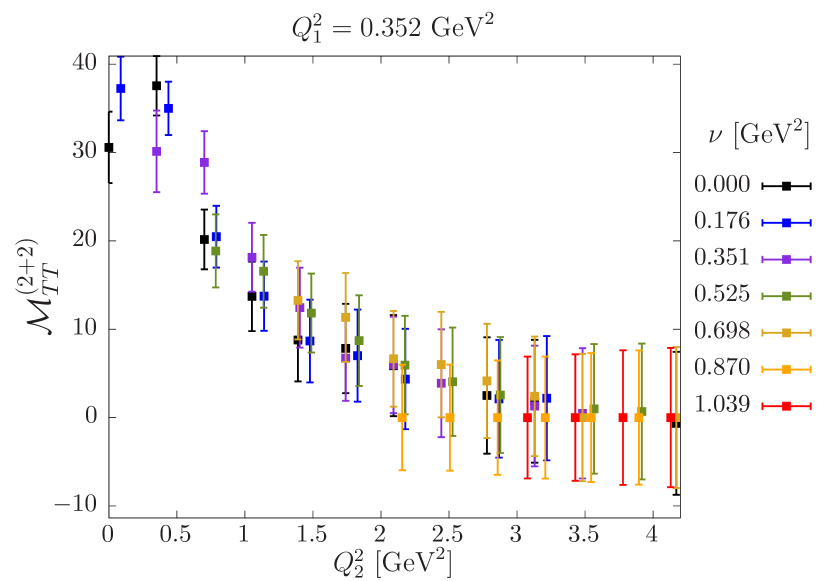
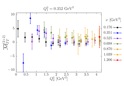
Figure 2: Contribution $(\times 10^{6})$ from $(2+2)$-disconnected diagrams to the forward scattering amplitude $\mathcal{M}_{TT}$ on ensemble E5, without (left) and with (right) subtraction of the value at $\nu=0$.

We now come to our results for the (2+2) disconnected diagram contribution to the eight subtracted amplitudes. We obtain this contribution with a reasonable statistical precision; however, some of the amplitudes are significantly different from zero when $Q^{2}_{2}=0$, as shown in the left panel of Fig. 2. In infinite volume, the Euclidean four-point function should vanish at this kinematic point, since a conserved current can be written as the divergence of a tensor field, $J_{\mu}(x)=\partial_{\nu}(x_{\mu}J_{\nu}(x))$, so that $\int d^{4}x\;J_{\mu}(x)$ is a pure boundary term, which vanishes in the presence of a mass gap. Therefore this is a sign of significant finite-volume effects. The bulk of the effect may be removed when subtracting the amplitude at $\nu=0$, but some of it may remain. Figure 2 also shows that due to correlations, the subtraction significantly reduces the statistical uncertainty. The full set of subtracted amplitudes on ensemble F6 is shown in Fig. LABEL:fig:22_F6.

V Empirical parametrization of the hadronic $\gamma^{*}\gamma^{*}$-fusion cross section

V.1 Model description and particle content

Table 2: Particle multiplets and physical values for the mass and two-photon width as quoted by the PDG Olive:2016xmw , as well as by Dai:2014zta for the two-photon width of the $f_{2}(1270)$ meson and Larin:2010kq for the $\pi^{0}$ width. In the case of the axial-vector mesons, the indicated width is the effective width defined in Eq. (77) and obtained phenomenologically in Danilkin:2016hnh . A cross indicates an absent or imprecise value in the PDG. An asterisk means that we use the isoscalar result divided by a factor 25/9 as explained in section III.2.

	Isovector			Isoscalar			Isoscalar
	name	$m$ [MeV]	$\Gamma_{\gamma\gamma}$ [keV]	name	$m$ [MeV]	$\Gamma_{\gamma\gamma}$ [keV]	name	$m$ [MeV]	$\Gamma_{\gamma\gamma}$ [keV]
$0^{-+}$	$\pi$	134.98	$0.0078(2)$	$\eta^{\prime}$	$957.78(6)$	$4.35(25)$	$\eta$	$547.86(2)$	$0.515(18)$
$0^{++}$	$a_{0}(980)$	$980(20)$	$0.30(10)$	$f_{0}(600)$	$\times$	$\times$	$f_{0}(980)$	$990(20)$	$0.31(5)$
$1^{++}$	$a_{1}(1260)$	$1230(40)$	$1.26^{*}$	$f_{1}(1285)$	$1281.8(0.6)$	$3.5(0.8)$	$f_{1}(1420)$	$1426.4(0.9)$	$3.2(0.9)$
$2^{++}$	$a_{2}(1320)$	$1318.3(0.6)$	$1.00(6)$	$f_{2}(1270)$	$1275.5(0.8)$	$2.93(40)$	$f_{2}^{\prime}(1525)$	$1525(5)$	$0.081(9)$

In this section, we describe how we model the hadronic $\gamma^{*}\gamma^{*}$-fusion cross section. We represent it as a sum of contributions from charge-conjugation even mesonic resonances produced in the $s$-channel. Specifically, we include the pseudoscalar ($J^{\rm PC}=0^{-+}$), scalar ($J^{\rm PC}=0^{++}$), axial-vector ($J^{\rm PC}=1^{++}$) and tensor ($J^{\rm PC}=2^{++}$) mesons. Table 2 lists the most relevant light mesons with these quantum numbers. In our implementation, we limit ourselves to the lightest state in each symmetry channel. The assumption that those states are sufficient to saturate the sum rules is motivated by the fact that, at small energies, higher mass singularities are suppressed in Eq. (9). Moreover, we have revised the model used in Green:2015sra to better account for the fact that we perform fits to the fully-connected diagrams. Rather than including isovector and isoscalar mesons, we consider only isovector mesons, enhanced by a factor $34/9$: we refer the reader to section III.2 for a justification of this approximation, which we expect to be superior. The procedure mostly modifies the contribution of the pseudoscalar sector, due to the large mass difference between the pion and the $\eta^{\prime}$ meson. Also, since lattice simulations are performed using $N_{f}=2$ dynamical quarks, we do not include the $\eta$ meson. Finally, we include the Born approximation to the $\gamma^{*}\gamma^{*}\to\pi^{+}\pi^{-}$ cross section using scalar QED, as described in Ref. Pascalutsa:2012pr , using a monopole vector form factor, the monopole mass being set to the $\rho$ meson mass. Explicit formulae for cross sections used in our model are given in Appendix A. The individual contributions to the eight amplitudes from each channel are summarized in Table 3.

Table 3: List of individual contributions to each of the eight helicity amplitudes. A cross indicates the absence of a contribution in the given channel. The relevant cross sections for each channel are given in Appendix A.

	$\mathcal{M}_{TT}$	$\mathcal{M}_{TT}^{\tau}$	$\mathcal{M}_{TT}^{a}$	$\mathcal{M}_{TL}$	$\mathcal{M}_{LT}$	$\mathcal{M}_{TL}^{\tau}$	$\mathcal{M}_{TL}^{a}$	$\mathcal{M}_{LL}$
Pseudoscalar	$\sigma_{0}/2$	$-\sigma_{0}$	$\sigma_{0}/2$	$\times$	$\times$	$\times$	$\times$	$\times$
Scalar	$\sigma_{0}/2$	$\sigma_{0}$	$\sigma_{0}/2$	$\times$	$\times$	$\tau_{TL}$	$\tau_{TL}$	$\sigma_{LL}$
Axial	$\sigma_{0}/2$	$-\sigma_{0}$	$\sigma_{0}/2$	$\sigma_{TL}$	$\sigma_{LT}$	$\tau_{TL}$	$-\tau_{TL}$	$\times$
Tensor	$\frac{\sigma_{0}+\sigma_{2}}{2}$	$\sigma_{0}$	$\frac{\sigma_{0}-\sigma_{2}}{2}$	$\sigma_{TL}$	$\sigma_{LT}$	$\tau_{TL}$	$\tau_{TL}^{a}$	$\sigma_{LL}$
Scalar QED	$\sigma_{TT}$	$\tau_{TT}$	$\tau_{TT}^{a}$	$\sigma_{TL}$	$\sigma_{LT}$	$\tau_{TL}$	$\tau_{TL}^{a}$	$\sigma_{LL}$

V.2 Assumptions on masses and resonances

Our lattice simulations are performed at larger-than-physical quark masses. For each ensemble, the pion and $\rho$ meson masses are determined from the pseudoscalar and vector two-point correlation functions respectively; see Table 1 for the obtained values. To obtain an estimate of the lowest-lying meson mass $m_{X}$ in every other symmetry channel, we assume that $m_{X}$ admits a constant additive shift relative to its physical value $m_{X}^{\mathrm{phys}}$. The shift $\delta m$ is determined from the difference between the $\rho$ mass computed on the lattice and its experimental value,

$$m_{X}=m_{X}^{\mathrm{phys}}+\delta m,\qquad\delta m=m_{\rho}^{\mathrm{lat}}-m_{\rho}^{\mathrm{phys}}\,.$$ (67)

In section VI, we will test the sensitivity of our results to variations of $\delta m$ by a factor of two. As for resonances, we assume that their contributions are well approximated by Breit-Wigner distributions and use the following formal substitution in the cross sections given in Appendix A,

$$\delta(s-m_{X}^{2})\ \leftrightarrow\ \frac{m_{X}}{\pi}\frac{\Gamma_{X}}{(s-m_{X}^{2})^{2}+m_{X}^{2}\Gamma_{X}^{2}}\,,$$ (68)

where $m_{X}$ and $\Gamma_{X}$ are the mass and the total width of the particle respectively. However, the remaining part of the cross section is still evaluated at $s=m_{X}^{2}$. For the (very narrow) pseudoscalar mesons, one can perform the integration explicitly and obtain the following contribution to the sum rules (using $\delta(\nu-\nu_{P})=2\delta(s-s_{P})$, where $\nu_{P}=\frac{1}{2}(m_{P}^{2}+Q_{1}^{2}+Q_{2}^{2})$) :

$$\frac{4\nu^{2}}{\pi}\int_{\nu_{0}}^{\infty}\!\!d\nu^{\prime}\,\frac{\sqrt{X^{\prime}}\sigma_{0}(\nu^{\prime})}{\nu^{\prime}(\nu^{\prime\,2}-\nu^{2}-i\epsilon)} =64\pi\ \frac{\Gamma_{\gamma\gamma}}{m_{P}}\ \frac{\nu^{2}X_{P}}{m_{P}^{2}\,\nu_{P}(\nu_{P}^{2}-\nu^{2})}\left[\frac{F_{{\cal P}\gamma^{\ast}\gamma^{\ast}}(Q_{1}^{2},Q_{2}^{2})}{F_{{\cal P}\gamma^{\ast}\gamma^{\ast}}(0,0)}\right]^{2}$$ (69)

$$=16\pi^{2}\alpha^{2}\ \frac{\nu^{2}X_{P}}{\nu_{P}(\nu_{P}^{2}-\nu^{2})}\left[F_{{\cal P}\gamma^{\ast}\gamma^{\ast}}(Q_{1}^{2},Q_{2}^{2})\right]^{2}\,,$$ (70)

in the even case, and

$$\frac{4\nu^{3}}{\pi}\int_{\nu_{0}}^{\infty}\!\!d\nu^{\prime}\,\frac{\sqrt{X^{\prime}}\sigma_{0}(\nu^{\prime})}{\nu^{\prime 2}(\nu^{\prime\,2}-\nu^{2}-i\epsilon)} =16\pi^{2}\alpha^{2}\ \frac{\nu^{3}X_{P}}{\nu_{P}^{2}(\nu_{P}^{2}-\nu^{2})}\left[F_{{\cal P}\gamma^{\ast}\gamma^{\ast}}(Q_{1}^{2},Q_{2}^{2})\right]^{2}\,,$$ (71)

in the odd case, where $X_{P}\equiv\nu_{P}^{2}-Q_{1}^{2}Q_{2}^{2}$.

V.3 Parametrization of the form factors

In this subsection, we briefly review the available information on the transition form factors of the exchanged mesons in the hadronic model, and present the parametrization we use in fitting the lattice HLbL amplitudes. While detailed information is available in the case of the pion from lattice QCD, no experimental data is presently available at doubly virtual kinematics in any channel. In these cases, a monopole or dipole ansatz, in which the $Q_{1}^{2}$ and $Q_{2}^{2}$ dependence factorizes, is made to describe the photon-virtuality dependence, even though such an ansatz might not have the asymptotic behavior predicted by the operator-product expansion. Our motivation is that this type of parametrization is used in model calculations of $a_{\mu}^{\rm HLbL}$. Also, given our goal of performing fits to the HLbL amplitudes computed on the lattice, the number of free parameters characterizing the transition form factors should be commensurate with the precision of the lattice data.

V.3.1 Pseudoscalar mesons

For pseudoscalar mesons, experimental data are available when at least one photon is on-shell, and in this case a good parametrization of the data is obtained using a monopole form factor Behrend:1990sr ; Gronberg:1997fj ; Aubert:2009mc ; Uehara:2012ag . However, as shown in Ref. Gerardin:2016cqj , a monopole form factor failed to reproduce the lattice data in the doubly-virtual case, in contrast to the LMD+V model. Furthermore, the LMD+V model is compatible with the Brodsky-Lepage behavior Lepage:1979zb ; Lepage:1980fj ; Brodsky:1981rp in the singly-virtual case and with the operator-product expansion (OPE) prediction Nesterenko:1982dn ; Novikov:1983jt in the $Q_{1}^{2}=Q_{2}^{2}$ doubly-virtual case. We therefore use this model for the pion transition form factor, of which the parameters were determined in Ref. Gerardin:2016cqj for each ensemble listed in Table 1.

V.3.2 Scalar mesons

Scalar mesons can be produced by two transverse (T) or two longitudinal (L) photons. Correspondingly, the amplitude is parametrized by two form factors, $F^{T}_{{\cal S}\gamma^{\ast}\gamma^{\ast}}$ and $F^{L}_{{\cal S}\gamma^{\ast}\gamma^{\ast}}$. Only the first one has been measured experimentally: this was done for the $f_{0}(980)$ meson in the region $Q^{2}<30{\rm\,GeV}^{2}$ by the Belle Collaboration Masuda:2015yoh , and the results are compatible with a monopole form factor with a monopole mass $M_{S}=0.800(50)\leavevmode\nobreak\ \mathrm{GeV}$. Therefore, we assume the form

$$\frac{F^{T}_{{\cal S}\gamma^{\ast}\gamma^{\ast}}(Q_{1}^{2},Q_{2}^{2})}{F^{T}_{{\cal S}\gamma^{\ast}\gamma^{\ast}}(0,0)}=\frac{1}{(1+Q_{1}^{2}/M_{S}^{2})(1+Q_{2}^{2}/M_{S}^{2})}\,.$$ (72)

For simplicity, we also assume that the transverse and longitudinal form factors are equal (the longitudinal one is only relevant for the amplitudes $M^{a}_{TL}$, $M^{\tau}_{TL}$ and $M_{LL}$),

$${F^{L}_{{\cal S}\gamma^{\ast}\gamma^{\ast}}(Q_{1}^{2},Q_{2}^{2})=-F^{T}_{{\cal S}\gamma^{\ast}\gamma^{\ast}}(Q_{1}^{2},Q_{2}^{2})\,.}$$ (73)

The normalization is obtained from the experimentally measured two-photon decay width $\Gamma_{\gamma\gamma}$ given by (see Table 2)

$$\Gamma_{\gamma\gamma}=\frac{\pi\alpha^{2}}{4}m_{S}\left[F^{T}_{{\cal S}\gamma^{\ast}\gamma^{\ast}}(0,0)\right]^{2}\,,$$ (74)

while the monopole mass $M_{S}$ will be treated as a free parameter.

V.3.3 Axial mesons

For axial mesons, we have two form factors, $F^{(0)}_{{\cal A}\gamma^{\ast}\gamma^{\ast}}$ and $F^{(1)}_{{\cal A}\gamma^{\ast}\gamma^{\ast}}$, corresponding to the two helicity states of the meson. We use the same parametrization as in Ref. Pascalutsa:2012pr , inspired by quark models,

$$F^{(0)}_{{\cal A}\gamma^{\ast}\gamma^{\ast}}(Q_{1}^{2},Q_{2}^{2}) =m_{A}^{2}A(Q_{1}^{2},Q_{2}^{2})\,,$$ (75a)

$$F^{(1)}_{{\cal A}\gamma^{\ast}\gamma^{\ast}}(Q_{1}^{2},Q_{2}^{2}) =-\frac{\nu}{X}\left(\nu+Q_{2}^{2}\right)\,m_{A}^{2}A(Q_{1}^{2},Q_{2}^{2})\,,$$ (75b)

$$F^{(1)}_{{\cal A}\gamma^{\ast}\gamma^{\ast}}(Q_{2}^{2},Q_{1}^{2}) =-\frac{\nu}{X}\left(\nu+Q_{1}^{2}\right)\,m_{A}^{2}A(Q_{1}^{2},Q_{2}^{2})\,,$$ (75c)

in which $2\nu=m_{A}^{2}+Q_{1}^{2}+Q_{2}^{2}$ with $m_{A}$ the meson mass,

$$\frac{A(Q_{1}^{2},0)}{A(0,0)}=\frac{1}{(1+Q_{1}^{2}/M_{A}^{2})^{2}}\,,$$ (76)

and assuming factorization such that $A(Q_{1}^{2},Q_{2}^{2})=A(Q_{1}^{2},0)A(0,Q_{2}^{2})/A(0,0)=A(Q_{2}^{2},Q_{1}^{2})$. In particular, the form factor $F^{(1)}_{{\cal A}\gamma^{\ast}\gamma^{\ast}}$ is not symmetric in the photon virtualities $Q_{1}^{2},Q_{2}^{2}$. These form factors have been measured by the L3 Collaboration for one real and one virtual photon in the region $Q^{2}<5\leavevmode\nobreak\ \mathrm{GeV}^{2}$ Achard:2001uu ; Achard:2007hm for the isoscalar resonance. Using the previous parametrization, the authors obtain the dipole mass $M_{A}=1040(78)\leavevmode\nobreak\ \mathrm{MeV}$ for the $f_{1}(1285)$ meson. We obtain the normalization of the form factors from the values given in Danilkin:2016hnh for the effective two-photon width, defined as

$$\tilde{\Gamma}_{\gamma\gamma}\equiv\lim_{Q_{1}^{2}\to 0}\frac{m_{A}^{2}}{Q_{1}^{2}}\frac{1}{2}\Gamma(\mathcal{A}\to\gamma_{L}^{*}\gamma_{T})=\frac{\pi\alpha^{2}}{4}\frac{m_{A}}{3}\left[F^{(1)}_{{\cal A}\gamma^{\ast}\gamma^{\ast}}(0,0)\right]^{2}\,,$$ (77)

and we will consider $M_{A}$ as a free parameter in our fits.

Table 4: Tensor form factor normalizations for the isoscalar meson $f_{2}(1270)$. For helicities $\Lambda=2$ and $\Lambda=(0,T)$ the normalization is obtained using Eq. (79) and the measured two-photon decay width. For helicities $\Lambda=1$ and $\Lambda=(0,L)$ the results are extracted from Ref. Danilkin:2016hnh .

	$\Lambda=2$	$\Lambda=(0,T)$	$\Lambda=1$	$\Lambda=(0,L)$
$F^{(\Lambda)}_{{\cal T}\gamma^{\ast}\gamma^{\ast}}(0,0)$	$0.500\pm 0.034$	$0.095\pm 0.011$	$0.24\pm 0.05$	$-0.90\pm 0.30$

V.3.4 Tensor mesons

We now turn our attention to the tensor mesons. The singly-virtual form factors of the isoscalar resonance $f_{2}$ for helicities $\Lambda=2,1,(0,T)$ have also been measured experimentally in the region $Q^{2}<30\leavevmode\nobreak\ \mathrm{GeV}^{2}$ by the Belle Collaboration Masuda:2015yoh , where the data are compatible with a dipole form factor Danilkin:2016hnh . Therefore, we use the following parametrization for all helicities $\Lambda=(0,T),(0,L),1,2$,

$$\frac{F^{(\Lambda)}_{{\cal T}\gamma^{\ast}\gamma^{\ast}}(Q_{1}^{2},Q_{2}^{2})}{F^{(\Lambda)}_{{\cal T}\gamma^{\ast}\gamma^{\ast}}(0,0)}=\frac{1}{(1+Q_{1}^{2}/M_{T,(\Lambda)}^{2})^{2}(1+Q_{2}^{2}/M_{T,(\Lambda)}^{2})^{2}}\,,$$ (78)

where we allow for a different dipole mass for each helicity. The normalization of the transverse form factors is computed from the experimentally measured two-photons widths Olive:2016xmw , $\Gamma_{\gamma\gamma}=\Gamma_{\gamma\gamma}^{(0)}+\Gamma_{\gamma\gamma}^{(2)}$, assuming that the ratio of helicity 2 to helicity 0 decays is $r=91.3\leavevmode\nobreak\ \%$ (see Ref. Dai:2014lza ):

$$\Gamma_{\gamma\gamma}^{(0)} ={\pi\alpha^{2}}\,m_{T}\,\frac{2}{15}\,\left[F^{(0,T)}_{{\cal T}\gamma^{\ast}\gamma^{\ast}}(0,0)\right]^{2}\,,$$

$$\Gamma_{\gamma\gamma}^{(2)} =\frac{\pi\alpha^{2}}{4}\,m_{T}\,\frac{1}{5}\,\left[F^{(2)}_{{\cal T}\gamma^{\ast}\gamma^{\ast}}(0,0)\right]^{2}\,.$$ (79)

In Ref. Danilkin:2016hnh , the authors obtain the normalization of the two other form factors by saturating two different sum rules involving one real and one virtual photon; their results are summarized in Table 4.

Finally, based on large-$N$ arguments reviewed in section III.2, we assume the following relationship between the two-photon decay widths of the isoscalar and isovector mesons,

$$\Gamma_{\gamma\gamma}(f_{X})=\frac{25}{9}\,\Gamma_{\gamma\gamma}(a_{X})\,.$$ (80)

In particular, we observe that this approximation works well for the tensor meson, where the two-photon decay widths have been measured both for the isovector and isoscalar mesons (see Table 2).

VI Fitting the $\gamma^{*}\gamma^{*}\to\,$hadrons model to the lattice HLbL amplitudes

VI.1 Preliminary checks

In this section, we fit simultaneously the eight forward light-by-light amplitudes using the phenomenological model described in Sec. V. We have checked that we can reproduce the results given in Refs. Pascalutsa:2012pr ; Danilkin:2016hnh in the limit where only one photon is virtual to the quoted accuracy  (Tables I and II of Pascalutsa:2012pr and Table III and IV of Danilkin:2016hnh ). Moreover, fits have been checked using two different routines: the Minuit package from CERN Minuit and the GSL library GSL .

VI.2 Fit of the eight helicity amplitudes

It appears that the five subtracted amplitudes $\overline{\mathcal{M}}_{TT}$, $\overline{\mathcal{M}}_{TT}^{\tau}$, $\overline{\mathcal{M}}_{TT}^{a}$, $\overline{\mathcal{M}}_{TL}$ and $\overline{\mathcal{M}}_{LT}$ are statistically more precise than the three other amplitudes $\overline{\mathcal{M}}_{TL}^{\tau}$, $\overline{\mathcal{M}}_{TL}^{a}$ and $\overline{\mathcal{M}}_{LL}$. Moreover, these last three amplitudes also depend on the longitudinal scalar form factor and on the tensor form factor with helicity $\Lambda=(0,L)$ which are unknown from experiment and for which we use values from phenomenology (see Table 4). As shown in the last row of Table 6, the contribution from scalar QED is always small and therefore we do not try to fit the associated monopole mass which is explicitly set to the rho mass computed on the lattice. We therefore have six fit parameters, which correspond to the monopole and dipole masses of the scalar ($M_{S}$), axial ($M_{A}$) and tensor ($M^{(2)}_{T},M^{(0,T)}_{T},M^{(1)}_{T},M^{(0,L)}_{T}$) mesons. The results are given in Table 5, and the corresponding plots for the ensemble F6 are shown in Figs. (LABEL:fig:amps_F6_part1 and LABEL:fig:amps_F6_part2; additional plots for G8 are shown in appendix B, LABEL:fig:amps_G8_part1). The quoted error on the fit parameters is only statistical and estimated using the jackknife method. The quoted $\chi^{2}$ correspond to uncorrelated fits. The $\chi^{2}$ per degree of freedom are slightly above unity, with the exception of the value for ensemble E5. Here we attribute its large value to the fact that the statistical errors are smallest on E5 and that finite-volume effects could be significant for this ensemble. Given that lattice artifacts and finite-size effects are not taken into account by the $\chi^{2}$, we consider the obtained description of the data on the other ensembles to be satisfactory.

In Table 6, we show the relative contribution of each channel to the different amplitudes at $Q_{1}^{2}=0.352\leavevmode\nobreak\ \mathrm{GeV}^{2}$, $\nu=0.467\leavevmode\nobreak\ \mathrm{GeV}^{2}$ and for two values of $Q_{2}^{2}$. The amplitudes $\overline{\mathcal{M}}_{TT}^{a}$, $\overline{\mathcal{M}}_{TT}^{\tau}$, $\overline{\mathcal{M}}_{TL}^{\tau}$ and $\overline{\mathcal{M}}_{TL}^{a}$ involve interference cross sections and are not sign-definite: we observe large cancellations between the different contributions. The latter help to stabilize the fit due to the enhanced sensitivity to the relative size of these contributions. In particular, fitting only the amplitudes $\overline{\mathcal{M}}_{TT}$, $\overline{\mathcal{M}}_{TL}$ and $\overline{\mathcal{M}}_{LT}$ leads to unstable fits. Figures LABEL:fig:nu_G8_part1 and LABEL:fig:nu_G8_part2, in addition to displaying the $\nu$-dependence of the amplitudes for two sets of values of $(Q_{1}^{2},Q_{2}^{2})$, show the contributions of the individual mesons. The pseudoscalar and tensor mesons give the dominant contribution to the amplitudes $\overline{\mathcal{M}}_{TT}$, $\overline{\mathcal{M}}_{TT}^{\tau}$ and $\overline{\mathcal{M}}_{TT}^{a}$, which involve two transverse photons. As stated above, the scalar QED contribution is always small, except for $\overline{\mathcal{M}}_{LL}$. The axial form factor is mainly constrained from $\overline{\mathcal{M}}_{TL}$, $\overline{\mathcal{M}}_{LT}$ where the axial and tensor mesons make the dominant contribution; this is clearly visible from Figs. LABEL:fig:nu_G8_part1 and LABEL:fig:nu_G8_part2. It also contributes significantly to the amplitudes $\overline{\mathcal{M}}_{TL}^{a}$ and $\overline{\mathcal{M}}_{TL}^{\tau}$, which involve one transverse and one longitudinal photon. On the other hand, the axial meson does not contribute significantly to the amplitudes $\overline{\mathcal{M}}_{TT}$, $\overline{\mathcal{M}}_{TT}^{\tau}$ and $\overline{\mathcal{M}}_{TT}^{a}$ involving two transverse photons, especially at low virtualities. This suppression is expected since axial mesons have vanishing contribution when at least one photon is real according to the Landau-Yang theorem Landau:1948kw ; Yang:1950rg . Finally, the tensor meson contributes significantly to all amplitudes.

Table 5: Results of the simultaneous fit to the eight subtracted amplitudes $\overline{\mathcal{M}}_{TT}$, $\overline{\mathcal{M}}_{TT}^{\tau}$, $\overline{\mathcal{M}}_{TT}^{a}$, $\overline{\mathcal{M}}_{TL}$, $\overline{\mathcal{M}}_{LT}$, $\overline{\mathcal{M}}_{TL}^{a}$, $\overline{\mathcal{M}}_{TL}^{\tau}$ and $\overline{\mathcal{M}}_{LL}$ for the five lattice ensembles. The six mass parameters are given in units of GeV.

	$M_{S}$	$M_{A}$	$M^{(2)}_{T}$	$M^{(0,T)}_{T}$	$M^{(1)}_{T}$	$M^{(0,L)}_{T}$	$\chi^{2}/\mathrm{d.o.f.}$
E5	1.38(11)	1.26(10)	1.93(3)	2.24(5)	2.36(4)	0.60(10)	4.22
F6	1.12(14)	1.44(5)	1.66(9)	2.17(5)	1.85(14)	0.89(28)	1.15
F7	1.04(18)	1.29(8)	1.61(12)	2.08(7)	2.03(7)	0.57(16)	1.19
G8	1.07(10)	1.36(5)	1.37(24)	2.03(6)	1.63(13)	0.73(14)	1.13
N6	0.86(37)	1.59(3)	1.72(17)	2.19(4)	1.72(18)	0.51(8)	1.35

Table 6: Relative contributions in % of each particle to the different amplitudes for the ensemble F7 at $Q_{1}^{2}=0.352\leavevmode\nobreak\ \mathrm{GeV}^{2}$, $\nu=0.467\leavevmode\nobreak\ \mathrm{GeV}^{2}$ and for two values of $Q_{2}^{2}$. For each $Q_{2}^{2}$ value, the normalization is such that the absolute values of the entries in a given column add up to 100.

	$Q_{2}^{2}\leavevmode\nobreak\ [\mathrm{GeV}^{2}]$	$\overline{\mathcal{M}}_{TT}$	$\overline{\mathcal{M}}_{TT}^{\tau}$	$\overline{\mathcal{M}}_{TT}^{a}$	$\overline{\mathcal{M}}_{TL}$	$\overline{\mathcal{M}}_{LT}$	$\overline{\mathcal{M}}_{TL}^{a}$	$\overline{\mathcal{M}}_{TL}^{\tau}$	$\overline{\mathcal{M}}_{LL}$
$0^{-+}$	1.0	35	$-56$	68	$\times$	$\times$	$\times$	$\times$	$\times$
	3.0	30	$-38$	61	$\times$	$\times$	$\times$	$\times$	$\times$
$0^{++}$	1.0	7	11	8	$\times$	$\times$	23	14	42
	3.0	5	6	8	$\times$	$\times$	19	9	50
$1^{++}$	1.0	2	$-2$	1	43	57	$-43$	32	$\times$
	3.0	8	$-11$	11	21	49	$-40$	23	$\times$
$2^{++}$	1.0	53	25	$-20$	56	42	19	$-47$	25
	3.0	56	44	19	79	51	$-38$	$-67$	40
Scalar QED	1.0	4	5	3	1	$<1$	$-15$	$-7$	33
	3.0	1	1	1	$<1$	$<1$	$-3$	$-1$	10

VI.3 Influence of the non-fitted model parameters

In the previous fit, only the monopole and dipole masses entering the form factors were considered as fit parameters. The other parameters ($p=\Gamma,\Gamma_{\gamma\gamma},\delta m,\dots$) were fixed using phenomenology as described in Sec. V. However, these parameters are sometimes associated with relatively large experimental errors ($\delta p$) or modelled (like the global mass shift in the spectrum where we assume $m_{X}=m_{X}^{\exp}+\delta m$ with $\delta m=m_{\rho}^{\rm lat}-m_{\rho}^{\exp}$). Therefore, we perform exactly the same fit as in the previous section but using $p\pm\delta p$ instead of $p$ (and varying only one parameter at a time). In this way, we can see the influence of these parameters on the monopole and dipole masses obtained in the previous section. The results are summarized in Table 7 for the ensemble F6. In this table, $\delta m$ corresponds to the global mass shift applied to the spectrum (see Eq. (67)), and is multiplied or divided by a factor of two.

We observe that the experimental error on the total decay widths of the particles have a negligible effect. Increasing the two-photon width (or equivalently, the normalization of the form factor) tends to reduce the associated monopole or dipole mass. Finally, increasing the global mass shift by a factor two leads to a noticeable change in the monopole and dipole masses with little change in the $\chi^{2}$.

Varying the normalization of the form factor $F_{{\cal T}\gamma^{*}\gamma^{*}}^{(0,L)}$ leads to negligible changes in all parameters but $M_{T}^{(0,L)}$; this particular correlation is studied in more detail in the next subsection.

Table 7: Fit variations for F6. The first row corresponds to the results obtained in the previous section. Then, each row corresponds to a new fit using $p\pm\delta p$ and varying only one parameter at a time: the quoted number is the shift observed for the monopole/dipole mass, in units of GeV. A cross indicates that the parameter remains unchanged to all indicated digits of the central values in the first row. For instance, using $\Gamma_{\gamma\gamma}(a_{0})+\delta\Gamma_{\gamma\gamma}(a_{0})$ instead of $\Gamma_{\gamma\gamma}(a_{0})$, the scalar monopole mass is shifted by $-0.09\leavevmode\nobreak\ \mathrm{GeV}$, the other monopole/dipole masses being unaffected. In the last row, the mass shift $\delta m$ applied to the spectrum (see Eq. (67)) is varied by a factor of two.

	$M_{S}$	$M_{A}$	$M^{(2)}_{T}$	$M^{(0,T)}_{T}$	$M^{(1)}_{T}$	$M^{(0,L)}_{T}$	$\chi^{2}/\mathrm{d.o.f.}$
Principal	$1.12(14)$	1.44(5)	1.66(9)	2.17(5)	1.85(14)	0.91(7)	1.15
$\Gamma(a_{0})$	$\times$	$\times$	$\times$	$\times$	$\times$	$\times$	1.15
	$\times$	$\times$	$\times$	$\times$	$\times$	$\times$	1.15
$\Gamma_{\gamma\gamma}(a_{0})$	$-0.09$	$\times$	$\times$	$\times$	$\times$	$\times$	1.14
	$+0.12$	$\times$	$\times$	$\times$	$\times$	$\times$	1.15
$\Gamma(a_{1})$	$-0.01$	$+0.03$	$\times$	$+0.01$	$\times$	$\times$	1.14
	$-0.01$	$-0.02$	$+0.01$	$\times$	$+0.01$	$\times$	1.15
$\tilde{\Gamma}_{\gamma\gamma}(a_{1})$	$\times$	$-0.10$	$+0.02$	$-0.01$	$+0.02$	$\times$	1.17
	$+0.03$	$+0.19$	$-0.01$	$+0.02$	$-0.01$	$\times$	1.12
$\Gamma(a_{2})$	$\times$	$\times$	$\times$	$\times$	$\times$	$\times$	1.15
	$\times$	$\times$	$\times$	$\times$	$\times$	$\times$	1.15
$F_{{\cal T}\gamma^{*}\gamma^{*}}^{(2)}$	$-0.01$	$\times$	$-0.06$	$+0.01$	$\times$	$\times$	1.15
	$\times$	$\times$	$+0.08$	$\times$	$+0.01$	$\times$	1.14
$F_{{\cal T}\gamma^{*}\gamma^{*}}^{(0,T)}$	$-0.08$	$\times$	$-0.01$	$-0.09$	$-0.01$	$\times$	1.13
	$+0.08$	$\times$	$+0.02$	$+0.11$	$+0.02$	$\times$	1.17
$F_{{\cal T}\gamma^{*}\gamma^{*}}^{(1)}$	$\times$	$\times$	$\times$	$\times$	$-0.14$	$\times$	1.14
	$-0.01$	$\times$	$\times$	$\times$	$+0.21$	$\times$	1.15
$\delta m^{\times 2}_{\times 0.5}$	$+0.20$	$+0.13$	$+0.11$	$+0.13$	$+0.14$	$+0.10$	1.17
	$-0.10$	$-0.06$	$-0.05$	$-0.08$	$-0.06$	$-0.05$	1.15

VI.4 Bounds for the tensor form factor $F_{{\cal T}\gamma^{*}\gamma^{*}}^{(0,L)}$

The transition form factor $F_{{\cal T}\gamma^{*}\gamma^{*}}^{(0,L)}$ of the tensor meson enters only the amplitudes $\mathcal{M}_{TL}^{\tau}$, $\mathcal{M}_{TL}^{a}$ and $\mathcal{M}_{LL}$, which are less precisely determined on the lattice. In particular the fit is not able to determine both the dipole mass and the normalization independently, and they are highly correlated. To illustrate this point, we use the previously obtained best fit parameters and compute the $\chi^{2}/\mathrm{d.o.f.}$ along a scan in the plane ($M_{T}^{(0,L)}$, $F_{{\cal T}\gamma^{*}\gamma^{*}}^{(0,L)}(0,0)$). The results are shown in Fig. 3: for a dipole mass of $1\leavevmode\nobreak\ \mathrm{GeV}$, a normalization $F_{{\cal T}\gamma^{*}\gamma^{*}}^{(0,L)}(0,0)\approx-0.4$ is favored but the results show a strong dependence on $M_{T}^{(0,L)}$.

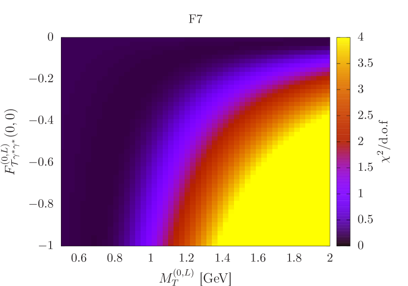
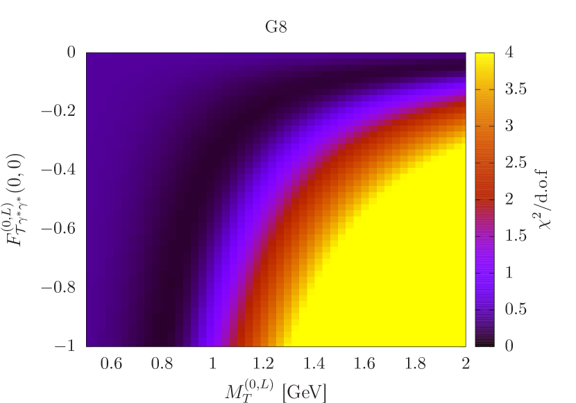
Figure 3: Value of $\chi^{2}/\mathrm{d.o.f.}$ for different dipole masses and form factor normalizations (tensor form factor, helicity $\Lambda=(0,L)$). Left: ensemble F7, right: ensemble G8.

VI.5 Chiral extrapolations

Finally, we perform a chiral extrapolation for the six monopole and dipole masses that we have fitted to the lattice four-point function. For each of these parameters, we assume a linear dependence on $m_{\pi}^{2}$. We perform two sets of fits, either including or excluding the ensemble E5, which has the largest pion mass. The lattice results are given in Table 8 and depicted in Fig. 4 together with the fits excluding E5. The displayed errors are purely statistical. The blue points in Fig. 4 represent the ensemble N6 and therefore correspond to a finer lattice spacing than the other data points. We remind the reader that we have included only isovector mesons in the description of the fully connected amplitude, therefore all our fitted form factor parameters correspond to isovector mesons. While the results are quite stable under including or excluding ensemble E5, we consider the latter to be our final results, mainly because the $\chi^{2}$ per degree of freedom of the global fit was unacceptably large for E5. We make the following observations:

• The monopole mass of the scalar meson transition form factor does not depend strongly on the pion mass. After a mild extrapolation, we obtain $M_{S}=1.04(14)\leavevmode\nobreak\ \mathrm{GeV}$ at the physical pion mass. The result lies above the experimental result $M_{S}=0.796(54)\leavevmode\nobreak\ \mathrm{GeV}$ from the Belle Collaboration for the isoscalar scalar meson Masuda:2015yoh .

• The axial dipole mass is also very weakly dependent on the pion mass. We obtain $M_{A}=1.32(7)\leavevmode\nobreak\ \mathrm{GeV}$ at the physical pion mass.

  Table 8: Results of the chiral extrapolation for the scalar monopole mass $M_{S}$, the axial dipole mass $M_{A}$ and the four tensor dipole masses corresponding to different helicities. All results are given in units of GeV and correspond to isovector mesons at the physical value of the pion mass. Results including or excluding the ensemble (E5) with the largest pion mass are given. We consider the latter to be our final results (last column of the table).

  
  

  	Including E5	Excluding E5
  $M_{S}$	0.94(12)	1.04(14)
  $M_{A}$	1.40(07)	1.32(07)
  $M_{T}^{(2)}$	1.39(12)	1.35(24)
  $M_{T}^{(1)}$	1.67(10)	1.69(16)
  $M_{T}^{(0,T)}$	2.01(07)	1.96(09)
  $M_{T}^{(0,L)}$	0.74(14)	0.67(19)

  The finer ensemble N6 suggests a value $10\%$ larger. More ensembles would be needed to confirm whether $M_{A}$ is afflicted by large discretisation effects. For comparison, the L3 Collaboration obtained a dipole mass $M_{A}=1.040(80)\leavevmode\nobreak\ \mathrm{GeV}$ for the isoscalar partner $f_{1}(1285)$; the measurement relied on single-virtual measurements only Achard:2001uu ; Achard:2007hm . The difference in the kinematics at which the form factor was probed could be part of the reason we found a larger dipole mass, in addition to a potential genuine difference between the isospin partners. We also recall that the transition form factors have been parametrized in a fairly simplistic way (see Eq. (76) and above).

• Finally, for the tensor meson $a_{2}$, linear extrapolations in $m_{\pi}^{2}$ yield the results given in Table 8. Fits to experimental data on the single-virtual form factor Masuda:2015yoh ; Danilkin:2016hnh yielded smaller values for the $f_{2}(1270)$ meson. For instance, our result for the helicity-2 transition form factor, $M_{T}^{(2)}=1.35(24)\leavevmode\nobreak\ \mathrm{GeV}$, is only slightly larger than the value $1.222(66)\leavevmode\nobreak\ \mathrm{GeV}$ obtained phenomenologically. On the other hand, our values of $M_{T}^{(1)}=1.69(16)\leavevmode\nobreak\ \mathrm{GeV}$ and $M_{T}^{(0,T)}=1.96(9)\leavevmode\nobreak\ \mathrm{GeV}$ are almost a factor two larger than the corresponding phenomenological $f_{2}$ results, $M_{T}^{(1)}=0.916(20)\leavevmode\nobreak\ \mathrm{GeV}$ and $M_{T}^{(0,T)}=1.051(36)\leavevmode\nobreak\ \mathrm{GeV}$. Especially $M_{T}^{(0,T)}$ is statistically well constrained by the lattice data and only weakly dependent on the lattice spacing and the pion mass. Finally, our value for $M_{T}^{(0,L)}=0.67(19)\leavevmode\nobreak\ \mathrm{GeV}$ is in agreement with the estimate $0.877(66)\leavevmode\nobreak\ \mathrm{GeV}$ obtained in Danilkin:2016hnh within the large uncertainties.

To summarize, in all cases except $M_{T}^{(0,L)}$, we obtain larger monopole and dipole masses for the isovector mesons than in phenomenology for the isoscalar mesons. The strongest difference is in $M_{T}^{(1)}$ and $M_{T}^{(0,T)}$, where we find that the form factors fall off far more slowly; this discrepancy could be due to the use of the factorization assumption for the dependence on the photon virtualities. On the other hand, we find agreement within the uncertainties for the scalar monopole mass and the helicity-two form factor of the tensor meson.

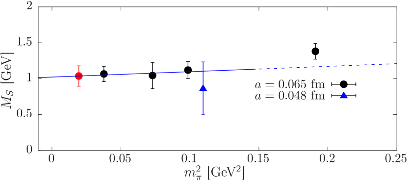
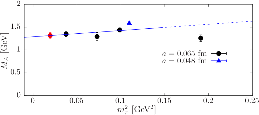
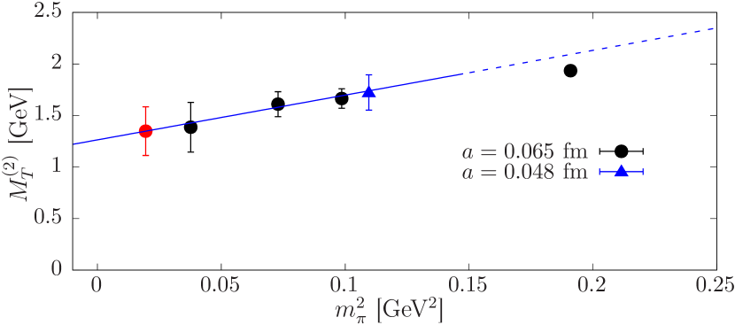
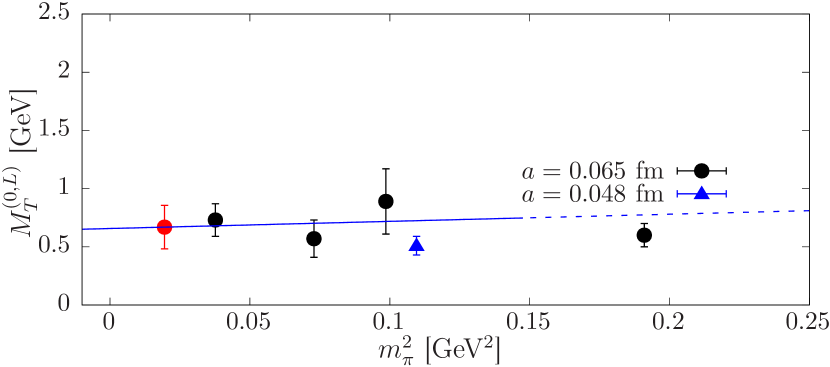
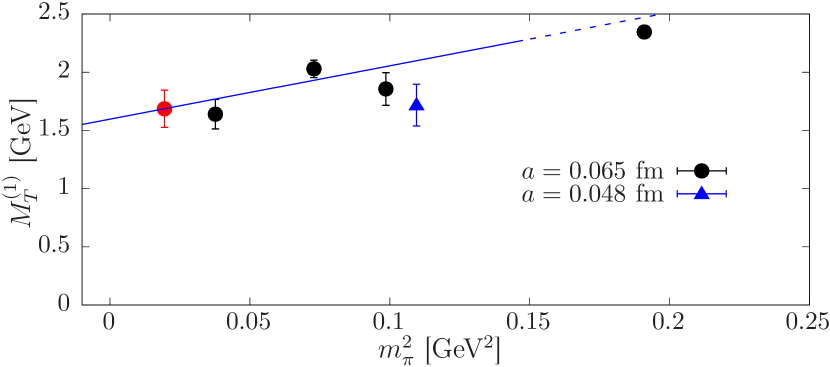
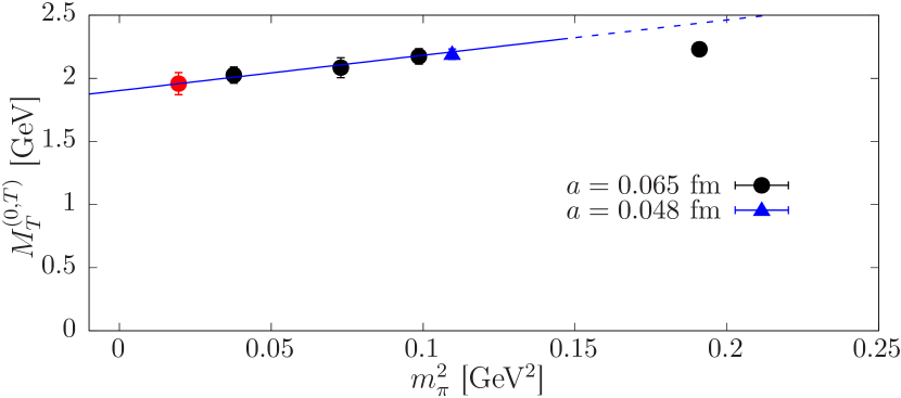
Figure 4: Chiral extrapolations for each monopole and dipole mass, excluding the ensemble E5 with the largest pion mass. The blue point corresponds to the lattice ensemble N6 and gives an indication about discretisation effects. Only the statistical error is displayed.

VII Study of disconnected diagrams

In this section, we test whether the hadronic model of section V together with the arguments summarized in section III.2 is consistent with the (2+2) disconnected diagrams, which we have computed on two lattice ensembles. The arguments, based on the large-$N$ motivated idea that an isolated vector current insertion in a fermion loop gives a suppressed contribution, lead to the conclusion that the (2+2) disconnected class of diagrams contains all of the contributions from flavor-singlet meson poles, while the mesons in the adjoint representation of the flavor symmetry group contribute with a negative weight factor; the latter is $(-25/9)$ in the SU(2)_flavor case and $(-2)$ in the SU(3)_flavor case. The generic large-$N$ expectations would further lead to the stronger conclusion that, in each $J^{PC}$ sector, the non-singlet resonances cancel the contribution of the flavor-singlet resonances. One channel, however, where the degeneracy is badly broken is the pseudoscalar sector, since the pion is much lighter than the $\eta^{\prime}$ meson. Therefore, in the two-flavor theory we expect the (2+2) disconnected class of diagrams to be given to a good approximation by

$${\cal M}^{(2+2)}_{..}\approx-\frac{25}{9}{\cal M}^{(\pi^{0})}_{..}+{\cal M}^{(\eta^{\prime})}_{..}\;.$$ (81)

We have calculated the $\pi^{0}\to\gamma^{*}\gamma^{*}$ transition form factor on the same lattice ensembles as used here in a previous publication Gerardin:2016cqj . For the $\eta^{\prime}$, the two-photon decay width is fairly well known experimentally; thus, assuming a vector-meson-dominance model for the virtuality dependence of the $\eta^{\prime}$ transition form factor and using the known $\rho$ mass on each lattice ensemble, Eq. (81) provides a prediction for the ${\cal M}^{(2+2)}_{..}$ amplitudes. We use the vector mass given in Table 1. In Fig. LABEL:fig:22_F6 we display the prediction for the three largest subtracted amplitudes $\overline{\cal M}^{(2+2)}_{TT}$, $\overline{\cal M}^{\tau,(2+2)}_{TT}$ and $\overline{\cal M}^{a,(2+2)}_{TT}$ together with the direct lattice calculation. We find that Eq. (81) predicts the overall size of the amplitudes well, within the fairly large uncertainties. The agreement is most compelling in the $\overline{\cal M}^{\tau,(2+2)}_{TT}$ amplitude; this is also one of the amplitudes where the pseudoscalar poles make a large contribution. In fact, in this channel, $\overline{\cal M}^{\tau,(2+2)}_{TT}$ amounts to about $-90\%$ of the fully connected contribution $\overline{\cal M}^{\tau,(4)}_{TT}$.

VII.1 Estimate of the contribution of the (2+2) disconnected class of diagrams to $a_{\mu}^{\rm HLbL}$

We have obtained some evidence from our $N_{f}=2$ lattice data that the (2+2) class of diagrams is dominated by the pseudoscalar exchanges with the weight factors derived in section III.2. Using the results from Nyffeler:2016gnb , we can now estimate the importance of the $(2+2)$ disconnected class of diagrams in $a_{\mu}^{\rm HLbL}$ in two limits:

• $m_{s}=\infty$, which corresponds to the two-flavor theory;

• $m_{s}=m_{ud}$, which corresponds to the SU(3)-flavor symmetric theory.

We expect the real world to lie between these two predictions. In these two limits, we obtain

$$a_{\mu}^{\rm HLbL,(2+2)}\approx\left\{\begin{array}[]{l@{~~~~}l}-\frac{25}{9}a_{\mu}^{{\rm HLbL},\pi^{0}}+a_{\mu}^{{\rm HLbL},\eta^{\prime}}=-(162\pm 27)\cdot 10^{-11}\hfil\leavevmode\nobreak\ \leavevmode\nobreak\ \leavevmode\nobreak\ \leavevmode\nobreak\ &m_{s}=\infty,\phantom{\Big{|}}\\ -2(a_{\mu}^{{\rm HLbL},\pi^{0}}+a_{\mu}^{{\rm HLbL},\eta})+a_{\mu}^{{\rm HLbL},\eta^{\prime}}=-(142\pm 19)\cdot 10^{-11}\hfil\leavevmode\nobreak\ \leavevmode\nobreak\ \leavevmode\nobreak\ \leavevmode\nobreak\ &m_{s}=m_{ud}.\phantom{\Big{|}}\end{array}\right.$$ (82)

We have used the LMD+V result for the pion ($62.9\cdot 10^{-11}$) and the VMD results for the $\eta$ and $\eta^{\prime}$ (respectively $14.5\cdot 10^{-11}$ and $12.5\cdot 10^{-11}$) quoted in Nyffeler:2016gnb (see also References therein) and assigned to each contribution an uncertainty of $15\%$. For comparison, the $N_{f}=2$ lattice calculation Gerardin:2016cqj of the pion transition form factor and its parametrization by the LMD+V model led to the value $a_{\mu}^{{\rm HLbL},\pi^{0}}=(65.0\pm 8.3)\cdot 10^{-11}$.

Taking in addition the result $a_{\mu}^{\rm HLbL}\approx(102\pm 39)\cdot 10^{-11}$ from a model calculation Jegerlehner:2015stw , the generic large-$N$ based expectations imply the following estimate for the fully connected class of diagrams,

$$a_{\mu,{\rm model}}^{\rm HLbL,(4)}\approx\left\{\begin{array}[]{l@{~~~~}l}(264\pm 51)\cdot 10^{-11}\hfil\leavevmode\nobreak\ \leavevmode\nobreak\ \leavevmode\nobreak\ \leavevmode\nobreak\ &m_{s}=\infty,\phantom{\Big{|}}\\ (244\pm 46)\cdot 10^{-11}\hfil\leavevmode\nobreak\ \leavevmode\nobreak\ \leavevmode\nobreak\ \leavevmode\nobreak\ &m_{s}=m_{ud}.\phantom{\Big{|}}\end{array}\right.$$ (83)

These estimates give an idea of what to expect in forthcoming lattice calculations. We remark, as also pointed out in Nyffeler:2016gnb , that the VMD model for the $\eta$ and $\eta^{\prime}$ transition form factors is not tested in the doubly virtual case; and that the VMD form factor falls off as $(Q^{2})^{-2}$ in the limit of two large spacelike virtualities $Q_{1}^{2}=Q_{2}^{2}=Q^{2}$, whereas the operator-product expansion predicts a $1/Q^{2}$ fall-off. Thus the $\eta$ and $\eta^{\prime}$ contributions above could be somewhat underestimated due to the use of the VMD model. In the case of the pion, the ‘bias’ from using the VMD is $-10\%$, relative to using the more sophisticated LMD+V model.

The only lattice calculation Blum:2016lnc to have presented results for $a_{\mu}^{\rm HLbL,(4)}$ and $a_{\mu}^{\rm HLbL,(2+2)}$ found respectively $116.0(9.6)$ and $-62.5(8.0)$ in units of $10^{-11}$. We conclude that either these lattice results are severely underestimated, which could be due to discretization and finite-volume effects; or the hadronic model based on resonance exchanges is not viable; or the large-$N$ inspired approximations made to estimate (82) and (83) are inadequate; or a combination of the above. A new high-statistics lattice calculation of $a_{\mu}^{\rm HLbL,(2+2)}$ in a large volume would be particularly illuminating to resolve the issue, since the prediction (82) is relatively clear-cut.

VIII Conclusion

With the hadronic light-by-light contribution to the muon anomalous magnetic moment $a_{\mu}^{\rm HLbL}$ in mind, we have studied the eight forward light-by-light amplitudes for spacelike photons in $N_{f}=2$ lattice QCD. Via dispersive sum rules, we have tested whether the type of hadronic models used to estimate $a_{\mu}^{\rm HLbL}$ provides a good description of lattice results. All in all, we found that by fitting the virtuality dependence of six meson transition form factors, we were able to describe the lattice data within statistical uncertainties. The monopole and dipole masses parametrizing the transition form factors compare reasonably well in magnitude with phenomenological determinations for the $I=0$ isospin partner, with the notable exception of the dipole masses of the tensor meson for helicities $\Lambda=1$ and $\Lambda=(0,T)$, where we find that the form factors fall off far more slowly. The simultaneous fit to all eight amplitudes allowed us to test the individual relevance of the various resonance contributions, given that they appear with different weights and signs in different amplitudes. Thus our study provides evidence, by a completely independent method, that the resonance-exchange model widely used in calculating $a_{\mu}^{\rm HLbL}$ is not missing a large contribution.

The (2+2) disconnected class of diagrams was computed on two lattice ensembles. We found that a parameter-free prediction based on a specific large-$N$ argument presented in detail in section III.2 (see also the earlier Bijnens:2016hgx ), which expresses this set of diagrams in terms of the pseudoscalar mesons alone, was compatible with the lattice data, albeit within large relative errors. Motivated by this observation, we estimated what values a lattice calculation would have to obtain for the fully connected and (2+2) set of disconnected diagrams if it is to reproduce the current model estimates of $a_{\mu}^{\rm HLbL}$.

While we laid out many technical details of the method, we regard the present calculation as exploratory, and leave a more quantitative comparison of monopole and dipole masses, including an estimate of systematic errors, for the future. Indeed we were only able to perform stable fits by making model assumptions, for instance about the masses of the lightest resonances in the scalar, axial-vector and tensor sectors in $N_{f}=2$ QCD at non-physical quark masses. In addition to neglecting the three classes of diagrams containing at least one isolated vector current insertion in a quark loop, we had to assume various relations between the two-photon decay widths of isospin-partner resonances that are justified only for a large number of colors $N$. Also, the employed parametrization of the axial-vector resonance form factors is a further vulnerable assumption.

In the future, it would be useful to repeat the calculation of the forward light-by-light amplitudes with higher statistics, on ensembles including also the dynamical strange quark effects, and with a lighter pion mass. Especially at virtualities $\lesssim 0.1\,{\rm GeV}^{2}$, which can contribute significantly to $a_{\mu}^{\rm HLbL}$ Nyffeler:2016gnb , smaller statistical errors would be beneficial to test the hadronic model more stringently. Finite-volume effects could not be addressed in any detail here, and a dedicated study would be important to carry out, given the long-range nature of the neutral pion contribution Asmussen:2016lse ; Asmussen:2017bup .

Appendix A Cross sections $\gamma^{*}\gamma^{*}\to X$

This appendix is based on the Appendix of Ref. Pascalutsa:2012pr . We collect the relevant formulae needed to evaluate the sum rules in the general case with two virtual photons.

A.1 Notations

The metric tensor of the subspace orthogonal to $q_{1}$ and $q_{2}$ is given by

$$R^{\mu\nu}(q_{1},q_{2})=-g^{\mu\nu}+\frac{1}{X}\,\bigl{\{}(q_{1}\cdot q_{2})\left(q_{1}^{\mu}\,q_{2}^{\nu}+q_{2}^{\mu}\,q_{1}^{\nu}\right)-q_{1}^{2}\,q_{2}^{\mu}\,q_{2}^{\nu}-q_{2}^{2}\,q_{1}^{\mu}\,q_{1}^{\nu}\bigr{\}}\,,$$ (84)

such that $R_{\mu\nu}q_{i}^{\nu}=0$ for $i=1,2$. It satisfies $R^{\mu\nu}=R^{\nu\mu}$, $R^{\mu}_{\ \mu}=2$ and $R^{\mu}_{\ \alpha}R^{\alpha\nu}=-R^{\mu\nu}$. We use the ‘mostly minus’ metric convention. The virtual photon flux factor is defined through $X=(q_{1}\cdot q_{2})^{2}-q_{1}^{2}q_{2}^{2}=\nu^{2}-Q_{1}^{2}Q_{2}^{2}$ with the crossing-symmetric variable $\nu$ given by $\nu=q_{1}\cdot q_{2}$

The vectors $k_{i}$ are defined by

$$k_{1}=\sqrt{\frac{-q_{1}^{2}}{X}}\left(q_{2}-\frac{q_{1}\cdot q_{2}}{q_{1}^{2}}q_{1}\right)\,,\quad k_{2}=\sqrt{\frac{-q_{2}^{2}}{X}}\left(q_{1}-\frac{q_{1}\cdot q_{2}}{q_{1}^{2}}q_{2}\right)\,,$$ (85)

and satisfy $k_{i}^{2}=1$, $k_{i}\cdot q_{i}=0$.

Finally, the helicity amplitudes for the $\gamma^{\ast}(\lambda_{1},q_{1})\gamma^{\ast}(\lambda_{2},q_{2})\to X(p_{X})$ fusion process are related to the Feynman amplitudes by

$${\cal M}(\lambda_{1},\lambda_{2})={\cal M}_{\mu\nu}\ \epsilon_{1}^{\mu}(\lambda_{1})\ \epsilon_{2}^{\nu}(\lambda_{2})\,.$$ (86)

A.2 Pseudoscalar mesons

The transition $\gamma^{\ast}(q_{1},\lambda_{1})+\gamma^{\ast}(q_{2},\lambda_{2})\to{\cal P}$, where ${\cal P}$ is a pseudoscalar state, is described by the following amplitude:

$${\cal M}(\lambda_{1},\lambda_{2})=-i\,e^{2}\,\varepsilon_{\mu\nu\alpha\beta}\,\varepsilon^{\mu}(q_{1},\lambda_{1})\,\varepsilon^{\nu}(q_{2},\lambda_{2})\,q_{1}^{\alpha}\,q_{2}^{\beta}\,F_{{\cal P}\gamma^{\ast}\gamma^{\ast}}(Q_{1}^{2},Q_{2}^{2})\,,$$ (87)

where $\varepsilon^{\mu}(q_{1},\lambda_{1})$ and $\varepsilon^{\nu}(q_{2},\lambda_{2})$ are the polarization vectors of the virtual photons with helicities $\lambda_{1},\lambda_{2}=0,\pm 1$. The only non-zero helicity amplitudes, which we define in the rest frame of the produced meson, are given by :

$${\cal M}(+1,+1)=-{\cal M}(-1,-1)=e^{2}\,\sqrt{X}\,F_{{\cal P}\gamma^{\ast}\gamma^{\ast}}(Q_{1}^{2},Q_{2}^{2})\,.$$ (88)

The two-photon decay width is given by

$$\Gamma_{\gamma\gamma}=\frac{\pi\alpha^{2}}{4}m_{P}^{3}\left[F_{{\cal P}\gamma^{\ast}\gamma^{\ast}}(0,0)\right]^{2}\,,$$ (89)

and from Eqs. (2) and (8)

$$\sigma_{0}=\sigma_{\perp}=2\sigma_{TT}=2\tau_{TT}^{a}=-\tau_{TT}=16\pi^{2}\delta(s-m_{P}^{2})\frac{\Gamma_{\gamma\gamma}}{m_{P}}\frac{2\sqrt{X}}{m_{P}^{2}}\left[\frac{F_{{\cal P}\gamma^{\ast}\gamma^{\ast}}(Q_{1}^{2},Q_{2}^{2})}{F_{{\cal P}\gamma^{\ast}\gamma^{\ast}}(0,0)}\right]^{2}\,,$$

$$\sigma_{LL}=\sigma_{TL}=\sigma_{LT}=\tau_{TL}=\tau_{TL}^{a}=0\,.$$ (90)

A.3 Scalar mesons

The transition $\gamma^{\ast}(q_{1},\lambda_{1})+\gamma^{\ast}(q_{2},\lambda_{2})\to{\cal S}$ where ${\cal S}$ is a scalar state can be parameterized by one transverse ($F^{T}_{{\cal A}\gamma^{\ast}\gamma^{\ast}}$) and one longitudinal ($F^{L}_{{\cal A}\gamma^{\ast}\gamma^{\ast}}$) form factor and is described by the following matrix element

$${\cal M}(\lambda_{1},\lambda_{2}) = e^{2}\,\varepsilon_{\mu}(q_{1},\lambda_{1})\,\varepsilon_{\nu}(q_{2},\lambda_{2})\,\,$$

$$\times \left(\frac{\nu}{m_{S}}\right)\left\{-R^{\mu\nu}(q_{1},q_{2})F^{T}_{{\cal S}\gamma^{\ast}\gamma^{\ast}}(Q_{1}^{2},Q_{2}^{2})\,+\,\frac{\nu}{X}\left(q_{1}^{\mu}+\frac{Q_{1}^{2}}{\nu}q_{2}^{\mu}\right)\left(q_{2}^{\nu}+\frac{Q_{2}^{2}}{\nu}q_{1}^{\nu}\right)F^{L}_{{\cal S}\gamma^{\ast}\gamma^{\ast}}(Q_{1}^{2},Q_{2}^{2})\right\}.$$

The only non-zero helicity amplitudes are given by

$${\cal M}(+1,+1) = {\cal M}(-1,-1)=e^{2}\,\frac{\nu}{m_{S}}\,F^{T}_{{\cal S}\gamma^{\ast}\gamma^{\ast}}(Q_{1}^{2},Q_{2}^{2})\,,$$

$${\cal M}(0,0) = {-e^{2}\,\frac{Q_{1}Q_{2}}{m_{S}}\,F^{L}_{{\cal S}\gamma^{\ast}\gamma^{\ast}}(Q_{1}^{2},Q_{2}^{2})\,.}$$ (91)

The two-photon decay width is given by

$$\Gamma_{\gamma\gamma}=\frac{\pi\alpha^{2}}{4}m_{S}\left[F^{T}_{{\cal S}\gamma^{\ast}\gamma^{\ast}}(0,0)\right]^{2}\,,$$ (92)

and from Eqs. (2) and (8)

$$\sigma_{0}=\sigma_{\parallel}=2\sigma_{TT}=2\tau_{TT}^{a}=\tau_{TT}=16\pi^{2}\delta(s-m_{S}^{2})\frac{\Gamma_{\gamma\gamma}}{m_{S}}\frac{2\nu^{2}}{m_{S}^{2}\sqrt{X}}\left[\frac{F^{T}_{{\cal S}\gamma^{\ast}\gamma^{\ast}}(Q_{1}^{2},Q_{2}^{2})}{F^{T}_{{\cal S}\gamma^{\ast}\gamma^{\ast}}(0,0)}\right]^{2}\,,$$

$$\sigma_{LL}=16\pi^{2}\delta(s-m_{S}^{2})\frac{\Gamma_{\gamma\gamma}}{m_{S}}\frac{2Q_{1}^{2}Q_{2}^{2}}{m_{S}^{2}\sqrt{X}}\left[\frac{F^{L}_{{\cal S}\gamma^{\ast}\gamma^{\ast}}(Q_{1}^{2},Q_{2}^{2})}{F^{T}_{{\cal S}\gamma^{\ast}\gamma^{\ast}}(0,0)}\right]^{2}\,,$$

$$\tau_{TL}=\tau_{TL}^{a}=-16\pi^{2}\delta(s-m_{S}^{2})\frac{\Gamma_{\gamma\gamma}}{m_{S}}\frac{Q_{1}Q_{2}}{m_{S}}\frac{\nu}{m_{S}\sqrt{X}}\frac{F^{T}_{{\cal S}\gamma^{\ast}\gamma^{\ast}}(Q_{1}^{2},Q_{2}^{2})F^{L}_{{\cal S}\gamma^{\ast}\gamma^{\ast}}(Q_{1}^{2},Q_{2}^{2})}{\left[F^{T}_{{\cal S}\gamma^{\ast}\gamma^{\ast}}(0,0)\right]^{2}}\,.$$ (93)

A.4 Axial mesons

The transition $\gamma^{\ast}(q_{1},\lambda_{1})+\gamma^{\ast}(q_{2},\lambda_{2})\to{\cal A}(p_{A},\Lambda)$, where ${\cal A}$ is an axial-vector state, can be parameterized by two form factors $F^{(0)}_{{\cal A}\gamma^{\ast}\gamma^{\ast}}$ and $F^{(1)}_{{\cal A}\gamma^{\ast}\gamma^{\ast}}$, where the superscript indicates the helicity state ($\Lambda$) of the axial-vector meson

$${\cal M}(\lambda_{1},\lambda_{2};\Lambda) = e^{2}\,\varepsilon_{\mu}(q_{1},\lambda_{1})\,\varepsilon_{\nu}(q_{2},\lambda_{2})\,\varepsilon^{\alpha\ast}(p_{f},\Lambda)\,$$ (94)

$$\times i\,\varepsilon_{\rho\sigma\tau\alpha}\,\left\{R^{\mu\rho}(q_{1},q_{2})R^{\nu\sigma}(q_{1},q_{2})\,(q_{1}-q_{2})^{\tau}\,\frac{\nu}{m_{A}^{2}}\,F^{(0)}_{{\cal A}\gamma^{\ast}\gamma^{\ast}}(Q_{1}^{2},Q_{2}^{2})\right.$$

$$\hskip 28.45274pt+\,R^{\nu\rho}(q_{1},q_{2})\left(q_{1}^{\mu}+\frac{Q_{1}^{2}}{\nu}q_{2}^{\mu}\right)q_{1}^{\sigma}\,q_{2}^{\tau}\,\frac{1}{m_{A}^{2}}\,F_{{\cal A}\gamma^{\ast}\gamma^{\ast}}^{(1)}(Q_{1}^{2},Q_{2}^{2})$$

$$\left.\hskip 28.45274pt+\,R^{\mu\rho}(q_{1},q_{2})\left(q_{2}^{\nu}+\frac{Q_{2}^{2}}{\nu}q_{1}^{\nu}\right)q_{2}^{\sigma}\,q_{1}^{\tau}\,\frac{1}{m_{A}^{2}}\,F^{(1)}_{{\cal A}\gamma^{\ast}\gamma^{\ast}}(Q_{2}^{2},Q_{1}^{2})\right\}.$$

The only non-zero helicity amplitudes are given by

$${\cal M}(+1,+1;\Lambda=0)=-{\cal M}(-1,-1;\Lambda=0)=e^{2}\,(Q_{1}^{2}-Q_{2}^{2})\,\frac{\nu}{m_{A}^{3}}\,F^{(0)}_{{\cal A}\gamma^{\ast}\gamma^{\ast}}(Q_{1}^{2},Q_{2}^{2})\,,$$

$${\cal M}(0,+1;\Lambda=-1)=-\,e^{2}\,Q_{1}\,\left(\frac{X}{\nu m_{A}^{2}}\right)\,F^{(1)}_{{\cal A}\gamma^{\ast}\gamma^{\ast}}(Q_{1}^{2},Q_{2}^{2})\,,$$

$${\cal M}(-1,0;\Lambda=-1)=-\,e^{2}\,Q_{2}\,\left(\frac{X}{\nu m_{A}^{2}}\right)\,F^{(1)}_{{\cal A}\gamma^{\ast}\gamma^{\ast}}(Q_{2}^{2},Q_{1}^{2})\,.$$ (95)

In this case, the equivalent two-photon width is defined by

$$\tilde{\Gamma}_{\gamma\gamma}\equiv\lim_{Q_{1}^{2}\to 0}\frac{m_{A}^{2}}{Q_{1}^{2}}\frac{1}{2}\Gamma(\mathcal{A}\to\gamma_{L}^{*}\gamma_{T})=\frac{\pi\alpha^{2}}{4}\frac{m_{A}}{3}\left[F^{(1)}_{{\cal A}\gamma^{\ast}\gamma^{\ast}}(0,0)\right]^{2}\,,$$ (96)

and from Eqs. (2) and (8)

$$\sigma_{0}=\sigma_{\perp}=2\sigma_{TT}=2\tau_{TT}^{a}=-\tau_{TT}=16\pi^{2}\delta(s-m_{A}^{2})\frac{3\tilde{\Gamma}_{\gamma\gamma}}{m_{A}}\frac{(Q_{1}^{2}-Q_{2}^{2})^{2}}{m_{A}^{4}}\frac{2\nu^{2}}{m_{A}^{2}\sqrt{X}}\left[\frac{F^{(0)}_{{\cal A}\gamma^{\ast}\gamma^{\ast}}(Q_{1}^{2},Q_{2}^{2})}{F^{(1)}_{{\cal A}\gamma^{\ast}\gamma^{\ast}}(0,0)}\right]^{2}\,,$$

$$\sigma_{LT}=16\pi^{2}\delta(s-m_{A}^{2})\frac{3\tilde{\Gamma}_{\gamma\gamma}}{m_{A}}\frac{2X\sqrt{X}}{\nu^{2}m_{A}^{2}}\frac{Q_{1}^{2}}{m_{A}^{2}}\left[\frac{F^{(1)}_{{\cal A}\gamma^{\ast}\gamma^{\ast}}(Q_{1}^{2},Q_{2}^{2})}{F^{(1)}_{{\cal A}\gamma^{\ast}\gamma^{\ast}}(0,0)}\right]^{2}\,,$$

$$\sigma_{TL}=16\pi^{2}\delta(s-m_{A}^{2})\frac{3\tilde{\Gamma}_{\gamma\gamma}}{m_{A}}\frac{2X\sqrt{X}}{\nu^{2}m_{A}^{2}}\frac{Q_{2}^{2}}{m_{A}^{2}}\left[\frac{F^{(1)}_{{\cal A}\gamma^{\ast}\gamma^{\ast}}(Q_{2}^{2},Q_{1}^{2})}{F^{(1)}_{{\cal A}\gamma^{\ast}\gamma^{\ast}}(0,0)}\right]^{2}\,,$$

$$\tau_{TL}=-\tau^{a}_{TL}=16\pi^{2}\delta(s-m_{A}^{2})\frac{3\tilde{\Gamma}_{\gamma\gamma}}{m_{A}}\frac{Q_{1}Q_{2}}{m_{A}^{2}}\frac{X\sqrt{X}}{\nu^{2}m_{A}^{2}}\left[\frac{F^{(1)}_{{\cal A}\gamma^{\ast}\gamma^{\ast}}(Q_{1}^{2},Q_{2}^{2})}{F^{(1)}_{{\cal A}\gamma^{\ast}\gamma^{\ast}}(0,0)}\frac{F^{(1)}_{{\cal A}\gamma^{\ast}\gamma^{\ast}}(Q_{2}^{2},Q_{1}^{2})}{F^{(1)}_{{\cal A}\gamma^{\ast}\gamma^{\ast}}(0,0)}\right]\,,$$

$$\sigma_{LL}=0\,.$$ (97)

A.5 Tensor mesons

The transition $\gamma^{\ast}(q_{1},\lambda_{1})+\gamma^{\ast}(q_{2},\lambda_{2})\to{\cal T}(\Lambda)$ where ${\cal T}$ is a tensor state with helicity $\Lambda=\pm 2,\pm 1,0$ can be parameterized by four form factors $T^{(\Lambda)}$,

$${\cal M}(\lambda_{1},\lambda_{2};\Lambda) = e^{2}\,\varepsilon_{\mu}(q_{1},\lambda_{1})\,\varepsilon_{\nu}(q_{2},\lambda_{2})\,\varepsilon^{\ast}_{\alpha\beta}(p_{f},\Lambda)\,$$ (98)

$$\times \left\{\left[R^{\mu\alpha}(q_{1},q_{2})R^{\nu\beta}(q_{1},q_{2})+\frac{s}{8X}\,R^{\mu\nu}(q_{1},q_{2})(q_{1}-q_{2})^{\alpha}\,(q_{1}-q_{2})^{\beta}\right]\,\frac{\nu}{m_{T}}\,F^{(2)}_{{\cal T}\gamma^{\ast}\gamma^{\ast}}(Q_{1}^{2},Q_{2}^{2})\right.$$

$$+\,R^{\nu\alpha}(q_{1},q_{2})(q_{1}-q_{2})^{\beta}\left(q_{1}^{\mu}+\frac{Q_{1}^{2}}{\nu}q_{2}^{\mu}\right)\,\frac{1}{m_{T}}\,F^{(1)}_{{\cal T}\gamma^{\ast}\gamma^{\ast}}(Q_{1}^{2},Q_{2}^{2})$$

$$+R^{\mu\alpha}(q_{1},q_{2})(q_{2}-q_{1})^{\beta}\left(q_{2}^{\nu}+\frac{Q_{2}^{2}}{\nu}q_{1}^{\nu}\right)\,\frac{1}{m_{T}}\,F^{(1)}_{{\cal T}\gamma^{\ast}\gamma^{\ast}}(Q_{2}^{2},Q_{1}^{2})$$

$$+\,R^{\mu\nu}(q_{1},q_{2})(q_{1}-q_{2})^{\alpha}\,(q_{1}-q_{2})^{\beta}\,\frac{1}{m_{T}}\,F^{(0,T)}_{{\cal T}\gamma^{\ast}\gamma^{\ast}}(Q_{1}^{2},Q_{2}^{2})\,$$

$$\left.+\,\left(q_{1}^{\mu}+\frac{Q_{1}^{2}}{\nu}q_{2}^{\mu}\right)\left(q_{2}^{\nu}+\frac{Q_{2}^{2}}{\nu}q_{1}^{\nu}\right)(q_{1}-q_{2})^{\alpha}(q_{1}-q_{2})^{\beta}\,\frac{1}{m_{T}^{3}}\,F^{(0,L)}_{{\cal T}\gamma^{\ast}\gamma^{\ast}}(Q_{1}^{2},Q_{2}^{2})\right\},$$

where $\varepsilon_{\alpha\beta}(p_{f},\Lambda)$ is the polarization tensor for the tensor meson with four-momentum $p_{f}$ and helicity $\Lambda$. The different non-vanishing helicity amplitudes are

$${\cal M}(+1,-1;\Lambda=+2)={\cal M}(-1,+1;\Lambda=-2)=e^{2}\,\frac{\nu}{m_{T}}\,F^{(2)}_{{\cal T}\gamma^{\ast}\gamma^{\ast}}(Q_{1}^{2},Q_{2}^{2})\,,$$

$${\cal M}(0,+1;\Lambda=-1)=-e^{2}\,Q_{1}\,\frac{1}{\sqrt{2}}\,\left(\frac{2X}{\nu m_{T}^{2}}\right)\,F^{(1)}_{{\cal T}\gamma^{\ast}\gamma^{\ast}}(Q_{1}^{2},Q_{2}^{2})\,,$$

$${\cal M}(-1,0;\Lambda=-1)=-e^{2}\,Q_{2}\,\frac{1}{\sqrt{2}}\,\left(\frac{2X}{\nu m_{T}^{2}}\right)\,F^{(1)}_{{\cal T}\gamma^{\ast}\gamma^{\ast}}(Q_{2}^{2},Q_{1}^{2})\,,$$

$${\cal M}(+1,+1;\Lambda=0)={\cal M}(-1,-1;\Lambda=0)=-e^{2}\,\sqrt{\frac{2}{3}}\,\left(\frac{4X}{m_{T}^{3}}\right)\,F^{(0,T)}_{{\cal T}\gamma^{\ast}\gamma^{\ast}}(Q_{1}^{2},Q_{2}^{2})\,,$$

$${\cal M}(0,0;\Lambda=0)=-e^{2}\,Q_{1}Q_{2}\,\sqrt{\frac{2}{3}}\,\left(\frac{4X^{2}}{\nu^{2}m_{T}^{5}}\right)\,F^{(0,L)}_{{\cal T}\gamma^{\ast}\gamma^{\ast}}(Q_{1}^{2},Q_{2}^{2})\,.$$ (99)

The two-photon decay widths for helicities $\Lambda=0,2$ are respectively given by

$$\Gamma_{\gamma\gamma}^{(0)} =\pi\alpha^{2}\,m_{T}\,\frac{2}{15}\,\left[F^{(0,T)}_{{\cal T}\gamma^{\ast}\gamma^{\ast}}(0,0)\right]^{2}\,,$$

$$\Gamma_{\gamma\gamma}^{(2)} =\frac{\pi\alpha^{2}}{4}\,m_{T}\,\frac{1}{5}\,\left[F^{(2)}_{{\cal T}\gamma^{\ast}\gamma^{\ast}}(0,0)\right]^{2}\,.$$ (100)

and from Eqs. (2) and (8)

$$\sigma_{0}=16\pi^{2}\delta(s-m_{T}^{2})\frac{5\tilde{\Gamma}_{\gamma\gamma}^{(0)}}{m_{T}}\frac{8X\sqrt{X}}{m_{T}^{6}}\left[\frac{F^{(0,T)}_{{\cal T}\gamma^{\ast}\gamma^{\ast}}(Q_{1}^{2},Q_{2}^{2})}{F^{(0,T)}_{{\cal T}\gamma^{\ast}\gamma^{\ast}}(0,0)}\right]^{2}\,,$$

$$\sigma_{2}=16\pi^{2}\delta(s-m_{T}^{2})\frac{5\tilde{\Gamma}_{\gamma\gamma}^{(2)}}{m_{T}}\frac{2\nu^{2}}{m_{T}^{2}\sqrt{X}}\left[\frac{F^{(2)}_{{\cal T}\gamma^{\ast}\gamma^{\ast}}(Q_{1}^{2},Q_{2}^{2})}{F^{(2)}_{{\cal T}\gamma^{\ast}\gamma^{\ast}}(0,0)}\right]^{2}\,,$$

$$\sigma_{\parallel}=\sigma_{0}+\frac{\sigma_{2}}{2}\,,$$

$$\sigma_{\perp}=\frac{\sigma_{2}}{2}\,,$$

$$\sigma_{LT}=16\pi^{3}\delta(s-m_{T}^{2})\alpha^{2}\frac{Q_{1}^{2}}{m_{T}^{2}}\frac{X\sqrt{X}}{\nu^{2}m_{T}^{2}}\left[F^{(1)}_{{\cal T}\gamma^{\ast}\gamma^{\ast}}(Q_{1}^{2},Q_{2}^{2})\right]^{2}\,,$$

$$\sigma_{TL}=16\pi^{3}\delta(s-m_{T}^{2})\alpha^{2}\frac{Q_{2}^{2}}{m_{T}^{2}}\frac{X\sqrt{X}}{\nu^{2}m_{T}^{2}}\left[F^{(1)}_{{\cal T}\gamma^{\ast}\gamma^{\ast}}(Q_{2}^{2},Q_{1}^{2})\right]^{2}\,,$$

$$\tau_{TL}=16\pi^{3}\delta(s-m_{T}^{2})\alpha^{2}\frac{X\sqrt{X}}{\nu^{2}m_{T}^{2}}\frac{Q_{1}Q_{2}}{m_{T}^{2}}\left[\frac{2}{3}\frac{4X}{m_{T}^{4}}F^{(0,T)}_{{\cal T}\gamma^{\ast}\gamma^{\ast}}(Q_{1}^{2},Q_{2}^{2})F^{(0,L)}_{{\cal T}\gamma^{\ast}\gamma^{\ast}}(Q_{1}^{2},Q_{2}^{2})-\frac{1}{2}F^{(1)}_{{\cal T}\gamma^{\ast}\gamma^{\ast}}(Q_{1}^{2},Q_{2}^{2})F^{(1)}_{{\cal T}\gamma^{\ast}\gamma^{\ast}}(Q_{2}^{2},Q_{1}^{2})\right]\,,$$

$$\tau_{TL}^{a}=16\pi^{3}\delta(s-m_{T}^{2})\alpha^{2}\frac{X\sqrt{X}}{\nu^{2}m_{T}^{2}}\frac{Q_{1}Q_{2}}{m_{T}^{2}}\left[\frac{2}{3}\frac{4X}{m_{T}^{4}}F^{(0,T)}_{{\cal T}\gamma^{\ast}\gamma^{\ast}}(Q_{1}^{2},Q_{2}^{2})F^{(0,L)}_{{\cal T}\gamma^{\ast}\gamma^{\ast}}(Q_{1}^{2},Q_{2}^{2})+\frac{1}{2}F^{(1)}_{{\cal T}\gamma^{\ast}\gamma^{\ast}}(Q_{1}^{2},Q_{2}^{2})F^{(1)}_{{\cal T}\gamma^{\ast}\gamma^{\ast}}(Q_{2}^{2},Q_{1}^{2})\right]\,,$$

$$\sigma_{LL}=16\pi^{3}\delta(s-m_{T}^{2})\alpha^{2}\frac{Q_{1}^{2}Q_{2}^{2}}{m_{T}^{4}}\frac{16}{3}\frac{X^{3}\sqrt{X}}{\nu^{4}m_{T}^{6}}\left[F^{(0,L)}_{{\cal T}\gamma^{\ast}\gamma^{\ast}}(Q_{2}^{2},Q_{1}^{2})\right]^{2}\,.$$

Appendix B Additional material: tables and figures

We present tables of results for the forward HLbL scattering amplitudes on three lattice ensembles at a few values of the kinematic variables. Figure LABEL:fig:amps_G8_part1 displays the results on ensemble G8 as a function of $Q_{2}^{2}$.

Table 9: Forward HLbL scattering amplitudes $(\times 10^{6}$) on the ensembles G8, F7, F6. The variable $\nu$ is given in $\mathrm{GeV}^{2}$ units. Results are given for two sets of virtualities, $A$ corresponding to $(Q_{1}^{2}=0.352\,\mathrm{GeV}^{2}$, $Q_{2}^{2}=0.352\,\mathrm{GeV}^{2})$ and $B$ to $(Q_{1}^{2}=0.352\,\mathrm{GeV}^{2}$, $Q_{2}^{2}=1.000\,\mathrm{GeV}^{2})$.

G8 $\nu$ $\overline{\mathcal{M}}_{TT}$ $\overline{\mathcal{M}}_{TT}^{\tau}$ $\overline{\mathcal{M}}_{TT}^{a}$ $\overline{\mathcal{M}}_{TL}$ $\overline{\mathcal{M}}_{LT}$ $\overline{\mathcal{M}}_{TL}^{a}$ $\overline{\mathcal{M}}_{TL}^{\tau}$ $\overline{\mathcal{M}}_{LL}$ $A$ 0.087 $8.5(60)$ $1.0(51)$ $\times$ $2.6(72)$ $-7.9(60)$ $\times$ $-1.8(25)$ $-6.1(71)$ 0.176 $43.0(112)$ $-20.3(159)$ $-0.9(81)$ $-5.7(185)$ $-26.8(154)$ $3.7(64)$ $-1.1(35)$ $1.2(170)$ 0.263 $35.0(105)$ $-12.6(106)$ $5.6(131)$ $-6.9(174)$ $-0.2(148)$ $-0.1(103)$ $1.3(42)$ $22.4(180)$ 0.351 $141.5(220)$ $-69.2(227)$ $77.0(203)$ $-25.4(202)$ $-17.9(217)$ $9.9(93)$ $27.9(114)$ $65.8(296)$ $B$ 0.087 $-1.7(18)$ $0.0(21)$ $\times$ $0.4(23)$ $2.2(28)$ $\times$ $-0.0(7)$ $3.1(26)$ 0.176 $1.7(57)$ $0.6(44)$ $1.5(27)$ $0.1(63)$ $3.9(55)$ $-0.3(15)$ $-0.6(29)$ $3.3(74)$ 0.263 $10.6(39)$ $1.0(36)$ $5.2(50)$ $2.7(84)$ $5.6(49)$ $-1.4(36)$ $-1.6(22)$ $2.9(56)$ 0.351 $15.5(54)$ $6.1(62)$ $8.5(69)$ $-0.5(88)$ $6.6(79)$ $0.8(32)$ $0.4(38)$ $4.7(88)$ 0.438 $28.6(57)$ $-0.1(35)$ $11.6(76)$ $10.6(81)$ $16.7(52)$ $-1.4(56)$ $-2.7(36)$ $3.3(86)$ 0.525 $46.4(75)$ $-5.6(49)$ $22.2(81)$ $18.8(90)$ $22.8(72)$ $2.9(49)$ $-4.3(45)$ $6.7(105)$ 0.612 $76.6(97)$ $-27.6(103)$ $40.2(162)$ $13.6(131)$ $17.4(95)$ $5.7(65)$ $0.9(75)$ $23.2(152)$

F7 $\nu$ $\overline{\mathcal{M}}_{TT}$ $\overline{\mathcal{M}}_{TT}^{\tau}$ $\overline{\mathcal{M}}_{TT}^{a}$ $\overline{\mathcal{M}}_{TL}$ $\overline{\mathcal{M}}_{LT}$ $\overline{\mathcal{M}}_{TL}^{a}$ $\overline{\mathcal{M}}_{TL}^{\tau}$ $\overline{\mathcal{M}}_{LL}$ $A$ 0.117 $3.1(28)$ $5.0(20)$ $\times$ $0.3(63)$ $0.7(42)$ $\times$ $-2.9(15)$ $4.3(64)$ 0.234 $23.4(100)$ $-0.6(79)$ $-2.2(37)$ $8.1(140)$ $-0.5(98)$ $1.0(30)$ $-2.7(33)$ $-9.4(165)$ 0.351 $72.1(205)$ $-79.4(178)$ $46.9(75)$ $15.3(225)$ $16.2(160)$ $-6.3(104)$ $6.6(95)$ $-21.8(397)$ $B$ 0.117 $-0.3(17)$ $-0.1(13)$ $\times$ $3.4(27)$ $1.8(18)$ $\times$ $-0.8(7)$ $-2.1(27)$ 0.234 $0.9(34)$ $0.3(31)$ $-0.5(16)$ $10.4(51)$ $6.9(38)$ $-0.4(10)$ $-2.2(12)$ $-9.1(53)$ 0.351 $13.6(38)$ $0.3(41)$ $1.3(39)$ $24.4(74)$ $2.8(48)$ $-1.7(23)$ $-3.0(19)$ $-10.4(71)$ 0.467 $31.0(47)$ $-4.8(46)$ $8.0(36)$ $28.5(97)$ $13.2(51)$ $1.8(33)$ $-6.3(20)$ $-17.0(112)$ 0.583 $74.1(90)$ $-25.7(90)$ $28.9(50)$ $35.4(112)$ $15.1(77)$ $6.2(54)$ $-8.3(44)$ $-4.2(166)$

F6 $\nu$ $\overline{\mathcal{M}}_{TT}$ $\overline{\mathcal{M}}_{TT}^{\tau}$ $\overline{\mathcal{M}}_{TT}^{a}$ $\overline{\mathcal{M}}_{TL}$ $\overline{\mathcal{M}}_{LT}$ $\overline{\mathcal{M}}_{TL}^{a}$ $\overline{\mathcal{M}}_{TL}^{\tau}$ $\overline{\mathcal{M}}_{LL}$ $A$ 0.117 $7.0(18)$ $6.2(15)$ $\times$ $-0.9(34)$ $-0.5(21)$ $\times$ $1.1(10)$ $3.4(37)$ 0.234 $28.8(59)$ $3.1(53)$ $-0.2(21)$ $15.0(96)$ $5.1(63)$ $-2.2(17)$ $4.9(24)$ $-8.2(95)$ 0.351 $77.2(89)$ $-63.9(77)$ $40.0(64)$ $32.3(110)$ $20.8(84)$ $-1.0(43)$ $-3.4(72)$ $-19.2(173)$ $B$ 0.117 $2.1(11)$ $0.6(7)$ $\times$ $0.0(15)$ $1.4(10)$ $\times$ $-0.1(2)$ $0.9(17)$ 0.234 $8.8(23)$ $0.3(17)$ $-0.7(9)$ $4.7(37)$ $3.3(25)$ $-0.5(7)$ $0.1(8)$ $3.1(44)$ 0.351 $18.2(35)$ $-3.5(23)$ $1.0(28)$ $13.0(58)$ $5.8(43)$ $-1.0(18)$ $-0.1(13)$ $9.4(65)$ 0.467 $36.8(49)$ $8.4(23)$ $7.6(24)$ $20.7(64)$ $8.2(43)$ $1.4(19)$ $-1.3(15)$ $0.3(73)$ 0.583 $79.3(61)$ $-33.7(57)$ $25.3(38)$ $30.5(91)$ $12.0(57)$ $3.0(37)$ $-5.4(38)$ $2.3(114)$

References

- (1) W. Heisenberg and H. Euler, “Folgerungen aus der Diracschen Theorie des Positrons,” Zeitschrift für Physik 98 no. 11, (Nov, 1936) 714–732. https://doi.org/10.1007/BF01343663.
- (2) R. Karplus and M. Neuman, “The scattering of light by light,” Phys. Rev. 83 no. 4, (1951) 776–784.
- (3) ATLAS Collaboration, M. Aaboud et al., “Evidence for light-by-light scattering in heavy-ion collisions with the ATLAS detector at the LHC,” Nature Phys. no. 13, (2017) 852, arXiv:1702.01625 [hep-ex].
- (4) V. Pascalutsa and M. Vanderhaeghen, “Sum rules for light-by-light scattering,” Phys.Rev.Lett. 105 (2010) 201603, arXiv:1008.1088 [hep-ph].
- (5) V. Pascalutsa, V. Pauk, and M. Vanderhaeghen, “Light-by-light scattering sum rules constraining meson transition form factors,” Phys.Rev. D85 (2012) 116001, arXiv:1204.0740 [hep-ph].
- (6) I. Danilkin and M. Vanderhaeghen, “Light-by-light scattering sum rules in light of new data,” Phys. Rev. D95 no. 1, (2017) 014019, arXiv:1611.04646 [hep-ph].
- (7) L.-Y. Dai and M. Pennington, “Pascalutsa-Vanderhaeghen light-by-light sum rule from photon-photon collisions,” Phys. Rev. D95 no. 5, (2017) 056007, arXiv:1701.04460 [hep-ph].
- (8) J. Green, O. Gryniuk, G. von Hippel, H. B. Meyer, and V. Pascalutsa, “Lattice QCD calculation of hadronic light-by-light scattering,” Phys. Rev. Lett. 115 no. 22, (2015) 222003, arXiv:1507.01577 [hep-lat].
- (9) T. Blum, A. Denig, I. Logashenko, E. de Rafael, B. Lee Roberts, et al., “The Muon (g-2) Theory Value: Present and Future,” arXiv:1311.2198 [hep-ph].
- (10) Fermilab E989 Collaboration, G. Venanzoni, “The New Muon (g-2) experiment at Fermilab,” Nucl. Part. Phys. Proc. 273-275 (2016) 584–588, arXiv:1411.2555 [physics.ins-det].
- (11) E34 Collaboration, M. Otani, “Design of the J-PARC MUSE H-line for the Muon g-2/EDM Experiment at J-PARC (E34),” JPS Conf. Proc. 8 (2015) 025010.
- (12) G. Colangelo, M. Hoferichter, M. Procura, and P. Stoffer, “Dispersive approach to hadronic light-by-light scattering,” JHEP 09 (2014) 091, arXiv:1402.7081 [hep-ph].
- (13) G. Colangelo, M. Hoferichter, B. Kubis, M. Procura, and P. Stoffer, “Towards a data-driven analysis of hadronic light-by-light scattering,” Phys.Lett. B738 (2014) 6–12, arXiv:1408.2517 [hep-ph].
- (14) G. Colangelo, M. Hoferichter, M. Procura, and P. Stoffer, “Dispersion relation for hadronic light-by-light scattering: theoretical foundations,” JHEP 09 (2015) 074, arXiv:1506.01386 [hep-ph].
- (15) V. Pauk and M. Vanderhaeghen, “Anomalous magnetic moment of the muon in a dispersive approach,” Phys.Rev. D90 no. 11, (2014) 113012, arXiv:1409.0819 [hep-ph].
- (16) F. Hagelstein and V. Pascalutsa, “Dissecting the hadronic contributions to by Schwinger’s sum rule,” arXiv:1710.04571 [hep-ph].
- (17) T. Blum, S. Chowdhury, M. Hayakawa, and T. Izubuchi, “Hadronic light-by-light scattering contribution to the muon anomalous magnetic moment from lattice QCD,” Phys.Rev.Lett. 114 no. 1, (2015) 012001, arXiv:1407.2923 [hep-lat].
- (18) T. Blum, N. Christ, M. Hayakawa, T. Izubuchi, L. Jin, and C. Lehner, “Lattice Calculation of Hadronic Light-by-Light Contribution to the Muon Anomalous Magnetic Moment,” Phys. Rev. D93 no. 1, (2016) 014503, arXiv:1510.07100 [hep-lat].
- (19) T. Blum, N. Christ, M. Hayakawa, T. Izubuchi, L. Jin, C. Jung, and C. Lehner, “Connected and Leading Disconnected Hadronic Light-by-Light Contribution to the Muon Anomalous Magnetic Moment with a Physical Pion Mass,” Phys. Rev. Lett. 118 no. 2, (2017) 022005, arXiv:1610.04603 [hep-lat].
- (20) J. Green, N. Asmussen, O. Gryniuk, G. von Hippel, H. B. Meyer, A. Nyffeler, and V. Pascalutsa, “Direct calculation of hadronic light-by-light scattering,” PoS LATTICE 2015 (2016) 109, arXiv:1510.08384 [hep-lat].
- (21) N. Asmussen, J. Green, H. B. Meyer, and A. Nyffeler, “Position-space approach to hadronic light-by-light scattering in the muon on the lattice,” PoS LATTICE 2016 (2016) 164, arXiv:1609.08454 [hep-lat].
- (22) N. Asmussen, A. Gérardin, H. B. Meyer, and A. Nyffeler, “Exploratory studies for the position-space approach to hadronic light-by-light scattering in the muon ,” arXiv:1711.02466 [hep-lat].
- (23) A. Nyffeler, “Hadronic light-by-light scattering in the muon g-2,” in International Workshop on e+e- Collisions from Phi to Psi (PHIPSI17) Mainz, Germany, June 26-29, 2017. 2017. arXiv:1710.09742 [hep-ph].
- (24) A. Gérardin, H. B. Meyer, and A. Nyffeler, “Lattice calculation of the pion transition form factor ,” Phys. Rev. D94 no. 7, (2016) 074507, arXiv:1607.08174 [hep-lat].
- (25) J. Bijnens, “Hadronic light-by-light contribution to : extended Nambu-Jona-Lasinio, chiral quark models and chiral Lagrangians,” EPJ Web Conf. 118 (2016) 01002, arXiv:1510.05796 [hep-ph].
- (26) J. Bijnens and J. Relefors, “Pion light-by-light contributions to the muon ,” JHEP 09 (2016) 113, arXiv:1608.01454 [hep-ph].
- (27) L. Jin, T. Blum, N. Christ, M. Hayakawa, T. Izubuchi, C. Jung, and C. Lehner, “The connected and leading disconnected diagrams of the hadronic light-by-light contribution to muon ,” PoS LATTICE2016 (2016) 181, arXiv:1611.08685 [hep-lat].
- (28) S. B. Gerasimov and J. Moulin, “Check of Sum Rules for Photon Interaction Cross-Sections in Quantum Electrodynamics and Mesodynamics,” Yad. Fiz. 23 (1976) 142–153. [Nucl. Phys. B98, 349 (1975)].
- (29) V. Budnev, V. Chernyak, and I. Ginzburg, “Kinematics of scattering,” Nucl.Phys. B34 (1971) 470–476.
- (30) V. Budnev, I. Ginzburg, G. Meledin, and V. Serbo, “The Two photon particle production mechanism. Physical problems. Applications. Equivalent photon approximation,” Phys.Rept. 15 (1975) 181–281.
- (31) X. Ji and C. Jung, “Studying hadronic structure of the photon in lattice QCD,” Phys.Rev.Lett. 86 (2001) 208, arXiv:hep-lat/0101014 [hep-lat].
- (32) V. Gülpers, G. von Hippel, and H. Wittig, “Scalar pion form factor in two-flavor lattice QCD,” Phys. Rev. D89 no. 9, (2014) 094503, arXiv:1309.2104 [hep-lat].
- (33) J. Green, S. Meinel, M. Engelhardt, S. Krieg, J. Laeuchli, J. Negele, K. Orginos, A. Pochinsky, and S. Syritsyn, “High-precision calculation of the strange nucleon electromagnetic form factors,” Phys. Rev. D92 no. 3, (2015) 031501, arXiv:1505.01803 [hep-lat].
- (34) T. Blum, P. A. Boyle, T. Izubuchi, L. Jin, A. Juettner, C. Lehner, K. Maltman, M. Marinkovic, A. Portelli, and M. Spraggs, “Calculation of the hadronic vacuum polarization disconnected contribution to the muon anomalous magnetic moment,” Phys. Rev. Lett. 116 no. 23, (2016) 232002, arXiv:1512.09054 [hep-lat].
- (35) M. Della Morte, A. Francis, V. Gülpers, G. Herdoíza, G. von Hippel, H. Horch, B. Jäger, H. B. Meyer, A. Nyffeler, and H. Wittig, “The hadronic vacuum polarization contribution to the muon from lattice QCD,” JHEP 10 (2017) 020, arXiv:1705.01775 [hep-lat].
- (36) K. G. Chetyrkin, J. H. Kuhn, and A. Kwiatkowski, “QCD corrections to the cross-section and the boson decay rate,” Phys. Rept. 277 (1996) 189, arXiv:hep-ph/9503396 [hep-ph].
- (37) Particle Data Group Collaboration, C. Patrignani et al., “Review of Particle Physics,” Chin. Phys. C40 no. 10, (2016) 100001.
- (38) PrimEx Collaboration, I. Larin et al., “A New Measurement of the Radiative Decay Width,” Phys. Rev. Lett. 106 (2011) 162303, arXiv:1009.1681 [nucl-ex].
- (39) ETM Collaboration, P. Boucaud et al., “Dynamical Twisted Mass Fermions with Light Quarks: Simulation and Analysis Details,” Comput. Phys. Commun. 179 (2008) 695–715, arXiv:0803.0224 [hep-lat].
- (40) UKQCD Collaboration, M. Foster and C. Michael, “Quark mass dependence of hadron masses from lattice QCD,” Phys. Rev. D 59 (1999) 074503, arXiv:hep-lat/9810021 [hep-lat].
- (41) W. Wilcox, “Noise methods for flavor singlet quantities,” in Numerical Challenges in Lattice Quantum Chromodynamics, A. Frommer, T. Lippert, B. Medeke, and K. Schilling, eds., vol. 15 of Lecture Notes in Computational Science and Engineering, pp. 127–141. Springer Berlin Heidelberg, 2000. arXiv:hep-lat/9911013.
- (42) J. Foley, K. Jimmy Juge, A. O’Cais, M. Peardon, S. M. Ryan, et al., “Practical all-to-all propagators for lattice QCD,” Comput.Phys.Commun. 172 (2005) 145–162, arXiv:hep-lat/0505023 [hep-lat].
- (43) A. Stathopoulos, J. Laeuchli, and K. Orginos, “Hierarchical probing for estimating the trace of the matrix inverse on toroidal lattices,” SIAM J. Sci. Comput. 35(5) (2013) S299–S322, arXiv:1302.4018 [hep-lat].
- (44) P. Fritzsch, F. Knechtli, B. Leder, M. Marinkovic, S. Schaefer, et al., “The strange quark mass and Lambda parameter of two flavor QCD,” Nucl.Phys. B865 (2012) 397–429, arXiv:1205.5380 [hep-lat].
- (45) K. G. Wilson, “Confinement of quarks,” Phys. Rev. D10 (1974) 2445–2459.
- (46) B. Sheikholeslami and R. Wohlert, “Improved Continuum Limit Lattice Action for QCD with Wilson Fermions,” Nucl. Phys. B259 (1985) 572.
- (47) ALPHA Collaboration, K. Jansen and R. Sommer, “O() improvement of lattice QCD with two flavors of Wilson quarks,” Nucl. Phys. B530 (1998) 185–203, arXiv:hep-lat/9803017 [hep-lat]. [Erratum: Nucl. Phys.B643,517(2002)].
- (48) T. Blum, T. Izubuchi, and E. Shintani, “New class of variance-reduction techniques using lattice symmetries,” Phys. Rev. D88 no. 9, (2013) 094503, arXiv:1208.4349 [hep-lat].
- (49) L. Y. Dai and M. R. Pennington, “Comprehensive amplitude analysis of and below 1.5 GeV,” Phys. Rev. D90 no. 3, (2014) 036004, arXiv:1404.7524 [hep-ph].
- (50) CELLO Collaboration, H. J. Behrend et al., “A Measurement of the , and electromagnetic form-factors,” Z. Phys. C49 (1991) 401–410.
- (51) CLEO Collaboration, J. Gronberg et al., “Measurements of the meson-photon transition form-factors of light pseudoscalar mesons at large momentum transfer,” Phys. Rev. D57 (1998) 33–54, arXiv:hep-ex/9707031 [hep-ex].
- (52) BaBar Collaboration, B. Aubert et al., “Measurement of the transition form factor,” Phys. Rev. D80 (2009) 052002, arXiv:0905.4778 [hep-ex].
- (53) Belle Collaboration, S. Uehara et al., “Measurement of transition form factor at Belle,” Phys. Rev. D86 (2012) 092007, arXiv:1205.3249 [hep-ex].
- (54) G. P. Lepage and S. J. Brodsky, “Exclusive Processes in Quantum Chromodynamics: Evolution Equations for Hadronic Wave Functions and the Form-Factors of Mesons,” Phys. Lett. 87B (1979) 359–365.
- (55) G. P. Lepage and S. J. Brodsky, “Exclusive Processes in Perturbative Quantum Chromodynamics,” Phys. Rev. D22 (1980) 2157.
- (56) S. J. Brodsky and G. P. Lepage, “Large Angle Two Photon Exclusive Channels in Quantum Chromodynamics,” Phys. Rev. D24 (1981) 1808.
- (57) V. A. Nesterenko and A. V. Radyushkin, “Comparison of the QCD Sum Rule Approach and Perturbative QCD Analysis for Process,” Sov. J. Nucl. Phys. 38 (1983) 284. [Yad. Fiz.38,476(1983)].
- (58) V. A. Novikov, M. A. Shifman, A. I. Vainshtein, M. B. Voloshin, and V. I. Zakharov, “Use and Misuse of QCD Sum Rules, Factorization and Related Topics,” Nucl. Phys. B237 (1984) 525–552.
- (59) Belle Collaboration, M. Masuda et al., “Study of pair production in single-tag two-photon collisions,” Phys. Rev. D93 no. 3, (2016) 032003, arXiv:1508.06757 [hep-ex].
- (60) L3 Collaboration, P. Achard et al., “ formation in two photon collisions at LEP,” Phys. Lett. B526 (2002) 269–277, arXiv:hep-ex/0110073 [hep-ex].
- (61) L3 Collaboration, P. Achard et al., “Study of resonance formation in the mass region 1400-MeV to 1500-MeV through the reaction ,” JHEP 03 (2007) 018.
- (62) L.-Y. Dai and M. R. Pennington, “Two photon couplings of the lightest isoscalars from BELLE data,” Phys. Lett. B736 (2014) 11–15, arXiv:1403.7514 [hep-ph].
- (63) http://lcgapp.cern.ch/project/cls/work-packages/mathlibs/minuit/index.html (2006) .
- (64) https://www.gnu.org/software/gsl/ (2017) .
- (65) L. D. Landau, “On the angular momentum of a system of two photons,” Dokl. Akad. Nauk Ser. Fiz. 60 no. 2, (1948) 207–209.
- (66) C.-N. Yang, “Selection Rules for the Dematerialization of a Particle Into Two Photons,” Phys. Rev. 77 (1950) 242–245.
- (67) A. Nyffeler, “Precision of a data-driven estimate of hadronic light-by-light scattering in the muon : Pseudoscalar-pole contribution,” Phys. Rev. D94 no. 5, (2016) 053006, arXiv:1602.03398 [hep-ph].
- (68) F. Jegerlehner, “Leading-order hadronic contribution to the electron and muon ,” EPJ Web Conf. 118 (2016) 01016, arXiv:1511.04473 [hep-ph].
- (69) SciDAC, LHPC, UKQCD Collaboration, R. G. Edwards and B. Joó, “The Chroma software system for lattice QCD,” Nucl. Phys. Proc. Suppl. 140 (2005) 832, arXiv:hep-lat/0409003 [hep-lat].
- (70) http://luscher.web.cern.ch/luscher/openQCD (2013) .