Possible detection of a bimodal cloud distribution in the atmosphere of HAT-P-32 A b from multi-band photometry
Abstract
We present high-precision photometry of eight separate transit events in the HAT-P-32 planetary system. One transit event was observed simultaneously by two telescopes of which one obtained a simultaneous multi-band light curve in three optical bands, giving a total of 11 transit light curves. Due to the filter selection and in conjunction with using the defocussed photometry technique we were able to obtain an extremely high precision, ground-based transit in the u-band (350 nm), with an rms scatter of mmag. All 11 transits were modelled using prism and gemc, and the physical properties of the system calculated. We find the mass and radius of the host star to be and , respectively. For the planet we find a mass of , a radius of and a density of . These values are consistent with those found in the literature. We also obtain a new orbital ephemeris for the system . We measured the transmission spectrum of HAT-P-32 A b and compared it to theoretical transmission spectra. Our results indicate a bimodal cloud particle distribution consisting of Rayleigh–like haze and grey absorbing cloud particles within the atmosphere of HAT-P-32 A b.
keywords:
Planetary Systems — stars: fundamental parameters — stars: individual: HAT-P-32 A — Planetary Systems: atmospheres — techniques: photometric1 Introduction
The number of currently known extrasolar planets exceeds 3600111See http://exoplanet.eu (Schneider et al., 2011)., while, the total number of known transiting extrasolar planets (TEPs) exceeds 1400222See TEPCat (Transiting Extrasolar Planet Catalogue; Southworth, 2011) at: http://www.astro.keele.ac.uk/jkt/tepcat/.. The majority of TEPs have been discovered from ground-based (e.g., SuperWasp: Pollacco et al. 2006; HATNet: Bakos et al. 2004) or space-based (CoRoT: Baglin et al. 2006; Kepler: Borucki et al. 2010) transit surveys, and later confirmed by use of the radial velocity technique (Butler et al., 1996, 1999; Queloz et al., 2000). The majority of these are small objects discovered by Kepler, however, there are difficulties in studying these objects due to their small size and their long orbital periods.
With the development of the NGTS planet hunter (Wheatley et al., 2013) and the NASA TESS satellite (Ricker et al., 2009) we are entering a new era of planetary transit detection. These new surveys are expected to find both mini-Neptune and rocky planets orbiting K-dwarf and M-dwarf stars within our solar neighbourhood, which will be suitable for ground based follow-up observations, especially those aimed to probe planetary atmospheres. This is a key step to finding an Earth-like planet elsewhere in the galaxy, as it will allow for detailed atmospheric studies. At present, due to observational constraints, the majority of TEPs suitable for in-depth studies are hot Jupiters (e.g., WASP-19 b: Hellier et al. 2011; WASP-12 b: Sing et al. 2013; WASP-31 b: Sing et al. 2015; HAT-P-1 b: Nikolov et al. 2014; WASP-6 b: Nikolov et al. 2015; WASP-39 b: Nikolov et al. 2016; Fischer et al. 2016; WASP-98 b: Mancini et al. 2016).
Transit spectroscopy can be used to study an exoplanet’s atmosphere (Seager & Sasselov, 2000; Charbonneau et al., 2002), where measurements of the planetary radius can be made for different wavelengths. The results are then compared to theoretical model atmospheres (e.g., Irwin et al., 2008; Fortney et al., 2008; Madhusudhan & Seager, 2009), to determine the chemical composition of the outer planetary atmosphere. However, this can be hampered by condensates that can weaken or mask spectral features depending on the height of the cloud deck (e.g., Sudarsky et al., 2003; Fortney, 2005). Some theoretical models predict the presence of spectrally active atmospheric constituents such as TiO and VO, which have been considered responsible for causing temperature inversions (Hubeny et al., 2003; Fortney et al., 2008, 2010; Burrows et al., 2010). These spectral signatures can be observed in the optical UV–blue region ( – nm). Observations have been made in the optical UV–blue using transit spectroscopy (e.g., Sing et al., 2013) and have discovered an increase in the planetary radius towards bluer wavelengths, indicative of a Rayleigh scattering slope (e.g., GJ 3470 b: Dragomir et al. 2015; WASP-31 b: Sing et al. 2015; HAT-P-1 b: Nikolov et al. 2014; WASP-6 b: Nikolov et al. 2015; WASP-39 b: Nikolov et al. 2016; Fischer et al. 2016).
For highly irradiated planets, the atmosphere at optical wavelengths is a vital part of the energy budget of the planet, as it is where the bulk of the stellar flux is deposited (Sing et al., 2011). By using multi-band imagers (e.g., GROND, on the MPG 2.2 m telescope, ESO La Silla, Chile, Greiner et al., 2008) it is possible to view a transit simultaneously in multiple wavelengths. This then allows variations as small as an atmospheric scale height in the planetary radius to be observed over the filter FWHM (for a Cousins R filter, FWHM nm). Such variations can arise from Rayleigh scattering, Mie scattering and from molecular opacities, so are tracers of the atmospheric conditions and chemical composition (e.g., Southworth et al., 2012, 2015b; Mancini et al., 2013b, c, 2014; Chen et al., 2014). By using a wide wavelength range a broadband transmission spectrum can be constructed (e.g., Nikolov et al., 2013).
One of the inherent difficulties in using ground-based simultaneous multi-band defocused photometry lies in the fact that the amount of defocussing is optimised for a single filter (for optimal precision this is normally an r-filter). Subsequently the quality of the transit data reduces for the other filters. This usually results in a poor quality light curve in the u-band (e.g., HAT-P-5: Southworth et al. 2012; WASP-57: Southworth et al. 2015b; HAT-P-8: Mancini et al. 2013a; HAT-P-23; WASP-48: Ciceri et al. 2015) and is unsuitable for use in the comparison between measured planetary radii and theoretical atmospheric predictions. It also hinders the detection of a possible near-UV Rayleigh scattering slope.
1.1 Previous work on HAT-P-32
The transiting planetary system HAT-P-32 was discovered by Hartman et al. (2011) using photometry from the HATNet telescope. They determined an orbital period of days for the planet HAT-P-32 A b. Reconnaissance spectroscopy and RV measurements were obtained using the Harvard-Smithsonian Center for Astrophysics (CfA) Digital Speedometer (DS; Latham 1992) on the FLWO 1.5m telescope. Hartman et al. (2011) determined for a circular orbit that the stellar mass and radius are and , respectively. They found the planetary mass and radius to be and . They mentioned difficulties in precisely determining the stellar and planetary properties due to high velocity jitter ( m s-1). From the spectroscopic data they determined a value for the projected stellar rotational velocity (for a circular orbit) of km s-1 and a macroturbulence () value of km s-1.
Between 2008 and 2011 Sada et al. (2012) used the FLAMINGOS infrared camera333The observations were preformed in the J-, H- and JH-bands. on the 2.1 m Kitt Peak National Observatory Telescope to observe 57 transits of 32 known exoplanets, with the HAT-P-32 planetary system being one of the targets. They observed two separate transits, with one observed simultaneously with two telescopes. With the data Sada et al. (2012) were able to further refine the orbital ephemeris, orbital inclination, ratio of the radii and the scaled stellar radius.
Between 2012 and 2014 Adams et al. (2012, 2013); Dressing et al. (2014) conducted an exhaustive adaptive optics imagining campaign of 15 known TEPs and 189 Kepler Objects of Interests (KOIs). During this campaign they observed HAT-P-32 A and discovered a faint companion, HAT-P-32 B at a distance of 2.9′′ combined with a magnitude difference of (Adams et al., 2013), which was just beyond the detection limit of Hartman et al. (2011).
The atmosphere of HAT-P-32 A b was studied via transit spectroscopy (Gibson et al., 2013), using GMOS on the Gemini North telescope. Two transits were observed and, using differential spectro-photometry, a white light curve and 29 spectral light curves were generated for each transit. From this Gibson et al. (2013) were able to produce a transmission spectrum of the atmosphere of HAT-P-32 A b covering 520–930 nm. From their work Gibson et al. (2013) was able to refine the system parameters further and found the orbital inclination to be degrees, and the planetary radius and density to be and respectively. The examination of the transmission spectrum revealed a flat-spectrum devoid of any broad features larger than one atmospheric scale height. Gibson et al. (2013) concluded that clouds in the upper-atmosphere were acting as a grey absorber.
Seeliger et al. (2014) performed a Transit Timing Variation (TTV) analysis of the HAT-P-32 planetary system to determine the presence of a second planetary body orbiting HAT-P-32 A. They observed 45 transits by using several telescopes and in particular, telescopes which are part of the YETI444The Young Exoplanet Transit Initiative (Neuhäuser et al., 2011). network (Seeliger et al., 2014). Using their times of mid-transit and those from the literature, they refined the orbital ephemeris by 21 ms and found that the data showed no evidence of a TTV signal above 1.5 min.
Zhao et al. (2014) observed a secondary eclipse of HAT-P-32 A b using Spitzer/IRAC at 3.6 and 4.5 m, and Hale/WIRC in the and bands. Adaptive optics imaging was performed and HAT-P-32 A and HAT-P-32 B were visually resolved. The flux ratios of the binary components were measured in six bands (including & ) and the effective temperature of HAT-P-32 B was found to be K, indicating that HAT-P-32 B is a M1.5 dwarf star (Zhao et al., 2014). Due to obtaining secondary eclipse timing offset data, Zhao et al. (2014) were able to confirm an orbital eccentricity of HAT-P-32 A b to be , which is consistent with a circular orbit. Zhao et al. (2014) then compared their secondary eclipse depths with theoretical model atmospheres (e.g., Fortney et al., 2008). Their analysis showed that the data either matched a temperature inversion caused by a high altitude absorber within the atmosphere of HAT-P-32 A b combined with an inefficient heat redistribution from the day-side to the night-side of the planet, or alternatively a blackbody model with K.
More recently in 2016 three studies into the atmosphere of HAT-P-32 A b were conducted (Mallonn & Strassmeier, 2016; Mallonn et al., 2016; Nortmann et al., 2016). These studies utilised transit spectroscopy using the Large Binocular Telescope (Mallonn & Strassmeier, 2016) and the 10.4 m GTC (Nortmann et al., 2016). The third study used transit photometry from 21 new transit light curves combined with 36 previously published light curves to examine changes in the planetary radius from the near-UV to the near-IR (Mallonn et al., 2016). All three studies determined a flat spectrum within the range of 500–1000 nm indicative of high-altitude clouds. However, Mallonn & Strassmeier (2016) makes a tentative detection of a Rayleigh scattering slope below 550 nm, while in a second study Mallonn et al. (2016) determined that the tentative detection is less likely due to discrepancies at the reddest wavelengths between the two data sets.
2 Observations and data reduction
| Telescope / | Date of | Start time | End time | Filter | Airmass | Moon | Moon | Aperture | Scatter | |||
|---|---|---|---|---|---|---|---|---|---|---|---|---|
| Instrument | first obs | (UT) | (UT) | (s) | (s) | illum. | dist. | sizes (px) | (mmag) | |||
| CAHA 1.23 | 2011/08/24 | 23:22 | 04:43 | 212 | 4075 | 22 | 1.62 1.01 | 0.200 | 59.9 | 18, 30, 50 | 3.54 | |
| BUSCA | 2011/08/24 | 23:28 | 04:47 | 129 | 120 | 30 | u | 1.67 1.03 | 0.200 | 59.9 | 10, 60, 80 | 1.08 |
| BUSCA | 2011/08/24 | 23:28 | 04:45 | 122 | 120 | 30 | b | 1.67 1.03 | 0.200 | 59.9 | 15, 20, 80 | 1.04 |
| BUSCA | 2011/08/24 | 23:28 | 04:57 | 125 | 120 | 30 | y | 1.67 1.03 | 0.200 | 59.9 | 15, 20, 80 | 0.97 |
| CAHA 1.23 | 2011/10/04 | 19:57 | 02:30 | 134 | 80100 | 94 | 1.90 1.01 | 0.588 | 109.4 | 18, 26, 50 | 0.86 | |
| CAHA 1.23 | 2014/01/11 | 19:44 | 00:28 | 77 | 120150 | 14 | 1.03 2.05 | 0.838 | 38.2 | 32, 42, 70 | 0.65 | |
| CAHA 1.23 | 2014/08/31 | 22:18 | 04:39 | 204 | 100 | 11 | 1.83 1.01 | 0.354 | 145.2 | 25, 35, 70 | 1.09 | |
| SPM 0.84 | 2014/09/05 | 06:12 | 11:45 | 218 | 40 | 13 | 1.67 1.04 | 0.806 | 108.7 | 15, 35, 40 | 1.61 | |
| CAHA 1.23 | 2014/10/24 | 18:17 | 00:23 | 153 | 120130 | 12 | 2.09 1.01 | 0.010 | 145.9 | 23, 33, 60 | 0.85 | |
| Cassini 1.5 | 2014/12/21 | 16:47 | 22:32 | 172 | 100 | 21 | 1.20 1.00 | 0.003 | 127.2 | 20, 28, 50 | 0.55 | |
| CAHA 1.23 | 2015/08/25 | 22:55 | 04:12 | 181 | 85100 | 11 | 1.78 1.01 | 0.821 | 115.0 | 25, 35, 45 | 0.66 |
2.1 BUSCA observation
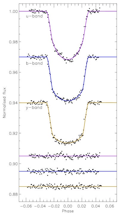
BUSCA is capable of viewing a transit simultaneously in four optical passbands, for which three passbands were chosen: Strömgren u, b & y. The fourth passband was neglected due to the need in using filters with the same optical depth. The only available filters with the same optical depth as the Strömgren filters were I-band filters (e.g., the Cousins I filter), however, these images were not used due to the target being saturated in the observed images. All four CCDs on BUSCA have a plate scale of 0.176 ′′pixel-1 and a field of view of ′, and were operated with binning. The instrument was defocussed and the telescope was autoguided throughout the observations. Due to the same transit being observed in a Cousins R filter on the CAHA 1.23 m it was decided to select filters to give observations in the optical UV–blue spectrum. With known difficulties in obtaining precise light curves in the optical UV from simultaneous multi-band photometry (e.g., Southworth et al., 2012, 2015b) the amount of defocusing used was calibrated in the Strömgren b passband, to optimise the precision of the light curves from all three Strömgren passbands. The resulting light curves (labelled U1, B1 and Y1) proved the strategy to be successful with all three light curves having an rms scatter of mmag per point (see Table 1). In particular the precision in the resulting u-band light curve is a major improvement (rms scatter: 1.08 mmag) on previous u-band light curves from simultaneous multi-band photometry (e.g., rms scatter: 3.46 mmag: Southworth et al. 2015b; 2.37 mmag: Mancini et al. 2013a; 3.55 mmag & 2.88 mmag: Ciceri et al. 2015).
2.2 CAHA 1.23 m telescope observations
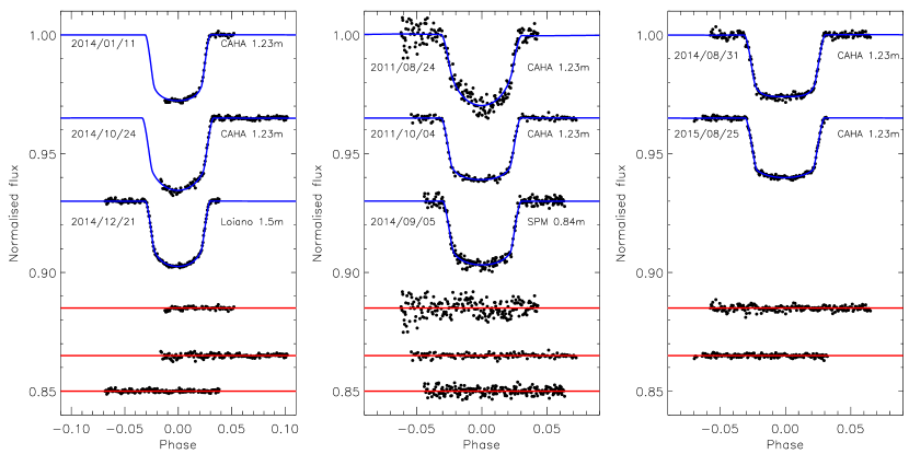
Six transits of the HAT-P-32 planetary system were observed using the CAHA 1.23 m telescope, Calar Alto, Spain. The CCD detector has a plate scale 0.32 ′′pixel-1 and a field of view of 21.5′21.5′. Two transits were observed using the Johnson V filter (V1: 2014/01/11 & V2: 2014/10/24), two in the Cousins R filter (R1: 2011/08/24 & R2: 2011/10/04) and two in the Cousins I filter (I1: 2014/08/31 & I2: 2015/08/25). All six transits were observed by defocusing the telescope and the telescope was autoguided throughout the observations. The two Johnson V transits were only partially covered, due to an ephemeris error (V1) and scheduling requirements (V2).
The transit I1 proved to be a poor fit. The initial modelling result disagreed with the 1- uncertainties from the other 10 transits (e.g., ). This anomalous result was duplicated when the transit was fitted using a second transit model: jktebop (see Southworth, 2008, for more details). Because the results from both models agreed within their 1- uncertainties, we concluded that the problem laid within the data itself. Therefore, we decided to only use this transit for the purpose of measuring the time of minimum light.
2.3 Cassini telescope observation
A transit of the HAT-P-32 planetary system was observed on 2014/12/21 using BFOSC on the Cassini 1.5 m telescope, Loiano Observatory, Italy, using a Johnson V filter (labelled V3). The BFOSC focal-reducing imager has a plate scale 0.58 ′′pixel-1. The telescope was defocused to allow exposure times of s and the pointing of the telescope was maintained throughout the night using the autoguider. The resulting light curve has the lowest rms scatter per point (0.55 mmag) of the transit light curves presented in this work.
2.4 San Pedro Mártir 0.84 m telescope observation
A transit of the HAT-P-32 planetary system was observed on 2014/09/05 using the San Pedro Mártir (SPM) 0.84 m telescope, Baja California, Mexico, using a Bessell R filter (labelled R3). The telescope was moderately defocused to allow exposure times of s and the pointing of the telescope was maintained throughout the night using the autoguider. The transit light curve was obtained as part of the The San Pedro Mártir Transit Observations Program (Ricci et al., 2015, 2017).
2.5 Aperture photometry
We reduced the data in an identical fashion to Southworth et al. (2009a, b, 2014). Aperture photometry was performed with an idl implementation of daophot (Stetson, 1987), and the aperture sizes were adjusted manually on a reference image to obtain the best rms scatter for the out-of-transit data (see Table 1). A first order polynomial was then fitted to the outside-transit data whilst simultaneously optimising the weights of the comparison stars. Both master bias, sky flat fields and dome flat fields frames were constructed. However, they were left out of the final data reduction as they had little effect on the final reduced science light curves. The resulting data have scatters ranging from 0.551 to 3.540 mmag per point versus a transit fit using prism. The timestamps from the fits files were converted to BJD/TDB. An observing log is given in Table 1.
3 Updates to PRISM & GEMC
The analysis of the transit light curves presented in this work was conducted by using prism (Planetary Retrospective Integrated Star-spot Model)555The latest versions of both prism and gemc are directly available from the author via email. alongside with the optimisation algorithm gemc (Genetic Evolution Markov Chain) (see Tregloan-Reed et al., 2013, 2015). The codes are written in idl666For further details see http://www.harrisgeospatial.com. (Interactive Data Language) and were developed to model the transit, limb darkening (LD) and starspots on the stellar disc simultaneously. The LD was implemented using the standard quadratic law. prism uses a pixellation approach to represent the star and planet on a two-dimensional array in Cartesian coordinates. Six parameters are used to model the transit: the ratio between the planetary and stellar radii, the sum of the fractional radii777Where the fractional stellar and planetary radii are defined as the absolute radii scaled by the semimajor axis ()., the linear and quadratic LD coefficients, the orbital inclination and the time of mid-transit. Then four parameters are used to model each starspot: the longitude and co-latitude of the centre of the starspot on the stellar surface, the angular size of the starspot and the starspot’s contrast (the ratio between the intensity () of the starspot and the surrounding photosphere, ).
gemc was created in conjunction to prism to improve the efficiency of finding a global solution in a complex multivariate parameter space compared to conventional MCMC algorithms (Tregloan-Reed et al., 2013, 2015). gemc is a hybrid between an MCMC and a genetic algorithm888A genetic algorithm mimics biological processes by spawning successive generations of solutions based on breeding and mutation operators from the previous generation. and is based on the Differential Evolution Markov Chain (DE-MC) put forward by Ter Braak (2006). During the ‘burn-in’ stage gemc runs chains in parallel and for every generation each chain is perturbed by a dimensional vector within the parameter search space, where is the number of parameters being fitted. The perturbation vector is orientated within the parameter space, so that the current generation’s best-fitting chain lies at the centre of the potential perturbation space. Once the ‘burn-in’ stage is complete and the position of the global solution has been found, gemc switches to a DE-MC algorithm to determine the parameter uncertainties (see Tregloan-Reed et al., 2015).
While none of the transit data presented in this work contain any starspot anomalies, so do not require the use of prism, prism was used to maintain homogeneity with the first author’s previous work (WASP-19: Tregloan-Reed et al. 2013; WASP-50: Tregloan-Reed & Southworth 2013; WASP-6: Tregloan-Reed et al. 2015).
To help facilitate this work, two modifications were made to prism to aid in the analysis of the HAT-P-32 planetary system light curves. To take into account the blended M-dwarf companion, HAT-P-32 B, a third light ratio parameter was added. A Gaussian prior is used in fitting the third light ratio, to limit the sampled solutions to a Gaussian probability distribution centred around a known flux ratio. The flux ratios used in this work and how they were calculated are given in Section 4.1.
The second modification was to add the ability to model and fit the detrending polynomial coefficients used in the detrending of transit data. This is achieved by calculating a new flux value for each model point (), by adding an order polynomial (evaluated at the model point) to the original flux () of the model point:
| (1) |
where is the selected pivot point, is the model points and is the corresponding order coefficient. For a data set which has already been detrended by an order polynomial, the optimal solutions for the detrending coefficients will be zero (e.g., ), and so, there will be no net change in flux (i.e., ).
4 Data analysis
| Date | Label | Filter | Radius | Sum of | Orbital Inclination | Transit epoch |
|---|---|---|---|---|---|---|
| ratio | fractional radii | (degrees) | (BJD/TDB) | |||
| 2011/08/24 | R1 | R | 0.1479 0.0031 | 0.1918 0.0070 | 89.25 1.37 | 2455798.60255 0.00051 |
| 2011/08/24 | U1 | u | 0.1505 0.0019 | 0.1931 0.0027 | 89.19 0.88 | 2455798.60246 0.00024 |
| 2011/08/24 | B1 | b | 0.1537 0.0015 | 0.1903 0.0024 | 88.81 0.83 | 2455798.60239 0.00020 |
| 2011/08/24 | Y1 | y | 0.1510 0.0013 | 0.1904 0.0025 | 88.32 0.86 | 2455798.60223 0.00020 |
| 2011/10/04 | R2 | R | 0.1512 0.0013 | 0.1906 0.0023 | 88.69 0.85 | 2455839.45261 0.00017 |
| 2014/01/11 | V1 | V | 0.1502 0.0014 | 0.1890∗ | 89.34 0.56 | 2456669.35548 0.00037 |
| 2014/08/31 | I1 | I | 0.1553 0.0017 | 0.2021 0.0034 | 86.55 1.10 | 2456901.55634 0.00016 |
| 2014/09/05 | R3 | R | 0.1529 0.0014 | 0.1877 0.0019 | 89.08 0.88 | 2456905.85649 0.00022 |
| 2014/10/24 | V2 | V | 0.1578 0.0012 | 0.1890∗ | 89.57 0.63 | 2456955.30654 0.00043 |
| 2014/12/21 | V3 | V | 0.1515 0.0008 | 0.1901 0.0004 | 88.94 0.43 | 2457013.35687 0.00008 |
| 2015/08/25 | I2 | I | 0.1512 0.0007 | 0.1892 0.0009 | 88.60 0.50 | 2457260.60777 0.00010 |
All 11 transits of HAT-P-32 were modelled using prism and gemc (see Table 2 & Figs. 1 & 2). This was accomplished by selecting a large parameter search space to allow the global best fit solution to be found. As discussed in Tregloan-Reed et al. (2013, 2015), the ability of gemc to find the global minimum in a short amount of computing time meant that it was possible to search a large area of the parameter space to avoid the possibility of missing the best solution. Both the third light ratio and the detrending polynomial coefficient were fitted during the modelling stage. Due to a first order polynomial being used to detrend the data, only a first order polynomial was used to model the data. From a previous study of HAT-P-32 it was confirmed that the planet followed a circular orbit (Zhao et al., 2014), therefore, the orbital eccentricity () and the argument of periastron () were set to zero and not fitted.
For the two incomplete transits V1 and V2 the sum of the fractional radii was fixed to the value found by Gibson et al. (2013): , this was done to maintain homogeneity with the results from the planetary radius variations (see Section 5), while, also agreeing within the 1- uncertainties with the remaining data sets.
4.1 Third light ratios
Due to the blended M-dwarf companion (HAT-P-32 B) within the HAT-P-32 defocussed PSF, the light ratio in the passbands in which the transits were observed needed to be found before the transits could be modelled. We used the light ratios determined by Zhao et al. (2014) in the and passbands. These passbands were selected as they give the largest wavelength range from all the possible measured light ratios in Zhao et al. (2014), thus improving the extrapolation to the passbands needed in this work. For the analysis we took the Strömgren filter profiles from the Calar Alto observatory999See https://www.caha.es/guijarro/BUSCA/caracter.html. The profiles from Bessell & Murphy (2012) were used for the V, R and I passbands as these are by design an approximation and improvement of the Johnson V, Cousins R and I filter profiles. From this analysis we determined the third light ratios (see Table 3) needed for the different passbands used to observe the transits in this work. All the light ratios are below the 1% flux contamination level. We then used the respective passband light ratios in prism and gemc to model (see Section 3) the 11 transits presented in this work.
| Passband | Third light ratio |
|---|---|
| Strömgren u | |
| Strömgren b | |
| Strömgren y | |
| Johnson V | |
| Cousins R | |
| Bessell R | |
| Cousins I |
4.2 Photometric results
The photometric parameters for the HAT-P-32 system are given in Table 2. The weighted means of the system parameters and with their 1- uncertainties together with their comparisons to published values are given in Table 4. The combined photometric results shows excellent agreement with previous published results. Fig. 1 & Fig. 2 compares the light curves to the best-fitting models, including the residuals.
| This | |||
|---|---|---|---|
| Work | 0.1515 0.0004 | 0.1902 0.0003 | 88.98 0.21 |
| H11 | 0.1508 0.0004 | 0.1902 0.0005∗ | 88.9 0.4 |
| S12 | 0.1531 0.0012 | 0.1928 0.0029∗ | 88.16 |
| G13 | 0.1515 0.0012 | 0.1890 0.0015∗ | 89.12 |
| S14 | 0.1510 0.0004 | 0.1901 0.0005∗ | 88.92 0.10 |
| M16 B | 0.1515 0.0012 | 0.1904 0.0030∗ | 88.61 0.84 |
| M16 R | 0.1505 0.0005 | 0.1903 0.0018∗ | 88.56 0.57 |
| N16 | 0.1516 | 0.1881 ∗ | 89.33 |
∗The sum of the fractional radii from the literature was calculated using the respective values for and .
References: (1) Hartman et al. (2011); (2) Sada et al. (2012); (3) Gibson et al. (2013); (4) Seeliger et al. (2014); (5) Mallonn & Strassmeier (2016); (6) Nortmann et al. (2016); (7) This Work
| Time of minimum | Cycle | Residual | Reference | |
|---|---|---|---|---|
| (BJD/TDB 2400000) | no. | (BJD) | ||
| 54420.44712 | 0.00009 | 0.0 | -0.00007 | 1 |
| 55798.60255 | 0.00051 | 641.0 | 0.00023 | 7 |
| 55798.60246 | 0.00024 | 641.0 | 0.00014 | 7 |
| 55798.60239 | 0.00020 | 641.0 | 0.00007 | 7 |
| 55798.60223 | 0.00020 | 641.0 | -0.00009 | 7 |
| 55839.45261 | 0.00017 | 660.0 | 0.00014 | 7 |
| 55843.75341 | 0.00019 | 662.0 | 0.00092 | 2 |
| 55845.90287 | 0.00024 | 663.0 | 0.00038 | 2 |
| 55845.90314 | 0.00040 | 663.0 | 0.00065 | 2 |
| 55867.40301 | 0.00073 | 673.0 | 0.00044 | 4 |
| 55880.30267 | 0.00033 | 679.0 | 0.00005 | 4 |
| 55895.35297 | 0.00016 | 686.0 | 0.00029 | 4 |
| 55895.35249 | 0.00080 | 686.0 | -0.00019 | 4 |
| 55897.50328 | 0.00033 | 687.0 | 0.00059 | 4 |
| 55910.40274 | 0.00043 | 693.0 | 0.00001 | 4 |
| 55923.30295 | 0.00031 | 699.0 | 0.00017 | 4 |
| 55942.65287 | 0.00064 | 708.0 | 0.00002 | 4 |
| 56155.50385 | 0.00026 | 807.0 | 0.00020 | 4 |
| 56157.65470 | 0.00072 | 808.0 | 0.00105 | 4 |
| 56177.00392 | 0.00025 | 817.0 | 0.00020 | 3 |
| 56183.45364 | 0.00085 | 820.0 | -0.00011 | 4 |
| 56183.45361 | 0.00049 | 820.0 | -0.00014 | 4 |
| 56185.60375 | 0.00033 | 821.0 | -0.00001 | 4 |
| 56185.60379 | 0.00011 | 821.0 | 0.00003 | 6 |
| 56211.40361 | 0.00056 | 833.0 | -0.00024 | 4 |
| 56220.00440 | 0.00019 | 837.0 | 0.00051 | 3 |
| 56245.80345 | 0.00007 | 849.0 | -0.00053 | 5 |
| 56254.40404 | 0.00022 | 853.0 | 0.00003 | 4 |
| 56542.50538 | 0.00032 | 987.0 | 0.00029 | 4 |
| 56542.50530 | 0.00018 | 987.0 | 0.00021 | 4 |
| 56542.50522 | 0.00052 | 987.0 | 0.00013 | 4 |
| 56572.60532 | 0.00018 | 1001.0 | 0.00012 | 4 |
| 56598.40539 | 0.00017 | 1013.0 | 0.00009 | 4 |
| 56600.55546 | 0.00017 | 1014.0 | 0.00016 | 4 |
| 56628.50585 | 0.00031 | 1027.0 | 0.00044 | 4 |
| 56656.45533 | 0.00045 | 1040.0 | -0.00018 | 4 |
| 56669.35548 | 0.00037 | 1046.0 | -0.00008 | 7 |
| 56901.55634 | 0.00016 | 1154.0 | -0.00008 | 7 |
| 56905.85649 | 0.00022 | 1156.0 | 0.00005 | 7 |
| 56955.30654 | 0.00043 | 1179.0 | -0.00008 | 7 |
| 57013.35687 | 0.00008 | 1206.0 | 0.00003 | 7 |
| 57260.60777 | 0.00010 | 1321.0 | 0.00001 | 7 |
The available times of mid-transit for HAT-P-32 were collected (see Table 5) from the literature (Hartman et al., 2011; Sada et al., 2012; Gibson et al., 2013; Seeliger et al., 2014; Mallonn & Strassmeier, 2016; Nortmann et al., 2016). The value used from Mallonn & Strassmeier (2016) was calculated as the weighted mean between the independently fitted blue and red values. All timings were converted to the BJD/TDB timescale and used to obtain an improved orbital ephemeris:
where represents the cycle count with respect to the reference epoch and the bracketed quantities represent the uncertainty in the final two digits of the preceding number. Fig. 3 and Table 5 show the residuals of these times against the ephemeris. The overall fit of the times of mid-transit are in agreement with a linear ephemeris by 1.6-, which, indicate that the results show no evidence for transit timing variations. When the two major outliers, at 7.6- (56245.80345: Mallonn & Strassmeier, 2016) and 4.9- (55843.75341: Sada et al., 2012), are removed from the analysis the overall fit improves to 0.9-.
The times of mid-transit from Seeliger et al. (2014) were taken from the 20 ‘good’ transits presented in their work. However, the transit they obtained on 2013/01/04 was not used in this analysis due to the reported mid-transit time not agreeing with the reported date.

4.3 Physical properties of the HAT-P-32 planetary system
| Parameter | This Work | H11 | ||
| () | 1.182 | 0.041 | 0.026 | 1.160 0.041 |
| () | 1.225 | 0.015 | 0.009 | 1.219 0.016 |
| (cgs) | 4.3349 | 0.0054 | 0.0032 | 4.33 0.01 |
| () | ||||
| () | 0.80 | 0.14 | 0.01 | 0.86 0.164 |
| () | 1.807 | 0.022 | 0.013 | 1.789 0.025 |
| ( m s-2) | 6.6 | |||
| () | 0.126 | 0.023 | 0.001 | 0.143 0.030 |
| (K) | 1786 26 | |||
| 0.0256 | 0.0046 | 0.0002 | 0.028 0.005 | |
| (AU) | 0.03448 | 0.00041 | 0.00025 | 0.0343 0.0004 |
| Age (Gyr) | 2.7 0.8 | |||
We used the same approach101010For a detailed discussion on the methodology used in the analysis see Southworth (2009). as described by Tregloan-Reed et al. (2015), in that we used the photometric properties of HAT-P-32 to determine the physical characteristics. The analysis used a set of parameters which were obtained from the analysed light curves and previously published spectra, plus tabulated predictions of theoretical models. We adopted the values of , and from Table 4, while, the orbital velocity amplitude m s-1, the stellar effective temperature K and metal abundance from Zhao et al. (2014).
The standard formulae and the physical constants listed by Southworth (2011) were used in conjunction with a starting value of , to calculate the physical properties of the system. The stellar expected and radius was determined through interpolating the mass and of the star within a set of tabulated predictions from theoretical stellar models. At each iteration was refined until the best agreement was found between the expected and observed , and the expected and measured . This was performed from the zero-age to the terminal-age main sequence, in steps of 0.01 Gyr. This approach then yielded the estimates of the system physical parameters and the evolutionary age of the star.
Due to the differing agreements and systematic errors between various theoretical stellar models, this methodology was repeated separately using five different sets of stellar theoretical models (see Southworth, 2010), and the Gaussian distribution of the parameter output values was used to determine the systematic error. A perturbation algorithm was then used to propagate the statistical errors (see Southworth, 2010).
The final results of this process are in agreement with themselves and are in excellent agreement with published results for HAT-P-32 (see Table 6). The final physical properties are given in Table 6 and contains the individual statistical and systematic errorbars for the parameters which have a dependency on the theoretical models. The largest of the five statistical errorbars from the five theoretical stellar models, is used for the final statistical errorbar, for each parameter. The same is true for the systematic errorbar which is calculated from the standard deviation (1-) of the parameter values.
5 Variation of planetary radius with wavelength
| Telescope / | Label | Passband | FWHM | ||||
|---|---|---|---|---|---|---|---|
| Instrument | (nm) | (nm) | () | ||||
| BUSCA | U1 | Strömgren u | 350 | 30 | 0.02513 0.00008 | 1.850 0.006 | 0.39 |
| BUSCA | B1 | Strömgren b | 467 | 18 | 0.02497 0.00007 | 1.838 0.005 | 0.35 |
| BUSCA | Y1 | Strömgren y | 547 | 23 | 0.02486 0.00007 | 1.830 0.005 | 0.36 |
| CAHA 1.23 m | V1 | Johnson V | 544.8 | 84 | 0.02496 0.00007 | 1.837 0.005 | 0.33 |
| CAHA 1.23 m | V2 | Johnson V | 544.8 | 84 | 0.02592 0.00009 | 1.908 0.007 | 0.43 |
| Cassini 1.5 m | V3 | Johnson V | 544.8 | 84 | 0.02489 0.00005 | 1.832 0.004 | 0.23 |
| CAHA 1.23 m | R1 | Cousins R | 640.7 | 158 | 0.02423 0.00041 | 1.784 0.030 | 1.96 |
| CAHA 1.23 m | R2 | Cousins R | 640.7 | 158 | 0.02468 0.00007 | 1.816 0.005 | 0.33 |
| SPM 0.84 m | R3 | Bessell R | 630 | 118 | 0.02506 0.00009 | 1.845 0.006 | 0.42 |
| CAHA 1.23 m | I2 | Cousins I | 798 | 154 | 0.02491 0.00006 | 1.834 0.004 | 0.27 |
The 11 datasets of the HAT-P-32 planetary system presented in this work were obtained using seven different passbands. One dataset was observed simultaneously in three-passbands (Strömgren u, b & y from BUSCA), and the other eight were observed using Johnson V, Bessell R, Cousins R and I passbands (from the CAHA 1.23 m, SPM 0.84 m and Cassini 1.5 m telescopes). Due to this, it is only natural to search for possible variations in the planetary radius in these passbands. For this we follow the same procedure of Southworth et al. (2015b), in that we refit the light curves with all the parameters fixed, except for , and the detrending polynomial coefficients. We keep fixed for the two incomplete transits (V1 and V2). As mentioned in Section 2.2 the I1 transit was not used in this analysis, so only ten datasets were used.
The fractional planetary radius, is represented in our modelling of the light curves by the parameter , which is directly linked to the primary observable: the transit depth. The parameter which is directly comparable to theoretical predictions is the absolute planetary radius (). In prism the fractional radii are used111111The fractional radii share a correlation with the other photometric parameters (see Southworth, 2008), so a transformation using the semimajor axis, is required to find from : . However, (and its associated uncertainty) is an absolute property of the system and therefore will be the same, irrespective of which passband is used to observe a transit. Refitting the light curves by using a fixed allows to find a set of values and uncertainties which are directly comparable to each other (see Table 7).
Our ten planetary radius measurements cover the optical wavelength range from 350 nm to 798 nm. In order to increase the scope of our analysis we include the results from Gibson et al. (2013) (520–930 nm). To obtain a direct comparison between the two sets of results, we fixed the fractional stellar radius and the orbital inclination to the values found by Gibson et al. (2013), when we refitted the light curves. This was made possible due to the fact that our results for these two parameters are in agreement to the values from Gibson et al. (2013) (see Table 4).
Figs. 4 and 5 show the transformed values as a function of the central wavelength of the passband from the analysis. The FWHM of each passband is shown as a horizontal line for reference. The fitted parameter and the passband characteristics are given in Table 7 together with the uncertainties in given in units of pressure scale height, . We calculated using the planetary equilibrium temperature, K (see Table 6) and found an agreement with the approximation ( km) given by Gibson et al. (2013), with km. The relative uncertainties for 90 % of our measured radii of HAT-P-32 A b are smaller than one atmospheric pressure scale height. This indicates that our measurements are sensitive to radius variations at the 1 level. Our data therefore, are in principle, sensitive to the properties of the atmosphere of HAT-P-32 A b.
By examining Table 7 it can be seen that the refitted planetary radius from dataset V2 is larger than expected (considering the values from the remaining Johnson V passbands). As this is one of the partial transits the anomalous result can be explained as an artefact from the data reduction stage. We therefore did not use the from this transit in the comparison to the theoretical model spectra. The transit observed with the Cousins R filter on the CAHA 1.23 m telescope, R1 appears to be shallower than expected. This smaller radius can be accounted for by the poor quality of the light curve, due to the contribution of systematics and the small amount of defocus used. We therefore used the weighted mean of , from the two observed transits in the Cousins R filter (R1 & R2) for our comparisons to the theoretical model spectra.
5.1 Theoretical transmission model spectra
We initially compared our planetary radius measurements to 15 theoretical transmission spectra which, were generated121212Three additional transmission spectra were generated as variations of a bimodal cloud particle distribution by altering different atmospheric model parameters. by the model atmosphere code of Mollière et al. (2015, 2017), seven of which are shown in Figs. 4 and 5. petitCODE (Mollière et al., 2015, 2017) is a model which calculates exoplanet atmospheric structures in radiative–convective equilibrium, including absorption and scattering processes, and the self–consistent treatment of clouds. As an output the code returns the planet’s emission and transmission spectra. For the model calculations presented here, a two–pronged approach for generating cloudy spectra was followed: (i) using the planet–star system parameters (host star temperature and radius, planet’s semi–major axis, radius and mass), and assuming a fiducial atmospheric enrichment of [Fe/H] = 0.55 we calculated self-consistent clear and cloudy structures and spectra for HAT-P-32 A b. For these calculations the cloud model parameter choice as defined in Mollière et al. (2017), Table 2, was used, while the atmospheric enrichment was chosen following the method described in Section 4.1 of Mollière et al. (2017). (ii) In addition to these spectra with a self–consistent cloud treatment we also considered the standard approach (see, e.g., Sing et al., 2016) to take our fiducial cloud-free atmospheric structure of this planet, and adding a grey cloud deck and/or a Rayleigh scattering haze, the latter of which was included by scaling the H2/He Rayleigh cross-sections by a given factor.
Cloud modelling following approach (i): in the self–consistent cloud calculations, the particle opacities for the clouds are determined from either Mie theory or the distribution of hollow spheres (DHS) approach (Min et al., 2005). Mie theory uses the classical assumption of spherically homogeneous grains. DHS uses a distribution of hollow spheres to determine the optical properties of irregularly shaped dust aggregates. The model assumes zero interaction between the different chemical species of clouds. The different species considered are MgAl2O4, Mg2SiO4, Fe, KCl and Na2S (Mollière et al., 2017).
The 15 theoretical transmission spectra generated and used in this work span a range of different atmospheric model parameters: metal enrichment, C/O number ratio, TiO/VO opacity, cloud particle settling parameter, cloud mass fractions, cloud deck pressures and Rayleigh haze scaling factors131313As written above, in the calculations in which the clouds are not included in a self-consistent fashion the use of a Rayleigh scattering haze does not stem from H2/He, however, it is how the haze is implemented: small particle clouds (i.e., hazes) with particle sizes smaller than the observation wavelength, lead to a Rayleigh scattering signal. But as the cloud species are unknown, the H2/He cross–sections are scaled, to mimic the haze.. The first theoretical transmission spectrum which was generated, represents a clear cloudless model using a scaled solar metal enrichment level combined with a solar C/O number ratio. TiO/VO opacity was not added. This spectrum can be considered as the ‘base’ spectrum in this work. Five more base transmission spectra were generated with the following variations: an order of magnitude increase and decrease in the metal enrichment (e.g., and ), and a doubling and halving of the C/O number ratio. TiO/VO opacity was added to the fifth base transmission spectrum.
Cloud opacity was added to a further six generated base transmission spectra. The cloud opacity was treated using the Self Consistent Coupling (SCC) method as described by Mollière et al. (2017). One of the cloud transmission spectra used the Ackerman & Marley (2001) (A01) cloud model to allow the coupling between the effects of clouds with the atmospheric temperature iteration. It should be noted that for this work the implementation of the Ackerman & Marley (2001) model differs from the original, by accounting for the vertical mixing induced by insolation and setting the radiative layer mixing length equal to the atmospheric pressure scale height (see Mollière et al., 2017). For this transmission spectrum DHS was used to describe the cloud particles with the cloud particle settling parameter set to: , which is the ratio between the mass averaged grain settling velocity and the atmospheric mixing velocity (Mollière et al., 2017). It was found by Mollière et al. (2017) that it is only possible to replicate a steep Rayleigh slope in the optical, if small cloud particles (0.06 to 0.12 m) are placed into the atmosphere at high layers. Therefore the other five base cloudy transmission spectra using the SCC method used a parametrised cloud model, corresponding to vertically homogeneous clouds, however, not larger than a given maximum value, which is a simple way of treating settling, and used a mono–disperse particle size of 0.08 m. The first spectrum used Mie theory (homogeneous spherical grains) to describe the cloud particles and used a parametrised cloud model with a maximum cloud mass fraction within the atmosphere set to: (where is the atmospheric metal mass fraction). Three spectra were generated using DHS to describe the cloud particles but each had a different maximum cloud mass fraction: , and . The final base cloudy transmission spectrum generated using the SCC method had a maximum cloud mass fraction of , however, Fe opacity was added to the clouds. This has the effect of dampening any Rayleigh scattering in the optical due to the strong absorbing nature of Fe in the optical (Mollière et al., 2017).
Cloud modelling following approach (ii): three theoretical transmission spectra were generated by using the cloudless self-consistent atmospheric structures, obtained as described above, and then adding cloud opacity only for the spectral calculations. The properties of the added cloud opacity are determined from the cloud pressure deck and a Rayleigh haze scaling factor. Each of the three transmission spectra had a metal enrichment level: combined with a solar C/O number ratio. One of the spectra had a cloud pressure deck set at 0.001 bar. For the second transmission spectrum a Rayleigh haze scaling factor of 100 was used with an omitted cloud pressure deck. The final transmission spectrum had both a 0.001 bar cloud pressure deck and an added Rayleigh haze scaling factor of 100.
5.2 Fitted theoretical transmission spectra results
We fitted the radial offset of each model spectrum to the planetary radius measurements via a MCMC algorithm and determined the reduced chi squared, between all the theoretical transmission spectra and the planetary radius measurements, whilst taking into account the FWHM of each passband.
| (2) |
where is the chi squared value, is the total number of data points, is the number of fitted model parameters, and so, is the number of degrees of freedom141414The number of degrees of freedom () used in this work was ..
| Model spectra | Best Fit | BUSCA agreement |
| Cloudless clear spectra | ||
| Base | 4.9 | 3.0 |
| TiO/VO | 21.6 | 7.3 |
| 4.5 | 3.9 | |
| 4.5 | 1.5 | |
| Twice solar C/O ratio | 5.6 | 2.8 |
| Half solar C/O ratio | 4.9 | 3.3 |
| SCC cloud spectra | ||
| A01 cloud model | 1.4 | 0.94 |
| Mie cloud particles† | 1.6 | 0.63 |
| DHS | 1.7 | 1.2 |
| DHS | 1.8 | 1.3 |
| DHS | 2.3 | 0.46 |
| DHS Fe clouds† | 2.1 | 1.4 |
| Added cloud opacity | ||
| Cloud only | 2.1 | 1.6 |
| Haze only | 2.2 | 1.2 |
| Cloud and haze | 1.4 | 0.19 |
The Mie and DHS Fe cloud models have an , see Table 2 Mollière et al. (2017). In addition, the DHS Fe clouds model also has all the other cloud species in it, but with the addition of Fe, while the nominal DHS/Mie- models have no Fe included.
The results from fitting the 15 theoretical transmission spectra to the planetary radius measurements are presented in Table 8.
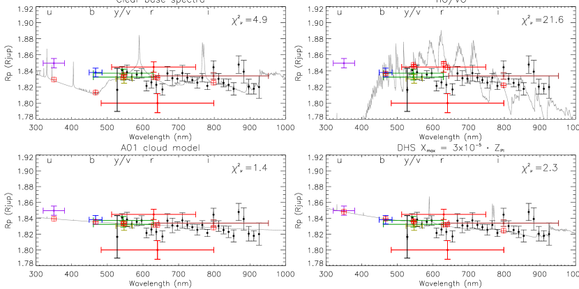
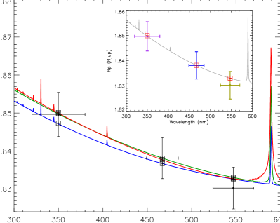
Fig. 4 shows the comparison between the best fit of four of the theoretical transmission spectra and the planetary radius measurements. The two upper panels of Fig. 4 show two of the clear cloudless transmission spectra: the base transmission spectrum and the transmission spectrum with added TiO/VO opacity. The two bottom panels of Fig. 4 show two of the cloud spectra which were generated using the SCC method: the A01 cloud model (Ackerman & Marley, 2001) and the cloud spectrum generated using DHS to describe the cloud particles and using a maximum cloud mass fraction, .
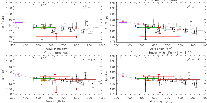
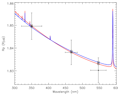
Fig. 5 shows the comparison between the best fit of four of the theoretical transmission spectra with added cloud opacity151515Three of these spectra can be found in Table 8. The bottom right panel of Fig. 5 shows a spectrum with an added bimodal cloud opacity generated, using an alternate set of parameters (see Section 5.3).; and with that of the planetary radius measurements. The two upper panels of Fig. 5 show two transmission spectra: a spectrum with an added cloud pressure deck set at 0.001 bar and the transmission spectrum with an added Rayleigh haze scaling factor of 100. The two bottom panels of Fig. 5 show two transmission spectra where a bimodal cloud opacity was added.
The best fitting theoretical transmission spectrum to the planetary radius measurements (in Table 8) is the base spectrum with clouds from the cloud approach (i), generated using the A01 cloud model (). Equally in agreement though, at , is the fitted spectrum generated with approach (ii), i.e., a model with a metal enrichment of , an added cloud opacity using a cloud pressure deck of 0.001 bar, and a Rayleigh haze scaling factor of 100. This confirms and agrees with previous studies (e.g., Gibson et al., 2013; Mallonn et al., 2016) in detecting a grey absorbing cloud deck within the atmosphere of HAT-P-32 A b. When the two best fitting spectra are examined (bottom left of Figs. 4 and 5), it is seen that both have the same agreement over the entire wavelength range (350 nm–798 nm) of radius measurements. However, when the two spectra are compared to the BUSCA data (350 nm–547 nm) alone, it can be clearly seen that the combined cloud deck and haze spectrum gives a superior agreement at: 0.19- compared with 0.94- for the A01 cloud model spectrum (see Table 8). The detection of a Rayleigh–like scattering haze between 350 nm–547 nm agrees with the previous study by Mallonn & Strassmeier (2016).
5.3 Theoretical transmission spectra with added bimodal cloud opacity
The ensemble of different wavelength dependent radii variations used in this work were observed independently on different nights, with the exception of the three BUSCA radius measurements. This leads to an addition of an unquantifiable uncertainty into the radius measurements due to temporal effects161616Such as stellar noise (e.g., un-occulted starspots) and different atmospheric observing conditions.. However, the BUSCA radius measurements were collected simultaneously and therefore are not affected by temporal effects. Examining the BUSCA radius measurements, we can see a linear negative gradient ( while ). This is indicative of a Rayleigh–like scattering slope. The theoretical transmission spectrum which was generated with the cloud modelling approach (ii) used a bimodal cloud particle distribution to simulate a cloud pressure deck (0.001 bar) combined with a joint Rayleigh haze (scaling factor 100). The base spectra using the A0 cloud model did not exhibit a behaviour equivalent to a Rayleigh–like scattering haze, due to large cloud particle sizes and added Fe droplets (see Mollière et al., 2017). This explains how the two best fitting transmission spectra disagree below 550 nm. The bimodal cloud particle distribution transmission spectrum gives a superior agreement to the BUSCA radius measurements171717Note the agreement between the BUSCA radius measurements and the transmission spectra, was determined after the spectrum was fitted to the entirety of the radius measurements in this work. Including the data points from Gibson et al. (2013).. When taking into account that the BUSCA measured radii are free from temporal uncertainties, there is a greater likelihood that the bimodal cloud particle distribution transmission spectrum is the correct interpretation of the data.
To explore the bimodal cloud particle distribution solution further we looked into variations between the grey cloud deck pressure and the haze scaling factor. To see if it is possible to reproduce such an excellent agreement with the BUSCA radius measurements (e.g., 0.5-), whilst still achieving a good fit (e.g., ) with the entirety of the radius measurements used in this work. Increasing the cloud deck pressure will result in different temperatures being probed during the transmission observation, because the atmospheric temperature is a function of pressure. Moreover, atomic and molecular lines will gain in importance in the spectrum when compared to the cloud opacity, making, e.g., the alkali Na and K lines very strong in the spectral range studied here. However, this can be circumvented by altering the metal enrichment: by rescaling the temperature structure to lower pressures for higher metal enrichment or higher pressures for lower metal enrichment (Mollière et al., 2015).
To show this, we took our clear base transmission spectra, one with an increase and the other with a decrease by an order of magnitude in the metal enrichment (e.g., and ). Cloud opacity was added to each of the transmission spectra. A cloud pressure deck of 0.01 bar and a lower Rayleigh haze scaling of 10 were used as proxies for the cloud properties for the transmission spectrum with . A cloud pressure deck of 0.0001 bar and a higher Rayleigh haze scaling of 1000 were used for the transmission spectrum with . The two transmission spectra were then fitted to the planetary radius measurements as described in Section 5.2. The best fit for the high and low pressure transmission spectra was found to be and respectively. The low pressure transmission spectrum with is shown in the lower right panel of Fig. 5. The agreement between the two new bimodal cloud particle distribution transmission spectra and the BUSCA radius measurements was 0.21- (0.01 bar) and 0.37- (0.0001 bar). Fig. 6 shows the comparison between the three bimodal transmission spectra and the three radius measurements from BUSCA. Fig. 6 shows how it is not possible to discern the difference between the three bimodal cloud particle distributions, when using the BUSCA data alone. This can be explained due to a degeneracy between the cloud pressure deck and Rayleigh haze scaling factor. In the case of a much lower metal enrichment then the importance of the molecules with respect to Rayleigh scattering would go down. Therefore a lower value of the Rayleigh haze scaling factor would be needed to yield a strong Rayleigh scattering slope when compared to the molecular features. The BUSCA planetary radius measurements do though, constrain the ratio between the strength of the grey absorbing cloud deck relative to the haze component.
The results from comparing the three bimodal cloud particle distribution transmission spectra with the planetary radius measurements used in this work show that varying the strengths of the cloud pressure deck and the Rayleigh haze scaling factor has little effect on the final fit or the agreement between the transmission spectra and with that of the BUSCA radius measurements. While in essence the three bimodal cloud particle distribution spectra are variations of the same solution, their unison good fit to the planetary radius measurements combined with their excellent agreement to the BUSCA radius measurements, adds considerable weight to a bimodal cloud particle distribution solution instead of a unimodal cloud particle distribution. A bimodal cloud particle distribution solution would also explain the discrepancies in the results found from previous studies which detected either a grey absorbing cloud deck or a Rayleigh–like scattering haze.
To study the structure of a bimodal cloud particle distribution we looked into two different scenarios: A Rayleigh–like haze stacked above a grey absorbing cloud deck181818This is the bimodal cloud particle distribution transmission spectrum using a metal enrichment , Rayleigh haze scaling factor and 0.001 bar cloud pressure (see Table 8 and Figs. 5 and 6)., or a Rayleigh–like haze and a grey absorbing cloud which are homogeneously extended throughout the atmosphere. To ascertain which scenario best agreed with the planetary radius measurements in this work we generated a new transmission spectrum using approach (ii). Both the cloud and haze particles were set at the same altitude to create a bimodal cloud particle distribution. In this scenario, at the shortest wavelengths the Rayleigh–like scattering would overpower the grey absorbing clouds due to its wavelength dependence () while at longer wavelengths the grey absorbing clouds overcome the Rayleigh–like scattering. To better understand this one can use a variation of Eq. 1 from Lecavelier Des Etangs et al. (2008).
| (3) |
where is the planetary radius at the evaluated wavelength , is the base planetary radius, is the atmospheric scale height and is the wavelength dependent opacity.
In the two different scenarios is determined differently. When the grey absorbing cloud particles are homogeneously extended throughout the atmosphere, can be calculated as follows:
| (4) |
where and are the opacities for the Rayleigh haze and grey cloud deck respectively, is a reference wavelength point, and is the wavelength at which is being evaluated.
Eq. 4 shows that while is constant at all wavelengths, is dependent on wavelength. This allows a homogeneously extended Rayleigh–like haze and grey absorbing cloud to produce both a Rayleigh–like scattering slope at short wavelengths and a flat grey absorption at longer wavelengths.
For the new transmission spectrum we introduced a grey absorber with an opacity of 0.01 cm2 g-1, instead of using a cloud pressure deck. The grey absorber was spread homogeneously throughout the entire atmosphere. We then fitted the transmission spectrum to the planetary radius measurements and obtained for the best fit. This is in equal agreement to the Rayleigh–like haze stacked over a grey absorbing cloud deck (see Table 8). The new homogeneous grey absorber transmission spectrum agrees with the three BUSCA radius measurements at 0.27-. Fig. 7 shows the comparisons between the two bimodal cloud particle distributions; the stacked spectrum and the homogeneous grey absorber spectrum and with that of the three BUSCA radius measurements. From examining Fig. 7 it can be seen that with the current data at hand, it is not possible to discern between the two bimodal scenarios. We calculated that a 15-fold increase in the precision of the planetary radii measurements, would be needed to allow for a distinction between the two bimodal scenarios. Combined with this, both transmission spectra equally agree with the entirety of the radius measurements in this work. Therefore it is not possible to describe the cloud / haze properties any further, other than to mention the existence of a bimodal cloud particle distribution within the atmosphere of HAT-P-32 A b. However, it should be noted that cloud particles large enough to generate a grey cloud opacity would tend to settle more strongly, potentially generating a thick cloud deck below the smaller haze particles, due to the smaller ratio between the surface area and mass of the larger cloud particles.
6 Discussion and conclusions
HAT-P-32 A b is an inflated, low density hot-Jupiter planet orbiting a hot ( K) host star, which makes the planet a perfect candidate to perform studies of planetary atmospheres. We used the collected data to determine the physical properties of the HAT-P-32 planetary system (Table 6) based on 11 new high-precision transit light curves and finding values which are consistent with those in the literature. We find the mass and radius of the host star to be and , respectively. For the planet we find a mass of , a radius of and a density of .
The 11 transits of HAT-P-32 were modelled using prism and gemc. This included two incomplete transits (observed in the Johnson V passband), for which we fixed, the sum of the fractional radii to the value determined by Gibson et al. (2013). This is due to the sum of the fractional radii being directly related to the transit duration. It was set to the value from Gibson et al. (2013) to maintain homogeneity with the second analysis into the variations of with wavelength. This though, did not help with the partial transit observed on 2014/10/24. All of the parameter best fits from the partial transit observed on 2014/01/11 and the full transit observed in the Johnson V passband agree within their 1- uncertainties. While, for the partial transit observed on the 2014/10/24 this is not the case for , which disagrees with the other two Johnson V light curves by , however, the remaining parameters do agree within the 1- uncertainties.
We observed one of the transits of HAT-P-32 using a simultaneous multi-band imaging instrument: BUSCA (using the Strömgren u, b and y passbands). Due to the known difficulty in attempting to obtain a high-precision light curve in the optical–UV via this technique, it was decided to select three passbands close to the UV-blue side of the optical spectrum. In conjunction with this we optimised the amount of defocusing used in the Strömgren b passband to maximise the precision of the light curves in all three passbands. The resulting light curves produced are of decent quality (1 mmag scatter per point). In terms of the optical UV we were able to obtain a light curve with a rms scatter 1.08 mmag per point. Our new u-band light curve has a threefold increase in precision compared to previous optical–UV light curves obtained using BUSCA (i.e., Southworth et al., 2015b). This has allowed an accurate measurement of the planetary radius in the optical–UV which is important for detecting either a Rayleigh scattering slope or the blue-edge detection of TiO in the planetary atmosphere.
Taking into account a blended M-dwarf companion (HAT-P-32 B) within the defocused PSF of HAT-P-32 A, combined with needing to study variations in the planetary radius with respect to wavelength, modifications were made to the modelling and optimisation codes prism and gemc. After making the new modifications, prism and gemc were then used in the analysis of the 11 transit in this work. The new versions are available from the first author.
6.1 Rayleigh–like haze and grey absorbing cloud deck
The results from comparing the different planetary radii from each passband to the individual theoretical model atmospheres, confirms the results from Gibson et al. (2013); Mallonn et al. (2016) by the detection of a grey absorbing cloud deck within the upper atmosphere of HAT-P-32 A b. The planetary radius measurements from each passband were compared to the cloudy spectra, generated using a bimodal cloud particle distribution which consisted of a Rayleigh haze combined with a grey absorbing cloud pressure deck, showed the same level of agreement and confirms the possible presence of a Rayleigh haze within the atmosphere of HAT-P-32 A b as found by Mallonn & Strassmeier (2016). However, the bimodal cloud particle distribution spectra give a superior agreement to the three radius measurements obtained from the BUSCA observations using the Strömgren u, b and y passbands. Considering that the BUSCA radius measurements were the only observations obtained simultaneously in this study – and therefore are not affected by unquantifiable temporal uncertainties – allows for a greater weight to be placed on the accuracy of the set, compared to the remaining radius measurements individually. A similar argument can be used to explain the discrepancy between Mallonn & Strassmeier (2016) and Mallonn et al. (2016). Mallonn & Strassmeier (2016) used transit spectroscopy where the observations were simultaneously obtained, while, Mallonn et al. (2016) used an ensemble of photometric transit observations spanning from 2007 to 2016.
At present there is supporting evidence for the presence of a Rayleigh scattering haze in the upper atmosphere of HAT-P-32 A b from a prior investigation. Mallonn & Strassmeier (2016) performed transit spectroscopy to observe a transit of HAT-P-32 A b. The data agreed with a Rayleigh scattering model in the optical–UV, with greater clarity below 550 nm. However, a second study using photometric observations by Mallonn et al. (2016) seemed to contradict the original results. Mallonn et al. (2016) mentions a discrepancy between the two data sets in the redder wavelengths and attributed this to systematics in the measurement from Mallonn & Strassmeier (2016). The new data presented by Mallonn et al. (2016) showed equal weight towards either a Rayleigh scattering model or that of a flat cloudy spectrum. When the data from both studies were combined and examined with a restricted wavelength range of nm, the results showed a strong agreement with a flat cloudy spectrum. The Rayleigh scattering transmission spectrum which was generated by the model from Fortney et al. (2010) which was used in Mallonn & Strassmeier (2016); Mallonn et al. (2016) gives a continuous gradient from 350 nm to 950 nm. However, in other cases where a Rayleigh scattering slope has been found, it is generally detected below 550 nm (e.g., WASP-12 b: Sing et al., 2013). When examining the combined data from both Mallonn & Strassmeier (2016) and Mallonn et al. (2016) it can be seen that the data could support a bimodal cloud particle distribution transmission spectrum approach, and so, support the detection of a Rayleigh–like scattering haze.
There have been previous exoplanet studies into the variation of the planetary transit depth at various wavelengths in the optical–UV photometric bands (e.g., Turner et al., 2013, 2016). In an attempt to measure the magnetic field of TrES-3 b Turner et al. (2013), obtained nine transits, four of which was observed using a Bessell U filter between June 2009 and April 2012. When examining the transit depths they determined a non-detectable change in the planetary radius between the Bessell U and Harris V filters. However, the major difference between the optical-UV transits in this work compared to the optical-UV transits from Turner et al. (2013), is that for this work the three BUSCA transits were observed simultaneously and have an average rms scatter of 1 mmag. While, the Bessell U transits from Turner et al. (2013) where each taken on different nights (introducing temporal uncertainties) and are of poorer quality, with a rms scatter of 4.1 mmag for the four combined phased Besselll U transits. Therefore, masking any spectral features or changes between the near–UV bands.
Turner et al. (2016) recently completed an observational survey of 15 exoplanets, collecting photometric light curves in the optical-UV (Bessell-U, Harris-B, V and R). The overall results showed a non-detectable change in the planetary radius between the optical and near–UV, for 10 of the exoplanets, while, the other five exoplanets results; indicate the presence of an aerosol / Rayleigh scattering process. This survey supports the case that a scattering slope in the optical–UV is detectable using ground-based photometry.
Gibson et al. (2013) performed transit spectroscopy to observe the atmosphere of HAT-P-32 A b191919The results of their analysis are included in this work. using GMOS on the Gemini North telescope. Through their analysis they determined that a grey absorber (cloud) was masking spectral features. A Rayleigh scattering slope is most prominent below 550 nm, which lies beyond of the observing range of Gibson et al. (2013) (520–930 nm). In this analysis it was found that the data from Gibson et al. (2013) agreed with the A0 cloudy (Ackerman & Marley, 2001) transmission spectrum () and the bimodal cloud particle distribution spectrum (). Therefore, we confirm that a grey absorber / cloud deck is present within the atmosphere of HAT-P-32 A b.
The variations between the observed planetary radius with wavelength due to Rayleigh scattering is dependent on a power-law relation between wavelength and the mean cross-section of the atmospheric scattering particles (Lecavelier Des Etangs et al., 2008). The power-law coefficient which corresponds to Rayleigh scattering is (Lecavelier Des Etangs et al., 2008). To ascertain the validity of the Rayleigh scattering slope detection we fitted a straight line to the Strömgren u, b and y radii against wavelength and determined the gradient . We then calculate the temperature of the planet’s terminator , due to the slope of the planetary transmission spectrum being proportional to :
| (5) |
where is the mean molecular weight, which is taken as , is the surface gravity and being the Boltzmann constant.
By assuming that the gradient is induced by Rayleigh scattering and therefore setting , gives a temperature for the terminator of K, which fits (within the 1- uncertainty) with the equilibrium temperature, K (see Table 6) and is still below the day-side temperature of K (see Zhao et al., 2014). Though it is not in agreement with the value found by Mallonn & Strassmeier (2016) ( K), however, Mallonn & Strassmeier (2016) states that their value appears to underestimate the true temperature of the terminator.
As a second validation check, the slope of the planetary transmission spectrum can be used to calculate the planetary mass and the result then compared to our previous result (see Table 6). For this we use the MassSpec concept by de Wit & Seager (2013). Because the pressure scale height is dependent on the surface gravity and therefore the planetary mass, while, also being dependent on the power-law relation between wavelength and the mean cross-section of the atmospheric scattering particles, we can use our derived gradient to calculate the planetary mass using the following equation (see Southworth et al., 2015a, and references therein):
| (6) |
where is the gravitational constant.
We applied MassSpec to our determined gradient and by assuming , we find a planetary mass of for HAT-P-32 A b. This is in good agreement to the value found from analysing the transit light curves ( ).
Recently Batalha et al. (2017) has called in question the use of MassSpec for determining the mass of small planets (), due to the uncertainty in different types of dominant atmospheres (e.g., CH4 or CO2), and so, it is not possible to assume a value for . This therefore, makes the use of MassSpec difficult for use in determining the mass of small planets, with a range of different molecular constituents. As HAT-P-32 A b is a hot Jupiter planet then the concerns of using MassSpec brought up by Batalha et al. (2017) have no implications in this work.
The results from this work show a possible detection of a bimodal cloud particle distribution () within an atmosphere comprising of a scaled solar metal enrichment and a solar C/O number ratio for HAT-P-32 A b. The results from this work help towards confirming the tentative findings from Mallonn & Strassmeier (2016). The gradient of the Rayleigh–like haze scattering slope provides an extra validation by allowing the determination of the temperature at the terminator (1518345 K) and the planetary mass (0.940.16 ), which, are confirmed through the separate analysis of the transit light curves. By obtaining high-precision ( 1 mmag) transit light curves in the optical-UV, this work shows that these measurements are important in the detection of either a Rayleigh scattering haze or a rich TiO atmosphere from ground based simultaneous multi-band photometry.
7 Acknowledgements
We would like to thank the anonymous referee for their helpful comments and in particular their comments regarding the descriptions of the theoretical transmission spectra used in this work. This paper incorporates observations collected at the Centro Astronómico Hispano Alemán (CAHA) at Calar Alto, Spain, operated jointly by the Max-Planck Institut für Astronomie and the Instituto de Astrofísica de Andalucía (CSIC). Together with observations collected at the Observatorio Astronómico Nacional at San Pedro Mártir. JTR acknowledges financial support from USRA (Universities Space Research Association), ORAU (Oak Ridge Associated Universities) and NASA in the form of a Post-Doctoral Programme (NPP) Fellowship. DR acknowledges financial support from the Spanish Ministry of Economy and Competitiveness (MINECO) under the 2011 Severo Ochoa Program MINECO SEV-2011-0187.
The following internet-based resources were used in the research for this paper: the NASA Astrophysics Data System; the SIMBAD database and VizieR catalogue access tool operated at CDS, Strasbourg, France; and the ariv scientific paper preprint service operated by Cornell University.
References
- Ackerman & Marley (2001) Ackerman, A. S., Marley, M. S., 2001, ApJ, 556, 872
- Adams et al. (2012) Adams, E. R., Ciardi, D. R., Dupree, A. K., Gautier, III, T. N., Kulesa, C., McCarthy, D., 2012, AJ, 144, 42
- Adams et al. (2013) Adams, E. R., Dupree, A. K., Kulesa, C., McCarthy, D., 2013, AJ, 146, 9
- Baglin et al. (2006) Baglin, A., et al., 2006, in 36th COSPAR Scientific Assembly, vol. 36 of COSPAR Meeting, p. 3749
- Bakos et al. (2004) Bakos, G., Noyes, R. W., Kovács, G., Stanek, K. Z., Sasselov, D. D., Domsa, I., 2004, The Publications of the Astronomical Society of the Pacific, 116, 266
- Batalha et al. (2017) Batalha, N. E., Kempton, E. M.-R., Mbarek, R., 2017, ApJL, 836, L5
- Bessell & Murphy (2012) Bessell, M., Murphy, S., 2012, PASP, 124, 140
- Borucki et al. (2010) Borucki, W. J., et al., 2010, Science, 327, 977
- Burrows et al. (2010) Burrows, A., Rauscher, E., Spiegel, D. S., Menou, K., 2010, ApJ, 719, 341
- Butler et al. (1996) Butler, R. P., Marcy, G. W., Williams, E., McCarthy, C., Dosanjh, P., Vogt, S. S., 1996, The Publications of the Astronomical Society of the Pacific, 108, 500
- Butler et al. (1999) Butler, R. P., Marcy, G. W., Fischer, D. A., Brown, T. M., Contos, A. R., Korzennik, S. G., Nisenson, P., Noyes, R. W., 1999, ApJ, 526, 916
- Charbonneau et al. (2002) Charbonneau, D., Brown, T. M., Noyes, R. W., Gilliland, R. L., 2002, ApJ, 568, 377
- Chen et al. (2014) Chen, G., et al., 2014, A&A, 563, A40
- Ciceri et al. (2015) Ciceri, S., et al., 2015, A&A, 577, A54
- de Wit & Seager (2013) de Wit, J., Seager, S., 2013, Science, 342, 1473
- Dragomir et al. (2015) Dragomir, D., Benneke, B., Pearson, K. A., Crossfield, I. J. M., Eastman, J., Barman, T., Biddle, L. I., 2015, ApJ, 814, 102
- Dressing et al. (2014) Dressing, C. D., Adams, E. R., Dupree, A. K., Kulesa, C., McCarthy, D., 2014, AJ, 148, 78
- Fischer et al. (2016) Fischer, P. D., et al., 2016, ApJ, 827, 19
- Fortney (2005) Fortney, J. J., 2005, MNRAS, 364, 649
- Fortney et al. (2008) Fortney, J. J., Lodders, K., Marley, M. S., Freedman, R. S., 2008, ApJ, 678, 1419
- Fortney et al. (2010) Fortney, J. J., Shabram, M., Showman, A. P., Lian, Y., Freedman, R. S., Marley, M. S., Lewis, N. K., 2010, ApJ, 709, 1396
- Gibson et al. (2013) Gibson, N. P., Aigrain, S., Barstow, J. K., Evans, T. M., Fletcher, L. N., Irwin, P. G. J., 2013, MNRAS, 436, 2974
- Greiner et al. (2008) Greiner, J., et al., 2008, PASP, 120, 405
- Hartman et al. (2011) Hartman, J. D., et al., 2011, ApJ, 742, 59
- Hellier et al. (2011) Hellier, C., Anderson, D. R., Collier-Cameron, A., Miller, G. R. M., Queloz, D., Smalley, B., Southworth, J., Triaud, A. H. M. J., 2011, ApJ, 730, L31
- Hubeny et al. (2003) Hubeny, I., Burrows, A., Sudarsky, D., 2003, ApJ, 594, 1011
- Irwin et al. (2008) Irwin, P. G. J., et al., 2008, Journal of Quantitative Spectroscopy & Radiative Transfer, 109, 1136
- Latham (1992) Latham, D. W., 1992, in McAlister, H. A., Hartkopf, W. I., eds., IAU Colloq. 135: Complementary Approaches to Double and Multiple Star Research, vol. 32 of Astronomical Society of the Pacific Conference Series, p. 110
- Lecavelier Des Etangs et al. (2008) Lecavelier Des Etangs, A., Pont, F., Vidal-Madjar, A., Sing, D., 2008, A&A, 481, L83
- Madhusudhan & Seager (2009) Madhusudhan, N., Seager, S., 2009, ApJ, 707, 24
- Mallonn & Strassmeier (2016) Mallonn, M., Strassmeier, K. G., 2016, A&A, 590, A100
- Mallonn et al. (2016) Mallonn, M., et al., 2016, MNRAS, 463, 604
- Mancini et al. (2016) Mancini, L., Giordano, M., Mollière, P., Southworth, J., Brahm, R., Ciceri, S., Henning, T., 2016, MNRAS, 461, 1053
- Mancini et al. (2013a) Mancini, L., et al., 2013a, A&A, 551, A11
- Mancini et al. (2013b) Mancini, L., et al., 2013b, MNRAS, 430, 2932
- Mancini et al. (2013c) Mancini, L., et al., 2013c, MNRAS, 436, 2
- Mancini et al. (2014) Mancini, L., et al., 2014, MNRAS, 443, 2391
- Min et al. (2005) Min, M., Hovenier, J. W., de Koter, A., 2005, A&A, 432, 909
- Mollière et al. (2015) Mollière, P., van Boekel, R., Dullemond, C., Henning, T., Mordasini, C., 2015, ApJ, 813, 47
- Mollière et al. (2017) Mollière, P., van Boekel, R., Bouwman, J., Henning, T., Lagage, P.-O., Min, M., 2017, A&A, 600, A10
- Neuhäuser et al. (2011) Neuhäuser, R., et al., 2011, Astronomische Nachrichten, 332, 547
- Nikolov et al. (2013) Nikolov, N., Chen, G., Fortney, J. J., Mancini, L., Southworth, J., van Boekel, R., Henning, T., 2013, A&A, 553, A26
- Nikolov et al. (2016) Nikolov, N., Sing, D. K., Gibson, N. P., Fortney, J. J., Evans, T. M., Barstow, J. K., Kataria, T., Wilson, P. A., 2016, ApJ, 832, 191
- Nikolov et al. (2014) Nikolov, N., et al., 2014, MNRAS, 437, 46
- Nikolov et al. (2015) Nikolov, N., et al., 2015, MNRAS, 447, 463
- Nortmann et al. (2016) Nortmann, L., Pallé, E., Murgas, F., Dreizler, S., Iro, N., Cabrera-Lavers, A., 2016, A&A, 594, A65
- Pollacco et al. (2006) Pollacco, D. L., et al., 2006, The Publications of the Astronomical Society of the Pacific, 118, 1407
- Queloz et al. (2000) Queloz, D., et al., 2000, A&A, 354, 99
- Ricci et al. (2015) Ricci, D., et al., 2015, PASP, 127, 143
- Ricci et al. (2017) Ricci, D., et al., 2017, PASP, 129, 064401
- Ricker et al. (2009) Ricker, G. R., et al., 2009, in American Astronomical Society Meeting Abstracts #213, vol. 41 of Bulletin of the American Astronomical Society, p. 193
- Sada et al. (2012) Sada, P. V., et al., 2012, PASP, 124, 212
- Schneider et al. (2011) Schneider, J., Dedieu, C., Le Sidaner, P., Savalle, R., Zolotukhin, I., 2011, A&A, 532, A79
- Seager & Sasselov (2000) Seager, S., Sasselov, D. D., 2000, ApJ, 537, 916
- Seeliger et al. (2014) Seeliger, M., et al., 2014, MNRAS, 441, 304
- Sing et al. (2011) Sing, D. K., et al., 2011, MNRAS, 416, 1443
- Sing et al. (2013) Sing, D. K., et al., 2013, MNRAS, 436, 2956
- Sing et al. (2015) Sing, D. K., et al., 2015, MNRAS, 446, 2428
- Sing et al. (2016) Sing, D. K., et al., 2016, Nature, 529, 59
- Southworth (2008) Southworth, J., 2008, MNRAS, 386, 1644
- Southworth (2009) Southworth, J., 2009, MNRAS, 394, 272
- Southworth (2010) Southworth, J., 2010, MNRAS, 408, 1689
- Southworth (2011) Southworth, J., 2011, MNRAS, 417, 2166
- Southworth et al. (2012) Southworth, J., Mancini, L., Maxted, P. F. L., Bruni, I., Tregloan-Reed, J., Barbieri, M., Ruocco, N., Wheatley, P. J., 2012, MNRAS, 422, 3099
- Southworth et al. (2009a) Southworth, J., et al., 2009a, MNRAS, 396, 1023
- Southworth et al. (2009b) Southworth, J., et al., 2009b, MNRAS, 399, 287
- Southworth et al. (2014) Southworth, J., et al., 2014, MNRAS, 444, 776
- Southworth et al. (2015a) Southworth, J., et al., 2015a, MNRAS, 447, 711
- Southworth et al. (2015b) Southworth, J., et al., 2015b, MNRAS, 454, 3094
- Stetson (1987) Stetson, P. B., 1987, PASP, 99, 191
- Sudarsky et al. (2003) Sudarsky, D., Burrows, A., Hubeny, I., 2003, ApJ, 588, 1121
- Ter Braak (2006) Ter Braak, C. J. F., 2006, Statistics and Computing, 16, 239
- Tregloan-Reed & Southworth (2013) Tregloan-Reed, J., Southworth, J., 2013, MNRAS, 431, 966
- Tregloan-Reed et al. (2013) Tregloan-Reed, J., Southworth, J., Tappert, C., 2013, MNRAS, 428, 3671
- Tregloan-Reed et al. (2015) Tregloan-Reed, J., et al., 2015, MNRAS, 450, 1760
- Turner et al. (2013) Turner, J. D., et al., 2013, MNRAS, 428, 678
- Turner et al. (2016) Turner, J. D., et al., 2016, MNRAS, 459, 789
- Wheatley et al. (2013) Wheatley, P. J., et al., 2013, in European Physical Journal Web of Conferences, vol. 47 of European Physical Journal Web of Conferences, p. 13002
- Zhao et al. (2014) Zhao, M., et al., 2014, ApJ, 796, 115