Inverse problem for the Helmholtz equation with Cauchy data: reconstruction with conditional well-posedness driven iterative regularization

Abstract

In this paper, we study the performance of Full Waveform Inversion (FWI) from time-harmonic Cauchy data via conditional well-posedness driven iterative regularization. The Cauchy data can be obtained with dual sensors measuring the pressure and the normal velocity. We define a novel misfit functional which, adapted to the Cauchy data, allows the independent location of experimental and computational sources. The conditional well-posedness is obtained for a hierarchy of subspaces in which the inverse problem with partial data is Lipschitz stable. Here, these subspaces yield piecewise linear representations of the wave speed on given domain partitions. Domain partitions can be adaptively obtained through segmentation of the gradient. The domain partitions can be taken as a coarsening of an unstructured tetrahedral mesh associated with a finite element discretization of the Helmholtz equation. We illustrate the effectiveness of the iterative regularization through computational experiments with data in dimension three. In comparison with earlier work, the Cauchy data do not suffer from eigenfrequencies in the configurations.

1 Introduction

Iterative methods for the recovery of subsurface parameters have been collectively referred to, in reflection seismology, as Full Waveform Inversion (FWI). FWI consists in the minimization of the residuals, defined as some difference between the observed and modelled data. FWI was originally formulated with time-domain data using an energy norm in the misfit functional by Lailly [23] and Tarantola [38, 39]. The time-harmonic formulation of the seismic inverse problem was later considered by Pratt et al. [33, 32]. Standardly, one applies the adjoint state method for the implementation of the minimization procedure.

To mitigate the nonlinearity and ill-posedness of the inverse problem, hierarchical multiscale strategies have been developed. In the time-domain, Bunks et al. [11] proposed successive inversion of data subsets of increasing frequency contents. This multiscale approach can be related to the subspace search method introduced in [21]. Multiscale Gauss-Newton-Krylov methods were developed by Akcelik et al. [2] and many further developments have taken place since then. The application of wavelet bases enabling successive levels of model compression were considered by Loris et al. [27, 26] in wave-equation tomography and in FWI by Lin et al. in [25], Yuan and Simons in [43, 44]. These ideas were natural but lacked foundation and understanding of convergence. In [18], the authors developed an iterative regularization approach with a multilevel strategy derived from conditional Lipschitz stability estimates with a convergence analysis. For the regularization they introduced a multiscale hierarchy of subspaces for which the Lipschitz stability estimates hold, with an associated model compression rate through projections. This compression rate appears in the convergence analysis and mitigates the growth of stability constants with scale refinement, that is, increasing dimension of the subspaces. In the time-harmonic case, such quantitative stability estimates have been proved for piecewise constant [7] and piecewise linear [3] representations of the wave speed with a given domain partition; we refer to [3] for more extended bibliography. Note that, in view of recent work by Cârstea et al. [14], on a germane problem in elasticity, it seems quite possible to recover the partition as well, in the case where the domain is composed of sub-analytic sets. In the piecewise constant case, this includes subspaces defined by Haar wavelets, where the analysis in [3] is adapted to general domain partitions such as unstructured tetrahedral meshes, that can be associated with a segmentation. Here, we present a computational framework of our reconstruction algorithm via iterative regularization using piecewise linear representations as stable subspaces, as well as experiments.

We use Cauchy data assimilated from dual sensor acquisition. Cauchy data do not suffer from eigenfrequencies unlike the Dirichlet-to-Neumann map, which, in fact, cannot be observed directly in seismic marine acquisition. For a perspective on dual sensor acquisition devices and simultaneous measurements of pressure and vertical or normal velocity, we refer to [13, 40]. Dual sensor acquisition has additional benefits such as in noise reduction [41, 34]. Independent of earlier analysis, the results presented here confirm the relevance of acquiring dual sensor data. The marine seismic acquisition we consider consists in sources positioned above the fixed receivers lattice. This setup matches the TopSeis acquisition system that has been recently deployed by CGG (Compagnie Générale de Géophysique) and Lundin Norway AS, for the purpose of improving the near offset data.

The formulation of FWI, and its underlying minimization procedure, has been proposed with norms different from energy norms. Shin and collaborators [37, 6, 36] compared the use of the phase and/or amplitude information in the data. Envelope based misfit functional is considered in [8, 42]. Brossier, Operto and Virieux investigate the use of the $L^{1}$ norm in [9], and in combination with $L^{2}$ norm in [10]. In this paper, we introduce a new misfit functional which is based upon conditional stability of the inverse problem for Cauchy data. This functional, related to the Green’s identity, is formulated in terms of repeated integration of a quadratic expression. Such a formulation overcomes the difficulties of computational complexity occurring in discretizing operator norms, or distances of subspaces (which are typically used in theoretical stability estimates, [4, 3]). Further, it allows independent locations for field and computational sources in the discrete settings.

The paper is organized as follows. We detail the inverse problem and the main stability results in Section 2, where the misfit functional to minimize for the reconstruction procedure is given. In Subsection 2.4 the computation of the gradient of the misfit functional is conducted using the Lagrangian approach. In Section 3, numerical experiments are presented to demonstrate the efficiency of the algorithm, using single-frequency Cauchy data. Finally, Section 4 shows an experiment with different locations of observational and computational sources.

2 Misfit functional and stability result

2.1 Assumptions about the domain $\Omega$

We fix some notations that will be adopted in this paper. Given a point $x\in\mathbb{R}^{3}$, with $x=(x^{\prime},x_{3})$, where $x^{\prime}\in\mathbb{R}^{2}$ and $x_{3}\in\mathbb{R}$, $B_{r}(x),B_{r}^{\prime}(x^{\prime})$ denote the open balls in $\mathbb{R}^{3},\mathbb{R}^{2}$ centred at $x$, $x^{\prime}$ respectively with radius $r$. We also denote by $Q_{r}(x)$ the cylinder

$$Q_{r}(x)=B_{r}^{\prime}(x^{\prime})\times(x_{3}-r,x_{3}+r)$$

and $B_{r}=B_{r}(0)$ and $Q_{r}=Q_{r}(0)$.

1. We assume that $\Omega$ is a domain in $\mathbb{R}^{3}$ and that there exist positive constants $r_{0}$ and $B$ ($r_{0}$ being dimensionally a length, $B$ being an absolute constant), such that

   (2.1) $$|\Omega|\leq Br_{0}^{3},$$

   where $|\Omega|$ denotes the Lebesgue measure of $\Omega$.

2. We fix an open non-empty subset $\Sigma$ of $\partial\Omega$ (where the measurements in terms of the local Cauchy data are taken).

3. We assume that $\Omega$ can be decomposed as follows:

   $$\bar{\Omega}=\bigcup_{j=1}^{N}\bar{D}_{j},$$

   where $D_{j}$, $j=1,\dots,N$ are known open sets of $\mathbb{R}^{3}$, satisfying the conditions below.

   1. $D_{j}$, $j=1,\dots,N$ are connected and pairwise non-overlapping polyhedrons.

   2. $\partial{D}_{j}$, $j=1,\dots,N$ are of Lipschitz class with constants $r_{0}$, $L$ see, for example, [1]).

   3. There exists one region, say $D_{1}$, such that $\partial{D}_{1}\cap\Sigma$ contains a flat portion $\Sigma_{1}$ of size $r_{0}$ and for every $j\in\{2,\dots,N\}$, we can select a subchain $\{D_{j_{k}}\}_{k=1}^{K}$ ($K\leq N$) of the partition $\{D_{j}\}_{j=1}^{N}$ of $\Omega$, such that

      (2.2) $$D_{j_{1}}=D_{1},\qquad D_{j_{K}}={D_{j}}.$$

      In addition, for every $k=1,\dots,K$, ${D}_{j_{k-1}}$ and ${D}_{j_{k}}$ are contiguous in the sense that $\partial{D}_{j_{k}}\cap\partial{D}_{j_{k-1}}$ contains a flat portion $\Sigma_{k}$ of size $r_{0}$ (here we agree that $D_{j_{0}}=\mathbb{R}^{3}\setminus\Omega$), such that

      $$\Sigma_{k}\subset\Omega,\quad\mbox{for\>every}\>k=2,\dots,K.$$

      We illustrate the configuration and selection of subchain in Figure 1. We emphasize that under such an assumption, for every $k=1,\dots,K$, there exists $P_{k}\in\Sigma_{k}$ and a rigid transformation of coordinates (depending on $k$) under which we have $P_{k}=0$ and

      $$\Sigma_{k}\cap{Q}_{r_{0}/3} = \{x\in Q_{r_{0}/3}\>|\>x_{3}=0\},$$

      $$D_{j_{k}}\cap{Q}_{r_{0}/3} = \{x\in Q_{r_{0}/3}\>|\>x_{3}>0\},$$

      (2.3) $$D_{j_{k-1}}\cap{Q}_{r_{0}/3} = \{x\in Q_{r_{0}/3}\>|\>x_{3}<0\}.$$

(a) Domain decomposition, the ordering is arbitrary, at the exception of $D_{1}$ which is connected to $\Sigma$.

(b) Path towards the selected subdomain, e.g. $D_{j_{4}}$. $K=4$ in this illustration.

Figure 1: Illustration of the domain decomposition and the path towards a selected subdomain $D_{j_{k}}$.

2.2 A-priori information on the wave speed $c$

We shall consider a real valued function $c\in L^{\infty}(\Omega)$, with

(2.4) $$0<c_{min}\leq c\leq c_{max},$$

for some positive constants $c_{min},\>c_{max}$ and of type

(2.5a) $$c(x)=\sum_{j=1}^{N}c_{j}(x)\chi_{D_{j}}(x),\qquad x\in\Omega,$$

(2.5b) $$c_{j}(x)=a_{j}+A_{j}\cdot x,$$

where $a_{j}\in\mathbb{R}$, $A_{j}\in\mathbb{R}^{3}$ are scalar and vector valued constants respectively, and $\{D_{j}\}_{j=1}^{N}$, $j=1,\dots,N$ is the given partition of $\Omega$ introduced in Subsection 2.1.

2.3 Cauchy data and misfit functional

We let $\Omega$ denote the subsurface domain with Lipschitz boundary $\partial\Omega$ and $\Sigma$ the non-empty open portion of $\partial\Omega$ introduced in Subsection 2.1 where the acquisition is carried out. We introduce the subspace of $H^{1/2}(\partial\Omega)$,

$$H^{1/2}_{co}(\Sigma)=\{f\in H^{1/2}(\partial\Omega)\>|\>\operatorname{supp}\,f\subset\Sigma\}.$$

Its closure with respect to the $H^{1/2}(\partial\Omega)$ norm is the space $H^{1/2}_{00}(\Sigma)$. In a similar manner, we define $H^{1/2}_{00}(\partial\Omega\setminus\overline{\Sigma})$. We denote the pressure by $u$. The Cauchy data associated to $c$ is the space $\mathcal{C}^{\Sigma}_{c}$,

$$\mathcal{C}^{\Sigma}_{c}=\Big{\{}(f,g)\in H^{1/2}(\partial\Omega)|_{\Sigma}\times H^{-1/2}(\partial\Omega)|_{\Sigma} \big{|} \>\exists u\in H^{1}(\Omega)\ \text{weak solution to}\ \Delta u+k^{2}c^{-2}u=0\ \text{in}\ \Omega,$$

$$u\Big{|}_{\Sigma}=f,$$

$$\langle\frac{\partial u}{\partial\nu}\Big{|}_{\partial\Omega},\varphi\rangle=\langle g,\varphi\rangle,\ \forall\varphi\in H^{1/2}_{00}(\Sigma)\Big{\}}.$$

Here, $\langle\psi,\varphi\rangle$ denotes the duality between the complex valued spaces $H^{-\frac{1}{2}}(\partial\Omega)$, $H^{\frac{1}{2}}(\partial\Omega)$ based on the $L^{2}$ inner product

$$\langle\psi,\varphi\rangle=\int_{\partial\Omega}\psi\overline{\varphi}$$

and $H^{\frac{1}{2}}(\partial\Omega)\big{|}_{\Sigma}$ and $H^{-\frac{1}{2}}(\partial\Omega)\big{|}_{\Sigma}$ denote the restrictions of $H^{\frac{1}{2}}(\partial\Omega)$ and $H^{-\frac{1}{2}}(\partial\Omega)$ to $\Sigma$ respectively. $\mathcal{C}^{\Sigma}_{c}$ is a subspace of the Hilbert space $H^{\frac{1}{2}}(\partial\Omega)\big{|}_{\Sigma}\times H^{-\frac{1}{2}}(\partial\Omega)\big{|}_{\Sigma}$.

We embed $\Omega$ in an ambient domain $\Upsilon\supset\Omega$ as we will find convenient to introduce Green’s function not precisely for the physical domain $\Omega$ but for this augmented domain $\Upsilon$.

We recall that by assumption 3(c) of Subsection 2.1 we can assume that there exists a point $P_{1}$ such that up to a rigid transformation of coordinates we have that $P_{1}=0$ and (3c) holds with $\Sigma=\Sigma_{1}$. Denoting by

$$D_{0}=\left\{x\in(\mathbb{R}^{3}\setminus\Omega)\cap B_{\frac{r_{0}}{3}}\>\bigg{|}\>|x_{i}|<\frac{r_{0}}{6},\>i=1,2\>;\>-\frac{r_{0}}{6}<x_{3}<0\right\},$$

it turns out that the augmented domain $\Upsilon=\accentset{\circ}{\overline{(\Omega\cup D_{0})}}$ is of Lipschitz class with constants $\frac{r_{0}}{3}$ and $\widetilde{L}$, where $\widetilde{L}$ depends on $L$ only. Given $r>0$, we set

(2.6) $$\Gamma_{1}=\left\{x\in\Upsilon\ \bigg{|}\>|x_{i}|<\frac{r_{0}}{6},\ i=1,\ 2\ ;\ x_{3}=-\frac{r_{0}}{6}\right\},$$

(2.7) $$\Gamma_{2}=\partial\Upsilon\setminus\overline{\Gamma}_{1},$$

(2.8) $$(\Upsilon)_{r}=\left\{x\in\Upsilon\ \bigg{|}\ \mbox{dist}(x,\partial\Upsilon)>r\right\}.$$

We also introduce the following sets

(2.9) $$D^{{}^{\prime}}_{0}=\left\{x\in D_{0}\>\bigg{|}\>-\frac{r_{0}}{12}<x_{3}<0\right\},$$

(2.10) $$D^{{}^{\prime\prime}}_{0}=\left\{x\in D_{0}\>\bigg{|}\>-\frac{r_{0}}{6}<x_{3}<-\frac{r_{0}}{12}\right\},$$

(2.11) $$K_{0}=\left\{x\in D^{{}^{\prime\prime}}_{0}\>\bigg{|}\>|x_{i}|<\frac{r_{0}}{24},\>i=1,2\>;\>-\frac{13}{96}r_{0}<x_{3}<-\frac{11}{96}r_{0}\right\},$$

(2.12) $$K_{1}=\left\{x\in D^{{}^{\prime\prime}}_{0}\>\bigg{|}\>|x_{i}|<\frac{r_{0}}{12},\>i=1,2\>;\>-\frac{7}{48}r_{0}<x_{3}<-\frac{5}{48}r_{0}\right\},$$

(2.13) $$\Omega^{\prime}=\accentset{\circ}{\overline{(D^{{}^{\prime}}_{0}\cup\Omega)}}.$$

Note that, fixing the origin at the center of $D^{{}^{\prime\prime}}_{0},K_{0},K_{1}$ are concentric parallelograms scaled by the factors $\frac{1}{4},\frac{1}{2}$ respectively. We illustrate the geometry in Figure 2. Note also that this precise choice of scale parameters is just made for the sake of definiteness. What really matters is the general geometrical configuration, in particular we must have

$$\mbox{dist}(D^{{}^{\prime\prime}}_{0},\overline{\Omega})\geq\frac{r_{0}}{12}>0\quad\textnormal{and}\quad K_{0}\subset\subset K_{1}\subset\subset D^{{}^{\prime\prime}}_{0}.$$

We shall denote by $\Gamma(x,y)$ the standard fundamental solution to the Laplace equation which is

(2.14) $$\Gamma(x,y)=\frac{1}{4\pi|x-y|}\ .$$

(a) Two-dimensional positioning of the sets $D_{0}^{\prime}$ and $D_{0}^{\prime\prime}$ with respect to the domain $\Omega$.

(b) Three-dimensional representation of the sets given by (2.9)–(2.12), these are symmetric with respect to the $(x_{3},x_{1})$ plane.

Figure 2: Illustration of the sets that are defined in (2.9)–(2.12).

Definition 1.

Let $B$, $N$, $r_{0}$, $L$, $c_{min}$ and $c_{max}$ be given positive numbers with $N\in\mathbb{N}$. We will refer to this set of numbers as to the a-priori data. Several constants depending on the a-priori data will appear within the paper. In order to simplify our notation, any quantity denoted by $C,C_{1},C_{2},\dots$ will be called a constant understanding in most cases that it only depends on the a-priori data.

Next we introduce a mixed boundary value problem for $\Delta+k^{2}c^{-2}$ in $\Upsilon$ which is always well posed, independently of any a-priori condition on $c$, besides the assumption of being real valued and bounded. This shall enable us to construct Green’s function for $\Delta+k^{2}c^{-2}$ in $\Upsilon$.

We assume that the uppermost part $D_{0}$ of the domain $\Upsilon$ represents a region filled by water. The wave speed in $D_{0}$ can then be assumed to be known and constant with

(2.15) $$c=c_{0},\quad\text{in $D_{0}$.}$$

Pressure sources (air gun) are excited to produce impulses located at points in $K_{1}\subset D_{0}$ and Cauchy data are collected through dual sensors located at the surface $\Sigma$, which lies below $K_{1}$.

Pressure is assumed to be zero at the sea level $\Gamma_{1}$ (i.e., free surface), and to satisfy, on the remaining part of the boundary $\Gamma_{2}$ (of the region of interest), a (conventional) absorbing condition. If we model this problem in the frequency domain, and assume that the source is modeled by a Dirac’s delta concentrated at a point $y$, the pressure is represented as the Green’s function of the following mixed boundary value problem,

(2.16) $$\left\{\begin{array}[]{lcl}\Delta G_{c}(\cdot,y)+k^{2}c^{-2}(\cdot)G_{c}(\cdot,y)=-\delta(\cdot-y)\ ,&&\mbox{in $\Upsilon$ ,}\\ G_{c}(\cdot,y)=0\ ,&&\mbox{on $\Gamma_{1}$ ,}\\ \partial_{\nu}{G_{c}}(\cdot,y)-ik_{0}G_{c}(\cdot,y)=0\ ,&&\mbox{on $\Gamma_{2}$ .}\end{array}\right.$$

The theory developed, for example, in [12] shows that such a function $G_{c}$ exists and is unique in the case of constant wave speed $c$. Note that the term $k_{0}$ is conventionally assumed to be constant and known. The next theorem collects the main features of the Green’s function solving (2.16) also in the case of variable wave speed $c(x)$. A similar result, but with stronger hypothesis, was proven in [3, Propositions 3.1, 3.4, 3.5]. The thesis here is slightly weaker, but the argument is somewhat simpler.

Theorem 1.

For any $y\in\Upsilon$, there exists a unique distributional solution $G_{c}(\cdot,y)$ to (2.16). Moreover, there exists a constant $C>0$ depending on $r_{0},L,k$ and on $c_{min}$ such that for any $x,y\in{(\Upsilon)}_{r_{0}}$, $x\neq y$ we have that

(2.17) $$|G_{c}(x,y)-\Gamma(x,y)|\leq C\$$

and

(2.18) $$|{\nabla}_{y}G_{c}(x,y)-{\nabla}_{y}\Gamma(x,y)|\leq C(\big{|}\log|x-y|\big{|}+1)\ .$$

Moreover, let $Q_{k+1}$ be a point such that $Q_{k+1}\in B_{\frac{r_{0}}{8}}(P_{k+1})\cap\Sigma_{k+1}$ with $k\in\{1,\dots,N-1\}$, then the following inequality holds true for every $x\in B_{\frac{r_{0}}{16}}(P_{k+1})\cap D_{j_{k}+1}$ and every $y=Q_{k+1}-re_{3}$, where $r\in(0,\frac{r_{0}}{16})$

(2.19) $$|{\nabla}^{2}_{y}(G_{c}(x,y)-\Gamma(x,y))|\leq Cr^{-1}.$$

Here ${\nabla}^{2}_{y}$ denotes the Hessian matrix.

Proof.

Let $y\in\Upsilon$ and let $G_{0}$ be the Green’s function for the Laplace operator which solves

(2.20) $$\left\{\begin{array}[]{lcl}\Delta G_{0}(\cdot,y)=-\delta(\cdot-y)\ ,&&\mbox{in $\Upsilon$ ,}\\ G_{0}(\cdot,y)=0\ ,&&\mbox{on $\Gamma_{1}$ ,}\\ \partial_{\nu}{G_{0}}(\cdot,y)-ik_{0}G_{0}(\cdot,y)=0\ ,&&\mbox{on $\Gamma_{2}$ .}\end{array}\right.$$

The existence and uniqueness of a distributional solution $G_{0}\in L^{1}(\Upsilon)$ to (2.20) is a consequence of standard theory on boundary value problems for the Laplace equation. By standard techniques it can be proved that for any $y\in\Upsilon$ such that $\mbox{dist}(y,\partial\Upsilon)\geq\frac{r_{0}}{4}$ we have that $G_{0}(\cdot,y)\in L^{2}(\Upsilon)$. Now we define $R_{c}(\cdot,y)\in H^{1}(\Upsilon)$ to be the solution to

(2.21) $$\left\{\begin{array}[]{lcl}\Delta R_{c}(\cdot,y)+k^{2}c^{-2}R_{c}(\cdot,y)=-k^{2}c^{-2}G_{0}(\cdot,y)\ ,&&\mbox{in $\Upsilon$ ,}\\ R_{c}(\cdot,y)=0\ ,&&\mbox{on $\Gamma_{1}$ ,}\\ \partial_{\nu}{R_{c}}(\cdot,y)-ik_{0}R_{c}(\cdot,y)=0\ ,&&\mbox{on $\Gamma_{2}$ .}\end{array}\right.$$

The existence and uniqueness for (2.21) follows along the lines of the proof of [3, Proposition 3.1], which relies on the Fredholm altenative theory. Moreover, by arguments based on well-known estimates for the Cauchy problem contained in [3, Proposition 3.1], we have that

(2.22) $$\|R_{c}(\cdot,y)\|_{H^{1}(\Upsilon)}\leq C\|G_{0}(\cdot,y)\|_{L^{2}(\Upsilon)}$$

and, by standard interior estimates, that

(2.23) $$|R_{c}(x,y)|\leq C,$$

for any $x\neq y,\ x\in\Upsilon$ and $\mbox{dist}(y,\partial\Upsilon)\geq\frac{r_{0}}{4}$. If we form

(2.24) $$G_{c}(x,y)=G_{0}(x,y)+R_{c}(x,y),$$

then we end up with the following estimate

(2.25) $$|G_{c}(x,y)|\leq C|x-y|^{-1},$$

for any $x,y\in\Upsilon,\ x\neq y$ and $\mbox{dist}(x,\partial\Upsilon)\geq\frac{r_{0}}{4},\>\mbox{dist}(y,\partial\Upsilon)\geq\frac{r_{0}}{4}$ . The latter combined with the arguments in the proofs of [3, Propositions 3.4, 3.5] suffices to deduce (2.17), (2.18) and (2.19). ∎

Assuming that, for sources placed at arbitrary points $z\in K_{1}$, we can measure associated Cauchy data on $\Sigma$:

(2.26) $$G_{obs}(x,z),~{}\dfrac{\partial}{\partial\nu_{x}}G_{obs}(x,z),\quad x\in\Sigma,$$

we seek $c$ which minimizes the following misfit functional

(2.27) $$\mathcal{J}(c)=\int_{K_{1}\times K_{1}}\left|\int_{\Sigma}\left(G_{c}(x,y)\>\partial_{\nu}G_{obs}(x,z)-G_{obs}(x,z)\>\partial_{\nu}G_{c}(x,y)\right)\mathrm{d}\mu(x)\right|^{2}\>\mathrm{d}y\>\mathrm{d}z,$$

where $\mu$ denotes the element of surface measure.

The introduction of the misfit functional (2.27) is motivated by the following argument. Given two wave speeds $c^{(i)}$, $i=1,2$, consider the Green’s functions $G_{i}$, introduced in Theorem 1, corresponding to $c^{(i)}$ in $\Upsilon$ and the following quantity

(2.28) $$\mathcal{J}(c^{(1)},c^{(2)})=\int_{K_{1}\times K_{1}}\left|\mathcal{S}_{\mathcal{U}_{0}}(y,z)\right|^{2}\mathrm{d}y\>\mathrm{d}z,$$

where

(2.29) $$\mathcal{S}_{\mathcal{U}_{0}}(y,z)=\int_{\Sigma_{1}}\left(G_{1}(x,y)\>\partial_{\nu}G_{2}(x,z)-G_{2}(x,z)\>\partial_{\nu}G_{1}(x,y)\right)\mathrm{d}\mu(x),\quad\mbox{for\>any}\>y,z\in D_{0}.$$

Expressions of the form above have appeared in many occasions in the treatment of inverse boundary problems. Analogies can be found with the probe method by Ikehata [20], see also [31]. In particular, a very strong relation can be observed with the so-called reciprocity gap functional introduced by Colton and Haddar [17] for inverse scattering.

It would be a matter of an exercise to show that, fixing $y\in K_{1}$,

(2.30) $$c\in L^{\infty}(\Upsilon)\rightarrow\big{(}G_{c}(x,y)|_{\Sigma},~{}\partial_{\nu}G_{c}(x,y)|_{\Sigma}\big{)}\in H^{1/2}(\partial\Omega)|_{\Sigma}\times H^{-1/2}(\partial\Omega)|_{\Sigma}$$

is Fréchet differentiable. Note also that, since we are assuming (2.5a) and (2.5b) (that is, $c$ lives in a finite dimensional space), the $L^{\infty}(\Upsilon)$ norm can equivalently be replaced by the $L^{2}(\Upsilon)$ norm. This will enable us to apply to $\mathcal{J}$ a projected steepest descent method in Section 3.

Theorem 2.

Let $\Omega$, $D_{j}$, $j=1,\dots,N$ and $\Sigma$ be a domain, $N$ subdomains of $\Omega$ and a portion of $\partial\Omega$ as in section 2.1 respectively. Let $c^{(i)}$, $i=1,2$ be two wave speeds satisfying (2.4) and of type

(2.31) $$c^{(i)}=\sum_{j=1}^{N}c^{(i)}_{j}(x)\chi_{D_{j}}(x),\qquad x\in\Omega,$$

where

$$c^{(i)}_{j}(x)=a^{(i)}_{j}+A^{(i)}_{j}\cdot x,$$

with $a^{(i)}_{j}\in\mathbb{R}$ and $A^{(i)}_{j}\in\mathbb{R}^{3}$, then we have

(2.32) $$||c^{(1)}-c^{(2)}||_{L^{\infty}(\Omega)}\leq C\left(\mathcal{J}(c^{(1)},c^{(2)})\right)^{1/2},$$

where $C$ is a positive constant that depends on the a-priori data only.

Remark 1.

Note that the introduction of the misfit functional is driven on the one hand by our computational experiments and on the other hand, it is inspired by the method of singular solutions used in previous stability results (see [3] for the case of the Helmholtz equation). Although a natural metric on the space of Cauchy data $\mathcal{C}_{c}^{\Sigma}$ is given by the distance (aperture) $d$ introduced in [3, (2.8)], we have

(2.33) $$\mathcal{J}(c^{(1)},c^{(2)})\leq Cd(\mathcal{C}^{\Sigma}_{c^{(1)}},\mathcal{C}^{\Sigma}_{c^{(2)}})^{2}$$

and also

(2.34) $$\mathcal{J}(c^{(1)},c^{(2)})\leq C||\Lambda^{\Sigma}_{c^{(1)}}-\Lambda^{\Sigma}_{c^{(2)}}||_{*}^{2},$$

where $\Lambda^{\Sigma}_{c}:u\in H^{1/2}(\partial\Omega)|_{\Sigma}\rightarrow\partial_{\nu}u\in H^{-1/2}(\partial\Omega)|_{\Sigma}$ is the local Dirichlet-to-Neumann map with its natural norm (here denoted by $||\cdot||_{*}$) between local trace spaces. These estimates justify the use of $\mathcal{J}$ as a substitute to the more traditional quantifications of the error on boundary data (either involving distance of spaces of Cauchy data or boundary maps).

Proof.

of Theorem 2.

The proof requires only some adaptations of [3, Theorem 2.2], which are outlined below.

i)

We introduce different boundary conditions. This aspect involves some modifications in the constructions of the Green’s function and has been treated in Theorem $1$ above. Note that we took advantage of the fact that here we focus on the three-dimensional case only.

ii)

We replace the domain $\Omega$ with $\Omega^{\prime}$ and add as initial subdomain $D_{0}^{\prime}$ instead of $D_{1}$. We take advantage of the fact that $c^{(1)}=c^{(2)}=1$ in $D_{0}^{\prime}\subset\Upsilon\setminus\overline{\Omega}$ which allows us to skip the arguments of [3, Section 4.3].

iii)

We observe that in [3, Theorem 2.2] the right-hand side in formula $(2.20)$ is expressed in terms of the distance between spaces of Cauchy data. However, the only Cauchy data that are actually used are those arising from Green’s function with pole in $\widehat{D}_{0}$. And the role of $\widehat{D}_{0}$ (see [3]) can be equivalently taken by the set $K_{0}$ introduced here in (2.11). Moreover, such Cauchy data intervene only in expressions like the one in (2.29) above. Therefore, the right-hand side of [3, (2.20)] can be replaced by

(2.35) $$\sup_{K_{0}\times K_{0}}|S_{\mathcal{U}_{0}}(y,z)|.$$

We also recall that $S_{\mathcal{U}_{0}}(y,z)$ is a solution to

(2.36) $$(\Delta_{y}+\Delta_{z}+2k^{2})S_{\mathcal{U}_{0}}(y,z)=0$$

in $D_{0}\times D_{0}$ (see [3, (4.61)]). Consequently, by standard estimate of boundedness in the interior we have

(2.37) $$\sup_{K_{0}\times K_{0}}|S_{\mathcal{U}_{0}}(y,z)|^{2}\leq C\int_{K_{1}\times K_{1}}|S_{\mathcal{U}_{0}}(y,z)|^{2}\>\mathrm{d}y\>\mathrm{d}z$$

where $C>0$ is a constant depending on $k$ and on $r_{0}$ .

iv)

Another difference comes from the fact that we are now assuming $c^{(i)}$ piecewise linear instead of $q^{(i)}=k^{2}(c^{(i)})^{-2}$, for $i=1,2$. However due to the assumption (2.4) the estimation of $c^{(i)},\nabla c^{(i)}$ at each interface is equivalent to that for $q^{(i)},\nabla q^{(i)}$, for $i=1,2$.

∎

The stability given in Theorem 2 justifies the use of (2.27) for an optimization algorithm toward the inversion of Cauchy data to wave speed.

2.4 Computation of the gradient using the adjoint state method

We start by observing that, although $c\rightarrow G_{c}(x,y)$ does not map into $H^{1}(\Upsilon)$ (because of the singularity of the Green’s function), the derivative $D_{c}G_{c}(x,y)[c]\delta c$ exists and does belong in $H^{1}(\Upsilon)$. This can be achieved by recalling (2.21) and (2.24). That is

(2.38) $$R_{c}(x,y)=G_{c}(x,y)-G_{0}(x,y)\quad\in H^{1}(\Upsilon),$$

and the second term $G_{0}$ is independent of $c$. Hence we may well define

(2.39) $$D_{c}G_{c}(x,y)[c]\delta c=D_{c}R_{c}(x,y)[c]\delta c.$$

We denote

(2.40) $$H_{\Gamma_{1}}^{1}(\Upsilon)=\{v\in H^{1}(\Upsilon)~{}|~{}v|_{\Gamma_{1}}=0\}.$$

We continue with the variational formulation of Problem (2.16). As noted above, denoting $R_{c}(x,y)=G_{c}(x,y)-G_{0}(x,y)$, it can be formulated as

(2.41) $$\int_{\Upsilon}k^{2}c^{-2}(x)G_{c}(x,y)v(x)-\nabla_{x}R_{c}(x,y)\cdot\nabla_{x}v(x)\>\mathrm{d}x+\int_{\Gamma_{2}}\mathrm{i}k_{0}R_{c}(x,y)v(x)\>\mathrm{d}\mu(x)=0,$$

for every $v\in H_{\Gamma_{1}}^{1}(\Upsilon)$.

The parameter reconstruction is conducted via an iterative minimization of the misfit functional $\mathcal{J}$ of (2.27), in a gradient descent algorithm. Therefore, we require the computation of the gradient of $\mathcal{J}$. For this purpose, we employ the adjoint state method, which allows the computation of the gradient without having to form explicitly the derivative $G_{c}^{\prime}$. The method arose from the work of [24] and was promoted in the context of parameter derivation in [15]. It has massively been employed since then, and we refer to [30] for a review in the geophysical framework. Here, we follow the traditional steps for the selection of the Lagrange multiplier and formation of the gradient which are detailed, for example, in [16, 22], and that we adapt to our choice of misfit functional.

We first postpone the sum over the sources in the misfit functional (2.27), and select a single source for $G_{c}$ and $G_{obs}$, $y$ and $z$ respectively. We introduce

(2.42) $$\mathcal{I}(c)(y,z)=\left|\int_{\Sigma}\Big{(}G_{c}(x,y)\>\partial_{\nu}G_{obs}(x,z)-G_{obs}(x,z)\>\partial_{\nu}G_{c}(x,y)\Big{)}\mathrm{d}\mu(x)\right|^{2}=\left|S_{\mathcal{U}_{0}}(y,z)\right|^{2},$$

such that

(2.43) $$\mathcal{J}(c)=\int_{K_{1}\times K_{1}}\mathcal{I}(c)(y,z)\>\mathrm{d}y\>\mathrm{d}z.$$

The Riesz representation theorem gives

(2.44) $$D_{c}\mathcal{I}[c]\delta c=\int_{\Upsilon}\nabla_{c}\mathcal{I}\delta c\>\mathrm{d}x,$$

where $\nabla_{c}\mathcal{I}$ is the gradient, and $D_{c}\mathcal{I}$ is the differential defined for every $\delta c\in L^{2}(\Upsilon)$ by

(2.45) $$D_{c}\mathcal{I}[c]~{}:~{}\delta c\quad\rightarrow\quad\lim_{h\rightarrow 0}\dfrac{\mathcal{I}(c+h\delta c)-\mathcal{I}(c)}{h}.$$

The adjoint state method considers the constrained minimization problem

(2.46) $$\min_{c}\mathcal{I}(c)\quad\quad\text{subject to~{}\eqref{Green_third_kind_statement}}.$$

The constraint can be replaced by the variational formulation (2.41) and the associated formulation of the Lagrangian is defined by

(2.47) $$\mathcal{L}(c,G,\tilde{\gamma})=\mathcal{I}(c)(y,z) +\int_{\Upsilon}k^{2}c^{-2}(x)G(x,y)\tilde{\gamma}(x,y,z)-\nabla_{x}R(x,y)\cdot\nabla_{x}\tilde{\gamma}(x,y,z)\>\mathrm{d}x$$

$$+\int_{\Gamma_{2}}\mathrm{i}k_{0}R(x,y)\tilde{\gamma}(x,y,z)\>\mathrm{d}\mu(x).$$

Here, $\tilde{\gamma}$ has the role of a Lagrange multiplier and a specific choice of it, $\gamma$, will be specified later. By letting $G=G_{c}$ be the solution of the forward problem, and hence $R=R_{c}$, we can form the Fréchet derivative. For the sake of brevity, we use the following notation

(2.48) $$G^{\prime}=D_{c}G_{c}[c]\delta c,$$

and we omit the variables $x,y,z$ (keeping in mind that $G_{obs}$ depends on $(x,z)$, $G_{c}$ and $G^{\prime}$ on $(x,y)$, and $\tilde{\gamma}$ on $(x,y,z)$).

(2.49) $$D_{c}\mathcal{I}[c]\delta c =\operatorname{Re}\big{(}D_{c}\mathcal{L}(c,G,\tilde{\gamma})\delta c\big{)}\big{|}_{G=G_{c}}$$

$$=\operatorname{Re}\bigg{(}2\overline{S_{\mathcal{U}_{0}}}\int_{\Sigma}\big{(}G^{\prime}\partial_{\nu_{x}}G_{obs}-G_{obs}\partial_{\nu_{x}}G^{\prime}\big{)}\>\mathrm{d}\mu(x)$$

$$\hskip 28.45274pt+\int_{\Upsilon}\Big{(}k^{2}c^{-2}G^{\prime}\tilde{\gamma}-2k^{2}c^{-3}G_{c}\tilde{\gamma}\delta c-\nabla_{x}G^{\prime}\cdot\nabla_{x}\tilde{\gamma}\Big{)}\>\mathrm{d}x$$

$$\hskip 28.45274pt+\int_{\Gamma_{2}}\mathrm{i}k_{0}G^{\prime}\tilde{\gamma}\>\mathrm{d}\mu(x)\bigg{)}.$$

Grouping together all the terms containing $G^{\prime}$ and replacing it by an arbitrary test function $v\in H^{1}_{\Gamma_{1}}(\Upsilon)$, the adjoint state $\gamma$ is chosen as the solution to

(2.50) $$2\overline{S_{\mathcal{U}_{0}}}\int_{\Sigma}\big{(}v\partial_{\nu_{x}}G_{obs}-G_{obs}\partial_{\nu_{x}}v\big{)}\>\mathrm{d}\mu(x) +\int_{\Upsilon}\Big{(}k^{2}c^{-2}v\gamma-\nabla_{x}v\cdot\nabla_{x}\gamma\Big{)}\>\mathrm{d}x$$

$$+\int_{\Gamma_{2}}\mathrm{i}k_{0}v\gamma\>\mathrm{d}\mu(x)=0.$$

Note that the first term,

(2.51) $$v\rightarrow 2\overline{S_{\mathcal{U}_{0}}}\int_{\Sigma}\big{(}v\partial_{\nu_{x}}G_{obs}-G_{obs}\partial_{\nu_{x}}v\big{)}\>\mathrm{d}\mu(x),$$

is a bounded linear functional of $H^{1}_{\Gamma_{1}}(\Upsilon)$. Hence, by the arguments already mentioned in [3, Proposition 3.1], there exists a unique solution $\gamma\in H^{1}_{\Gamma_{1}}(\Upsilon)$ to problem (2.50).

With this choice of adjoint state, (2.49) reduces to

(2.52) $$D_{c}\mathcal{I}[c]\delta c=\operatorname{Re}\bigg{(}\int_{\Upsilon}-2k^{2}c^{-3}G_{c}\gamma\delta c\>\mathrm{d}x\bigg{)}.$$

Reassembling with $(y,z)\in K_{1}\times K_{1}$, we get

(2.53) $$\nabla_{c}\mathcal{J}(x)=-\operatorname{Re}\bigg{(}\int_{K_{1}\times K_{1}}2k^{2}c^{-3}(x)G_{c}(x,y)\gamma(x,y,z)\>\mathrm{d}y\>\mathrm{d}z\bigg{)}.$$

Note that $G_{c}$ is independent of $z$, hence, posing

(2.54) $$\widehat{\gamma}(x,y)=\int_{K_{1}}\gamma(x,y,z)\>\mathrm{d}z,$$

we have that $\widehat{\gamma}$ verifies, for every $v\in H^{1}_{\Gamma_{1}}(\Upsilon)$,

(2.55) $$2\int_{K_{1}}\overline{S_{\mathcal{U}_{0}}} \int_{\Sigma}\big{(}v\partial_{\nu_{x}}G_{obs}-G_{obs}\partial_{\nu_{x}}v\big{)}\>\mathrm{d}\mu(x)\>\mathrm{d}z$$

$$+ \int_{\Upsilon}\Big{(}k^{2}c^{-2}v\widehat{\gamma}-\nabla_{x}v\cdot\nabla_{x}\widehat{\gamma}\Big{)}\>\mathrm{d}x+\int_{\Gamma_{2}}\mathrm{i}k_{0}v\widehat{\gamma}\>\mathrm{d}\mu(x)=0.$$

3 Computational experiments

For the computational experiments, the space coordinates will be denoted by $(x,y,z)$ instead of $(x_{1},x_{2},x_{3})$. Let us emphasize that the $z$ coordinate is conventionally (in geophysical setup) oriented downwards and can be seen as the depth of the medium. We first consider a three-dimensional model (courtesy Statoil), which is illustrated in Figure 3. To have a clear visualization of the wave speed structures, we show horizontal and vertical sections at $z=800$$\mathrm{m}$ and $y=1.125$$\mathrm{km}$ respectively. The model is of size $2.55\times 1.45\times 1.22$$\mathrm{km}$ with variations of wave speed from $1500$ to $5200$$\mathrm{m}\text{\,}{\mathrm{s}}^{-1}$. We assume that the density is constant with $\rho=1000$$\mathrm{kg}\text{\,}{\mathrm{m}}^{-3}$.

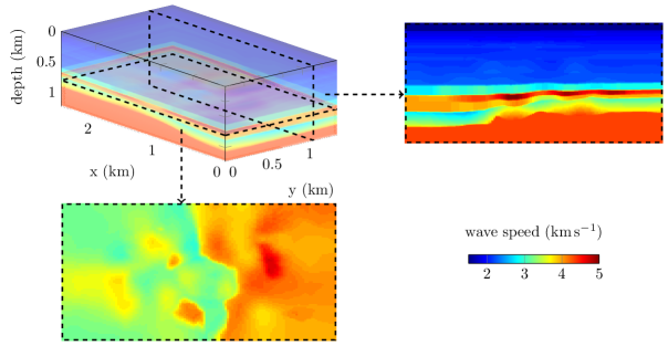
Figure 3: Three-dimensional representation, horizontal section at $800$$\mathrm{m}$ depth and vertical section at $y=1.125$$\mathrm{km}$ of the reference wave speed. It is represented with $1\,527\,168$ nodal values.

The seismic acquisition consists of $\mathrm{missing}\mathrm{revert_as}\mathrm{=}{presentation}\mathrm{]}{}{160}$ sources and $\mathrm{missing}\mathrm{revert_as}\mathrm{=}{presentation}\mathrm{]}{}{1376}$ receivers, that is, dual sensors recording the Cauchy data probed by the sources. The receivers are positioned on a regular $43$ (along the $x$-axis) by $32$ (along the $y$-axis) grid at a fixed depth below the sources lattice. The configuration is illustrated in Figure 4. We consider two situations for the discretized sources map: the sources are first contained in a solid region, in accordance with the above analysis (see Figure 4(b)). Then, they are restricted on a two-dimensional lattice (see Figure 4(c)). The first approach, less common in seismic applications, is yet possible with recent acquisition technique described in Footnote 1, for which the depth of the sources can vary. Following the situation prescribed in Subsection 2.3, we assume that the uppermost part of the model (which is water), in which the Cauchy data are obtained, is known prior to the reconstruction. However, we do not assume the knowledge of the wave speed onto the lateral and bottom boundaries.

We impose a free surface, Dirichlet boundary condition on the top part, $\Gamma_{1}$, of $\partial\Upsilon$ and absorbing boundary conditions on $\Gamma_{2}=\partial\Upsilon\backslash\overline{\Gamma}_{1}$, by taking $k_{0}=kc_{0}^{-1}$ in the third equation of (2.16), following Engquist and Majda [19].

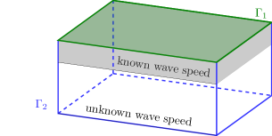
(a) Three-dimensional computational domain.

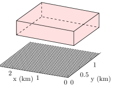
(b) Acquisition with sources contained in a three-dimensional region.

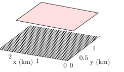
(c) Acquisition with sources contained on a plane.

Figure 4: Illustration of the configuration. (a) We apply a Dirichlet boundary on the upper surface $\Gamma_{1}$ (in green) and absorbing boundary conditions on $\Gamma_{2}=\partial\Upsilon\backslash\overline{\Gamma}_{1}$ (indicated in blue). (b)–(c) The sources that probe the Cauchy data lie in between the receivers and the free surface. Sources are positioned in a three or two-dimensional region (in red). The position of the receivers (black dots) remains fixed. Both receivers and sources lie in the area of known wave speed.

Synthetic dual-sensor data are generated in the time-domain using a Discontinuous Galerkin (DG) finite element method. The original data for a single centered source are presented in Figures 5 and 6 for the pressure and vertical velocity respectively. In the figures, we can observe the difference of scale in the amplitudes between the pressure and the vertical velocity.

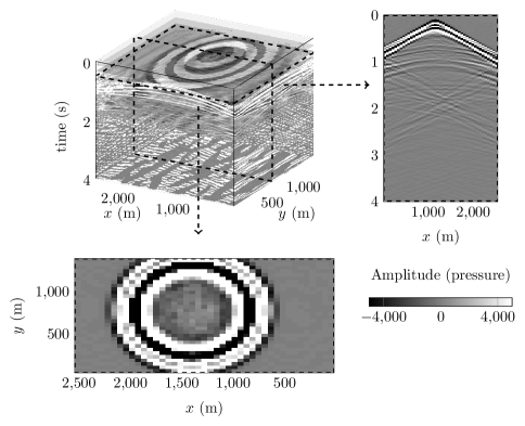
Figure 5: Three-dimensional time-domain pressure trace for a centrally located source. Sections at fixed time $t=0.5$$\mathrm{s}$ and for a fixed line of receivers positioned in $y=695$$\mathrm{m}$ are respectively given at the bottom and right of the $3$D visualization. The $x$ and $y$ axis correspond with the receivers map (i.e., every $60$$\mathrm{m}$ for $x$ and $45$$\mathrm{m}$ for $y$).

Figure 6: Three-dimensional time-domain vertical velocity trace for a centrally located source. Sections at fixed time $t=0.5$$\mathrm{s}$ and for a fixed line of receivers positioned in $y=695$$\mathrm{m}$ are respectively given at the bottom and right of the $3$D visualization. The $x$ and $y$ axis correspond with the receivers map (i.e., every $60$$\mathrm{m}$ for $x$ and $45$$\mathrm{m}$ for $y$).

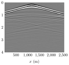
(a) Noiseless synthetic trace section.

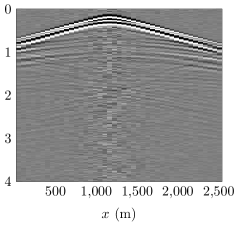
(b) Noisy synthetic trace section using $15$ $\mathrm{dB}$ signal to noise ratio. It is used to generate the frequency data for the reconstruction.

Figure 7: Comparison of noiseless and noisy data for a section of the pressure trace given Figure 5. The noise is independently generated for every receiver and every source in the acquisition.

We subject the (time-domain) data to Gaussian white noise, using a signal-to-noise ratio of $15$$\mathrm{dB}$ (this process is illustrated Figure 7). Note that every receiver for each source has an independent white noise signal added. We apply the Fourier transform to these noisy data and obtain time-harmonic data. The effect of noise affects particularly the low-frequency regime in seismic, and frequencies below $3$ $\mathrm{Hz}$ are usually unusable.

In this experiment we only select $10$$\mathrm{Hz}$ frequency data for the reconstruction algorithm and underlying iterative minimization of the misfit functional (2.27). We simulate time-harmonic data using a Continuous Galerkin finite element method (CG). We use an approach and implementation similar to the one discussed in Shi et al. [35]. The relevant system of equations are solved with the direct structured solver Mumps, [5]. The numerical discretization introduces a tetrahedral representation of the model, which we illustrate in Figure 8.

The choice of CG (instead of DG) is motivated by the memory cost of solving large linear system, which is a specificity of the harmonic case (DG is used for the time-domain discretization). In our experiments, we use order $3$ polynomials to guarantee the accuracy (by taking at least four degrees of freedom per wavelength, according to the common heuristic). Note also that the mesh employed to generate the synthetic (time-domain) data differs from the one used for the inverse (harmonic) problem: the one to generate the data is refined to make sure we consider acutely the variations of the reference wave speed model.

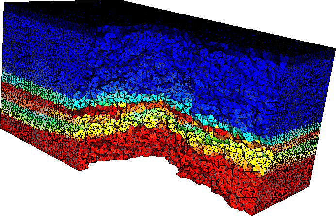
Figure 8: Illustration of the unstructured tetrahedral mesh of the model, using $433\,979$ tetrahedra.

For the reconstruction, the wave speed uses a piecewise linear representation, following (2.5b) and [3]. For the construction of the hierarchy of stable subspaces, the domain partition determining the piecewise linear representation of the wave speed is typically significantly coarser than the tetrahedral mesh. Hence, we define every subdomain, $D_{j}$, as the union of mesh elements, $K_{i}$, according to

(3.1) $$D_{j}=\bigcup_{i=1}^{N_{j}}K_{i},$$

where $N_{j}$ denotes the number of mesh elements in $D_{j}$.

To achieve the decomposition, we apply a structured decision where the maximal size of the subdomains is chosen in every direction to define the subspace. Then, piecewise linear functions are employed onto each generated subdomain to represent the model. We illustrate the effect of piecewise linear partitioning applied on the wave speed model in Figure 9, where the size of the subdomain is at most $400$$\mathrm{m}$ in the $x$ and $y$ directions, and $150$$\mathrm{m}$ in the $z$ direction; this leads to a decomposition with $N=$224$$ subdomains and $896$ coefficients to represent the model. Inherent model error is introduced from those two levels of representation (the mesh and the partitioning). Because we do not know the subsurface geometry a priori, the piecewise linear partition relies on the gradient of the misfit functional instead of the wave speed. Naturally, the more subdomains are taken, the more accurate can the representation be.

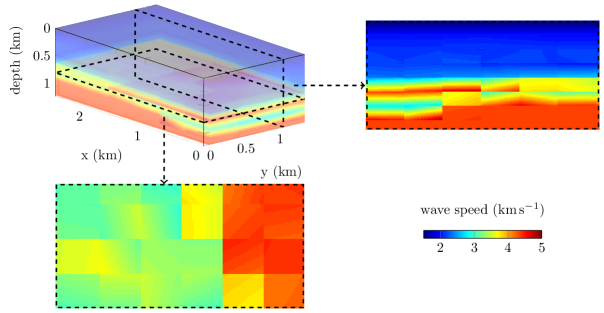
Figure 9: Illustration of three-dimensional partitioning of the wave speed model of Figure 3. The size of subdomains is limited to $400$$\mathrm{m}$ in the $x$ and $y$ directions and $150$$\mathrm{m}$ in the $z$ direction. This leads to a decomposition of $N=$224$$ subdomains where piecewise linear functions are used to represent the wave speed.

We proceed using single-frequency, $10$$\mathrm{Hz}$ data and a fixed domain partition. Exploiting the Lipschitz stability result obtained in Theorem 2 above, the Landweber iteration [18] provides a convergence analysis. The initial model needs to be within the radius of convergence. Algorithm 1 summarizes the steps of the reconstruction procedure.

Preliminary material:

• time-domain observation data at the receivers location,

• user prescribed frequency $k$ and associated partition $N$,

• user prescribed initial model $c_{1}$ and number of iterations $n_{\text{iter}}^{(\min)}$, $n_{\text{iter}}^{(\max)}$,

• user prescribed stagnation parameters $\epsilon_{\mathcal{J}}$ and $n_{\epsilon}$.

Computation of the Fourier transform of the time-domain Cauchy traces at $k$.

Optimization loop for $j\in\{1,\ldots,n_{\text{iter}}^{(\max)}\}$ do

•  

  solve the Helmholtz equation (2.16) at frequency $k$ with wave speed $c_{j}$;

 

compute the misfit functional (2.27) from the simulation and observation data;

 

compute the gradient of the misfit functional, $\nabla\mathcal{J}(c_{j})$ with the adjoint-state method (see Subsection 2.4);

 

compute the search direction, $s_{j}$, here we use the nonlinear conjugate gradient method with Polak–Ribière formula (cf. [28, Section 5.2]);

 

apply segmentation onto the search direction (see illustration on Figure 9);

 

compute the step length $\alpha$ with line search method (backtracking, cf. [28, Chapter 3]);

 

model update $c_{j+1}=c_{j}-\alpha s_{j}$;

       if $j\geq n_{\text{iter}}^{(\min)}$ and $j>n_{\epsilon}$  then

            

• compute the stagnation criterion $\mathfrak{e}=\dfrac{\mathcal{J}(c_{j-n_{\epsilon}})-\mathcal{J}(c_{j})}{\mathcal{J}(c_{j-n_{\epsilon}})};$

• if $(\mathfrak{e}<\epsilon_{\mathcal{J}})$: exit optimization loop.

       end if

      

end for

Algorithm 1 algorithm for the reconstruction of subsurface parameters using piecewise linear model partition and Cauchy data.

Two parameters can decide of the termination of the procedure: if the number of iterations $n_{\text{iter}}^{(\max)}$ is reached, or if the cost function stagnates (criteria $\epsilon_{\mathcal{J}}$ and $n_{\epsilon}$), see Algorithm 1. In the following experiments, we impose

(3.2) $$n_{\text{iter}}^{(\min)}=50,\quad n_{\text{iter}}^{(\max)}=250,$$

$$\quad n_{\epsilon}=10\quad\text{and}\quad\epsilon_{\mathcal{J}}=0.01.$$

Hence, the number of iterations is kept relatively high and the stagnation stops the procedure. More precisely with the given numbers, the algorithm stops if the difference in the misfit functional over the last ten iterations is less than $1$%.

3.1 Single-frequency data

From the Cauchy data at $10$$\mathrm{Hz}$, we carry out a reconstruction of the reference model starting from the smooth model depicted Figure 10. We encode the principal variation and appropriate order of magnitude of the wave speed in the initial model.

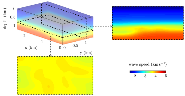
Figure 10: Three-dimensional representation, horizontal section at $800$$\mathrm{m}$ depth and vertical section at $y=1.125$$\mathrm{km}$ of the initial wave speed model.

The model is partitioned in $1089$ subdomains where piecewise linear functions are used to define the wave speed. This leads to a total number of unknowns of $4$$\times$$1089$ = $4356$ (while the reference medium has $1\,527\,168$ nodal values, see Figure 3). The key, here, is the low-dimensional subspace used for regularization. The partition is adapted to the gradient computation via segmentation. We carry out $175$ iterations for the two situations. In Figure 11(a), we show the reconstruction when the sources are positioned in a volume above the receivers (see Figure 4(b)); in Figure 11(b), we show the reconstruction when the sources are restricted on a two-dimensional plane (see Figure 4(c)). To compare the accuracy of the reconstructions, we use the relative $L^{2}$ norm of the difference between the reference model and the reconstruction:

(3.3) $$\text{relative $L^{2}$ error}=\mathcal{E}_{\text{rel}}=\dfrac{\|c_{\dagger}-c_{\text{r}}\|}{\|c_{\dagger}\|},$$

where $c_{\dagger}$ is the reference model of Figure 3 and $c_{\text{r}}$ the final reconstruction.

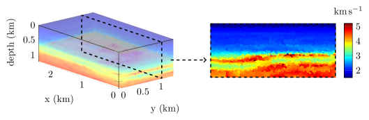
(a) Reconstruction where the sources in the acquisition are positioned in a three-dimensional area (see Figure 4(b)); the relative $L^{2}$ difference with the reference model Figure 3 is $\mathcal{E}_{\text{rel}}=0.083$.

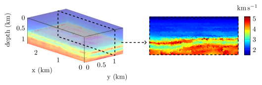
(b) Reconstruction where the sources in the acquisition are limited on a plane (see Figure 4(c)); the relative $L^{2}$ difference with the reference model Figure 3 is $\mathcal{E}_{\text{rel}}=0.088$.

Figure 11: Three-dimensional representation and vertical section at $y=1.125$$\mathrm{km}$ of the reconstruction from $10$$\mathrm{Hz}$ Cauchy data after $175$ iterations. The partition consists of $N=1089$ subdomains, leading to a total number of unknowns of $4\times 1089=4356$. The initial model is shown in Figure 10.

The two acquisitions provide accurate recoveries of the subsurface, with some improvement when the sources are positioned in a volume: the width of the increased wave speed layer and the deepest values of the wave speed are better retrieved with this type of acquisition. However, the reconstruction from sources limited on a plane is very close. In the subspace, we have drastically reduced the number of unknowns in the representation as compared with the original representation, namely to $0.3\%$. Nonetheless, the reconstruction captures the main features of the model, including the alternation of high and low values in the vertical direction and the resolution remains reasonable.

Remark 2 (Improved visualization with Gaussian filtering).

The visualization of the reconstruction may suffer from the tetrahedral mesh employed for the numerical discretization. It is simple to improve the visualization by applying a smoothing filter onto the image. This can be done, for example, with the imgaussfilt function of MATLAB, which applies a Gaussian smoothing filter. In Figure 12, we show the resulting image when applied onto the reconstruction of Figure 11(b). It allows a better identification of the recovered structures. Note that this procedure is done a-posteriori, independently of the reconstruction algorithm, and is effortless.

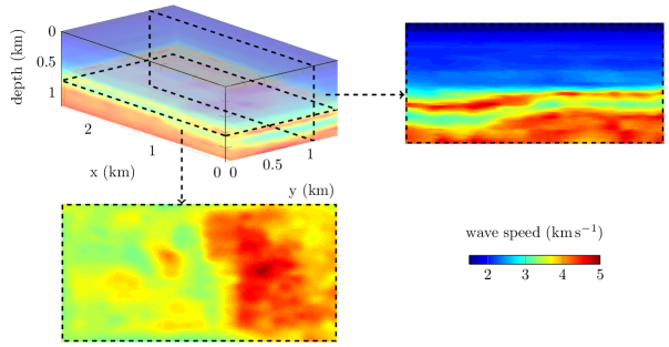
Figure 12: Gaussian filtering of the reconstruction obtained from $10$$\mathrm{Hz}$ Cauchy data (Figure 11(b)), three-dimensional representation, horizontal section at $800$$\mathrm{m}$ depth and vertical section at $y=1.125$$\mathrm{km}$. The relative $L^{2}$ difference with the reference model Figure 3 is $\mathcal{E}_{\text{rel}}=0.079$.

In the following experiments, we only consider the case where sources are restricted on a plane, following the acquisition illustrated Figure 4(c), for simplicity.

3.2 Single-frequency data, depth varying initial model

We repeat the experiment carried out in the previous subsection (with the two-dimensional sources lattice), but with a simplified initial model, see Figure 13. That is, here, the initial model only contains an indication of the average variation of wave speed in depth. The idea behind this experiment is to test the radius of convergence on the one hand, and the closeness of the true model and the best projection onto a low-dimensional stable subspace on the other hand.

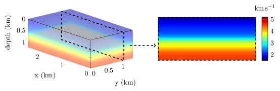
Figure 13: Three-dimensional representation and vertical section at $y=1.125$$\mathrm{km}$ of the initial model, which varies in depth only.

In Figures 14 and 15, we present the result after $175$ iterations using $10$$\mathrm{Hz}$ Cauchy data. As in the first experiment, we have $1089$ subdomains in the partition and piecewise linear representations. Despite the lack of initial information we still retrieve the main features and appropriate contrasts in the wave speed. However, we lost accuracy as compared with the previous example (especially on the side), but the deep layer of low wave speed is well identified nonetheless.

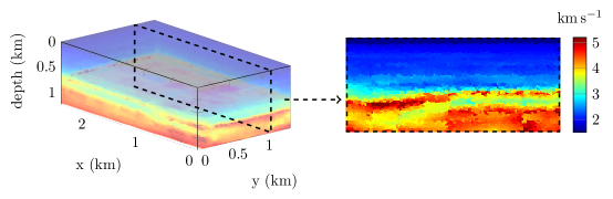
Figure 14: Three-dimensional representation and vertical section at $y=1.125$$\mathrm{km}$ of the reconstruction from $10$$\mathrm{Hz}$ Cauchy data after $175$ iterations. The partition consists of $N=1089$ subdomains, leading to a total number of unknowns of $4\times 1089=4356$. The initial model varies in depth only and is shown in Figure 13. The relative $L^{2}$ difference with the reference model Figure 3 is $\mathcal{E}_{\text{rel}}=0.119$.

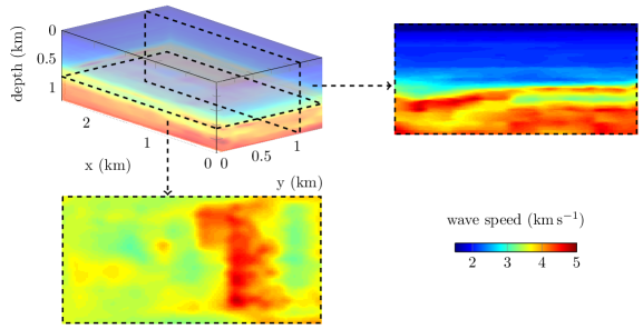
Figure 15: Gaussian filtering (see Remark 2) of the reconstruction (Figure 14) obtained from $10$$\mathrm{Hz}$ Cauchy data starting with the initial model that varies in depth only (Figure 13). Three-dimensional representation, horizontal section at $800$$\mathrm{m}$ depth and vertical section at $y=1.125$$\mathrm{km}$. The relative $L^{2}$ difference with the reference model Figure 3 is $\mathcal{E}_{\text{rel}}=0.108$.

In Figure 16, we show the evolution of the misfit functional with iterations on a logarithmic scale, where we compare with the previous experiment that used a smooth initial model (see Figure 10 and Figure 11(b) for the reconstruction). As expected, the first iteration using the smooth initial model provides a reduction in the misfit functional compared to the one-dimensional starting model. The decrease of the misfit functional is relatively fast for the initial iterations, especially when starting with the smooth model, and we observe a slow evolution after about $100$ iterations in both configurations. Eventually, we observe the stagnation which stops the procedure. As indicated with the $L^{2}$ norm of the difference between the reference model (see Figures 11(b) and 14), starting with the smooth model provides a better approximation.

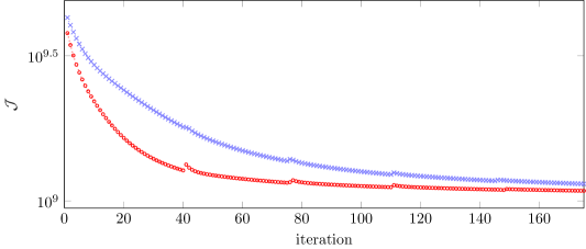
Figure 16: Evolution of the misfit functional with iterations, the blue crosses correspond with the case where the initial model is one-dimensional (see Figure 13 for the initial model and Figure 14 for the associated reconstruction); the red circles correspond with the case where the initial model is smooth (see Figure 10 for the initial model and Figure 11(b) for the associated reconstruction).

Figures 17 and 18 compare the observed, initial and reconstruction data, using the full receivers map associated with a centrally located source. We see that the data from the recovered wave speed provide a pattern that is similar to the Fourier transform of the time-domain observations.

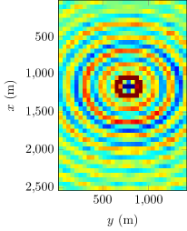
(a) Fourier transform of the time-domain observation.

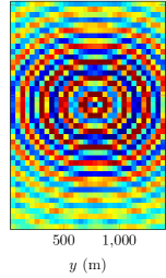
(b) Simulated data using the initial model of Figure 13.

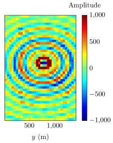
(c) Simulated data from the reconstructed model Figure 14.

Figure 17: Comparison of the $10$$\mathrm{Hz}$ frequency pressure data captured at the receivers location for a centrally located source.

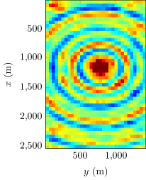
(a) Fourier transform of the time-domain observation.

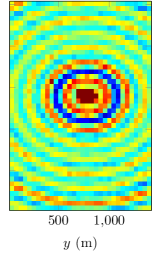
(b) Simulated data using the initial model of Figure 13.

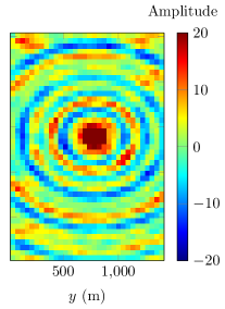
(c) Simulated data from the reconstructed model Figure 14.

Figure 18: Comparison of the $10$$\mathrm{Hz}$ frequency vertical velocity data captured at the receivers location for a centrally located source.

4 Perspectives on independent locations of sources in the discretized settings

The misfit functional (2.27) defined for the Cauchy data has an interesting feature, because of the intuitive differentiation between acquisition sets for the observations and simulations. It is materialized by the double integral over $K_{1}\times K_{1}$. The perspective is here to separate in, say, $K_{2}\times K_{1}$.

In the usual context of minimization involving the direct difference between observations and simulations, such as the standard least squares, the setup for simulation is imposed by the field acquisition (source position and wavelet). Consequently, absence of knowledge leads to the failure of the algorithm. Here, providing this new misfit functional, we expect our iterative minimization algorithm to be free of those considerations, introducing extreme flexibility for the setup, where only the position of the receivers is required.

To illustrate the potential of the method, we design an experiment where the simulation sources differ from the observational ones. We consider a subsurface wave speed model where salt domes (objects having a large speed contrast) are present. The model is illustrated in Figure 19 and is of size $2.46\times 1.56\times 1.2$$\mathrm{km}$. It consists in a smooth background with contrasting objects having a wave speed of $4500$$\mathrm{m}\text{\,}{\mathrm{s}}^{-1}$. We assume that the density remains constant with $\rho=1000$$\mathrm{kg}\text{\,}{\mathrm{m}}^{-3}$. This medium is very different in nature from the previous one, and salt domes are traditionally challenging in seismic exploration (especially where their presence is initially unknown).

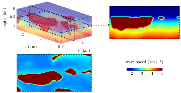
Figure 19: Three-dimensional representation, horizontal section at $550$$\mathrm{m}$ depth and vertical section at $y=670$$\mathrm{m}$ of the reference wave speed encompassing salt domes. The wave speed in the domes is a constant of $4500$$\mathrm{m}\text{\,}{\mathrm{s}}^{-1}$.

Time-domain Cauchy data are obtained from this configuration with $1000$ fixed receivers for each of the $96$ sources. Here the sources are positioned on a plane, according to Figure 4(c). The devices are located just underneath the surface, at a depth of $10$$\mathrm{m}$ for the source and $100$$\mathrm{m}$ for the receivers. We incorporate noise in the time-domain data, with a signal-to-noise ratio of $15$$\mathrm{dB}$, before we proceed to the Fourier transform to get the frequency-domain data. For the reconstruction we start with an initial model which only varies with depth, see Figure 20. We do not assume any contrasting objects in our initial guess, nor do we know the value for the background. For the reconstruction we only assume the knowledge of the uppermost water layer (up to $150$$\mathrm{m}$ depth).

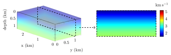
Figure 20: Three-dimensional representation and vertical section at $y=670$$\mathrm{m}$ of the initial model, which varies in depth only.

To differentiate the simulation set of sources from the observation, we reduce their number, change their position and modify the source wavelet, see Table 1. We perform $100$ iterations of the reconstruction Algorithm 1, with single frequency data at $4$$\mathrm{Hz}$. The model representation is fixed with $N=1280$ sub-domains where piecewise linear functions are employ, for a total of $5120$ coefficients.

	Setup for measurements	Setup for simulations
Number of sources	96	60
Depth of the sources	10$\mathrm{m}$	20$\mathrm{m}$

Table 1: Comparison of acquisition setups employed for the observations and simulations. The source wavelet also differs. For the reconstruction, single frequency data at $4$$\mathrm{Hz}$ and a fixed model partition of $N=1280$ are used.

The reconstruction after $100$ iterations is shown Figures 21 and 22. Despite our initial guess having no information on the objects, the procedure is able to recover the main dome with the accurate value, and the shape of smaller domes (see the horizontal section in Figure 22). The near boundary information seems missing, as well as the deepest model variation, due to limited illumination. However, as we started with a one dimensional guess and used single frequency data, the reconstruction is very satisfactory. Once again, the restricted number of unknowns does not prevent a good resolution.

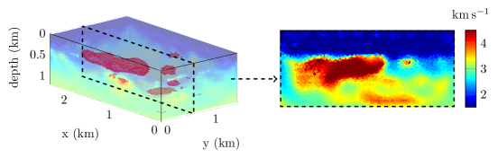
Figure 21: Three-dimensional representation and vertical section at $y=670$$\mathrm{m}$ of the reconstruction using $4$$\mathrm{Hz}$ Cauchy data after $100$ iterations and where the simulation setup differs from the original measurement acquisition, see Table 1. The relative $L^{2}$ difference with the reference model Figure 19 is $\mathcal{E}_{\text{rel}}=0.174$.

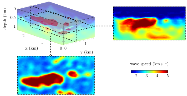
Figure 22: Gaussian filtering (see Remark 2) of the reconstruction (Figure 21) obtained using $100$ iterations with $4$$\mathrm{Hz}$ Cauchy data and where the setup for simulation differs from the original measurement acquisition. Three-dimensional representation, horizontal section at $550$$\mathrm{m}$ depth and vertical section at $y=670$$\mathrm{m}$. The relative $L^{2}$ difference with the reference model Figure 19 is $\mathcal{E}_{\text{rel}}=0.172$.

We have changed the number of sources in the simulation compared to the observation, reducing the numerical cost accordingly, yet we make full use of the observed data from the benefit of our misfit functional defined for Cauchy data. Furthermore we do not need to know the position of the sources employed for observation, nor the source wavelet. The perspective of differentiating the observations and simulations acquisition sets is a promising application, and appears consistent with the results of this preliminary experiment. It would allow less prior on the observational environment, increasing the robustness of the procedure, without impacting the resolution of the reconstruction.

5 Acknowledgment

The research of G. Alessandrini and E. Sincich for the preparation of this paper has been supported by FRA 2016 “Problemi inversi, dalla stabilità alla ricostruzione”, funded by Università degli Studi di Trieste. Maarten V. de Hoop acknowledges the Simons Foundation under the MATH+X program for financial support. He was also partially supported by NSF under grant DMS–1559587. R. Gaburro wishes to acknowledge the support of MACSI, the Mathematics Applications Consortium for Science and Industry (www.macsi.ul.ie), funded by the Science Foundation Ireland Investigator Award 12/IA/1683. E. Sincich has also been supported by Gruppo Nazionale per l’Analisi Matematica, la Probabilità e le loro Applicazioni (GNAMPA) by the grant “Analisi di problemi inversi: stabilità e ricostruzione”. The research of F. Faucher is supported by the Inria–TOTAL strategic action DIP.

References

- [1] R. A. Adams and J. J. F. Fournier, Sobolev Spaces, Elsevier Science, 2003.
- [2] V. Akcelik, G. Biros and O. Ghattas, Parallel Multiscale Gauss-Newton-Krylov Methods for Inverse Wave Propagation, Supercomputing, ACM/IEEE 2002 Conference (2002), 41pp.
- [3] G. Alessandrini, M.V. de Hoop, R. Gaburro and E. Sincich, Lipschitz stability for a piecewise linear Schrödinger potential from local Cauchy data, Asymptotic Analysis, 108 (3) (2018), 115–149.
- [4] G. Alessandrini and S. Vessella, Lipschitz stability for the inverse conductivity problem, Advances in Applied Mathematics, 35 (2) (2005), 207–241.
- [5] P. R. Amestoy, A. Guermouche, J.-Y. L’Excellent and S. Pralet, Hybrid scheduling for the parallel solution of linear systems, Parallel computing, 32 (2) (2006), 136–156.
- [6] J. B. Bednar, C. Shin and S. Pyun, Comparison of waveform inversion, part 2: phase approach, Geophysical Prospecting 55 (4) (2007), 465-475.
- [7] E. Beretta, M. De Hoop and L. Qiu, Lipschitz stability of an inverse boundary value problem for a Schrödinger type equation, SIAM J. Math. Anal. 45 (2) (2013), 679-699.
- [8] E. Bozdağ, J. Trampert and J. Tromp, Misfit functions for full waveform inversion based on instantaneous phase and envelope measurements Geophysical Journal International 85 (2) (2011), 845–870.
- [9] R. Brossier, S. Operto and J. Virieux, Robust elastic frequency-domain full-waveform inversion using the norm Geophysical Research Letters 36 (20) (2009).
- [10] R. Brossier, S. Operto and J. Virieux, Which data residual norm for robust elastic frequency-domain full waveform inversion? Geophysics 75 (3) (2010), R37–R46.
- [11] C. Bunks, F. M. Saleck, S. Zaleski and G. Chavent, Multiscale seismic waveform inversion, Geophysics 60 (5) (1995), 1457-1473.
- [12] F. Cakoni and D. L. Colton, A qualitative approach to inverse scattering theory, Springer (2014).
- [13] D. Carlson, W. Söllner, H. Tabti, E. Brox and M. Widmaier, Increased resolution of seismic data from a dual-sensor streamer cable, SEG Technical Program Expanded Abstracts 2007, 994–998, Society of Exploration Geophysicists (2007).
- [14] C. I. Cârstea, N. Honda and G. Nakamura, Uniqueness in the inverse boundary value problem for piecewise homogeneous anisotropic elasticity, arXiv preprint arXiv:1611.03930v2 (2016).
- [15] G. Chavent, Identification of functional parameters in partial differential equations, Identification of Parameters in Distributed Systems (1974).
- [16] G. Chavent, Nonlinear least squares for inverse problems: theoretical foundations and step-by-step guide for applications. Springer Science & Business Media (2010).
- [17] D. Colton and H. Haddar, An application of the reciprocity gap functional to inverse scattering theory, Inverse Problems 21 (1) (2005), 383–398.
- [18] M. De Hoop, L. Qiu and O. Scherzer, Local analysis of inverse problems: Hölder stability and iterative reconstruction, Inverse Problems 28 (4) (2012): 045001.
- [19] B. Engquist and A. Majda, Absorbing boundary conditions for numerical simulation of waves, Proceedings of the National Academy of Sciences 74 (5) (1977), 1765–1766
- [20] M. Ikehata, Reconstruction of the shape of the inclusion by boundary measurements, Communications in Partial Differential Equations 23 (1998), 1459–1474
- [21] B. L. N. Kennett, M. S. Sambridge and P. R. Williamson, Subspace methods for large inverse problems with multiple parameter classes, Geophysical Journal International 94 (1988), 237–247.
- [22] M. Kern, Numerical Methods for Inverse Problems. John Wiley & Sons (2016).
- [23] P. Lailly, The seismic inverse problem as a sequence of before stack migrations, Conference on Inverse Scattering: Theory and Application, Society for Industrial and Applied Mathematics, 206-220, J. B. Bednar, (1983).
- [24] J. L. Lions and S. K. Mitter, Optimal control of systems governed by partial differential equations, Springer Berlin (1971).
- [25] Y. Lin, A. Abubakar and T. M. Habashy, Seismic full-waveform inversion using truncated wavelet representations, in SEG Technical Program Expanded Abstracts 2012, chapter 486 (2012), 1-6.
- [26] I. Loris, H. Douma, G. Nolet, I. Daubechies and C. Regone, Nonlinear regularization techniques for seismic tomography, Journal of Computational Physics 229 (2010), 890-905.
- [27] I. Loris, G. Nolet, I. Daubechies and F.A. Dahlen, Tomographic inversion using L1-norm regularization of wavelet coefficients, Geophysical Journal International 170 (2007), 359-370.
- [28] J. Nocedal and S. Wright, Numerical optimization, Second Edition, Springer series in operations research (2006).
- [29] G. S. Pan, R. A. Phinney and R. I. Odom, Full-waveform inversion of plane-wave seismograms in stratified acoustic media; theory and feasibility, Geophysics 53 (1) (1988), 21-31.
- [30] R.-E. Plessix, A review of the adjoint-state method for computing the gradient of a functional with geophysical applications, Geophysical Journal International 167 (2) (2006), 495–503.
- [31] R. Potthast, A survey on sampling and probe methods for inverse problems, Inverse Problems 22 (2) (2006), R1–R47.
- [32] R. G. Pratt, Z.-M. Song, P. Williamson and M. Warner, Two-dimensional velocity models from wide-angle seismic data by wavefield inversion, Geophysical Journal International 124 (1996), 323-340.
- [33] R. G. Pratt and M. H. Worthington, Inverse theory applied to multi-source cross-hole tomography. Part 1: Acoustic wave-equation method, Geophysical Prospecting 38 (1990), 287-310.
- [34] G. Rønholt, J. E. Lie, O. Korsmo, B. Danielsen, S. Brandsberg-Dah, S. Brown, N. Chemingui, A Valenciano Mavilio, D. Whitmore and R. D. Martinez, Broadband velocity model building and imaging using reflections, refractions and multiples from dual-sensor streamer data, 14th International Congress of the Brazilian Geophysical Society & EXPOGEF, Rio de Janeiro, Brazil, 3-6 August 2015, 1006-1009, Brazilian Geophysical Society (2015).
- [35] J. Shi, M.V. de Hoop, E. Beretta, E. Francini and S. Vessella, Multi-parameter iterative reconstruction with the Neumann-to-Dirichlet map as the data, preprint (2017).
- [36] S. Pyun, C. Shin, and J. B. Bednar, Comparison of waveform inversion, part 3: amplitude approach, Geophysical Prospecting, 55 (4) (2007), 477-485.
- [37] C. Shin, S. Pyun, and J. B. Bednar, Comparison of waveform inversion, part 1: conventional wavefield vs logarithmic wavefield, Geophysical Prospecting, 55 (4) (2007), 449-464.
- [38] A. Tarantola, Inversion of seismic reflection data in the acoustic approximation, Geophysics 49 (1984), 1259-1266.
- [39] A. Tarantola, Inversion of travel times and seismic waveforms, Seismic tomography, 135 - 157, Springer, (1987).
- [40] R. Tenghamn, S. Vaage and C. Borresen, A dual-sensor towed marine streamer: Its viable implementation and initial results, SEG Technical Program Expanded Abstracts 2007, 989–993, Society of Exploration Geophysicists (2007).
- [41] N. D. Whitmore, A. A. Valenciano, W. Sollner and S. Lu, Imaging of primaries and multiples using a dual-sensor towed streamer, SEG Technical Program Expanded Abstracts 2010, 3187–3192, Society of Exploration Geophysicists (2010).
- [42] R.-S. Wu, J. Luo and B. Wu, Seismic envelope inversion and modulation signal model, Geophysics 79 (3) (2014), WA13–WA24.
- [43] Y. O. Yuan and F. J. Simons, Multiscale adjoint waveform-difference tomography using wavelets, Geophysics 79 (3), Society of Exploration Geophysicists (2014), WA79–WA95.
- [44] Y. O. Yuan, F. J. Simons and E. Bozdağ, Multiscale adjoint waveform tomography for surface and body waves, Geophysics 80 (5), Society of Exploration Geophysicists (2015), R281–R302.