An adaptive fast Gauss transform in two dimensions

Jun Wang Courant Institute of Mathematical Sciences, New York University, New York, New York 10012. (Present address: Flatiron Institute, Simons Foundation, New York, New York 10010. Email: junwang@flatironinstitute.org.)    Leslie Greengard Courant Institute of Mathematical Sciences, New York University, New York, New York 10012 and Flatiron Institute, Simons Foundation, New York, New York 10010. This work was supported in part by the Applied Mathematical Sciences Program of the U.S. Department of Energy under Contract DEFGO288ER25053 and by the RiskEcon Lab for Decision Metrics, Courant Institute. Email: greengard@cims.nyu.edu.
Abstract

A variety of problems in computational physics and engineering require the convolution of the heat kernel (a Gaussian) with either discrete sources, densities supported on boundaries, or continuous volume distributions. We present a unified fast Gauss transform for this purpose in two dimensions, making use of an adaptive quad-tree discretization on a unit square which is assumed to contain all sources. Our implementation permits either free-space or periodic boundary conditions to be imposed, and is efficient for any choice of variance in the Gaussian.

keywords:
fast Gauss transform, heat equation, adaptive mesh refinement
AMS:
31A10 35K10 65R10 65Y20

1 Introduction

A variety of problems in applied physics and engineering involve the solution of the heat equation

ut(𝐱,t)=Δu(𝐱,t)+F(𝐱,t)u(𝐱,0)=f(𝐱)subscript𝑢𝑡𝐱𝑡Δ𝑢𝐱𝑡𝐹𝐱𝑡𝑢𝐱0𝑓𝐱\begin{split}u_{t}({\bf x},t)&=\Delta u({\bf x},t)+F({\bf x},t)\\ u({\bf x},0)&=f({\bf x})\end{split} (1)

for t>0𝑡0t>0, in a interior or exterior domain ΩΩ\Omega, subject to suitable conditions on its boundary Γ=ΩΓΩ\Gamma=\partial\Omega. For simplicity, we will assume that these take the form of either Neumann conditions:

un(𝐱,t)=g(𝐱,t)for𝐱Γ,formulae-sequence𝑢𝑛𝐱𝑡𝑔𝐱𝑡for𝐱Γ\frac{\partial u}{\partial n}({\bf x},t)=g({\bf x},t)\ \ {\rm for}\quad{\bf x}\in\Gamma, (2)

Dirichlet conditions:

u(𝐱,t)=h(𝐱,t)for𝐱Γ,formulae-sequence𝑢𝐱𝑡𝐱𝑡for𝐱Γu({\bf x},t)=h({\bf x},t)\ \ {\rm for}\quad{\bf x}\in\Gamma, (3)

or periodic boundary conditions with ΩΩ\Omega the unit square.

In the absence of physical boundaries, the equations (1) are well-posed in free space (under mild conditions on the behavior of u𝑢u, f𝑓f and F𝐹F at infinity) without auxiliary conditions. Moreover, assuming F(𝐱,t)𝐹𝐱𝑡F({\bf x},t) and f(𝐱)𝑓𝐱f({\bf x}) are compactly supported in the region ΩΩ\Omega, the solution to (1) can be expressed at the next time step, t=Δt𝑡Δ𝑡t=\Delta t in closed form as

u(𝐱,Δt)=J[f](𝐱,Δt)+V[F](𝐱,Δt)𝑢𝐱Δ𝑡𝐽delimited-[]𝑓𝐱Δ𝑡𝑉delimited-[]𝐹𝐱Δ𝑡u({\bf x},\Delta t)=J[f]({\bf x},\Delta t)+V[F]({\bf x},\Delta t) (4)

with

J[f](𝐱,Δt)𝐽delimited-[]𝑓𝐱Δ𝑡\displaystyle J[f]({\bf x},\Delta t) =ΩG(𝐱𝐲,Δt)f(𝐲)𝑑𝐲absentsubscriptΩ𝐺𝐱𝐲Δ𝑡𝑓𝐲differential-d𝐲\displaystyle=\int_{\Omega}G({\bf x}-{\bf y},\Delta t)f({\bf y})\,d{\bf y} (5)
V[F](𝐱,Δt)𝑉delimited-[]𝐹𝐱Δ𝑡\displaystyle V[F]({\bf x},\Delta t) =0ΔtΩG(𝐱𝐲,Δtτ)F(𝐲,τ)𝑑𝐲𝑑τ.absentsuperscriptsubscript0Δ𝑡subscriptΩ𝐺𝐱𝐲Δ𝑡𝜏𝐹𝐲𝜏differential-d𝐲differential-d𝜏\displaystyle=\int_{0}^{\Delta t}\int_{\Omega}G({\bf x}-{\bf y},\Delta t-\tau)F({\bf y},\tau)\,d{\bf y}d\tau\,. (6)

Here,

G(𝐱,t)=e𝐱2/4t(4πt)d/2𝐺𝐱𝑡superscript𝑒superscriptnorm𝐱24𝑡superscript4𝜋𝑡𝑑2G({\bf x},t)=\frac{e^{-\|{\bf x}\|^{2}/4t}}{(4\pi t)^{d/2}}

is the fundamental solution of the heat equation in d𝑑d dimensions. The functions J[f]𝐽delimited-[]𝑓J[f] and V[F]𝑉delimited-[]𝐹V[F] are referred to as initial (heat) potentials and domain (heat) potentials, respectively. In the remainder of this paper, we assume d=2𝑑2d=2.

For the Neumann problem (1), (2), the classical representation [16, 23] takes the form

u(𝐱,Δt)=J[f](𝐱,Δt)+V[F](𝐱,Δt)+S[σ](𝐱,Δt)𝑢𝐱Δ𝑡𝐽delimited-[]𝑓𝐱Δ𝑡𝑉delimited-[]𝐹𝐱Δ𝑡𝑆delimited-[]𝜎𝐱Δ𝑡u({\bf x},\Delta t)=J[f]({\bf x},\Delta t)+V[F]({\bf x},\Delta t)+S[\sigma]({\bf x},\Delta t) (7)

where

S[σ](𝐱,Δt)𝑆delimited-[]𝜎𝐱Δ𝑡\displaystyle S[\sigma]({\bf x},\Delta t) =0ΔtΓG(𝐱𝐲,Δtτ)σ(𝐲,τ)𝑑s𝐲𝑑τabsentsuperscriptsubscript0Δ𝑡subscriptΓ𝐺𝐱𝐲Δ𝑡𝜏𝜎𝐲𝜏differential-dsubscript𝑠𝐲differential-d𝜏\displaystyle=\int_{0}^{\Delta t}\int_{\Gamma}G({\bf x}-{\bf y},\Delta t-\tau)\sigma({\bf y},\tau)\,\,ds_{{\bf y}}d\tau (8)

is a single layer (heat) potential. For the Dirichlet problem (1), (3), the classical representation takes the form

u(𝐱,Δt)=J[f](𝐱,Δt)+V[F](𝐱,Δt)+D[μ](𝐱,Δt)𝑢𝐱Δ𝑡𝐽delimited-[]𝑓𝐱Δ𝑡𝑉delimited-[]𝐹𝐱Δ𝑡𝐷delimited-[]𝜇𝐱Δ𝑡u({\bf x},\Delta t)=J[f]({\bf x},\Delta t)+V[F]({\bf x},\Delta t)+D[\mu]({\bf x},\Delta t) (9)

where

D[μ](𝐱,Δt)𝐷delimited-[]𝜇𝐱Δ𝑡\displaystyle D[\mu]({\bf x},\Delta t) =0ΔtΓGn𝐲(𝐱𝐲,Δtτ)μ(𝐲,τ)𝑑s𝐲𝑑τabsentsuperscriptsubscript0Δ𝑡subscriptΓ𝐺subscript𝑛𝐲𝐱𝐲Δ𝑡𝜏𝜇𝐲𝜏differential-dsubscript𝑠𝐲differential-d𝜏\displaystyle=\int_{0}^{\Delta t}\int_{\Gamma}\frac{\partial G}{\partial n_{{\bf y}}}({\bf x}-{\bf y},\Delta t-\tau)\mu({\bf y},\tau)\,\,ds_{{\bf y}}d\tau (10)

is a double layer (heat) potential. Here, n𝐲subscript𝑛𝐲\frac{\partial}{\partial n_{{\bf y}}} denotes the derivative in the outward normal direction at the boundary point 𝐲𝐲{\bf y}. The only unknowns in the representations (7), (9) are the scalar densities σ𝜎\sigma and μ𝜇\mu supported on ΓΓ\Gamma. These are obtained by solving integral equations to enforce the desired boundary conditions [16, 23]. Once σ𝜎\sigma or μ𝜇\mu is known, (7), (9) can be used to evaluate the solution at time t=Δt𝑡Δ𝑡t=\Delta t. This yields a one-step marching method for the heat equation that is unconditionally stable (see, for example, [1, 5, 7, 8, 12, 17, 21, 29, 30]).

For our present purposes, we assume that σ𝜎\sigma and μ𝜇\mu are given. We assume also that a suitable M𝑀M-stage quadrature has been applied to V[F](𝐱,Δt)𝑉delimited-[]𝐹𝐱Δ𝑡V[F]({\bf x},\Delta t), S[σ](𝐱,Δt)𝑆delimited-[]𝜎𝐱Δ𝑡S[\sigma]({\bf x},\Delta t) and D[σ](𝐱,Δt)𝐷delimited-[]𝜎𝐱Δ𝑡D[\sigma]({\bf x},\Delta t) with respect to the time variable, yielding:

V[F](𝐱,Δt)𝑉delimited-[]𝐹𝐱Δ𝑡\displaystyle V[F]({\bf x},\Delta t) j=1MwV,jΩG(𝐱𝐲,Δtτj)F(𝐲,τj)𝑑𝐲,absentsuperscriptsubscript𝑗1𝑀subscript𝑤𝑉𝑗subscriptΩ𝐺𝐱𝐲Δ𝑡subscript𝜏𝑗𝐹𝐲subscript𝜏𝑗differential-d𝐲\displaystyle\approx\sum_{j=1}^{M}w_{V,j}\int_{\Omega}G({\bf x}-{\bf y},\Delta t-\tau_{j})F({\bf y},\tau_{j})\,d{\bf y}\,,
S[σ](𝐱,Δt)𝑆delimited-[]𝜎𝐱Δ𝑡\displaystyle S[\sigma]({\bf x},\Delta t) j=1MwS,jΓG(𝐱𝐲,Δtτj)σ(𝐲,τj)𝑑s𝐲,absentsuperscriptsubscript𝑗1𝑀subscript𝑤𝑆𝑗subscriptΓ𝐺𝐱𝐲Δ𝑡subscript𝜏𝑗𝜎𝐲subscript𝜏𝑗differential-dsubscript𝑠𝐲\displaystyle\approx\sum_{j=1}^{M}w_{S,j}\int_{\Gamma}G({\bf x}-{\bf y},\Delta t-\tau_{j})\sigma({\bf y},\tau_{j})\,ds_{{\bf y}}\,, (11)
D[μ](𝐱,Δt)𝐷delimited-[]𝜇𝐱Δ𝑡\displaystyle D[\mu]({\bf x},\Delta t) j=1MwD,jΓGn𝐲(𝐱𝐲,Δtτj)μ(𝐲,τj)𝑑s𝐲,absentsuperscriptsubscript𝑗1𝑀subscript𝑤𝐷𝑗subscriptΓ𝐺subscript𝑛𝐲𝐱𝐲Δ𝑡subscript𝜏𝑗𝜇𝐲subscript𝜏𝑗differential-dsubscript𝑠𝐲\displaystyle\approx\sum_{j=1}^{M}w_{D,j}\int_{\Gamma}\frac{\partial G}{\partial n_{{\bf y}}}({\bf x}-{\bf y},\Delta t-\tau_{j})\mu({\bf y},\tau_{j})\,ds_{{\bf y}}\,,

where wV,jsubscript𝑤𝑉𝑗w_{V,j}, wS,jsubscript𝑤𝑆𝑗w_{S,j}, wD,jsubscript𝑤𝐷𝑗w_{D,j} are known quadrature weights.

Thus, the computational burden of time-marching (that is, evaluating the various heat potentials) is dominated by the volume integrals

𝒱[f](𝐱)=Ωe|𝐱𝐲|2δf~(𝐲)𝑑𝐲𝒱delimited-[]𝑓𝐱subscriptΩsuperscript𝑒superscript𝐱𝐲2𝛿~𝑓𝐲differential-d𝐲{\cal V}[f]({\bf x})=\int_{\Omega}e^{-\frac{|{\bf x}-{\bf y}|^{2}}{\delta}}\tilde{f}({\bf y})\,d{\bf y} (12)

and the boundary integrals

𝒮[σ](𝐱)=Γe|𝐱𝐲(s)|2δσ~(𝐲(s))𝑑s𝐲,𝒟[μ](𝐱)=Γn𝐲(s)e|𝐱𝐲(s)|2δμ~(𝐲(s))𝑑s𝐲,formulae-sequence𝒮delimited-[]𝜎𝐱subscriptΓsuperscript𝑒superscript𝐱𝐲𝑠2𝛿~𝜎𝐲𝑠differential-dsubscript𝑠𝐲𝒟delimited-[]𝜇𝐱subscriptΓsubscript𝑛𝐲𝑠superscript𝑒superscript𝐱𝐲𝑠2𝛿~𝜇𝐲𝑠differential-dsubscript𝑠𝐲\begin{split}{\cal S}[\sigma]({\bf x})&=\int_{\Gamma}e^{-\frac{|{\bf x}-{\bf y}(s)|^{2}}{\delta}}\tilde{\sigma}({\bf y}(s))\,ds_{{\bf y}}\,,\\ {\cal D}[\mu]({\bf x})&=\int_{\Gamma}\frac{\partial}{\partial n_{{\bf y}(s)}}e^{-\frac{|{\bf x}-{\bf y}(s)|^{2}}{\delta}}\tilde{\mu}({\bf y}(s))\,ds_{{\bf y}}\,,\end{split} (13)

for various values of δ𝛿\delta and given functions f~,σ~,μ~~𝑓~𝜎~𝜇\tilde{f},\tilde{\sigma},\tilde{\mu}. Evaluating these integrals accurately and efficiently is the focus of the present paper.

Definition 1.

The integrals (12) and (13) will be referred to as volume and boundary Gauss transforms, respectively.

Definition 2.

By the discrete Gauss transform (DGT), we mean the evaluation of the Gaussian “potential” at M𝑀M points {𝐱i}subscript𝐱𝑖\{{\bf x}_{i}\} due to N𝑁N sources located at {𝐲j}subscript𝐲𝑗\{{\bf y}_{j}\} of strength {qj}subscript𝑞𝑗\{q_{j}\}:

F(𝐱i)=j=1Nqje|𝐱i𝐲j|2δfori=1,,M.formulae-sequence𝐹subscript𝐱𝑖superscriptsubscript𝑗1𝑁subscript𝑞𝑗superscript𝑒superscriptsubscript𝐱𝑖subscript𝐲𝑗2𝛿for𝑖1𝑀F({\bf x}_{i})=\sum_{j=1}^{N}q_{j}\cdot e^{-\frac{|{\bf x}_{i}-{\bf y}_{j}|^{2}}{\delta}}\;\;{\rm for}\ i=1,\cdots,M. (14)

A variety of algorithms have been developed for the rapid evaluation of sums of the form (14), such as the fast Gauss transform (FGT) [14] (see also [15, 24, 25, 28]). While the naive DGT requires O(MN)𝑂𝑀𝑁O(MN) work, the FGT permits the evaluation of the values {F(𝐱i)}𝐹subscript𝐱𝑖\{F({\bf x}_{i})\} using only O(M+N)𝑂𝑀𝑁O(M+N) work, independent of δ𝛿\delta. High-dimensional versions of the FGT are of interest in statistical and machine learning applications (see, for example, [10]), but we are concerned here with physical modeling, where the ambient dimension is generally less than or equal to three.

Here, we seek to develop a robust version of the FGT that is fully adaptive, insensitive to δ𝛿\delta, and able to compute transforms with discrete sources, volume sources and densities supported on boundaries (Fig. 1). Some notable prior work on continuous (volume) fast transforms includes [27], which describes a triangulation-based adaptive refinement method and [30] which makes use of a high-order, adaptive quad-tree based discretization. In both cases, a “single-level” FGT was superimposed in order to achieve linear scaling. Our approach also relies on an adaptive quad-tree with high-order Chebyshev grids on leaf nodes, but we carry out a modified version of the FGT on the quad-tree itself. This requires a somewhat more complicated implementation, following that of the hierarchical fast multipole method (FMM) [13] or, more precisely, its level-restricted variants developed to compute elliptic volume potentials [2, 11, 20, 22]. Our hierarchical FGT permits the inclusion of boundary Gauss transforms (and discrete sources) at the same time. We should note that adaptive FGT variants using an FMM data structure have been constructed previously, such as in [19], but for the discrete setting only - where small values of δ𝛿\delta pose no additional quadrature challenges. We also introduce new error estimates that are relevant for the hierarchical processing.

Refer to caption
Fig. 1: We seek a version of the FGT that is able to handle volume sources (a), densities supported on boundaries (b), and point sources (c).

The paper is organized as follows. In sections 2 and 3, we review our adaptive discretization strategy and the analytic machinery on which the fast Gauss transform is based. In section 4, we describe the new FGT itself, focusing primarily on the volume integral case (12), with a brief discussion of the modifications needed for (14) and (13). We also discuss the incorporation of periodic boundary conditions. Section 5 illustrates the performance of the algorithm with several numerical examples and section 6 contains some concluding remarks.

2 Data structure
Refer to caption
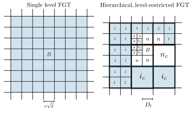
Fig. 2: The original FGT data structure (left) and a level-restricted quad-tree data structure (right). In the original FGT, the interaction region (shaded blue-gray) consists of boxes which are close enough to B𝐵B that the Gaussian field induced by the sources in B𝐵B is significant. (Outside the shaded region, the field is exponentially small and can be ignored for any fixed precision.) In the quad-tree, multiple types of interactions must be accounted for, described in detail in section 4. The interaction list for a typical node B𝐵B consists of the boxes labeled [i𝑖i], while the near neighbors at the same refinement level are labeled [n𝑛n]. For a leaf node B𝐵B, there can be near neighbors at one coarser level [ncsubscript𝑛𝑐n_{c}] or at one finer level [nfsubscript𝑛𝑓n_{f}] as well. The boxes labeled [s𝑠s] are separated from B𝐵B but at a finer level (see Definition 10), while the boxes labeled [icsubscript𝑖𝑐i_{c}] are separated from B𝐵B but at a coarser level (see Definitions 10 and 11).

In the classical FGT [14], aimed at the computation of (14), where the sources are discrete, a uniform grid is superimposed on the computational domain, with a box size of dimension (rδ)dsuperscript𝑟𝛿𝑑(r\sqrt{\delta})^{d}, where r1𝑟1r\approx 1 (Fig. 2, left). Because of the exponential decay of the Gaussian, it is easy to see that only a finite range of nearby boxes need to be considered to achieve any desired precision. That is, the effect due to sources in B𝐵B at targets that are at least m𝑚m boxes away is of the order O(em2r2)𝑂superscript𝑒superscript𝑚2superscript𝑟2O(e^{-m^{2}r^{2}}). Since the field due to sources in any box B𝐵B is efficiently represented by a suitable Hermite expansion (see section 3), it is straightforward to develop an algorithm of complexity O(N+M)𝑂𝑁𝑀O(N+M), where N𝑁N is the number of discrete sources and M𝑀M is the number of targets. The FGT is easily modified to allow for adaptivity. One simply needs to sort the source and target points on the uniform grid while ignoring empty boxes and keeping track of the relevant neighbors for each box. The total storage is then of the order O(N+M)𝑂𝑁𝑀O(N+M) as well. This can be accomplished, for example, with an adaptive quad-tree that is refined uniformly to a level where the box size is approximately (rδ)dsuperscript𝑟𝛿𝑑(r\sqrt{\delta})^{d}, pruning empty boxes on the way.

Such a strategy fails for volume integrals of the form (12), since there are no empty boxes. Instead, we will assume that the right-hand side (the function f𝑓f in (12)) is specified on a level-restricted quad-tree. These data structures have been shown to be extremely effective for elliptic volume integrals [2, 6, 11, 18, 20, 22]. For the sake of simplicity, we assume that the source distribution f𝑓f in (12) is supported in the unit box D𝐷D, centered at the origin. Following the discussion of [11], we assume that superimposed on D𝐷D is a hierarchy of refinements (a quad-tree). Grid level 0 is defined to be D𝐷D itself, with grid level l+1𝑙1l+1 obtained recursively by subdividing each box at level l𝑙l into four equal parts. If B𝐵B is a fixed box at level l𝑙l, the four boxes at level l+1𝑙1l+1 obtained by its subdivision will be referred to as its children. In a level-restricted, adaptive tree, we do not assume the same number of levels is used in all subdomains of D𝐷D. We do, however, require that two leaf nodes which share a boundary point must be no more than one refinement level apart (Fig. 2, right).

On each leaf node B𝐵B, we assume that we are given f𝑓f on a k×k𝑘𝑘k\times k tensor product grid. We may then construct a k𝑘kth-order polynomial approximation to f𝑓f on B𝐵B of the form

fB(y1,y2)j=1NkcB(j)bj(y1,y2),subscript𝑓𝐵subscript𝑦1subscript𝑦2superscriptsubscript𝑗1subscript𝑁𝑘subscript𝑐𝐵𝑗subscript𝑏𝑗subscript𝑦1subscript𝑦2f_{B}(y_{1},y_{2})\approx\sum_{j=1}^{N_{k}}c_{B}(j)\,b_{j}(y_{1},y_{2}), (15)

where Nk=k(k+1)2subscript𝑁𝑘𝑘𝑘12N_{k}=\frac{k(k+1)}{2} is the number of basis functions needed for k𝑘kth order accuracy, and the basis functions bjsubscript𝑏𝑗b_{j} are assumed to be scaled to the relevant box size and centered on the box center. The coefficient vector is defined to be cB=(cB(1),,cB(Nk))subscript𝑐𝐵subscript𝑐𝐵1subscript𝑐𝐵subscript𝑁𝑘\vec{c}_{B}=(c_{B}(1),\dots,c_{B}(N_{k})).

For fourth or sixth order accuracy, one can use as basis functions

{y1ly2m|l,m0,l+mk1}.conditional-setsuperscriptsubscript𝑦1𝑙superscriptsubscript𝑦2𝑚formulae-sequence𝑙𝑚0𝑙𝑚𝑘1\{y_{1}^{l}y_{2}^{m}|\ l,m\geq 0,l+m\leq k-1\}.

If we let fB𝐑k2subscript𝑓𝐵superscript𝐑superscript𝑘2\vec{f_{B}}\in{\bf R}^{k^{2}} denote the given function values (in standard ordering), then the coefficient vector cBsubscript𝑐𝐵\vec{c_{B}} can be computed as the solution of a least squares problem (interpolating the desired data fBsubscript𝑓𝐵\vec{f_{B}} at the corresponding points). The solution operator for this least squares task is denoted by 𝒫𝐑Nk×k2𝒫superscript𝐑subscript𝑁𝑘superscript𝑘2{\cal P}\in{\bf R}^{N_{k}\times k^{2}}, so that

cB=𝒫fB.subscript𝑐𝐵𝒫subscript𝑓𝐵\vec{c}_{B}={\cal P}\,\vec{f_{B}}.

𝒫𝒫{\cal P} can be precomputed and stored (say, using QR factorization). For eighth (or higher) order accuracy, polynomial interpolation is stabilized by assuming that f𝑓f is given on a k×k𝑘𝑘k\times k tensor product Chebyshev grid and using as basis functions

{Tl(y1)Tm(y2)|l,m0,l+mk1},conditional-setsubscript𝑇𝑙subscript𝑦1subscript𝑇𝑚subscript𝑦2formulae-sequence𝑙𝑚0𝑙𝑚𝑘1\{T_{l}(y_{1})T_{m}(y_{2})|\ l,m\geq 0,l+m\leq k-1\},

where Tl(x)subscript𝑇𝑙𝑥T_{l}(x) denotes the (suitably scaled) Chebyshev polynomial of degree l𝑙l. The coefficients of the tensor product Chebyshev expansion can be computed efficiently using the fast cosine transform [4].

In order to develop a fast algorithm for the various kinds of source distributions shown in Fig. 1, we will make use of efficient far field and local representations of the induced field.

3 Analytical apparatus

Following the discussion in [14], we define the Hermite functions hn(x)subscript𝑛𝑥h_{n}(x) by

hn(x)=(1)nDnex2,x,formulae-sequencesubscript𝑛𝑥superscript1𝑛superscript𝐷𝑛superscript𝑒superscript𝑥2𝑥h_{n}(x)=(-1)^{n}D^{n}e^{-x^{2}},\;\;\;x\in{\mathbb{R}},

where D=d/dx𝐷𝑑𝑑𝑥D=d/dx. They satisfy the relation

e(xy)2/δ=n=01n!(yy0δ)nhn(xy0δ),superscript𝑒superscript𝑥𝑦2𝛿superscriptsubscript𝑛01𝑛superscript𝑦subscript𝑦0𝛿𝑛subscript𝑛𝑥subscript𝑦0𝛿e^{-(x-y)^{2}/\delta}=\sum_{n=0}^{\infty}\frac{1}{n!}\left(\frac{y-y_{0}}{\sqrt{\delta}}\right)^{n}h_{n}\left(\frac{x-y_{0}}{\sqrt{\delta}}\right), (16)

where y0subscript𝑦0y_{0}\in{\mathbb{R}} and δ>0𝛿0\delta>0. This formula can be interpreted as an Hermite expansion centered at y0subscript𝑦0y_{0} for the Gaussian field e(xy)2/δsuperscript𝑒superscript𝑥𝑦2𝛿e^{-(x-y)^{2}/\delta} at the target x𝑥x due to the source at y𝑦y. Interchanging x𝑥x and y𝑦y one can also write:

e(xy)2/δ=n=01n!hn(yx0δ)(xx0δ)n.superscript𝑒superscript𝑥𝑦2𝛿superscriptsubscript𝑛01𝑛subscript𝑛𝑦subscript𝑥0𝛿superscript𝑥subscript𝑥0𝛿𝑛e^{-(x-y)^{2}/\delta}=\sum_{n=0}^{\infty}\frac{1}{n!}h_{n}\left(\frac{y-x_{0}}{\sqrt{\delta}}\right)\left(\frac{x-x_{0}}{\sqrt{\delta}}\right)^{n}. (17)

This expresses the Gaussian as a Taylor series in the target location x𝑥x about a center x0subscript𝑥0x_{0}.

It will be convenient to use multi-index notation. In two dimensions, a multi-index is a pair of non-negative integers α=(α1,α2)𝛼subscript𝛼1subscript𝛼2\alpha=(\alpha_{1},\alpha_{2}) with which, for any 𝐱=(x1,x2)𝐑2𝐱subscript𝑥1subscript𝑥2superscript𝐑2{\bf x}=(x_{1},x_{2})\in{\bf R}^{2}, we define:

|α|=α1+α2,α!=α1!α2!,𝐱α=x1α1x2α2,Dα=x1α1x2α2,formulae-sequence𝛼subscript𝛼1subscript𝛼2formulae-sequence𝛼subscript𝛼1subscript𝛼2formulae-sequencesuperscript𝐱𝛼superscriptsubscript𝑥1subscript𝛼1superscriptsubscript𝑥2subscript𝛼2superscript𝐷𝛼superscriptsubscriptsubscript𝑥1subscript𝛼1superscriptsubscriptsubscript𝑥2subscript𝛼2|\alpha|=\alpha_{1}+\alpha_{2},\quad\alpha!=\alpha_{1}!\alpha_{2}!,\quad{\bf x}^{\alpha}=x_{1}^{\alpha_{1}}x_{2}^{\alpha_{2}},\quad D^{\alpha}=\partial_{x_{1}}^{\alpha_{1}}\partial_{x_{2}}^{\alpha_{2}},

If p𝑝p is an integer, we say αp𝛼𝑝\alpha\geq p if α1,α2psubscript𝛼1subscript𝛼2𝑝\alpha_{1},\alpha_{2}\geq p. Multi-dimensional Hermite functions are defined by

hα(𝐱)=hα1(x1)hα2(x2),subscript𝛼𝐱subscriptsubscript𝛼1subscript𝑥1subscriptsubscript𝛼2subscript𝑥2h_{\alpha}({\bf x})=h_{\alpha_{1}}(x_{1})h_{\alpha_{2}}(x_{2}),

and the analogs of (16) and (17) are

e|𝐱𝐲|2/δ=1α!α0(𝐲𝐲0δ)αhα(𝐱𝐲0δ),superscript𝑒superscript𝐱𝐲2𝛿1𝛼subscript𝛼0superscript𝐲subscript𝐲0𝛿𝛼subscript𝛼𝐱subscript𝐲0𝛿e^{-|{\bf x}-{\bf y}|^{2}/\delta}=\frac{1}{\alpha!}\sum_{\alpha\geq 0}\left(\frac{{\bf y}-{\bf y}_{0}}{\sqrt{\delta}}\right)^{\alpha}h_{\alpha}\left(\frac{{\bf x}-{\bf y}_{0}}{\sqrt{\delta}}\right), (18)
e|𝐱𝐲|2/δ=1α!α0hα(𝐲𝐱0δ)(𝐱𝐱0δ)α.superscript𝑒superscript𝐱𝐲2𝛿1𝛼subscript𝛼0subscript𝛼𝐲subscript𝐱0𝛿superscript𝐱subscript𝐱0𝛿𝛼e^{-|{\bf x}-{\bf y}|^{2}/\delta}=\frac{1}{\alpha!}\sum_{\alpha\geq 0}h_{\alpha}\left(\frac{{\bf y}-{\bf x}_{0}}{\sqrt{\delta}}\right)\left(\frac{{\bf x}-{\bf x}_{0}}{\sqrt{\delta}}\right)^{\alpha}. (19)

3.1 Hermite expansions and translation operators

We turn now to the analytical apparatus needed in the FGT algorithm. The first lemma describes how to transform the field due to a volume source distribution and a collection of discrete Gaussians into an Hermite expansion about the center of box B𝐵B in which they are supported.

Lemma 3.

Let B be a box with center 𝐬Bsubscript𝐬𝐵{\bf s}_{B} and side length rδ𝑟𝛿r\sqrt{\delta} and let the Gaussian field ϕ(𝐱)italic-ϕ𝐱\phi({\bf x}) be defined by

ϕ(𝐱)=Be|𝐱𝐲|2δf(𝐲)𝑑𝐲+j=1Nsqje|𝐱𝐲j|2δitalic-ϕ𝐱subscript𝐵superscript𝑒superscript𝐱𝐲2𝛿𝑓𝐲differential-d𝐲superscriptsubscript𝑗1subscript𝑁𝑠subscript𝑞𝑗superscript𝑒superscript𝐱subscript𝐲𝑗2𝛿\phi({\bf x})=\int_{B}e^{-\frac{|{\bf x}-{\bf y}|^{2}}{\delta}}f({\bf y})\,d{\bf y}\ +\sum_{j=1}^{N_{s}}q_{j}e^{-\frac{|{\bf x}-{\bf y}_{j}|^{2}}{\delta}}\, (20)

where the 𝐲jsubscript𝐲𝑗{\bf y}_{j} lie in B. Then,

ϕ(𝐱)=α0Aαhα(𝐱𝐬Bδ),italic-ϕ𝐱subscript𝛼0subscript𝐴𝛼subscript𝛼𝐱subscript𝐬𝐵𝛿\phi({\bf x})=\sum_{\alpha\geq 0}A_{\alpha}h_{\alpha}\left(\frac{{\bf x}-{\bf s}_{B}}{\sqrt{\delta}}\right), (21)

where

Aα=1α!(B(𝐲𝐬Bδ)αf(𝐲)𝑑𝐲+j=1Ns(𝐲j𝐬Bδ)αqj).subscript𝐴𝛼1𝛼subscript𝐵superscript𝐲subscript𝐬𝐵𝛿𝛼𝑓𝐲differential-d𝐲superscriptsubscript𝑗1subscript𝑁𝑠superscriptsubscript𝐲𝑗subscript𝐬𝐵𝛿𝛼subscript𝑞𝑗A_{\alpha}=\frac{1}{\alpha!}\left(\int_{B}\left(\frac{{\bf y}-{\bf s}_{B}}{\sqrt{\delta}}\right)^{\alpha}f({\bf y})\,d{\bf y}+\sum_{j=1}^{N_{s}}\left(\frac{{\bf y}_{j}-{\bf s}_{B}}{\sqrt{\delta}}\right)^{\alpha}q_{j}\right)\,. (22)

The error in truncating the Hermite expansion with p2superscript𝑝2p^{2} terms is given by

|EH(p)|=|αpAαhα(𝐱𝐬Bδ)|K2QB(2Sr(p)+Tr(p))Tr(p),subscript𝐸𝐻𝑝subscript𝛼𝑝subscript𝐴𝛼subscript𝛼𝐱subscript𝐬𝐵𝛿superscript𝐾2subscript𝑄𝐵2subscript𝑆𝑟𝑝subscript𝑇𝑟𝑝subscript𝑇𝑟𝑝|E_{H}(p)|=\left|\sum_{\alpha\geq p}A_{\alpha}h_{\alpha}\left(\frac{{\bf x}-{\bf s}_{B}}{\sqrt{\delta}}\right)\right|\leq K^{2}Q_{B}(2S_{r}(p)+T_{r}(p))T_{r}(p), (23)

where

QB=B|f(𝐲)|𝑑𝐲+j=1Ns|qj|,subscript𝑄𝐵subscript𝐵𝑓𝐲differential-d𝐲superscriptsubscript𝑗1subscript𝑁𝑠subscript𝑞𝑗Q_{B}=\int_{B}|f({\bf y})|d{\bf y}+\sum_{j=1}^{N_{s}}|q_{j}|, (24)
Sr(p)=n=0prnn!,Tr(p)=n=prnn!.formulae-sequencesubscript𝑆𝑟𝑝superscriptsubscript𝑛0𝑝superscript𝑟𝑛𝑛subscript𝑇𝑟𝑝superscriptsubscript𝑛𝑝superscript𝑟𝑛𝑛S_{r}(p)=\sum_{n=0}^{p}\frac{r^{n}}{\sqrt{n!}},\;\;\;T_{r}(p)=\sum_{n=p}^{\infty}\frac{r^{n}}{\sqrt{n!}}. (25)

and K<1.09𝐾1.09K<1.09.

Proof.

The error estimate relies on Cramer’s inequality, which takes the form

1α!|hα(𝐱)|K22|α|/21α!e|𝐱|2/21𝛼subscript𝛼𝐱superscript𝐾2superscript2𝛼21𝛼superscript𝑒superscript𝐱22\frac{1}{\alpha!}|h_{\alpha}({\bf x})|\leq K^{2}2^{|\alpha|/2}\frac{1}{\sqrt{\alpha!}}e^{-|{\bf x}|^{2}/2} (26)

in two dimensions, where K<1.09𝐾1.09K<1.09, and the fact that

|𝐲𝐬Bδ|22r,𝐲subscript𝐬𝐵𝛿22𝑟\left|\frac{{\bf y}-{\bf s}_{B}}{\sqrt{\delta}}\right|\leq\frac{\sqrt{2}}{2}r, (27)

for 𝐲𝐲{\bf y} in B𝐵B. The desired result follows from integration over the domain B𝐵B and summation over the discrete sources. \Box

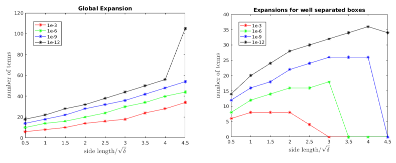
Note that the Hermite expansion converges extremely rapidly for r<1𝑟1r<1. For larger r𝑟r, they still converge but require larger values of p𝑝p. (See [3, 19, 26, 31] for further discussion of error estimates.) In the original FGT, setting r1𝑟1r\approx 1 is a sensible choice, since a modest value of p𝑝p is sufficient and the number of boxes within the interaction region (where the Gaussian field is not vanishingly small) is modest as well. The interaction region for a box B𝐵B is the shaded area on the left in Fig. 2. A second thing to note is that the estimate is uniform with respect to the target. In the original FGT, this is necessary since the Hermite expansion is evaluated at all relevant locations. In the hierarchical FGT, however, the Gaussian field due to an Hermite expansion is evaluated only for boxes that are “well-separated” (the boxes labeled by i𝑖i on the right-hand side of Fig. 2). Moreover, we will compute such interactions at every level of the quad-tree, so that the boxes could be of arbitrary size. Fortunately, once boxes are separated by a distance Rδ𝑅𝛿R\sqrt{\delta}, their interactions can be ignored with an error of the order O(eR2)𝑂superscript𝑒superscript𝑅2O(e^{-R^{2}}), limiting the size of the expansions (see Fig. 3).
Refer to caption
Fig. 3: (Left) plot of the number of terms p𝑝p needed in an Hermite expansion as a function of the box size, when used uniformly in the plane, including the near field. (Right) plot of the number of terms needed when used only in the far field.

In the full algorithm, a more refined estimate that makes use of the separation criterion will be useful. We have the following lemma.

Lemma 4.

Let B𝐵B be a box with center 𝐬Bsubscript𝐬𝐵{\bf s}_{B} and side length rδ𝑟𝛿r\sqrt{\delta}, and let C𝐶C be a box with center 𝐭Csubscript𝐭𝐶{\bf t}_{C} and side length rδ𝑟𝛿r\sqrt{\delta} with xC𝑥𝐶x\in C. Assuming the distance between B and C is at least rδ𝑟𝛿r\sqrt{\delta}, the Gaussian field defined by (20) and its Hermite expansion (21) satisfy the error bound:

|EH(p)|=|αpAαhα(𝐱𝐬Bδ)|=K2QBe98r2(2Sr(p)+Tr(p))Tr(p),subscript𝐸𝐻𝑝subscript𝛼𝑝subscript𝐴𝛼subscript𝛼𝐱subscript𝐬𝐵𝛿superscript𝐾2subscript𝑄𝐵superscript𝑒98superscript𝑟22subscript𝑆𝑟𝑝subscript𝑇𝑟𝑝subscript𝑇𝑟𝑝|E_{H}(p)|=\left|\sum_{\alpha\geq p}A_{\alpha}h_{\alpha}\left(\frac{{\bf x}-{\bf s}_{B}}{\sqrt{\delta}}\right)\right|=K^{2}Q_{B}e^{-\frac{9}{8}r^{2}}(2S_{r}(p)+T_{r}(p))T_{r}(p), (28)

where QBsubscript𝑄𝐵Q_{B} is given by (24), and Sr(p)subscript𝑆𝑟𝑝S_{r}(p), Tr(p)subscript𝑇𝑟𝑝T_{r}(p) are given by (25).

Proof.

The proof follows the same outline as that of Lemma 3. In this case, after applying Cramer’s inequality (26), we make the additional observation that |𝐱𝐬Bδ|32r𝐱subscript𝐬𝐵𝛿32𝑟|\frac{{\bf x}-{\bf s}_{B}}{\sqrt{\delta}}|\geq\frac{3}{2}r, which contributes to the exponential decay in r𝑟r. \Box

The next lemma describes the conversion of an Hermite expansion about 𝐬Bsubscript𝐬𝐵{\bf s}_{B} into a Taylor expansion about 𝐭Csubscript𝐭𝐶{\bf t}_{C}.

Lemma 5.

Let

ϕ(𝐱)=α0Aαhα(𝐱𝐬Bδ),italic-ϕ𝐱subscript𝛼0subscript𝐴𝛼subscript𝛼𝐱subscript𝐬𝐵𝛿\phi({\bf x})=\sum_{\alpha\geq 0}A_{\alpha}h_{\alpha}\left(\frac{{\bf x}-{\bf s}_{B}}{\sqrt{\delta}}\right), (29)

denote the Hermite expansion of a Gaussian field induced by a source distribution in a box B𝐵B with center 𝐬Bsubscript𝐬𝐵{\bf s}_{B} and side length rδ𝑟𝛿r\sqrt{\delta}. Then ϕ(𝐱)italic-ϕ𝐱\phi({\bf x}) has the following Taylor expansion about the center 𝐭Csubscript𝐭𝐶{\bf t}_{C} of box C𝐶C with side length rδ𝑟𝛿r\sqrt{\delta}:

ϕ(𝐱)=β0Bβ(𝐱𝐭Cδ)β.italic-ϕ𝐱subscript𝛽0subscript𝐵𝛽superscript𝐱subscript𝐭𝐶𝛿𝛽\phi({\bf x})=\sum_{\beta\geq 0}B_{\beta}\left(\frac{{\bf x}-{\bf t}_{C}}{\sqrt{\delta}}\right)^{\beta}. (30)

The coefficients are given by

Bβ=(1)|β|β!α0Aαhα+β(𝐬B𝐭Cδ).subscript𝐵𝛽superscript1𝛽𝛽subscript𝛼0subscript𝐴𝛼subscript𝛼𝛽subscript𝐬𝐵subscript𝐭𝐶𝛿B_{\beta}=\frac{(-1)^{|\beta|}}{\beta!}\sum_{\alpha\geq 0}A_{\alpha}h_{\alpha+\beta}\left(\frac{{\bf s}_{B}-{\bf t}_{C}}{\sqrt{\delta}}\right). (31)

Assuming that the distance between boxes B𝐵B and C𝐶C is at least rδ𝑟𝛿r\sqrt{\delta}, the error ET(p)subscript𝐸𝑇𝑝E_{T}(p) in truncating the Taylor series after p2superscript𝑝2p^{2} terms satisfies

|ET(p)|=|αpAαhα(𝐱𝐬Bδ)|K2QBe98r2(2Sr(p)+Tr(p))Tr(p),subscript𝐸𝑇𝑝subscript𝛼𝑝subscript𝐴𝛼subscript𝛼𝐱subscript𝐬𝐵𝛿superscript𝐾2subscript𝑄𝐵superscript𝑒98superscript𝑟22subscript𝑆𝑟𝑝subscript𝑇𝑟𝑝subscript𝑇𝑟𝑝|E_{T}(p)|=\left|\sum_{\alpha\geq p}A_{\alpha}h_{\alpha}\left(\frac{{\bf x}-{\bf s}_{B}}{\sqrt{\delta}}\right)\right|\leq K^{2}Q_{B}e^{-\frac{9}{8}r^{2}}(2S_{r}(p)+T_{r}(p))T_{r}(p), (32)

where QBsubscript𝑄𝐵Q_{B} is given by (24), and Sr(p)subscript𝑆𝑟𝑝S_{r}(p), Tr(p)subscript𝑇𝑟𝑝T_{r}(p) are given by (25).

Proof.

This result follows, again, from the standard error estimate in [3, 26, 31], with one modification; the exponential term in Cramer’s inequality can be bounded by e98r2superscript𝑒98superscript𝑟2e^{-\frac{9}{8}r^{2}}, instead of 1. \Box

In practice, we need a variant of Lemma 5, in which the Hermite expansion is truncated before being converted to a Taylor expansion.

Lemma 6.

Let

ϕ(𝐱)=αpAαhα(𝐱𝐬Bδ)italic-ϕ𝐱subscript𝛼𝑝subscript𝐴𝛼subscript𝛼𝐱subscript𝐬𝐵𝛿\phi({\bf x})=\sum_{\alpha\leq p}A_{\alpha}h_{\alpha}\left(\frac{{\bf x}-{\bf s}_{B}}{\sqrt{\delta}}\right) (33)

denote a truncated Hermite expansion corresponding to the Gaussian field induced by a source distribution in a box B𝐵B with center 𝐬Bsubscript𝐬𝐵{\bf s}_{B} and side length rδ𝑟𝛿r\sqrt{\delta}. The induced Taylor series in a box C𝐶C with center 𝐭Csubscript𝐭𝐶{\bf t}_{C} and side length rδ𝑟𝛿r\sqrt{\delta} is given by

ϕ(𝐱)=β0Cβ(𝐱𝐭Cδ)β,italic-ϕ𝐱subscript𝛽0subscript𝐶𝛽superscript𝐱subscript𝐭𝐶𝛿𝛽\phi({\bf x})=\sum_{\beta\geq 0}C_{\beta}\left(\frac{{\bf x}-{\bf t}_{C}}{\sqrt{\delta}}\right)^{\beta}, (34)

with coefficients

Cβ=(1)|β|β!αpAαhα+β(𝐬B𝐭Cδ).subscript𝐶𝛽superscript1𝛽𝛽subscript𝛼𝑝subscript𝐴𝛼subscript𝛼𝛽subscript𝐬𝐵subscript𝐭𝐶𝛿C_{\beta}=\frac{(-1)^{|\beta|}}{\beta!}\sum_{\alpha\leq p}A_{\alpha}h_{\alpha+\beta}\left(\frac{{\bf s}_{B}-{\bf t}_{C}}{\sqrt{\delta}}\right). (35)

Assuming that the distance between boxes B𝐵B and C𝐶C is at least rδ𝑟𝛿r\sqrt{\delta}, the error EHT(p)subscript𝐸𝐻𝑇𝑝E_{HT}(p) in truncating the Taylor series after p2superscript𝑝2p^{2} terms satisfies the bound

|EHT(p)|=|αpAαhα(𝐱𝐬Bδ)|K2QBe2r2(2Sr(p)+Tr(p))Tr(p)Sr2(p),subscript𝐸𝐻𝑇𝑝subscript𝛼𝑝subscript𝐴𝛼subscript𝛼𝐱subscript𝐬𝐵𝛿superscript𝐾2subscript𝑄𝐵superscript𝑒2superscript𝑟22subscript𝑆𝑟𝑝subscript𝑇𝑟𝑝subscript𝑇𝑟𝑝superscriptsubscript𝑆𝑟2𝑝|E_{HT}(p)|=\left|\sum_{\alpha\geq p}A_{\alpha}h_{\alpha}\left(\frac{{\bf x}-{\bf s}_{B}}{\sqrt{\delta}}\right)\right|\leq K^{2}Q_{B}e^{-2r^{2}}(2S_{r}(p)+T_{r}(p))T_{r}(p)S_{r}^{2}(p), (36)

where QBsubscript𝑄𝐵Q_{B} is given by (24), and Sr(p)subscript𝑆𝑟𝑝S_{r}(p), Tr(p)subscript𝑇𝑟𝑝T_{r}(p) are given by (25).

Proof.

The result is a straightforward application of the triangle inequality and Lemma 5. \Box

Note that the total error in using both an Hermite and a local expansion consists of two contributions: the first comes from truncating the Hermite expansion, given by (23), while the second comes from truncating the local expansion, according to (36).

For the hierarchical FGT, we will also need to propagate Hermite and Taylor expansions between levels of the quad-tree. The following two lemmas provide the needed analytical tools. Lemma 7 describes a formula for shifting the center of an Hermite expansion, and Lemma 8 describes one for shifting the center of a Taylor expansion. The derivation is straightforward [19].

Lemma 7.

Let a Gaussian field be given by the Hermite expansion

ϕ(𝐱)=α0Aαhα(𝐱𝐬Bδ),italic-ϕ𝐱subscript𝛼0subscript𝐴𝛼subscript𝛼𝐱subscript𝐬𝐵𝛿\phi({\bf x})=\sum_{\alpha\geq 0}A_{\alpha}h_{\alpha}\left(\frac{{\bf x}-{\bf s}_{B}}{\sqrt{\delta}}\right), (37)

about a center 𝐬Bsubscript𝐬𝐵{\bf s}_{B} and let 𝐬Csubscript𝐬𝐶{\bf s}_{C} denoted a shifted expansion center. Then,

ϕ(𝐱)=β0Bβhβ(𝐱𝐬Cδ),italic-ϕ𝐱subscript𝛽0subscript𝐵𝛽subscript𝛽𝐱subscript𝐬𝐶𝛿\phi({\bf x})=\sum_{\beta\geq 0}B_{\beta}h_{\beta}\left(\frac{{\bf x}-{\bf s}_{C}}{\sqrt{\delta}}\right), (38)

where the coefficients are given by:

Bβ=αβα!β!(βα)(𝐬B𝐬Cδ)βαAα.subscript𝐵𝛽subscript𝛼𝛽𝛼𝛽binomial𝛽𝛼superscriptsubscript𝐬𝐵subscript𝐬𝐶𝛿𝛽𝛼subscript𝐴𝛼B_{\beta}=\sum_{\alpha\leq\beta}\frac{\alpha!}{\beta!}\binom{\beta}{\alpha}\left(\frac{{\bf s}_{B}-{\bf s}_{C}}{\sqrt{\delta}}\right)^{\beta-\alpha}A_{\alpha}. (39)
Lemma 8.

Let 𝐭B2subscript𝐭𝐵superscript2{\bf t}_{B}\in{\mathbb{R}}^{2} and let {Cα}subscript𝐶𝛼\{C_{\alpha}\} denote the expansion coefficients for a truncated Taylor series with p2superscript𝑝2p^{2} terms. Letting 𝐭C2subscript𝐭𝐶superscript2{\bf t}_{C}\in{\mathbb{R}}^{2} be a shifted expansion center, we have

αpCα(𝐱𝐭Bδ)α=βpCβ(𝐱𝐭Cδ)β,subscript𝛼𝑝subscript𝐶𝛼superscript𝐱subscript𝐭𝐵𝛿𝛼subscript𝛽𝑝subscriptsuperscript𝐶𝛽superscript𝐱subscript𝐭𝐶𝛿𝛽\sum_{\alpha\leq p}C_{\alpha}\left(\frac{{\bf x}-{\bf t}_{B}}{\sqrt{\delta}}\right)^{\alpha}=\sum_{\beta\leq p}C^{\prime}_{\beta}\left(\frac{{\bf x}-{\bf t}_{C}}{\sqrt{\delta}}\right)^{\beta}, (40)

where

Cβ=βαpCα(αβ)(𝐭C𝐭Bδ)αβ.subscriptsuperscript𝐶𝛽subscript𝛽𝛼𝑝subscript𝐶𝛼binomial𝛼𝛽superscriptsubscript𝐭𝐶subscript𝐭𝐵𝛿𝛼𝛽C^{\prime}_{\beta}=\sum_{\beta\leq\alpha\leq p}C_{\alpha}\binom{\alpha}{\beta}\left(\frac{{\bf t}_{C}-{\bf t}_{B}}{\sqrt{\delta}}\right)^{\alpha-\beta}\,. (41)

3.2 Local interactions

In the previous section, we summarized the analytical machinery needed for the fast evaluation of Gaussian fields with well separated sources and targets. Before providing a formal description of the full algorithm in the next section, it remains to consider the computation of local interactions between neighboring boxes at the level of leaf nodes. For point sources, this is done by direct evaluation. We concentrate in this section on domain integrals, and defer a discussion of densities supported on boundaries to section 4.2.
Refer to caption
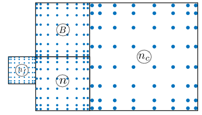
Fig. 4: For a leaf node B𝐵B, there are three types of possible local interactions: the interaction with a colleague (a neighbor at the same refinement level, including the self-interaction), and the interaction with fine and coarse neighbors - one level finer or one level coarser, respectively. The grid shown corresponds to an 8th𝑡th order accurate tensor product Chebyshev discretization.

Thus, suppose B𝐵B is a leaf node - that is a box at level l𝑙l of the tree hierarchy on which a k×k𝑘𝑘k\times k tensor product grid of function values has been specified. Let rlsubscript𝑟𝑙r_{l} denote the side length of B𝐵B, so that its area is rl×rlsubscript𝑟𝑙subscript𝑟𝑙r_{l}\times r_{l}. Consider now a target point 𝐭𝐭{\bf t}, which lies in either B𝐵B, a neighboring box of B𝐵B at the same refinement level, or a coarse or fine neighbor for B𝐵B, which can be at most one refinement level apart. Because of the translation invariance of the kernel, a simple counting argument shows that there are at most k×k×9𝑘𝑘9k\times k\times 9 possible targets at the same level and at most k×k×12𝑘𝑘12k\times k\times 12 possible targets in neighbors at either a coarser or finer level. Recalling that the source distribution f𝑓f on B𝐵B is given by (15), the Gaussian field induced at 𝐭𝐭{\bf t} by fBsubscript𝑓𝐵f_{B} can be approximated by

ψB(𝐭)=n=1NkcB(n)G(𝐭,n),subscript𝜓𝐵𝐭superscriptsubscript𝑛1subscript𝑁𝑘subscript𝑐𝐵𝑛𝐺𝐭𝑛\psi_{B}({\bf t})=\sum_{n=1}^{N_{k}}c_{B}(n)G({\bf t},n), (42)

with

G(𝐭,n)=Be(t1y1)2δe(t2y2)2δbn(y1,y2)𝑑y1𝑑y2,𝐺𝐭𝑛subscript𝐵superscript𝑒superscriptsubscript𝑡1subscript𝑦12𝛿superscript𝑒superscriptsubscript𝑡2subscript𝑦22𝛿subscript𝑏𝑛subscript𝑦1subscript𝑦2differential-dsubscript𝑦1differential-dsubscript𝑦2G({\bf t},n)=\int_{B}e^{-\frac{(t_{1}-y_{1})^{2}}{\delta}}e^{-\frac{(t_{2}-y_{2})^{2}}{\delta}}b_{n}(y_{1},y_{2})\,dy_{1}dy_{2}, (43)

where (t1,t2)subscript𝑡1subscript𝑡2(t_{1},t_{2}), (y1,y2)subscript𝑦1subscript𝑦2(y_{1},y_{2}) denote the coordinates of the target 𝐭𝐭{\bf t} and source with respect to the center of box B𝐵B. Once the values {G(𝐭,n)}𝐺𝐭𝑛\{G({\bf t},n)\} have been tabulated for all possible target locations and all basis functions, all local interactions can be computed directly from (42), with some care in bookkeeping.

Assuming bn(y1,y2)=pn1(y1)pn2(y2)subscript𝑏𝑛subscript𝑦1subscript𝑦2subscript𝑝subscript𝑛1subscript𝑦1subscript𝑝subscript𝑛2subscript𝑦2b_{n}(y_{1},y_{2})=p_{n_{1}}(y_{1})p_{n_{2}}(y_{2}), the formula for G(𝐭,n)𝐺𝐭𝑛G({\bf t},n) can be written in the form

G(𝐭,n)=rl/2rl/2e(t1y1)2δpn1(y1)𝑑y1rl/2rl/2e(t2y2)2δpn2(y2)𝑑y2.𝐺𝐭𝑛superscriptsubscriptsubscript𝑟𝑙2subscript𝑟𝑙2superscript𝑒superscriptsubscript𝑡1subscript𝑦12𝛿subscript𝑝subscript𝑛1subscript𝑦1differential-dsubscript𝑦1superscriptsubscriptsubscript𝑟𝑙2subscript𝑟𝑙2superscript𝑒superscriptsubscript𝑡2subscript𝑦22𝛿subscript𝑝subscript𝑛2subscript𝑦2differential-dsubscript𝑦2G({\bf t},n)=\int_{-r_{l}/2}^{r_{l}/2}e^{-\frac{(t_{1}-y_{1})^{2}}{\delta}}p_{n_{1}}(y_{1})dy_{1}\cdot\int_{-r_{l}/2}^{r_{l}/2}e^{-\frac{(t_{2}-y_{2})^{2}}{\delta}}p_{n_{2}}(y_{2})dy_{2}. (44)

Thus, for colleagues (boxes at the same refinement level), there are at most 3k3𝑘3k possible relative target locations (tiyi)subscript𝑡𝑖subscript𝑦𝑖(t_{i}-y_{i}) and at most k𝑘k basis functions pni(yi)subscript𝑝subscript𝑛𝑖subscript𝑦𝑖p_{n_{i}}(y_{i}), which are either monomials or scaled Chebyshev polynomials. These 3k23superscript𝑘23k^{2} numbers can be computed in milliseconds on a single core. For coarse or fine colleagues, it is straightfoward to check that there are at most 4k4𝑘4k possible relative target locations (tiyi)subscript𝑡𝑖subscript𝑦𝑖(t_{i}-y_{i}), so that these tables involving 4k24superscript𝑘24k^{2} numbers can be generated in milliseconds as well. Finally, we note that such tables must be generated for each refinement level that contains a leaf node.

4 FGT algorithm

We now describe an adaptive version of the Fast Gauss Transform, closely following the discussion in [11]. Since the Gaussian kernel e𝐱𝐲2/δsuperscript𝑒superscriptnorm𝐱𝐲2𝛿e^{-\|{\bf x}-{\bf y}\|^{2}/\delta} is rapidly decaying, we will ignore interactions beyond a distance where they can be considered negligible, according to a user-defined precision ϵitalic-ϵ\epsilon. That is, we define a cut-off parameter rcsubscript𝑟𝑐r_{c} so that e|𝐱𝐲|2/δϵsuperscript𝑒superscript𝐱𝐲2𝛿italic-ϵe^{-|{\bf x}-{\bf y}|^{2}/\delta}\leq\epsilon, when 𝐱𝐲rcδnorm𝐱𝐲subscript𝑟𝑐𝛿\|{\bf x}-{\bf y}\|\geq r_{c}\sqrt{\delta}. Clearly, if a source box has side length greater than or equal to rcδsubscript𝑟𝑐𝛿r_{c}\sqrt{\delta}, its contribution to well-separated boxes is negligible. We will also make use of the following definitions:

Definition 9.

(Cutoff level): Given a quad-tree with levels l=0,1,,L𝑙01𝐿l=0,1,\cdots,L, the cutoff level is defined to be the coarsest level of the tree at which the box size is smaller than or equal to rcδsubscript𝑟𝑐𝛿r_{c}\sqrt{\delta}. We denote this by lcutsubscript𝑙𝑐𝑢𝑡l_{cut}. If the box size is greater than rcδsubscript𝑟𝑐𝛿r_{c}\sqrt{\delta} even at the finest level (level L𝐿L), we let lcut=L+1subscript𝑙𝑐𝑢𝑡𝐿1l_{cut}=L+1.

Definition 10.

(Neighbors): Leaf nodes at the same level as B𝐵B which share a boundary point, including B𝐵B itself, are referred to as colleagues. Leaf nodes at the level of B𝐵B’s parent which share a boundary point with B𝐵B are referred to as the coarse neighbors of B𝐵B. Leaf nodes one level finer than B𝐵B which share a boundary point with B𝐵B are referred to as fine neighbors. Together, the union of the colleagues, coarse neighbors and fine neighbors of B𝐵B are referred to as B𝐵B’s neighbors. The s-list of a box B𝐵B consists of those children of B𝐵B’s colleagues which are not fine neighbors of B𝐵B (Fig. 2).

Definition 11.

(Interaction lists): The interaction region for B𝐵B consists of the area covered by the neighbors of B𝐵B’s parent, excluding the area covered by B𝐵B’s colleagues and coarse neighbors. The interaction list for B𝐵B consists of those boxes in the interaction region which are at the same refinement level (marked i𝑖i in Fig.2), and is denoted by (B)𝐵{\cal I}(B). Boxes at coarser levels will be referred to as the coarse interaction list, denoted by c(B)subscript𝑐𝐵{\cal I}_{c}(B) (marked icsubscript𝑖𝑐i_{c} in Fig.2).

Definition 12.

(Expansions): We denote by Bl,ksubscript𝐵𝑙𝑘B_{l,k} the kth box at refinement level l𝑙l and by Φl,ksubscriptΦ𝑙𝑘\Phi_{l,k} the Hermite expansion describing the far field due to the source distribution supported inside Bl,ksubscript𝐵𝑙𝑘B_{l,k}. We denote by Ψl,ksubscriptΨ𝑙𝑘\Psi_{l,k} the local expansion describing the field due to the source distribution outside the neighbors of Bl,ksubscript𝐵𝑙𝑘B_{l,k} and by Ψ~l,ksubscript~Ψ𝑙𝑘\tilde{\Psi}_{l,k} the local expansion describing the field due to the source distribution outside the neighbors of the parent of Bl,ksubscript𝐵𝑙𝑘B_{l,k}. When the context is clear, we will sometimes use the notation Φ(B)Φ𝐵\Phi(B), Ψ(B)Ψ𝐵\Psi(B), Ψ~(B)~Ψ𝐵\tilde{\Psi}(B) to describe the expansions associated with a box B𝐵B.

Remark 1.

Let B=Bl,k𝐵subscript𝐵𝑙𝑘B=B_{l,k} be a box in the quad-tree hierarchy with children C1,C2,C3,C4subscript𝐶1subscript𝐶2subscript𝐶3subscript𝐶4C_{1},C_{2},C_{3},C_{4}. Then, according to Lemma 7, there is a linear operator 𝒯HHsubscript𝒯𝐻𝐻{\cal T}_{HH} for which

Φl,k=Φ(B)=𝒯HH[Φ(C1),Φ(C2),Φ(C3),Φ(C4)].subscriptΦ𝑙𝑘Φ𝐵subscript𝒯𝐻𝐻Φsubscript𝐶1Φsubscript𝐶2Φsubscript𝐶3Φsubscript𝐶4\Phi_{l,k}=\Phi(B)={\cal T}_{HH}[\Phi(C_{1}),\Phi(C_{2}),\Phi(C_{3}),\Phi(C_{4})]. (45)

The operator 𝒯HHsubscript𝒯𝐻𝐻{\cal T}_{HH} is responsible for merging the expansions of four children into a single expansion for the parent. Likewise, according to Lemma 8 there is a linear operator 𝒯LLsubscript𝒯𝐿𝐿{\cal T}_{LL} for which

[Ψ~(C1),Ψ~(C2),Ψ~(C3),Ψ~(C4)]=𝒯LLΨl,k=𝒯LLΨ(B).~Ψsubscript𝐶1~Ψsubscript𝐶2~Ψsubscript𝐶3~Ψsubscript𝐶4subscript𝒯𝐿𝐿subscriptΨ𝑙𝑘subscript𝒯𝐿𝐿Ψ𝐵[\tilde{\Psi}(C_{1}),\tilde{\Psi}(C_{2}),\tilde{\Psi}(C_{3}),\tilde{\Psi}(C_{4})]={\cal T}_{LL}\,\Psi_{l,k}={\cal T}_{LL}\,\Psi(B). (46)

𝒯LLsubscript𝒯𝐿𝐿{\cal T}_{LL} is responsible for shifting the incoming data (the local expansion) from a parent box to its children. Finally, according to Lemma 6, for any source box Bl,ksubscript𝐵superscript𝑙superscript𝑘B_{l^{\prime},k^{\prime}} in the interaction list (B)𝐵{\cal I}(B) of box Bl,ksubscript𝐵𝑙𝑘B_{l,k}, there is a linear operator 𝒯HLsubscript𝒯𝐻𝐿{\cal T}_{HL} for which the induced field in Bl,ksubscript𝐵𝑙𝑘B_{l,k} is given by Ψ=THLΦl,kΨsubscript𝑇𝐻𝐿subscriptΦsuperscript𝑙superscript𝑘\Psi=T_{HL}\Phi_{l^{\prime},k^{\prime}}. Clearly,

Ψl,k=Ψ~l,k+i(B)THLΦi.subscriptΨ𝑙𝑘subscript~Ψ𝑙𝑘subscript𝑖𝐵subscript𝑇𝐻𝐿subscriptΦ𝑖\Psi_{l,k}=\tilde{\Psi}_{l,k}+\sum_{i\in{\cal I}(B)}T_{HL}\Phi_{i}. (47)

Since our adaptive algorithm is operating on a level-restricted adaptive tree, the leaf nodes need to handle far field interactions between boxes at different levels. More precisely, viewing each such leaf node B𝐵B as a “target box”, we need to incorporate the influence of the s-list and the coarse interaction list (see Fig. 2). For every box in the s-list, its Hermite expansion is rapidly convergent in B𝐵B and its influence can be computed by direct evaluation of the series. We also need to compute the dual interaction - namely the influence of a leaf node B𝐵B on a box Bsuperscript𝐵B^{\prime} in the s-list. Rather than evaluate the Hermite expansion of B𝐵B at all targets in Bsuperscript𝐵B^{\prime}, or shifting to a local expansion in Bsuperscript𝐵B^{\prime}, we can directly expand the influence of the polynomial source distribution in B𝐵B, given by the coefficients cBsubscript𝑐𝐵\vec{c}_{B}, as a local expansion in Bsuperscript𝐵B^{\prime}. Thus, incorporating all far field interactions into (47), we have:

Ψl,k=Ψ~l,k+iTHLΦi,+icTdirectci.subscriptΨ𝑙𝑘subscript~Ψ𝑙𝑘subscript𝑖subscript𝑇𝐻𝐿subscriptΦ𝑖subscript𝑖subscript𝑐subscript𝑇𝑑𝑖𝑟𝑒𝑐𝑡subscript𝑐𝑖\Psi_{l,k}=\tilde{\Psi}_{l,k}+\sum_{i\in{\cal I}}T_{HL}\Phi_{i},+\sum_{i\in{\cal I}_{c}}T_{direct}\,\vec{c}_{i}. (48)

The operator Tdirectsubscript𝑇𝑑𝑖𝑟𝑒𝑐𝑡T_{direct}, which maps the coefficients of a polynomial approximation of the density in Bsuperscript𝐵B^{\prime} (a coarse interaction list box) onto the p2superscript𝑝2p^{2} coefficients of the local expansion in B𝐵B can be precomputed and stored for each level in the quad-tree hierarchy. Inspection of Fig. 2, the translation invariance of the kernel, and a simple counting argument show that this requires O(kpL)𝑂𝑘𝑝𝐿O(kpL) work and storage, where k𝑘k is the order of polynomial approximation, p𝑝p is the order of the local expansion, and L𝐿L is the number of levels. More precisely, let bn(y1,y2)=pn1(y1)pn2(y2)subscript𝑏𝑛subscript𝑦1subscript𝑦2subscript𝑝subscript𝑛1subscript𝑦1subscript𝑝subscript𝑛2subscript𝑦2b_{n}(y_{1},y_{2})=p_{n_{1}}(y_{1})\,p_{n_{2}}(y_{2}) be a basis function for the polynomial approximation in box Bsuperscript𝐵B^{\prime} and let α=(α1,α2)𝛼subscript𝛼1subscript𝛼2\alpha=(\alpha_{1},\alpha_{2}) denote the multi-index of a term in the induced local expansion in B𝐵B. Then

Tdirect(α,n)=T1(α1,n1)T2(α2,n2),subscript𝑇𝑑𝑖𝑟𝑒𝑐𝑡𝛼𝑛subscript𝑇1subscript𝛼1subscript𝑛1subscript𝑇2subscript𝛼2subscript𝑛2T_{direct}(\alpha,n)=T_{1}(\alpha_{1},n_{1})\,T_{2}(\alpha_{2},n_{2}), (49)

where

Ti(αi,ni)=1αi!Dl1/2Dl1/2hαi(yisiδ)pni(yi)𝑑yi,subscript𝑇𝑖subscript𝛼𝑖subscript𝑛𝑖1subscript𝛼𝑖superscriptsubscriptsubscript𝐷𝑙12subscript𝐷𝑙12subscriptsubscript𝛼𝑖subscript𝑦𝑖subscript𝑠𝑖𝛿subscript𝑝subscript𝑛𝑖subscript𝑦𝑖differential-dsubscript𝑦𝑖T_{i}(\alpha_{i},n_{i})=\frac{1}{\alpha_{i}!}\int_{D_{l-1}/2}^{D_{l-1}/2}h_{\alpha_{i}}\left(\frac{y_{i}-s_{i}}{\sqrt{\delta}}\right)p_{n_{i}}(y_{i})\,dy_{i}\,,

(s1,s2)subscript𝑠1subscript𝑠2(s_{1},s_{2}) denotes the center of B𝐵B, and Dl1subscript𝐷𝑙1D_{l-1} denotes the side length of box Bsuperscript𝐵B^{\prime} at level l1𝑙1l-1.

4.1 Pseudocode for the FGT

We assume we are given a square domain B0,0subscript𝐵00B_{0,0}, on which is superimposed an adaptive hierarchical quad-tree with lmaxsubscript𝑙𝑚𝑎𝑥l_{max} refinement levels. We let lcutsubscript𝑙𝑐𝑢𝑡l_{cut} denote the cutoff level. If lcutlmaxsubscript𝑙𝑐𝑢𝑡subscript𝑙𝑚𝑎𝑥l_{cut}\leq l_{max}, for each level l that satisfies the condition lcutllmaxsubscript𝑙𝑐𝑢𝑡𝑙subscript𝑙𝑚𝑎𝑥l_{cut}\leq l\leq l_{max}, determine the number of terms needed in the Hermite expansions Nh(l)subscript𝑁𝑙N_{h}(l) and the number of terms needed in the local expansion Nt(l)subscript𝑁𝑡𝑙N_{t}(l) according to the box size, the parameter δ𝛿\delta that defines the variance of the Gaussian, the user-defined precision ϵitalic-ϵ\epsilon, and the estimates (28), (32).

We denote the leaf nodes by Bi,i=1,,Mformulae-sequencesubscript𝐵𝑖𝑖1𝑀B_{i},\ i=1,\dots,M, where M𝑀M is the total number of leaf nodes across all levels. We assume that the source distribution on each Bisubscript𝐵𝑖B_{i} is given by a collection of point sources, as well as a smooth function f𝑓f, sampled on a k×k𝑘𝑘k\times k grid. The number of grid points is denoted by N=Mk2𝑁𝑀superscript𝑘2N=Mk^{2} and the number of discrete sources is denoted by Nssubscript𝑁𝑠N_{s}. We assume the output is desired at the N𝑁N grid points as well as the Nssubscript𝑁𝑠N_{s} source locations.

Step I: Upward pass

for l=lmax,,lcut𝑙subscript𝑙𝑚𝑎𝑥subscript𝑙𝑐𝑢𝑡l=l_{max},\dots,l_{cut}
for every box j𝑗j on level l𝑙l
if j𝑗j is childless then
\bullet Form Hermite expansion Φl,jsubscriptΦ𝑙𝑗\Phi_{l,j} using (22)
else
\bullet Form Hermite expansion Φl,jsubscriptΦ𝑙𝑗\Phi_{l,j} by merging the expansions of
     its children using 𝒯HHsubscript𝒯𝐻𝐻{\cal T}_{HH} (see Lemma 7)
endif
end
end

Step II: Downward pass

for every box j𝑗j on level lcutsubscript𝑙𝑐𝑢𝑡l_{cut}
\bullet Set Ψlcut,j=0subscriptΨsubscript𝑙𝑐𝑢𝑡𝑗0\Psi_{l_{cut},j}=0
end
for l=lcut+1,,lmax𝑙subscript𝑙𝑐𝑢𝑡1subscript𝑙𝑚𝑎𝑥l=l_{cut}+1,\dots,l_{max}
for every box j𝑗j on level l𝑙l:
\bullet Compute Ψ~l,jsubscript~Ψ𝑙𝑗\tilde{\Psi}_{l,j} from its parent’s ΨΨ\Psi expansion using the operator
     𝒯LLsubscript𝒯𝐿𝐿{\cal T}_{LL}
for every box m𝑚m in j𝑗j’s interaction list:
\bullet Increment Ψl,jsubscriptΨ𝑙𝑗\Psi_{l,j} by adding in the contributions from all boxes
     in j𝑗j’s interaction list, using (48).
if j𝑗j is childless then
for every box m𝑚m in j𝑗j’s s-list:
\bullet Evaluate the Hermite expansion Φ(m)Φ𝑚\Phi(m) at each target
     in box j𝑗j.
end
for every box m𝑚m in j𝑗j’s s-list:
\bullet Increment the local expansion Ψ(m)Ψ𝑚\Psi(m) from the smooth
     and point source distribution in j𝑗j, using the precomputed
     operators (49) for the smooth source distribution
    and (19) for the point sources
end
\bullet Evaluate the local expansion Ψl,jsubscriptΨ𝑙𝑗\Psi_{l,j} at each target in box j𝑗j
     (whether the target is a grid point or a point source location)
endif
end
end

Step III: Local interactions

for l=0,,lmax𝑙0subscript𝑙𝑚𝑎𝑥l=0,\dots,l_{max}
for every leaf node Bjsubscript𝐵𝑗B_{j} on level l𝑙l:
\bullet At each tensor product grid point in Bjsubscript𝐵𝑗B_{j}, compute influence of the
     smooth source in colleagues, fine neighbors and coarse
     neighbors using precomputed tables of coefficients (43)
\bullet For each point source location in Bjsubscript𝐵𝑗B_{j}, use Chebyshev interpolation
     to obtain the Gaussian field due to smooth sources in colleagues,
     fine and coarse neighbors
\bullet For all targets in Bjsubscript𝐵𝑗B_{j}, use direct computation to evaluate the
     Gaussian field due to point sources in colleagues,
     fine and coarse neighbors
end
end

The cost of the adaptive FGT is easily estimated. Creating the tree and sorting sources into leaf nodes requires at most O((N+Ns)lmax)𝑂𝑁subscript𝑁𝑠subscript𝑙𝑚𝑎𝑥O((N+N_{s})l_{max}) work. Forming expansions on all leaf nodes requires O((N+Ns)p2O((N+N_{s})p^{2} work, for an expansion of order p𝑝p. The remainder of the upward pass requires O(Nbp3)𝑂subscript𝑁𝑏superscript𝑝3O(N_{b}p^{3}) work to carry out the recursive merging of Hermite expansions, where Nbsubscript𝑁𝑏N_{b} is the number of boxes in the quad-tree. The downward pass requires approximately O(27Nbp3)𝑂27subscript𝑁𝑏superscript𝑝3O(27N_{b}p^{3}) work to carry out the Hermite-local and local-local translations. Finally, the local work is of the order O(Nsq)𝑂subscript𝑁𝑠𝑞O(N_{s}q) for the point sources (assuming the tree has been refined until there are O(q)𝑂𝑞O(q) sources per leaf node). For the continuous source distribution, only approximately 13Nk(k+1)2+Nsk213𝑁𝑘𝑘12subscript𝑁𝑠superscript𝑘213N\,\frac{k(k+1)}{2}+N_{s}k^{2} operations are required. The first term accounts for the cost of computing the Gaussian potential on the tensor product grids from the near neighbors, using precomputed tables, while the latter term is the interpolation cost at the point source locations. The factor 131313 is a consequence of the observation that the maximum number of neighbors a box can have is thirteen (twelve fine neighbors and itself).

Remark 2.

The preceding analysis assumes that the translation operators 𝒯HHsubscript𝒯𝐻𝐻{\cal T}_{HH}, 𝒯LLsubscript𝒯𝐿𝐿{\cal T}_{LL}, and 𝒯HLsubscript𝒯𝐻𝐿{\cal T}_{HL} have been computed according to the formulae (45), (46) and (47), taking advantage of the tensor product nature of the two-dimensional Hermite and local expansions to achieve O(p3)𝑂superscript𝑝3O(p^{3}) complexity, instead of the naive estimate O(p4)𝑂superscript𝑝4O(p^{4}). In the d𝑑d-dimensional setting, the operation count is O(dpd+1)𝑂𝑑superscript𝑝𝑑1O(dp^{d+1}) instead of O(p2d)𝑂superscript𝑝2𝑑O(p^{2d}) [14, 15].

We have further accelerated the code by making use of diagonal translation operators, following the method described in [15] and [25]. Instead of Hermite expansions, it is straightforward to show that

α0Aαhα(𝐱𝐬Bδ)=2w(𝐤)e𝐤24ei𝐤(𝐱𝐬B)/δ𝑑𝐤,subscript𝛼0subscript𝐴𝛼subscript𝛼𝐱subscript𝐬𝐵𝛿subscriptsuperscript2𝑤𝐤superscript𝑒superscriptnorm𝐤24superscript𝑒𝑖𝐤𝐱superscript𝐬𝐵𝛿differential-d𝐤\sum_{\alpha\geq 0}A_{\alpha}h_{\alpha}\left(\frac{{\bf x}-{\bf s}_{B}}{\sqrt{\delta}}\right)=\int_{\mathbb{R}^{2}}w({\bf k})e^{-\frac{\|{\bf k}\|^{2}}{4}}e^{i{\bf k}\cdot({\bf x}-{\bf s}^{B})/\sqrt{\delta}}\,d{\bf k}\,, (50)

where

w(𝐤)=w(k1,k2)=α0Aα(i)|α|k1α1k2α2.𝑤𝐤𝑤subscript𝑘1subscript𝑘2subscript𝛼0subscript𝐴𝛼superscript𝑖𝛼superscriptsubscript𝑘1subscript𝛼1superscriptsubscript𝑘2subscript𝛼2w({\bf k})=w(k_{1},k_{2})=\sum_{\alpha\geq 0}A_{\alpha}(-i)^{|\alpha|}k_{1}^{\alpha_{1}}k_{2}^{\alpha_{2}}. (51)

This formula is derived from the Fourier relation

e𝐱2=(14π)2e𝐤24ei𝐤𝐱𝑑𝐤.superscript𝑒superscriptnorm𝐱214𝜋subscriptsuperscript2superscript𝑒superscriptnorm𝐤24superscript𝑒𝑖𝐤𝐱differential-d𝐤e^{-\|{\bf x}\|^{2}}=\left(\frac{1}{4\pi}\right)\int_{\mathbb{R}^{2}}e^{-\|{\bf k}\|^{2}}{4}e^{i{\bf k}\cdot{\bf x}}\,d{\bf k}. (52)

In order to make practical use of (50), we need to discretize the integral, for which the trapezoidal rule is extremely efficient because of the smoothness and exponential decay of the integrand. The reason (50) is useful is that it provides a basis in which translation is diagonal. Assuming ptsubscript𝑝𝑡p_{t} denotes the number of trapezoidal quadrature points required, it is shown in [15] and [25] that the dominant cost of translating Hermite to local expansions, namely the O(27Nbp3)𝑂27subscript𝑁𝑏superscript𝑝3O(27N_{b}p^{3}) term above, can be reduced to O(3Nbpt2+Nbppt2)𝑂3subscript𝑁𝑏superscriptsubscript𝑝𝑡2subscript𝑁𝑏𝑝superscriptsubscript𝑝𝑡2O(3N_{b}p_{t}^{2}+N_{b}pp_{t}^{2}) work.

The principal difference between the methods in [15] and [25] and our hierarchical scheme is that ptsubscript𝑝𝑡p_{t} must be different on each level. Informally speaking, for a level where the linear box size is rlsubscript𝑟𝑙r_{l}, ptsubscript𝑝𝑡p_{t} must be sufficiently large that the integrand ei𝐤(𝐱𝐬B)/δsuperscript𝑒𝑖𝐤𝐱superscript𝐬𝐵𝛿e^{i{\bf k}\cdot({\bf x}-{\bf s}^{B})/\sqrt{\delta}} is Nyquist-sampled for (𝐱𝐬B)4rl𝐱superscript𝐬𝐵4subscript𝑟𝑙({\bf x}-{\bf s}^{B})\leq 4r_{l}, where rl<rcδsubscript𝑟𝑙subscript𝑟𝑐𝛿r_{l}<r_{c}\sqrt{\delta} and rcsubscript𝑟𝑐r_{c} is the cutoff parameter defined above. (It is easy to verify that pt=O(p)subscript𝑝𝑡𝑂𝑝p_{t}=O(p) [15, 25].)

4.2 Boundary FGT

We turn now to the evaluation of boundary Gauss transforms of the form (13), for targets both on and off the boundary ΓΓ\Gamma. We assume that ΓΓ\Gamma itself is described as the union of Mbsubscript𝑀𝑏M_{b} boundary segments:

Γ=j=1MbΓj,Γsuperscriptsubscript𝑗1subscript𝑀𝑏subscriptΓ𝑗\Gamma=\cup_{j=1}^{M_{b}}\Gamma_{j},

with each boundary segment defined by a k𝑘kth order Legendre series. That is,

Γj=Γj(s)=(xj1(s),xj2(s)):xj1(s)=n=0k1xj1(n)Pn(s),xj2(s)=n=0k1xj2(n)Pn(s),\Gamma_{j}=\Gamma_{j}(s)=(x^{1}_{j}(s),x^{2}_{j}(s)):\quad x^{1}_{j}(s)=\sum_{n=0}^{k-1}x^{1}_{j}(n)P_{n}(s),\ x^{2}_{j}(s)=\sum_{n=0}^{k-1}x^{2}_{j}(n)P_{n}(s), (53)

with 1s11𝑠1-1\leq s\leq 1. We assume that the densities σ𝜎\sigma and μ𝜇\mu in (13) are also given by corresponding piecewise Legendre series:

σj(s)=n=0k1σj(n)Pn(s),μj(s)=n=0k1μj(n)Pn(s).formulae-sequencesubscript𝜎𝑗𝑠superscriptsubscript𝑛0𝑘1subscript𝜎𝑗𝑛subscript𝑃𝑛𝑠subscript𝜇𝑗𝑠superscriptsubscript𝑛0𝑘1subscript𝜇𝑗𝑛subscript𝑃𝑛𝑠\sigma_{j}(s)=\sum_{n=0}^{k-1}\sigma_{j}(n)P_{n}(s),\quad\mu_{j}(s)=\sum_{n=0}^{k-1}\mu_{j}(n)P_{n}(s).

For the sake of simplicity, we assume that ΓΓ\Gamma has been discretized in a manner that is commensurate with the underlying data structure used above: an adaptive, level-restricted tree. That is, we assume the length of ΓjsubscriptΓ𝑗\Gamma_{j}, denoted by |Γj|subscriptΓ𝑗|\Gamma_{j}| satisfies |Γj|rlsubscriptΓ𝑗subscript𝑟𝑙|\Gamma_{j}|\approx r_{l}, where rlsubscript𝑟𝑙r_{l} is the box size of the leaf node in the tree that contains the center point 𝐜jsubscript𝐜𝑗{\bf c}_{j} of ΓjsubscriptΓ𝑗\Gamma_{j}.

Refer to caption
Refer to caption
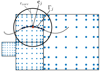
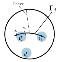
Fig. 5: (Left) A boundary segment ΓjsubscriptΓ𝑗\Gamma_{j} wth center point 𝐜jsubscript𝐜𝑗{\bf c}_{j} lying in a leaf node B𝐵B of side length rlsubscript𝑟𝑙r_{l}. Depending on the value of δ𝛿\delta, a boundary integral of the form (13) is either resolved by its discretization using standard Gauss-Legendre quadrature with k𝑘k nodes on ΓjsubscriptΓ𝑗\Gamma_{j}, or negligible outside the disk centered at 𝐜jsubscript𝐜𝑗{\bf c}_{j} with radius rcorrsubscript𝑟𝑐𝑜𝑟𝑟r_{corr}, which we will denote by Djsubscript𝐷𝑗D_{j}. (Right) In the latter case (when δ𝛿\delta is small and the Gaussian is sharply peaked), a simple interpolatory rule can be used to compute the correct contribution using O(k2)𝑂superscript𝑘2O(k^{2}) work per target point, either on or off the boundary. The shaded circles in the figure around the three target points 𝐭isubscript𝐭𝑖{\bf t}_{i} are meant to indicate the regions where the Gaussians centered at 𝐭isubscript𝐭𝑖{\bf t}_{i} are less than a user-prescribed tolerance ϵitalic-ϵ\epsilon. 𝐭1subscript𝐭1{\bf t}_{1} is sufficiently far from ΓjsubscriptΓ𝑗\Gamma_{j} that it can be ignored. 𝐭2subscript𝐭2{\bf t}_{2} and 𝐭3subscript𝐭3{\bf t}_{3} are off and on the boundary, respectively. The relevant portion of ΓjsubscriptΓ𝑗\Gamma_{j} for 𝐭2subscript𝐭2{\bf t}_{2} is marked in terms of the parameter s𝑠s by slsubscript𝑠𝑙s_{l} and srsubscript𝑠𝑟s_{r}.

Suppose now that we apply composite Gauss-Legendre quadrature to the integrals in (13). For the “single layer” type integral, we have

𝒮[σ](𝐱)=Γe|𝐱𝐲(s)|2δσ(𝐲(s))𝑑s𝐲j=1Mbi=0k1e|𝐱𝐲ij|2δσijwij,𝒮delimited-[]𝜎𝐱subscriptΓsuperscript𝑒superscript𝐱𝐲𝑠2𝛿𝜎𝐲𝑠differential-dsubscript𝑠𝐲superscriptsubscript𝑗1subscript𝑀𝑏superscriptsubscript𝑖0𝑘1superscript𝑒superscript𝐱subscript𝐲𝑖𝑗2𝛿subscript𝜎𝑖𝑗subscript𝑤𝑖𝑗{\cal S}[\sigma]({\bf x})=\int_{\Gamma}e^{-\frac{|{\bf x}-{\bf y}(s)|^{2}}{\delta}}\sigma({\bf y}(s))\,ds_{{\bf y}}\,\approx\sum_{j=1}^{M_{b}}\sum_{i=0}^{k-1}e^{-\frac{|{\bf x}-{\bf y}_{ij}|^{2}}{\delta}}\sigma_{ij}w_{ij}\,, (54)

where 𝐲ij=(yij1,yij2)subscript𝐲𝑖𝑗subscriptsuperscript𝑦1𝑖𝑗subscriptsuperscript𝑦2𝑖𝑗{\bf y}_{ij}=(y^{1}_{ij},y^{2}_{ij}) is the location of the i𝑖ith scaled Gauss-Legendre node on ΓjsubscriptΓ𝑗\Gamma_{j}, σijsubscript𝜎𝑖𝑗\sigma_{ij} is the density value at that point, and wij=wi[dyj1/ds(si)]2+[dyj2/ds(si)]2subscript𝑤𝑖𝑗subscript𝑤𝑖superscriptdelimited-[]𝑑subscriptsuperscript𝑦1𝑗𝑑𝑠subscript𝑠𝑖2superscriptdelimited-[]𝑑subscriptsuperscript𝑦2𝑗𝑑𝑠subscript𝑠𝑖2w_{ij}=w_{i}\sqrt{[dy^{1}_{j}/ds(s_{i})]^{2}+[dy^{2}_{j}/ds(s_{i})]^{2}}. Here, sisubscript𝑠𝑖s_{i} and wisubscript𝑤𝑖w_{i} denote the standard Gauss-Legendre nodes and weights on [1,1]11[-1,1].

Note that the quadrature weight wijsubscript𝑤𝑖𝑗w_{ij} involves both the standard weight wisubscript𝑤𝑖w_{i} and the change of variables corresponding to an arc-length parametrization on each segment. The necessary derivatives can be computed from (53). Note also that the sum in (54) consists simply of point sources and is easily incorporated into the FGT above. The only remaining issue has to do with the accuracy of the formula (54), since the smoothness of the integrand depends strongly on the parameter δ𝛿\delta. Here, however, the rapid decay of the Gaussian makes the problem tractable for any δ𝛿\delta. To see why, consider a boundary segment ΓjsubscriptΓ𝑗\Gamma_{j}, centered at 𝐜jsubscript𝐜𝑗{\bf c}_{j} in a leaf box B𝐵B of commensurate size (Fig. 5, left). Suppose first that δ𝛿\delta is sufficiently large that |Γj|C(ϵ)δsubscriptΓ𝑗𝐶italic-ϵ𝛿|\Gamma_{j}|\leq C(\epsilon)\sqrt{\delta}. C(ϵ)𝐶italic-ϵC(\epsilon) is straightforward to tabulate in terms of the user-specified tolerance ϵitalic-ϵ\epsilon. Then, it is straightforward to show that the error in k𝑘k-point Gauss-Legendre quadrature is of the order

EkC(e|Γj|216δk)ksubscript𝐸𝑘superscript𝐶superscript𝑒superscriptsubscriptΓ𝑗216𝛿𝑘𝑘E_{k}\approx C^{\prime}\left(\frac{e|\Gamma_{j}|^{2}}{16\delta k}\right)^{k}

for some constant Csuperscript𝐶C^{\prime}. This follows from the error estimate for Gauss-Legendre quadrature [9],

E(ba)2k+1(k!)4(2k+1)[(2k)!]3f(2k)𝐸superscript𝑏𝑎2𝑘1superscript𝑘42𝑘1superscriptdelimited-[]2𝑘3subscriptnormsuperscript𝑓2𝑘E\leq\frac{(b-a)^{2k+1}(k!)^{4}}{(2k+1)[(2k)!]^{3}}\|f^{(2k)}\|_{\infty}

for the integral abf(x)𝑑xsuperscriptsubscript𝑎𝑏𝑓𝑥differential-d𝑥\int_{a}^{b}f(x)\,dx, Stirling’s formula, and Cramer’s inequality. In short, the k𝑘k-point quadrature rule is spectrally accurate. Suppose now that |Γj|>C(ϵ)δsubscriptΓ𝑗𝐶italic-ϵ𝛿|\Gamma_{j}|>C(\epsilon)\sqrt{\delta}, and let rcorr=|Γj|subscript𝑟𝑐𝑜𝑟𝑟subscriptΓ𝑗r_{corr}=|\Gamma_{j}|. Then, for any target outside the circle of radius rcorrsubscript𝑟𝑐𝑜𝑟𝑟r_{corr} centered at 𝐜jsubscript𝐜𝑗{\bf c}_{j}, the integrand is bounded by eC(ϵ)2/4|Γj|σsuperscript𝑒𝐶superscriptitalic-ϵ24subscriptΓ𝑗subscriptnorm𝜎e^{-C(\epsilon)^{2}/4}\,|\Gamma_{j}|\,\|\sigma\|_{\infty}. (Setting C=12𝐶12C=12, the integrand is approximately |Γj|σ(21016)subscriptΓ𝑗subscriptnorm𝜎2superscript1016|\Gamma_{j}|\,\|\sigma\|_{\infty}\,(2\,\cdot 10^{-16}).) Thus, for each boundary segment with |Γj|>C(ϵ)δsubscriptΓ𝑗𝐶italic-ϵ𝛿|\Gamma_{j}|>C(\epsilon)\sqrt{\delta}, it remains only to correct the result obtained from the FGT within this circle Djsubscript𝐷𝑗D_{j} (Fig. 5, right).

This correction can be computed rapidly and accurately as follows. Let us denote by D(𝐭,r)𝐷𝐭𝑟D({\bf t},r) the circle of radius r𝑟r centered at 𝐭𝐭{\bf t} for any target 𝐭𝐭{\bf t} in the circle, where r=δln(1/ϵ)𝑟𝛿1italic-ϵr=\sqrt{\delta\ln(1/\epsilon)} so that e𝐭𝐲2/δ<ϵsuperscript𝑒superscriptnorm𝐭𝐲2𝛿italic-ϵe^{-\|{\bf t}-{\bf y}\|^{2}/\delta}<\epsilon. If D(𝐭,r)𝐷𝐭𝑟D({\bf t},r) doesn’t intersect ΓjsubscriptΓ𝑗\Gamma_{j}, the field is negligible and no correction is needed. Otherwise, we compute the intersection of ΓjsubscriptΓ𝑗\Gamma_{j} and D(𝐭,r)𝐷𝐭𝑟D({\bf t},r) and let the endpoints of the intersection be denoted by slsubscript𝑠𝑙s_{l} and srsubscript𝑠𝑟s_{r} (in terms of the underlying parametrization of ΓjsubscriptΓ𝑗\Gamma_{j}). We then interpolate the source distribution σ(s)𝜎𝑠\sigma(s) to kcsubscript𝑘𝑐k_{c} scaled Gauss-Legendre nodes on ΓjssuperscriptsubscriptΓ𝑗𝑠\Gamma_{j}^{s} for s[sl,sr]𝑠subscript𝑠𝑙subscript𝑠𝑟s\in[s_{l},s_{r}], and replace the original k𝑘k-point quadrature on ΓjsubscriptΓ𝑗\Gamma_{j} by a kcsubscript𝑘𝑐k_{c}-point Gauss-Legendre rule on [sl,sr]subscript𝑠𝑙subscript𝑠𝑟[s_{l},s_{r}]. Setting kcsubscript𝑘𝑐k_{c} to 20 yields approximately fourteen digits of accuracy assuming the density σ(s)𝜎𝑠\sigma(s) is locally smooth.

4.3 Periodic boundary conditions

It is straightforward to extend the FGT to handle periodic conditions on the unit square D=[0.5,0.5]2𝐷superscript0.50.52D=[-0.5,0.5]^{2}. Conceptually speaking, this can be accomplished by tiling the entire plane 𝐑2superscript𝐑2{\bf R}^{2} with copies of the source distribution f𝑓f. For this, we let Λ={𝐣=(j1,j2)|j1,j2𝐙}Λconditional-set𝐣subscript𝑗1subscript𝑗2subscript𝑗1subscript𝑗2𝐙\Lambda=\{{\bf j}=(j_{1},j_{2})|j_{1},j_{2}\in{\bf Z}\}. The tile T𝐣subscriptT𝐣{\rm T}_{{\bf j}} is a unit square centered at the lattice point 𝐣Λ𝐣Λ{\bf j}\in\Lambda. The extended periodic source distribution will be denoted by f~~𝑓\tilde{f}. From this, the solution to the periodic problem can be written as:

F~(𝐱)=𝐑2e|𝐱𝐲|2δf~(𝐲)𝑑𝐲.𝐱D.formulae-sequence~𝐹𝐱subscriptsuperscript𝐑2superscript𝑒superscript𝐱𝐲2𝛿~𝑓𝐲differential-d𝐲𝐱𝐷\tilde{F}({\bf x})=\int_{{\bf R}^{2}}e^{-\frac{|{\bf x}-{\bf y}|^{2}}{\delta}}\tilde{f}({\bf y})\,d{\bf y}.\;\;\;{\bf x}\in D.

As in the FMM for the Poisson equation [13, 11], we can accomodate periodic boundary conditions with very little change to the data structure or processing. To see this, note that, if we carry out the upward pass of the FGT until the root node (level l=0𝑙0l=0), we obtain an Hermite expansion describing the field due to all sources in D𝐷D. Because of the translation invariance of the kernel, the coefficients of this expansion are the same for every tile T𝐣subscriptT𝐣{\rm T}_{{\bf j}} covering the plane, expanded about the corresponding lattice point 𝐣𝐣{\bf j}. We denote the expansion about 𝐣𝐣{\bf j} by

ϕ(𝐱)=αpAαhα(𝐱𝐣δ).italic-ϕ𝐱subscript𝛼𝑝subscript𝐴𝛼subscript𝛼𝐱𝐣𝛿\phi({\bf x})=\sum_{\alpha\leq p}A_{\alpha}h_{\alpha}\left(\frac{{\bf x}-{\bf j}}{\sqrt{\delta}}\right).

Let us now define the punctured lattice by

Λ=Λ{(1,1),(1,0),(1,1),(0,1),(0,1),(1,1),(1,0),(1,1)}.superscriptΛΛ1110110101111011\Lambda^{\prime}=\Lambda-\{(-1,-1),(-1,0),(-1,1),(0,-1),(0,1),(1,-1),(1,0),(1,1)\}.

Having deleted the colleagues of the original unit box D𝐷D, centered at the origin, the remaining tiles indexed by ΛsuperscriptΛ\Lambda^{\prime} are all well separated from D𝐷D. From Lemma 6 and the linearity of the problem, it is clear that the contribution to field in D𝐷D from all well-separated tiles indexed by ΛsuperscriptΛ\Lambda^{\prime} can be representation by a local expansion

F~far(𝐱)=β0Cβ(𝐱δ)β,subscript~𝐹𝑓𝑎𝑟𝐱subscript𝛽0subscript𝐶𝛽superscript𝐱𝛿𝛽\tilde{F}_{far}({\bf x})=\sum_{\beta\geq 0}C_{\beta}\left(\frac{{\bf x}}{\sqrt{\delta}}\right)^{\beta}, (55)

centered at the origin, with coefficients

Cβ=(1)|β|β!αpAαα+βsubscript𝐶𝛽superscript1𝛽𝛽subscript𝛼𝑝subscript𝐴𝛼subscript𝛼𝛽C_{\beta}=\frac{(-1)^{|\beta|}}{\beta!}\sum_{\alpha\leq p}A_{\alpha}{\cal L}_{\alpha+\beta} (56)

where

α+β=𝐣Λhα+β(𝐣δ).subscript𝛼𝛽subscript𝐣superscriptΛsubscript𝛼𝛽𝐣𝛿{\cal L}_{\alpha+\beta}=\sum_{{\bf j}\in\Lambda^{\prime}}h_{\alpha+\beta}\left(\frac{{\bf j}}{\sqrt{\delta}}\right). (57)

Extending Definitions 10-12, we let Ψ0,1subscriptΨ01\Psi_{0,1} denote the local expansion for the root node D𝐷D at level 00, and define the nine tiles centered at ΛΛΛsuperscriptΛ\Lambda-\Lambda^{\prime} to be the root node’s colleagues.

When δ𝛿\delta is so small that lcut0subscript𝑙𝑐𝑢𝑡0l_{cut}\geq 0, the far field F~far(𝐱)subscript~𝐹𝑓𝑎𝑟𝐱\tilde{F}_{far}({\bf x}) in the root node D𝐷D is negligible (for given accuracy ϵitalic-ϵ\epsilon), so that we can initialize its coefficients Cβ=0subscript𝐶𝛽0C_{\beta}=0. Otherwise, we carry out the computation in (56) to initialize Ψ1,0subscriptΨ10\Psi_{1,0}. This requires the computation of tte lattice sums in (57). These are obtained rapidly from the Poisson summation formula:

j1=j2=hα((j1,j2)δ)=π2δ2(2πiδ)α1+α2(m=mα1eπ2m2δ)(n=nα2eπ2n2δ).superscriptsubscriptsubscript𝑗1superscriptsubscriptsubscript𝑗2subscript𝛼subscript𝑗1subscript𝑗2𝛿superscript𝜋2superscript𝛿2superscript2𝜋𝑖𝛿subscript𝛼1subscript𝛼2superscriptsubscript𝑚superscript𝑚subscript𝛼1superscript𝑒superscript𝜋2superscript𝑚2𝛿superscriptsubscript𝑛superscript𝑛subscript𝛼2superscript𝑒superscript𝜋2superscript𝑛2𝛿\begin{split}\sum_{j_{1}=-\infty}^{\infty}\sum_{j_{2}=-\infty}^{\infty}&h_{\alpha}\left(\frac{(j_{1},j_{2})}{\sqrt{\delta}}\right)=\\ &\pi^{2}\delta^{2}(-2\pi i\sqrt{\delta})^{\alpha_{1}+\alpha_{2}}\left(\sum_{m=-\infty}^{\infty}m^{\alpha_{1}}\cdot e^{-\pi^{2}m^{2}\delta}\right)\left(\sum_{n=-\infty}^{\infty}n^{\alpha_{2}}\cdot e^{-\pi^{2}n^{2}\delta}\right).\end{split} (58)

It is straightforward to verify that, when δ𝛿\delta is large enough that F~far(𝐱)subscript~𝐹𝑓𝑎𝑟𝐱\tilde{F}_{far}({\bf x}) is non-negligible, only a few terms are required on the right-hand side of (58) and only milliseconds are needed for all α+βsubscript𝛼𝛽{\cal L}_{\alpha+\beta}.

Only two other changes are needed in the FGT: the interaction list and near neighbor computations must be adjusted to account for periodic images. Having defined the colleagues of the root node above, this is handled automatically by the data structure. For large scale problems with many levels of refinement, this involves a modest increase in work for boxes near the boudary of D𝐷D and a negligible increase in the total work.

5 Numerical results

In this section, we illustrate the performance of both the volume and boundary FGT, implemented in Fortran, with experiments carried out on a single core of a 3.4GHz Intel Xeon processor. Our first example demonstrates the linear scaling of CPU time with the number of grid points. We compute the volume FGT

Gδ[fk](𝐱)=𝐑2e|𝐱𝐲|2δf(𝐲)𝑑𝐲,subscript𝐺𝛿delimited-[]subscript𝑓𝑘𝐱subscriptsuperscript𝐑2superscript𝑒superscript𝐱𝐲2𝛿𝑓𝐲differential-d𝐲G_{\delta}[f_{k}]({\bf x})=\int_{{\bf R}^{2}}e^{-\frac{|{\bf x}-{\bf y}|^{2}}{\delta}}f({\bf y})d{\bf y}\,, (59)

with the source distribution

fk(𝐱)=sin(2kπx1)cos(2kπx2)(k𝐙),subscript𝑓𝑘𝐱2𝑘𝜋subscript𝑥12𝑘𝜋subscript𝑥2𝑘𝐙f_{k}({\bf x})=\sin(2k\pi x_{1})\cos(2k\pi x_{2})\;\;\;(k\in{\bf Z}), (60)

imposing periodic boundary conditions.

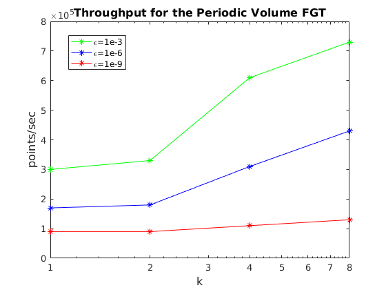
In order for the numerical experiment to be non-trivial, we increase the complexity of the problem as we increase the number of degrees of freedom. More precisely, we consider four cases, with k=1,2,4,8𝑘1248k=1,2,4,8 and δ=1k2𝛿1superscript𝑘2\delta=\frac{1}{k^{2}}, requiring a finer and finer spatial mesh to resolve the data. For each choice of k𝑘k, we create a (level-restricted) quadtree, refined to a level where fksubscript𝑓𝑘f_{k} is accurately represented with our piecewise eighth order polynomial to 10 digits of accuracy. For the function described in (60), the refinement happens to be uniform, with N=256,1024,4096,16384𝑁2561024409616384N=256,1024,4096,16384 leaf nodes for the four cases, respectively. (We will see examples with inhomgeneous source distributions and adaptive data structures below.) Timings are given in Table 1 and plotted in Fig. 6.
k𝑘k
ϵitalic-ϵ\epsilon 111 222 444 888
103superscript10310^{-3} 3.01053.0superscript1053.0\cdot 10^{5} 3.31053.3superscript1053.3\cdot 10^{5} 6.11056.1superscript1056.1\cdot 10^{5} 7.31057.3superscript1057.3\cdot 10^{5}
106superscript10610^{-6} 1.71051.7superscript1051.7\cdot 10^{5} 1.81051.8superscript1051.8\cdot 10^{5} 3.11053.1superscript1053.1\cdot 10^{5} 4.31054.3superscript1054.3\cdot 10^{5}
109superscript10910^{-9} 0.91050.9superscript1050.9\cdot 10^{5} 0.91050.9superscript1050.9\cdot 10^{5} 1.11051.1superscript1051.1\cdot 10^{5} 1.31051.3superscript1051.3\cdot 10^{5}
Table 1: Throughput on a single core for the volume FGT with periodic boundary condition in units of points/second.
Refer to caption
Fig. 6: Throughput for the volume FGT (measured in units of 100,000100000100,000 points/second) with various precisions, plotted as a function of δ𝛿\delta. (The data is the same as in Table 1.)

While the cost appears to grow in a sublinear fashion with the number of grid points, this is simply because of the non-trivial cost of the precomputation. A more precise model for the CPU time takes the form

T(N,ϵ)=A(ϵ)N+B(ϵ)logN𝑇𝑁italic-ϵ𝐴italic-ϵ𝑁𝐵italic-ϵ𝑁T(N,\epsilon)=A(\epsilon)N+B(\epsilon)\log N (61)

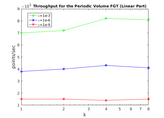
for precision ϵitalic-ϵ\epsilon. The term B(ϵ)logN𝐵italic-ϵ𝑁B(\epsilon)\log N is dominated by the building of tables for the local interactions, which is done once per level. In the present example, the sublinear part contributes about 30 % of the cost for the smaller problem sizes and less than 10 % for the largest N𝑁N. If we subtract the time for precomputation/table building, and measure the time of the remainder of the FGT, we see a steady “throughput,” measured in points per second for each fixed precision. This verifies the linear scaling (Table 2 and Fig. 7).
k𝑘k
ϵitalic-ϵ\epsilon 111 222 444 888
103superscript10310^{-3} 7.01057.0superscript1057.0\cdot 10^{5} 7.21057.2superscript1057.2\cdot 10^{5} 8.21058.2superscript1058.2\cdot 10^{5} 8.11058.1superscript1058.1\cdot 10^{5}
106superscript10610^{-6} 3.81053.8superscript1053.8\cdot 10^{5} 4.01054.0superscript1054.0\cdot 10^{5} 4.31054.3superscript1054.3\cdot 10^{5} 4.11054.1superscript1054.1\cdot 10^{5}
109superscript10910^{-9} 1.51051.5superscript1051.5\cdot 10^{5} 1.51051.5superscript1051.5\cdot 10^{5} 1.41051.4superscript1051.4\cdot 10^{5} 1.51051.5superscript1051.5\cdot 10^{5}
Table 2: Throughput on a single core for the volume FGT with periodic boundary condition in units of points/second.
Refer to caption
Fig. 7: Throughput for the volume FGT (measured in units of 100,000100000100,000 points/second) with various precisions, plotted as a function of δ𝛿\delta. (The data is the same as in Table 2.)

For our second example, we again compute the volume FGT with periodic boundary condition where fksubscript𝑓𝑘f_{k} is given by (60) with k=2𝑘2k=2. Gδ[fk]subscript𝐺𝛿delimited-[]subscript𝑓𝑘G_{\delta}[f_{k}] is available analytically for this fk(𝐱)subscript𝑓𝑘𝐱f_{k}({\bf x}) from Fourier analysis. The source distribution is again resolved to 10 digits of accuracy, but we now compute the FGT with requested precisions of ϵ=103italic-ϵsuperscript103\epsilon=10^{-3}, 106superscript10610^{-6} and 109superscript10910^{-9}. For each choice of ϵitalic-ϵ\epsilon, we carry out the computation for a wide range of δ𝛿\delta, from δ=107𝛿superscript107\delta=10^{-7} to δ=101𝛿superscript101\delta=10^{-1}. Timings are provided in Table 3 and plotted in Fig. 8.
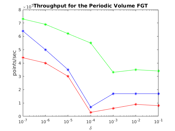
δ𝛿\delta
ϵitalic-ϵ\epsilon 101superscript10110^{-1} 102superscript10210^{-2} 103superscript10310^{-3} 104superscript10410^{-4} 105superscript10510^{-5} 106superscript10610^{-6} 107superscript10710^{-7}
103superscript10310^{-3} 3.41053.4superscript1053.4\cdot 10^{5} 3.51053.5superscript1053.5\cdot 10^{5} 3.31053.3superscript1053.3\cdot 10^{5} 5.51055.5superscript1055.5\cdot 10^{5} 6.21056.2superscript1056.2\cdot 10^{5} 6.91056.9superscript1056.9\cdot 10^{5} 7.31057.3superscript1057.3\cdot 10^{5}
106superscript10610^{-6} 1.71051.7superscript1051.7\cdot 10^{5} 1.71051.7superscript1051.7\cdot 10^{5} 1.71051.7superscript1051.7\cdot 10^{5} 0.71050.7superscript1050.7\cdot 10^{5} 3.01053.0superscript1053.0\cdot 10^{5} 5.01055.0superscript1055.0\cdot 10^{5} 5.41055.4superscript1055.4\cdot 10^{5}
109superscript10910^{-9} 0.81050.8superscript1050.8\cdot 10^{5} 0.91050.9superscript1050.9\cdot 10^{5} 0.61050.6superscript1050.6\cdot 10^{5} 0.31050.3superscript1050.3\cdot 10^{5} 3.51053.5superscript1053.5\cdot 10^{5} 4.01054.0superscript1054.0\cdot 10^{5} 4.41054.4superscript1054.4\cdot 10^{5}
Table 3: Throughput on a single core for the volume FGT with periodic boundary condition in units of points/second.
Refer to caption
Fig. 8: Throughput for the volume FGT (measured in units of 100,000100000100,000 points/second) with various precisions, plotted as a function of δ𝛿\delta. (The data is the same as in Table 3.)

Our third example illustrates the performance of the FGT with an adaptive data structure. For this, we let B𝐵B denote the unit box with f𝑓f given by

f(𝐱)=i=15eαi|𝐱𝐱i|2,𝑓𝐱superscriptsubscript𝑖15superscript𝑒subscript𝛼𝑖superscript𝐱subscript𝐱𝑖2f({\bf x})=\sum_{i=1}^{5}e^{-\alpha_{i}|{\bf x}-{\bf x}_{i}|^{2}}\,, (62)

with

[𝐱1,,𝐱5]=[(0.20,0.10),(0.31,0.50),(0.68,0.40),(0.41,0.80),(0.12,0.45)]subscript𝐱1subscript𝐱50.200.100.310.500.680.400.410.800.120.45[{\bf x}_{1},\dots,{\bf x}_{5}]=[(0.20,0.10),(0.31,0.50),(0.68,0.40),(0.41,0.80),(0.12,0.45)]

and

[α1,,α5]=(0.010,0.005,0.003,0.002,0.001).subscript𝛼1subscript𝛼50.0100.0050.0030.0020.001[\alpha_{1},\dots,\alpha_{5}]=(0.010,0.005,0.003,0.002,0.001).
Refer to caption
Refer to caption
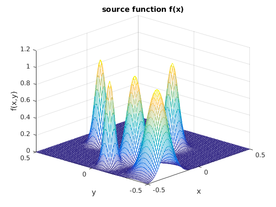
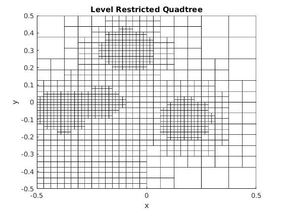
Fig. 9: (Left) Plot of the volume source distribution, which is taken to be the sum of a few Gaussians. (Right) A level restricted quadtree on which the source distribution is resolved to 10 digits of accuracy as a piecewise polynomial of degree 8.

Gδ[f]subscript𝐺𝛿delimited-[]𝑓G_{\delta}[f] is available analytically for this choice of f(𝐱)𝑓𝐱f({\bf x}). In Fig. 9, we plot the source distribution along with a level restricted quadtree on which the source distribution is resolved to ten digits of accuracy. We compute the volume FGT with requested precisions of ϵ=103italic-ϵsuperscript103\epsilon=10^{-3}, 106superscript10610^{-6} and 109superscript10910^{-9}. For each choice of ϵitalic-ϵ\epsilon, we carry out the computation for a wide range of δ𝛿\delta, from δ=107𝛿superscript107\delta=10^{-7} to δ=101𝛿superscript101\delta=10^{-1}. Timings are given in Table 4 and plotted in Fig. 10.
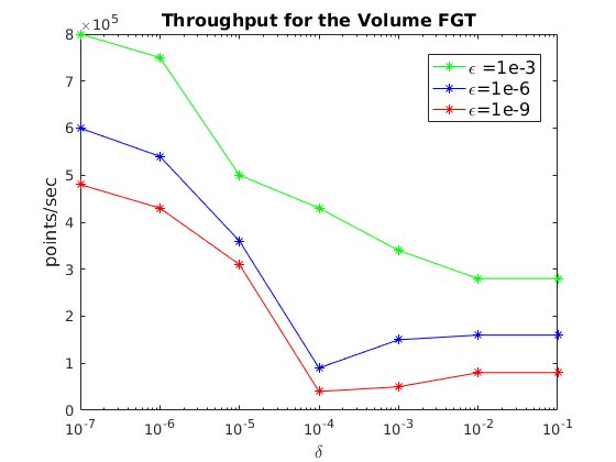
δ𝛿\delta
ϵitalic-ϵ\epsilon 101superscript10110^{-1} 102superscript10210^{-2} 103superscript10310^{-3} 104superscript10410^{-4} 105superscript10510^{-5} 106superscript10610^{-6} 107superscript10710^{-7}
103superscript10310^{-3} 2.81052.8superscript1052.8\cdot 10^{5} 2.81052.8superscript1052.8\cdot 10^{5} 3.41053.4superscript1053.4\cdot 10^{5} 4.31054.3superscript1054.3\cdot 10^{5} 5.01055.0superscript1055.0\cdot 10^{5} 7.51057.5superscript1057.5\cdot 10^{5} 8.01058.0superscript1058.0\cdot 10^{5}
106superscript10610^{-6} 1.61051.6superscript1051.6\cdot 10^{5} 1.61051.6superscript1051.6\cdot 10^{5} 1.51051.5superscript1051.5\cdot 10^{5} 0.91050.9superscript1050.9\cdot 10^{5} 3.11053.1superscript1053.1\cdot 10^{5} 5.41055.4superscript1055.4\cdot 10^{5} 6.01056.0superscript1056.0\cdot 10^{5}
109superscript10910^{-9} 0.81050.8superscript1050.8\cdot 10^{5} 0.81050.8superscript1050.8\cdot 10^{5} 0.51050.5superscript1050.5\cdot 10^{5} 0.41050.4superscript1050.4\cdot 10^{5} 3.61053.6superscript1053.6\cdot 10^{5} 4.31054.3superscript1054.3\cdot 10^{5} 4.81054.8superscript1054.8\cdot 10^{5}
Table 4: Throughput on a single core for the volume FGT in units of points/second. This is a useful benchmark for linear scaling algorithms, permitting simple estimation of the performance in terms of CPU time to any problem size.
Refer to caption
Fig. 10: Throughput for the volume FGT (measured in units of 100,000100000100,000 points/second) with various precisions, plotted as a function of δ𝛿\delta. (The data is the same as in Table 4.)

Note that, for a fixed tolerance ϵitalic-ϵ\epsilon, the performance of the volume FGT is relatively insensitive to the parameter δ𝛿\delta. For large δ𝛿\delta, the far field is nontrivial but very smooth. For sufficiently small δ𝛿\delta, the interaction is entirely local and the FGT is particularly fast. The worst case performance is for δ104𝛿superscript104\delta\approx 10^{-4}, where both the far field and near field need significant effort.

Our fourth example illustrates the performance of the boundary FGT. We compute the integral

Gδ[f](𝐱)=Γe|𝐱𝐲|2δf(𝐲)𝑑𝐲,subscript𝐺𝛿delimited-[]𝑓𝐱subscriptΓsuperscript𝑒superscript𝐱𝐲2𝛿𝑓𝐲differential-d𝐲G_{\delta}[f]({\bf x})=\int_{\Gamma}e^{-\frac{|{\bf x}-{\bf y}|^{2}}{\delta}}f({\bf y})d{\bf y}\,, (63)

where ΓΓ\Gamma is chosen to be the ellipse:

{y1(θ)=0.45cos(θ),y2(θ)=0.25sin(θ),(0θ2π).casessubscript𝑦1𝜃0.45𝜃otherwisesubscript𝑦2𝜃0.25𝜃otherwise0𝜃2𝜋\begin{cases}y_{1}(\theta)=0.45\cos(\theta),\\ y_{2}(\theta)=0.25\sin(\theta),\end{cases}(0\leq\theta\leq 2\pi)\,. (64)

We let

f(𝐱)=cos(2x1)+sin(x2),(𝐱Γ).𝑓𝐱2subscript𝑥1subscript𝑥2𝐱Γf({\bf x})=\cos(2x_{1})+\sin(x_{2}),\;\;\;({\bf x}\in\Gamma). (65)

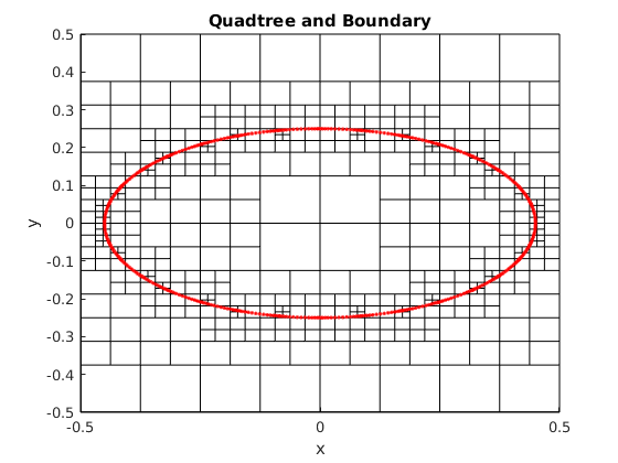
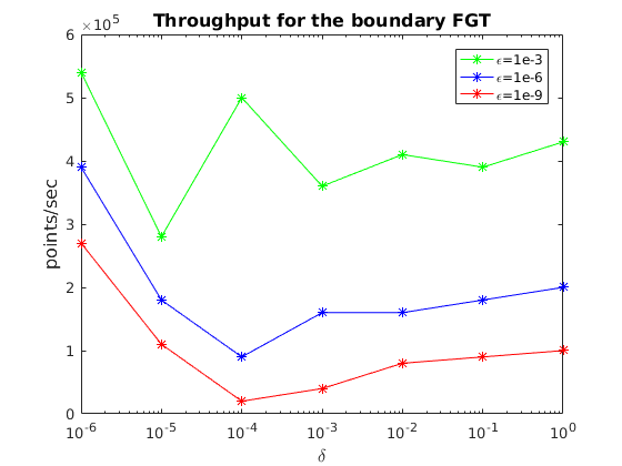
We create an adaptive quadtree on the unit box so that each leaf box of the tree contains no more than O(1)𝑂1O(1) boundary points and then enforce the level-restricted condition, yielding the data structure shown in Fig. 11. The leaf nodes with 888 tensor product Chebyshev grids on each define our volumetric targets. The boundary FGT is then evaluated at all volumetric grid points and all boundary points as well. Timings are given in Table 5 and plotted in Fig. 12.
Refer to caption
Fig. 11: A level-restricted quad tree determined by the discretization of the indicated ellipse.
δ𝛿\delta
ϵitalic-ϵ\epsilon 100superscript10010^{0} 101superscript10110^{-1} 102superscript10210^{-2} 103superscript10310^{-3} 104superscript10410^{-4} 105superscript10510^{-5} 106superscript10610^{-6}
103superscript10310^{-3} 4.21054.2superscript1054.2\cdot 10^{5} 3.91053.9superscript1053.9\cdot 10^{5} 4.11054.1superscript1054.1\cdot 10^{5} 3.61053.6superscript1053.6\cdot 10^{5} 5.01055.0superscript1055.0\cdot 10^{5} 2.81052.8superscript1052.8\cdot 10^{5} 5.41055.4superscript1055.4\cdot 10^{5}
106superscript10610^{-6} 2.01052.0superscript1052.0\cdot 10^{5} 1.81051.8superscript1051.8\cdot 10^{5} 1.61051.6superscript1051.6\cdot 10^{5} 1.61051.6superscript1051.6\cdot 10^{5} 0.91050.9superscript1050.9\cdot 10^{5} 1.81051.8superscript1051.8\cdot 10^{5} 3.91053.9superscript1053.9\cdot 10^{5}
109superscript10910^{-9} 1.01051.0superscript1051.0\cdot 10^{5} 0.91050.9superscript1050.9\cdot 10^{5} 0.81050.8superscript1050.8\cdot 10^{5} 0.41050.4superscript1050.4\cdot 10^{5} 0.21050.2superscript1050.2\cdot 10^{5} 1.11051.1superscript1051.1\cdot 10^{5} 2.71052.7superscript1052.7\cdot 10^{5}
Table 5: Throughput for the boundary FGT with volumetric targets, measured in points/second, for various precisions and values of δ𝛿\delta.
Refer to caption
Fig. 12: Throughput for the boundary FGT with boundary and volume targets, measured in points/second, for various precisions, plotted as a function of δ𝛿\delta.

Note, again, that the performance of the boundary FGT varies only modestly over a wide range of the parameter δ𝛿\delta. For sufficiently small δ𝛿\delta, the interaction is entirely local and no expansions are formed. For sufficiently large δ𝛿\delta, a smooth quadrature rule is accurate enough to discretize the boundary integral, avoiding the need for local correction. The code is slowest for intermediate values of δ𝛿\delta, where both local and far field contributions are significant (while still satisfying linear scaling with the number of source and target points).

5.1 An initial value problem for the heat equation

As a final example, we consider the homogeneous heat equation:

ut(𝐱,t)=Δu(𝐱,t),u(𝐱,0)=f(𝐱)formulae-sequencesubscript𝑢𝑡𝐱𝑡Δ𝑢𝐱𝑡𝑢𝐱0𝑓𝐱\begin{split}u_{t}({\bf x},t)&=\Delta u({\bf x},t),\\ u({\bf x},0)&=f({\bf x})\end{split} (66)

for 𝐱D=[0.5,0.5]2𝐱𝐷superscript0.50.52{\bf x}\in D=[-0.5,0.5]^{2}, with periodic boundary conditions. The initial data is chosen to be a piecewise constant function:

f(𝐱)=Ci,for𝐱Di,formulae-sequence𝑓𝐱subscript𝐶𝑖for𝐱subscript𝐷𝑖f({\bf x})=C_{i},\;\;\;{\rm for}\;\;{\bf x}\in D_{i}, (67)

where the unit box D𝐷D is refined uniformly on a tree that is five levels deep, resulting in a 32-by-32 grid of leaf nodes Disubscript𝐷𝑖D_{i}. On each leaf node, we let Cisubscript𝐶𝑖C_{i} take on a random value in the range [0,1]01[0,1]. f(x)𝑓𝑥f(x) is plotted in Fig. 13.

The exact solution of this problem is given by:

u(𝐱,t)=14πt𝐑2e|𝐱𝐲|24tf~(𝐲)𝑑𝐲,𝑢𝐱𝑡14𝜋𝑡subscriptsuperscript𝐑2superscript𝑒superscript𝐱𝐲24𝑡~𝑓𝐲differential-d𝐲u({\bf x},t)=\frac{1}{4\pi t}\int_{{\bf R}^{2}}e^{-\frac{|{\bf x}-{\bf y}|^{2}}{4t}}\tilde{f}({\bf y})d{\bf y}, (68)

where f~~𝑓\tilde{f} is the periodic extension of f𝑓f. This is precisely what is computed by the periodic version of the volume FGT and the solution u(𝐱,t)𝑢𝐱𝑡u({\bf x},t) is plotted for various choices of t𝑡t in Fig. 13, with nine digits of precision in the FGT.

Remark 3.

There is a subtle issue regarding the use of the FGT to compute (68), namely that the error estimates for the FGT derived above are based on the Gaussian rather than the heat kernel, which includes the additional 1/(4πt)14𝜋𝑡1/(4\pi t) scaling in two dimensions. To compute an accurate convolution requires that the local tables be built using the full heat kernel (whose support to a fixed precision ϵitalic-ϵ\epsilon is slightly greater than the support of the Gaussian alone). The far field and local expansions also require a few more terms. Without entering into a detailed analysis, we illustrate the difference when t=104𝑡superscript104t=10^{-4} for leaf node boxes in the present example. For the FGT, Hermite expansions of order p=22𝑝22p=22 are needed to achieve 9 digits of precision. For the full heat kernel, it turns out that p=28𝑝28p=28 is required to achieve the same accuracy.
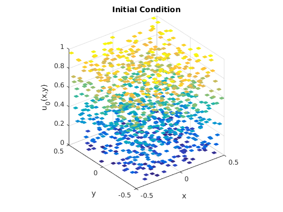
Refer to caption
Refer to caption
Refer to caption
Refer to caption
Fig. 13: The solution to the heat equation on a box with periodic boundary conditions and piecewise constant initial data, plotted at various times

6 Conclusions

We have presented a new adaptive version of the fast Gauss transform (FGT) which can be used for the evaluation of volume or boundary integrals with a Gaussian kernel as well as the field induced by discrete point sources. This is a standard and well-defined computational task in its own right, and serves as a key component in integral equation-based solvers for the heat equation in complex geometry [32]. The extension of the present method to three dimensions is straightforward and will be reported at a later date.

References

  • [1] D. N. Arnold and P. Noon, Coercivity of the single layer heat potential, J. Comput. Math., 7 (1989), pp. 100–104.
  • [2] T. Askham and A. J. Cerfon, An adaptive fast multipole accelerated poisson solver for complex geometries, J. Comput. Phys., 344 (2017), pp. 1–22.
  • [3] B. J. C. Baxter and G. Roussos, A new error estimate of the fast Gauss transform, SIAM Journal of Scientific Computing, 24 (2002), pp. 257–259.
  • [4] J. P. Boyd, Chebyshev and Fourier Spectral Methods, Dover, New York, 2001.
  • [5] R. M. Brown, The method of layer potentials for the heat equation in Lipschitz cylinders, Amer. J. Math., 111 (1989), pp. 339–379.
  • [6] H. Cheng, J. Huang, and T. J. Leiterman, An adaptive fast solver for the modified helmholtz equation in two dimensions, Journal of Computational Physics, 211 (2006), pp. 616–637.
  • [7] M. Costabel, Time-dependent problems with the boundary integral equation, in Encyclopedia of Computational Mechanics, E. Stein, R. de Borst, and T. J. R. Hughes, eds., John Wiley & Sons, 2004, pp. 703–721.
  • [8] G. F. Dargush and P. K. Banerjee, Application of the boundary element method to transient heat conduction, International Journal for Numerical Methods in Engineering, 31 (1991), pp. 1231–1247.
  • [9] P. J. Davis and P. Rabinowitz, Methods of numerical integration, Academic Press, San Diego, 1984.
  • [10] A. Elgammal, R. Duraiswami, and L. S. Davis, Efficient kernel density estimation using the fast Gauss transform with applications to color modeling and tracking, IEEE Transactions on Pattern Analysis and Machine Intelligence, 25 (2003), pp. 1499–1504.
  • [11] F. Ethridge and L. Greengard, A New Fast-Multipole Accelerated Poisson Solver in Two Dimensions, SIAM Journal on Scientific Computing, 23 (2001), pp. 741–760.
  • [12] L. Greengard and P. Lin, Spectral approximation of the free-space heat kernel, Appl. Comput. Harmon. Anal., 9 (2000), pp. 83–97.
  • [13] L. Greengard and V. Rokhlin, A fast algorithm for particle simulations, Journal of computational physics, 73 (1987), pp. 325–348.
  • [14] L. Greengard and J. Strain, The fast Gauss transform, SIAM J. Sci. Statist. Comput., 12 (1991), pp. 79–94.
  • [15] L. Greengard and X. Sun, A new version of the fast Gauss transform, Documenta Mathematica, III (1998), pp. 575–584.
  • [16] R. B. Guenther and J. W. Lee, Partial differential equations of mathematical physics and integral equations, Prentice Hall, Inglewood Cliffs, New Jersey, 1988.
  • [17] M. T. Ibanez and H. Power, An efficient direct bem numerical scheme for phase change problems using fourier series, Computer Methods in Applied Mechanics and Engineering, 191 (2002), pp. 2371–2402.
  • [18] H. Langston, L. Greengard, and D. Zorin, A free-space adaptive fmm-based pde solver in three dimensions, Comm. Appl. Math. and Comp. Sci., 6 (2011), pp. 79–122.
  • [19] D. Lee, A. Gray, and A. Moore, Dual-tree fast gauss transforms, Advances in Neural Information Processing Systems, 18 (2006), pp. 747–754.
  • [20] J.-Y. Lee and L. Greengard, A direct adaptive Poisson solver of arbitrary order accuracy, Journal of computational physics, 125 (1996), pp. 415–424.
  • [21] J.-R. Li and L. Greengard, High order accurate methods for the evaluation of layer heat potentials, SIAM J. Sci. Comput., 31 (2009), pp. 3847–3860.
  • [22] D. Malhotra and G. Biros, Algorithm 967: A distributed-memory fast multipole method for volume potentials, ACM Trans. Math. Softw., 43 (2016), pp. 17:1–17:27.
  • [23] W. Pogorzelski, Integral equations and their applications, Pergamon Press, Oxford, 1966.
  • [24] R. S. Sampath, H. Sundar, and S. Veerapaneni, Parallel fast gauss transform, in SC ’10: Proceedings of the ACM/IEEE International Conference for High Performance Computing, Networking, Storage and Analysis, New Orleans, LA, 2010, pp. 1–10.
  • [25] M. Spivak, S. Veerapaneni, and L. Greengard, The fast generalized gauss transform, SIAM J. Sci. Comput., 32 (2010), pp. 3092–3107.
  • [26] J. Strain, The fast gauss transform with variable scales, SIAM J. Sci. Stat. Comput., 12 (1991), pp. 1131–1139.
  • [27]  , Fast adaptive methods for the free-space heat equation, SIAM J. Sci. Comput., 15 (1994), pp. 185–206.
  • [28] J. Tausch and A. Weckiewicz, Multidimensional fast Gauss transforms by Chebyshev expansions, SIAM J. Sci. Comput., 31 (2009), pp. 3547–3565.
  • [29] S. K. Veerapaneni and G. Biros, A high-order solver for the heat equation in 1d domains with moving boundaries, SIAM J. Sci. Comput., 29 (2007), pp. 2581–2606.
  • [30]  , The Chebyshev fast Gauss and nonuniform fast Fourier transforms and their application to the evaluation of distributed heat potentials, J. Comput. Phys., 227 (2008), pp. 7768–7790.
  • [31] X. Wan and G. Karniadakis, A sharp error estimate for the fast Gauss transform, Journal of Computational Physics, 219 (2006), pp. 7–12.
  • [32] J. Wang, L. Greengard, S. Jiang, and S. K. Veerapaneni, A high-order solver for the two-dimensional heat equation in moving domains, in preparation, (2017).