Bayesian Analysis of the break in DAMPE Lepton Spectra

Abstract

Recently, DAMPE has released its first results on the high-energy cosmic-ray electrons and positrons (CREs) from about $25\,\mathrm{GeV}$ to $4.6\,\mathrm{TeV}$, which directly detect a break at $\sim 1\,\mathrm{TeV}$. This result gives us an excellent opportunity to study the source of the CREs excess. In this work, we used the data for proton and helium flux (from AMS-02 and CREAM), $\,\bar{\text{p}}/\text{p}$ ratio (from AMS-02), positron flux (from AMS-02) and CREs flux (from DAMPE without the peak signal point at $\sim 1.4\,\mathrm{TeV}$) to do global fitting simultaneously, which can account the influence from the propagation model, the nuclei and electron primary source injection and the secondary lepton production precisely. For extra source to interpret the excess in lepton spectrum, we consider two separate scenarios (pulsar and dark matter annihilation via leptonic channels) to construct the bump ($\gtrsim 100\,\mathrm{GeV}$) and the break at $\sim 1\,\mathrm{TeV}$. The result shows: (i) in pulsar scenario, the spectral index of the injection should be $\nu_{psr}\sim 0.65$ and the cut-off should be $R_{c}\sim 650\,\mathrm{GV}$; (ii) in dark matter scenario, the dark matter particle’s mass is $m_{\chi}\sim 1208\,\mathrm{GeV}$ and the cross section is $\langle\sigma v\rangle\sim 1.48\times 10^{-23}\,\mathrm{cm}^{3}\,\mathrm{s}^{-1}$. Moreover, in the dark matter scenario, the $\tau\bar{\tau}$ annihilation channel is highly suppressed, and a DM model is built to satisfy the fitting results.

I Introduction

Recently, DAMPE (DArk Matter Particle Explorer) (Chang, 2014; Chang et al., 2017) Satellite, which has been launched on December 17, 2015, has released its first data on high-energy cosmic-ray electrons and positrons (CREs) (Ambrosi et al., 2017). DAMPE has measured the CREs (i.e., $e^{-}+e^{+}$) spectrum in the range of $25\,\mathrm{GeV}-4.6\,\mathrm{TeV}$ with unprecedented energy resolution (better than $1.2\%$ $\gtrsim 100\,\mathrm{GeV}$). The results shows a bumps at about $100\,\mathrm{GeV}-1\,\mathrm{TeV}$ which is consistent with previous results (Adriani et al., 2009; PAMELA collaboration et al., 2010; AMS collaboration et al., 2014a; Fermi-LAT collaboration et al., 2012; collaboration et al., 2017a, b). More interesting, a break at $\sim 1\,\mathrm{TeV}$ and a peak signal at $\sim 1.4\,\mathrm{TeV}$ have been detected. All of these features cannot be described by a single power law and provide us an opportunity to study the source of high-energy CREs.

The peak signal at $\sim 1.4\,\mathrm{TeV}$ has been studied by many works which employed nearby pulsars wind, supernova remnants (SNRs) and dark matter (DM) sub-structures (Malyshev et al., 2009; Kuhlen and Malyshev, 2009; Brun et al., 2009; Gendelev et al., 2010; Profumo, 2012; Panov, 2013; Fang et al., 2017; Yuan et al., 2017a; Athron et al., 2017; Fan et al., 2017; Duan et al., 2017; Gu and He, 2017; Liu and Liu, 2017; Cao et al., 2017; Profumo et al., 2017). At the same time, considering the statistical confidence level of this signal is about $3\sigma$ which needs more counts in future, we exclude the peak signal and do a global fitting on the left points in DAMPE CREs spectrum in this work. As a result, if we refer to the DAMPE CREs flux in this work, the peak point is excluded except special emphasis.

In cosmic ray (CR) theory, the CR electrons are expected to be accelerated during the acceleration of CR nuclei at the sources, e.g. SNRs. But the CR positrons are produced as secondary particles from CR nuclei interaction with the interstellar medium (ISM) (Adriani et al., 2009; AMS collaboration et al., 2013a; Barwick et al., 1997; AMS-01 collaboration, 2007). From the results of the flux of positrons and electrons (AMS collaboration et al., 2013b, 2014b, 2014c, 2014a), we can infer that there should be some extra sources producing electron-positron pairs. This can be interpreted both by the astrophysical sources’ injection (Shen, 1970; Zhang and Cheng, 2001; Yüksel et al., 2009; Hooper et al., 2009; Profumo, 2012; Blasi, 2009; Hu et al., 2009; Fujita et al., 2009) and DM annihilation or decay (Bergström et al., 2008; Barger et al., 2009; Cirelli et al., 2009; Zhang et al., 2009; Bergström et al., 2009; Yin et al., 2013; Dev et al., 2014).

As a result, the CREs data contains the primary electrons, the secondary electrons, the secondary positrons and the extra source of electron-positron pairs. If we want to study the properties of the extra source, we should deduct the primary electrons and secondary electrons/positrons first. The primary electrons are always assumed to have a power-law form injection and the secondary electrons/positrons are determined dominatingly by the CR proton and helium particles interact with ISM. Consequently, we should do global fitting to these data simultaneously which can avoid the bias of choosing the lepton background parameters..

Considering the situations of high-dimentional parameter space of propagation model and precise data sets, we employ a Markov Chain Monte Carlo (MCMC (Lewis and Bridle, 2002)) method (embeded by dragon) to do global fitting and sample the parameter space of all the related parameters to reproduce the CREs spectrum (Liu et al., 2010; Lin et al., 2015; Yuan et al., 2017b; Niu and Li, 2018).

Moreover, because of the significant difference in the slopes of proton and helium, of about $\sim 0.1$ (Panov et al., 2006; Ahn et al., 2010; PAMELA collaboration et al., 2011a; AMS collaboration et al., 2015a, b), has been observed, we use separate primary source spectra settings for proton and helium. Note also that we consider propagation of nuclei only up to $Z=2$ and neglect possible contributions from the fragmentation of $Z>2$ nuclei, which should be a good approximation since their fluxes are much lower than the p and He fluxes (Korsmeier and Cuoco, 2016). In this condition, all the secondary particles (antiprotons and leptons) are produced from the interactions between proton, helium and ISM, which give us a self-consistent way to combine the nuclei and lepton data together.

This paper is organized as follows. We first introduce the setups of our work in Sec. II. The global fitting method and the chosen data sets and parameters is given in Sec. III. After present the fitting results and add some discussions in Sec. IV, we summarize our results in Sec. VI.

II Setups

In this section, we just listed some of the most important setups in this work which is different from our previous work (Niu and Li, 2018). More detailed description can be found in Ref. (Niu and Li, 2018).

II.1 Propagation model

In this work, we use the diffusion-reacceleration model which is widely used and can give a consistent fitting results to the AMS-02 nuclei data (see for e.g., (Niu and Li, 2018; Yuan et al., 2017b)). A uniform diffusion coefficient ($D_{xx}=D_{0}\beta\left(R/R_{0}\right)^{\delta}$) is used in the whole propagation region.

At the same time, because high-energy CREs loss energy due to the process like inverse Compton scattering and synchrotron radiation, we parameterize the interstellar magnetic field in cylinder coordinates $(r,z)$ as

$$B(r,z)=B_{0}\exp\left(-\frac{r-r_{\odot}}{r_{B}}\right)\exp\left(-\frac{|z|}{z_{B}}\right),$$ (1)

to calculate the energy loss rate. In Eq. 1, $B_{0}=5\times 10^{-10}\,\mathrm{Tesla}$, $r_{B}=10\,\mathrm{kpc}$, $z_{B}=2\,\mathrm{kpc}$ (Strong et al., 2000), and $r_{\odot}\approx 8.5\,\mathrm{kpc}$ is the distance from the Sun to the galactic center.

II.2 Primary Sources

In this work, considering the fine structure of spectral hardening for primary nuclei at $\sim 300\,\mathrm{GeV}$ (which was observed by ATIC-2 (Panov et al., 2006), CREAM (Ahn et al., 2010), PAMELA (PAMELA collaboration et al., 2011a), and AMS-02 (AMS collaboration et al., 2015a, b)) and the observed significant difference in the slopes of proton and helium (of about $\sim 0.1$ (PAMELA collaboration et al., 2011b; AMS collaboration et al., 2015a, b)), we use separate primary source spectra settings for proton and helium and each of them has 2 breaks at rigidity $R_{\,\mathrm{A}1}$ and $R_{\,\mathrm{A}2}$. The corresponding slopes are $\nu_{\,\mathrm{A}1}$ ($R\leq R_{\,\mathrm{A}1}$), $\nu_{\,\mathrm{A}2}$ ($R_{\,\mathrm{A}1}<R\leq R_{\,\mathrm{A}2}$) and $\nu_{\,\mathrm{A}3}$ ($R>R_{\,\mathrm{A}3}$). For cosmic-ray electrons primary source, we followed the same configuration as proton and helium. But due to the DAMPE lepton data range ($20\,\mathrm{GeV}-4\,\mathrm{TeV}$), we use 1 break $R_{e}$ for electron primary source, and the corresponding slopes are $\nu_{e1}$ ($R\leq R_{e}$) and $\nu_{e2}$ (($R>R_{e}$)).

II.3 Secondary sources

The secondary cosmic-ray particles are produced in collisions of primary cosmic-ray particles with ISM. The secondary antiprotons are generated dominantly from inelastic pp-collisions and pHe-collisions. At the same time, the secondary electrons and positrons are the final product of decay of charged pions and kaons which in turn mainly created in collisions of primary particles with gas. As a result, the corresponding source term of secondary particles can be expressed as

$$q_{\,\mathrm{sec}}=\frac{c}{4\pi}\sum_{i=\text{H,He}}n_{i}\sum_{j}\int\,\mathrm{d}p^{\prime}\beta n_{j}(p^{\prime})\frac{\,\mathrm{d}\sigma_{i,j}(p,p^{\prime})}{\,\mathrm{d}p}$$ (2)

where $n_{i}$ is the number density of interstellar hydrogen (helium), $\,\mathrm{d}\sigma_{i,j}(p,p^{\prime})/\,\mathrm{d}p$ is the differential production cross section, $n_{j}(p^{\prime})$ is the CR species density and $p^{\prime}$ is the total momentum of a particle.

To partially take into account the uncertainties when calculating the secondary fluxes, we employ a parameter $c_{\,\bar{\text{p}}}$ and $c_{e^{+}}$ to re-scale the calculated secondary flux to fit the data (Tan and Ng, 1983; Duperray et al., 2003; Kappl and Winkler, 2014; di Mauro et al., 2014; Lin et al., 2015). Note that the above mentioned uncertainties may not be simply represented with a constant factor, but most probably they are energy dependent (Delahaye et al., 2009; Mori, 2009). Here we expect that a constant factor is a simple assumption.

II.4 Extra sources

In this work, 2 kind of extra lepton sources are considered. The pulsar scenario account the extra lepton source to the pulsar ensemble in our galaxy, which is able to generate high energy positron-electron pairs from their magnetosphere. The injection spectrum of the CREs in such configuration can be parameterized as a power law with an exponential cutoff:

$$q_{e}^{\,\mathrm{psr}}(p)=N_{\,\mathrm{psr}}(R/\mathrm{10\,\mathrm{GeV}})^{-\nu_{\,\mathrm{psr}}}\exp{(-R/R_{\mathrm{c}})},$$ (3)

where $N_{\,\mathrm{psr}}$ is the normalization factor, $\nu_{\,\mathrm{psr}}$ is the spectral index, $R_{\mathrm{c}}$ is the cutoff rigidity. The spatial distribution of this pulsar ensemble which provide continuous and stable CREs injection obeys the form as Eq. (5) in Ref. (Niu and Li, 2018), with slightly different parameters $a=2.35$ and $b=5.56$ Lin et al. (2015).

The DM scenario ascribe the extra lepton source to the annihilation of Majorana DM particles distributed in our galaxy halo, whose source term always has the form:

$$Q(\boldsymbol{r},p)=\frac{\rho(\boldsymbol{r})^{2}}{2m_{\chi}^{2}}\langle\sigma v\rangle\sum_{f}\eta_{f}\frac{dN^{(f)}}{dp},$$ (4)

where $\rho(\boldsymbol{r})$ present the DM density distribution, $\langle\sigma v\rangle$ is the velocity-averaged DM annihilation cross section multiplied by DM relative velocity, and $dN^{(f)}/dp$ is the injection energy spectrum of CREs from DM annihilating into standard model (SM) final states through all possible channels $f$ with $\eta_{f}$ (the corresponding branching fractions). In this work, we considered DM annihilation via leptonic channels, the corresponding branching fractions for $e^{-}e^{+}$, $\mu\bar{\mu}$, and $\tau\bar{\tau}$ are $\eta_{e}$, $\eta_{\mu}$, and $\eta_{\tau}$ respectively ($\eta_{e}+\eta_{\mu}+\eta_{\tau}=1$). We use the results from PPPC 4 DM ID (Cirelli et al., 2011), which includes the electroweak corrections (Ciafaloni et al., 2011), to calculate the electron (positron) spectrum from DM annihilation by different channels. At the same time, we use Einastro profile (Navarro et al., 2004; Merritt et al., 2006; Einasto, 2009; Navarro et al., 2010) to describe the DM spatial distribution in our galaxy, which has the form:

$$\rho(r)=\rho_{\odot}\exp\left[-\left(\frac{2}{\alpha}\right)\left(\frac{r^{\alpha}-r_{\odot}^{\alpha}}{r_{s}^{\alpha}}\right)\right],$$ (5)

with $\alpha\approx 0.17$, $r_{s}\approx 20\,\mathrm{kpc}$ and $\rho_{\odot}\approx 0.39\,\mathrm{GeV}\,\mathrm{cm}^{-3}$ is the local DM energy density Catena and Ullio (2010); Weber and de Boer (2010); Salucci et al. (2010); Pato et al. (2010); Iocco et al. (2011).

II.5 Solar modulation

We adopt the force-field approximation (Gleeson and Axford, 1968) to describe the effects of solar wind and helioshperic magnetic field in the solar system, which contains only one parameter the so-called solar-modulation $\phi$. Considering the charge-sign dependence solar modulation represented in the previous fitting (Niu and Li, 2018), we use $\phi_{\mathrm{nuc}}$ for nuclei (proton and helium) data and $\phi_{\,\bar{\text{p}}}$ for $\,\bar{\text{p}}$ data to do the solar modulation. At the same time, we use $\phi_{e^{+}}$ to modulate the positron flux. Because the DAMPE lepton data $\gtrsim 20\,\mathrm{GeV}$, we did not consider the modulation effects on electrons (or leptons).

II.6 Numerical tools

The public code dragon (Evoli et al., 2008) was used to solve the diffusion equation numerically, because its good performance on clusters. Some custom modifications are performed in the original code, such as the possibility to use specie-dependent injection spectra, which is not allowed by default in dragon.

In view of some discrepancies when fitting with the new data which use the default abundance in dragon (Jóhannesson et al., 2016), we use a factor $c_{\,\mathrm{He}}$ to rescale the helium-4 abundance (which has a default value of $7.199\times 10^{4}$) which help us to get a global best fitting.

The radial and $z$ grid steps are chosen as $\Delta r=1\,\mathrm{kpc}$, and $\Delta z=0.5\,\mathrm{kpc}$. The grid in kinetic energy per nucleon is logarithmic between $0.1\,\mathrm{GeV}$ and $220\,\mathrm{TeV}$ with a step factor of $1.2$. The free escape boundary conditions are used by imposing $\psi$ equal to zero outside the region sampled by the grid.

III Fitting Procedure

III.1 Bayesian Inference

As our previous works (Niu and Li, 2018), we take the prior PDF as a uniform distribution and the likelihood function as a Gaussian form. The algorithms such as the one by Goodman and Weare (2010) instead of classical Metropolis-Hastings is used in this work for its excellent performance on clusters. The algorithm by Goodman and Weare (2010) was slightly altered and implemented as the Python module emcee by Foreman-Mackey et al. (2013), which makes it easy to use by the advantages of Python. Moreover, emcee could distribute the sampling on the multiple nodes of modern cluster or cloud computing environments, and then increase the sampling efficiency observably.

III.2 Data Sets and Parameters

In our work, the proton flux (from AMS-02 and CREAM (AMS collaboration et al., 2015a; Ahn et al., 2010)), helium flux (from AMS-02 and CREAM (AMS collaboration et al., 2015b; Ahn et al., 2010)) and $\,\bar{\text{p}}/\text{p}$ ratio ( from AMS-02 (AMS collaboration et al., 2016)) are added in the global fitting data set to determine not only the propagation parameters but also the primary source of nuclei injections which further produce the secondary leptons. The CREAM data was used as the supplement of the AMS-02 data because it is more compatible with the AMS-02 data when $R\gtrsim 1\,\mathrm{TeV}$. The errors used in our global fitting are the quadratic summation over statistical and systematic errors.

On the other hand, the AMS-02 positrons flux (AMS collaboration et al., 2014c) is added to set calibration to the absolute positron flux in DAMPE CREs flux (Ambrosi et al., 2017). Although the electron energy range covered by AMS-02 is under $\,\mathrm{TeV}$ and there are systematics between the AMS-02 and DAMPE CREs data, fittings to the AMS-02 leptonic data provide a self-consistent picture for the extra source models. As the extra sources accounting for the AMS-02 results may provide contribution to the $\,\mathrm{TeV}$ scale, the AMS-02 data could also constrain the properties of the predicted $e^{-}+e^{+}$ spectrum above $\sim\,\mathrm{TeV}$. Considering the degeneracy between the different lepton data, we use the positron flux from AMS-02 and CREs flux from DAMPE together to constraint the extra source properties. The systematics are dealt with by employing a re-scale factor $c_{e^{+}}$ on positron flux.

Altogether, the data set in our global fitting is

$$D= \{D^{\text{AMS-02}}_{\,\mathrm{p}},D^{\text{AMS-02}}_{\,\mathrm{He}},D^{\text{AMS-02}}_{\,\bar{\text{p}}/\text{p}},D^{\text{CREAM}}_{\,\mathrm{p}},$$

$$D^{\text{CREAM}}_{\,\mathrm{He}},D^{\text{AMS-02}}_{e^{+}},D^{\text{DAMPE}}_{e^{-}+e^{+}}\}~{}.$$

The parameter sets for pulsar scenario is

$$\boldsymbol{\theta}_{\,\mathrm{psr}}= \{D_{0},\delta,z_{h},v_{A},|N_{\,\mathrm{p}},R_{\,\mathrm{p}1},R_{\,\mathrm{p}2},\nu_{\,\mathrm{p}1},\nu_{\,\mathrm{p}2},\nu_{\,\mathrm{p}3},$$

$$R_{\,\mathrm{He}1},R_{\,\mathrm{He}2},\nu_{\,\mathrm{He}1},\nu_{\,\mathrm{He}2},\nu_{\,\mathrm{He}3},|c_{\,\bar{\text{p}}},c_{\,\mathrm{He}},\phi_{\mathrm{nuc}},\phi_{\,\bar{\text{p}}},|$$

$$N_{\,\mathrm{e}},R_{\,\mathrm{e}1},\nu_{\,\mathrm{e}1},\nu_{\,\mathrm{e}2},|$$

$$N_{\,\mathrm{psr}},\nu_{\,\mathrm{psr}},R_{c},|$$

$$c_{e^{+}},\phi_{e^{+}}\}~{},$$

for DM scenario is

$$\boldsymbol{\theta}_{\,\mathrm{DM}}= \{D_{0},\delta,z_{h},v_{A},|N_{\,\mathrm{p}},R_{\,\mathrm{p}1},R_{\,\mathrm{p}2},\nu_{\,\mathrm{p}1},\nu_{\,\mathrm{p}2},\nu_{\,\mathrm{p}3},$$

$$R_{\,\mathrm{He}1},R_{\,\mathrm{He}2},\nu_{\,\mathrm{He}1},\nu_{\,\mathrm{He}2},\nu_{\,\mathrm{He}3},|c_{\,\bar{\text{p}}},c_{\,\mathrm{He}},\phi_{\mathrm{nuc}},\phi_{\,\bar{\text{p}}},|$$

$$N_{\,\mathrm{e}},R_{\,\mathrm{e}1},\nu_{\,\mathrm{e}1},\nu_{\,\mathrm{e}2},|$$

$$m_{\chi},\langle\sigma v\rangle,\eta_{e},\eta_{\mu},\eta_{\tau},|$$

$$c_{e^{+}},\phi_{e^{+}}\}~{}.$$

Note that, most of these 2 scenarios’ parameters in the set $\boldsymbol{\theta}_{\,\mathrm{psr}}$ and $\boldsymbol{\theta}_{\,\mathrm{DM}}$ is the same with each other except those who account the extra sources of lepton.

IV Fitting Results and Discussion

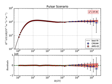
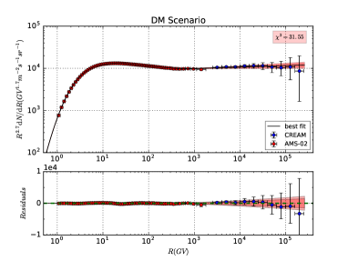
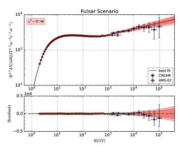
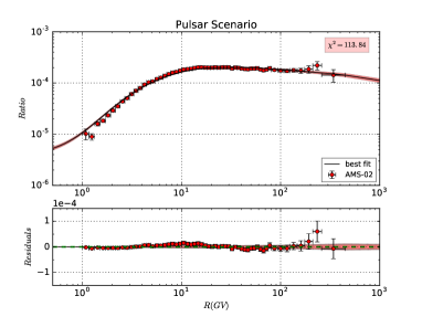
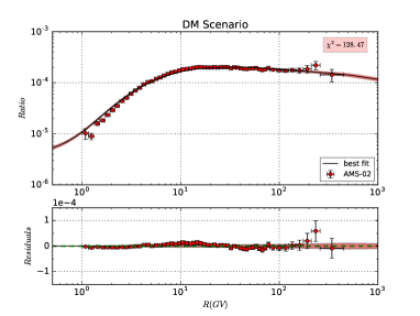
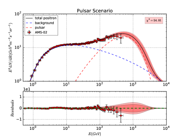
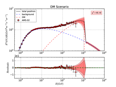
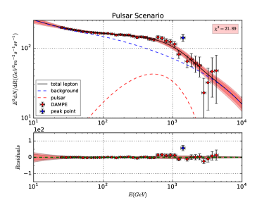
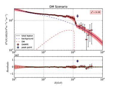
The MCMC algorithm was used to determine the parameters in the 2 scenarios. When the Markov Chains have reached their equilibrium state, we take the samples of the parameters as their posterior PDFs. The best-fitting results and the corresponding residuals of the proton flux, helium flux and $\,\bar{\text{p}}/\text{p}$ ratio for 2 scenarios are showed in Fig. 1, and the corresponding results of the positron and CREs flux are showed in Fig. 2. The best-fit values, statistical mean values, standard deviations and allowed intervals at $95\%$ CL for parameters in set $\boldsymbol{\theta}_{\,\mathrm{psr}}$ and $\boldsymbol{\theta}_{\,\mathrm{DM}}$ are shown in Table 1 and Table 2, respectively. For best fit results of the global fitting, we got $\chi^{2}/d.o.f=255.24/298$ for pulsar scenario and $\chi^{2}/d.o.f=276.56/296$ for DM scenario.

Figure 1: The global fitting results and the corresponding residuals to the proton flux, helium flux and $\,\bar{\text{p}}/\text{p}$ ratio for 2 scenarios. The $2\sigma$ (deep red) and $3\sigma$ (light red) bound are also showed in the figures.

ID	Prior	Best-fit	Posterior mean and	Posterior 95%
	range	value	Standard deviation	range
$D_{0}\ (10^{28}\,\mathrm{cm}^{2}\,\mathrm{s}^{-1})$	[1, 20]	14.37	14.38$\pm$0.16	[13.95, 14.74]
$\delta$	[0.1, 1.0]	0.318	0.317$\pm$0.003	[0.311, 0.326]
$z_{h}\ (\,\mathrm{kpc})$	[0.5, 30.0]	25.08	25.13$\pm$0.22	[24.55, 25.69]
$v_{A}\ (\,\mathrm{km}/\,\mathrm{s})$	[0, 80]	41.34	41.34$\pm$0.38	[40.37, 42.32]
$N_{p}\$	[1, 8]	4.46	4.46$\pm$0.01	[4.44, 4.49]
$R_{\,\mathrm{p}1}\ (\,\mathrm{GV})$	[1, 30]	25.88	25.78$\pm$0.20	[25.43, 26.41]
$R_{\,\mathrm{p}2}\ (\,\mathrm{GV})$	[60, 1000]	428.98	429.05$\pm$7.44	[409.86, 447.63]
$\nu_{\,\mathrm{p}1}$	[1.0, 4.0]	2.196	2.198$\pm$0.006	[2.180, 2.209]
$\nu_{\,\mathrm{p}2}$	[1.0, 4.0]	2.465	2.464$\pm$0.005	[2.453, 2.474]
$\nu_{\,\mathrm{p}3}$	[1.0, 4.0]	2.348	2.349$\pm$0.008	[2.332, 2.368]
$R_{\,\mathrm{He}1}\ (\,\mathrm{GV})$	[1, 30]	12.07	12.09$\pm$0.15	[11.67, 12.50]
$R_{\,\mathrm{He}2}\ (\,\mathrm{GV})$	[60, 1000]	244.83	246.41$\pm$8.14	[220.09, 265.47]
$\nu_{\,\mathrm{He}1}$	[1.0, 4.0]	2.186	2.188$\pm$0.007	[2.170, 2.199]
$\nu_{\,\mathrm{He}2}$	[1.0, 4.0]	2.422	2.422$\pm$0.005	[2.411, 2.431]
$\nu_{\,\mathrm{He}3}$	[1.0, 4.0]	2.219	2.219$\pm$0.012	[2.197, 2.241]
$\phi_{\mathrm{nuc}}\ (\,\mathrm{GV})$	[0, 1.5]	0.73	0.73$\pm$0.01	[0.71, 0.76]
$\phi_{\,\bar{\text{p}}}\ (\,\mathrm{GV})$	[0, 1.5]	0.28	0.28$\pm$0.01	[0.26, 0.30]
$c_{\,\mathrm{He}}$	[0.1, 10.0]	3.93	3.89$\pm$0.11	[3.66, 4.22]
$c_{\,\bar{\text{p}}}$	[0.1, 10.0]	1.37	1.37$\pm$0.02	[1.34, 1.41]
$\log(N_{\,\mathrm{e}})\$	[-4, 0]	-1.936	-1.936$\pm$0.006	[-1.950, -1.926]
$\log(R_{\,\mathrm{e}}/\,\mathrm{GV})$	[0, 3]	1.64	1.64$\pm$0.03	[1.55, 1.75]
$\nu_{\,\mathrm{e}1}$	[1.0, 4.0]	2.56	2.57$\pm$0.02	[2.50, 2.61]
$\nu_{\,\mathrm{e}2}$	[1.0, 4.0]	2.39	2.39$\pm$0.01	[2.36, 2.42]
$\log(N_{\,\mathrm{psr}})\$	[-8, -4]	-6.15	-6.15$\pm$0.02	[-6.19, -6.11]
$\nu_{\,\mathrm{psr}}$	[0, 3.0]	0.65	0.65$\pm$0.01	[0.61, 0.69]
$\log(R_{c}/\,\mathrm{GV}))$	[2, 5]	2.81	2.80$\pm$0.02	[2.78, 2.86]
$\phi_{e^{+}}\ (\,\mathrm{GV})$	[0, 1.5]	1.37	1.37$\pm$0.01	[1.36, 1.39]
$c_{e^{+}}$	[0.1, 10.0]	5.09	5.08$\pm$0.05	[5.03, 5.15]

Table 1: Constraints on the parameters in set $\boldsymbol{\theta}_{\,\mathrm{psr}}$. The prior interval, best-fit value, statistic mean, standard deviation and the allowed range at $95\%$ CL are listed for parameters. With $\chi^{2}/d.o.f=255.24/298$ for best fit result.

ID	Prior	Best-fit	Posterior mean and	Posterior 95%
	range	value	Standard deviation	range
$D_{0}\ (10^{28}\,\mathrm{cm}^{2}\,\mathrm{s}^{-1})$	[1, 20]	15.72	15.76$\pm$0.14	[15.47, 15.96]
$\delta$	[0.1, 1.0]	0.307	0.307$\pm$0.004	[0.302, 0.313]
$z_{h}\ (\,\mathrm{kpc})$	[0.5, 30.0]	28.59	28.39$\pm$0.22	[28.07, 28.78]
$v_{A}\ (\,\mathrm{km}/\,\mathrm{s})$	[0, 80]	42.46	42.60$\pm$0.48	[41.69, 43.32]
$N_{p}\$	[1, 8]	4.50	4.48$\pm$0.02	[4.45, 4.51]
$R_{\,\mathrm{p}1}\ (\,\mathrm{GV})$	[1, 30]	23.18	23.19$\pm$0.20	[22.92, 23.60]
$R_{\,\mathrm{p}2}\ (\,\mathrm{GV})$	[60, 1000]	497.28	492.08$\pm$8.41	[480.08, 507.07]
$\nu_{\,\mathrm{p}1}$	[1.0, 4.0]	2.222	2.226$\pm$0.009	[2.212, 2.239]
$\nu_{\,\mathrm{p}2}$	[1.0, 4.0]	2.477	2.477$\pm$0.006	[2.468, 2.486]
$\nu_{\,\mathrm{p}3}$	[1.0, 4.0]	2.357	2.352$\pm$0.009	[2.338, 2.368]
$R_{\,\mathrm{He}1}\ (\,\mathrm{GV})$	[1, 30]	11.06	11.23$\pm$0.17	[10.97, 11.57]
$R_{\,\mathrm{He}2}\ (\,\mathrm{GV})$	[60, 1000]	237.29	232.95$\pm$8.88	[219.91, 248.52]
$\nu_{\,\mathrm{He}1}$	[1.0, 4.0]	2.206	2.207$\pm$0.008	[2.196, 2.221]
$\nu_{\,\mathrm{He}2}$	[1.0, 4.0]	2.435	2.435$\pm$0.005	[2.426, 2.443]
$\nu_{\,\mathrm{He}3}$	[1.0, 4.0]	2.232	2.232$\pm$0.013	[2.213, 2.257]
$\phi_{\mathrm{nuc}}\ (\,\mathrm{GV})$	[0, 1.5]	0.77	0.78$\pm$0.01	[0.76, 0.80]
$\phi_{\,\bar{\text{p}}}\ (\,\mathrm{GV})$	[0, 1.5]	0.25	0.26$\pm$0.01	[0.24, 0.27]
$c_{\,\mathrm{He}}$	[0.1, 10.0]	3.68	3.56$\pm$0.11	[3.38, 3.74]
$c_{\,\bar{\text{p}}}$	[0.1, 10.0]	1.47	1.47$\pm$0.02	[1.44, 1.50]
$\log(N_{\,\mathrm{e}})\$	[-4, 0]	-1.940	-1.943$\pm$0.007	[-1.958, -1.928]
$\log(R_{\,\mathrm{e}}/\,\mathrm{GV})$	[0, 3]	1.62	1.63$\pm$0.04	[1.57, 1.74]
$\nu_{\,\mathrm{e}1}$	[1.0, 4.0]	2.55	2.54$\pm$0.03	[2.46, 2.60]
$\nu_{\,\mathrm{e}2}$	[1.0, 4.0]	2.37	2.37$\pm$0.01	[2.34, 2.40]
$\log(m_{\chi}/\,\mathrm{GeV})$	[1, 6]	3.082	3.085$\pm$0.006	[3.076, 3.096]
$\log(\langle\sigma v\rangle)$	[-28, -18]	-22.83	-22.80$\pm$0.06	[-22.93, -22.70]
$\eta_{e}$	[0, 1]	0.484	0.479$\pm$0.007	[0.466, 0.488]
$\eta_{\mu}$	[0, 1]	0.508	0.508$\pm$0.008	[0.493, 0.518]
$\eta_{\tau}$	[0, 1]	0.008	0.013$\pm$0.010	[0.001, 0.032]
$\phi_{e^{+}}\ (\,\mathrm{GV})$	[0, 1.5]	1.32	1.31$\pm$0.01	[1.296, 1.332]
$c_{e^{+}}$	[0.1, 10.0]	5.02	5.03$\pm$0.03	[4.97, 5.08]

Table 2: The same as Table. 1, but for the ones in set $\boldsymbol{\theta}_{\,\mathrm{DM}}$. With $\chi^{2}/d.o.f=276.56/296$ for best fit result.

In Fig. 1, we can see that the nuclei data is perfectly reproduced, which would provide a good precondition for the subsequent fitting on the lepton data. The proton and helium particles $\gtrsim\,\mathrm{TeV}$ would produce the secondary particles (including anti-protons and positrons) in lower energy range. Although the CREAM proton and helium data in $\gtrsim\,\mathrm{TeV}$ has a relative large uncertainties, the spectral hardening at $\sim 300\,\mathrm{GeV}$ is accounted and then its influence on secondary products is included.

The best-fitting results and the corresponding residuals of the lepton and positron spectra are showed in Fig. 2. The corresponding best-fit values, statistical mean values, standard deviations and allowed intervals at $95\%$ CL for these parameters are shown in Table 1 and Table 2.

In Fig. 2, the lepton data can be fitted within fitting uncertainties. Although we got smaller reduced $\chi^{2}$ from global fitting on pulsar scenario, if we consider the DAMPE CREs flux alone, the best fit results shows $\chi^{2}=21.89$ for pulsar scenario and $\chi^{2}=14.63$ for DM scenario.

Figure 2: The global fitting results and the corresponding residuals to the AMS-02 positron flux and DAMPE lepton flux. The $2\sigma$ (deep red) and $3\sigma$ (light red) bound are also showed in the figures. The first column shows the fitting results of pulsar and the second shows the fitting results of DM. For DAMPE CREs flux only, we got $\chi^{2}=21.89$ for pulsar scenario and $\chi^{2}=14.63$ for DM scenario.

IV.1 Propagation parameters

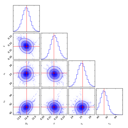
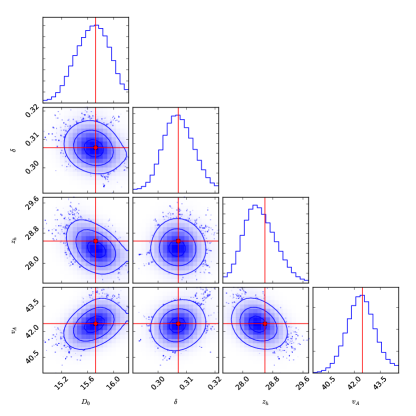
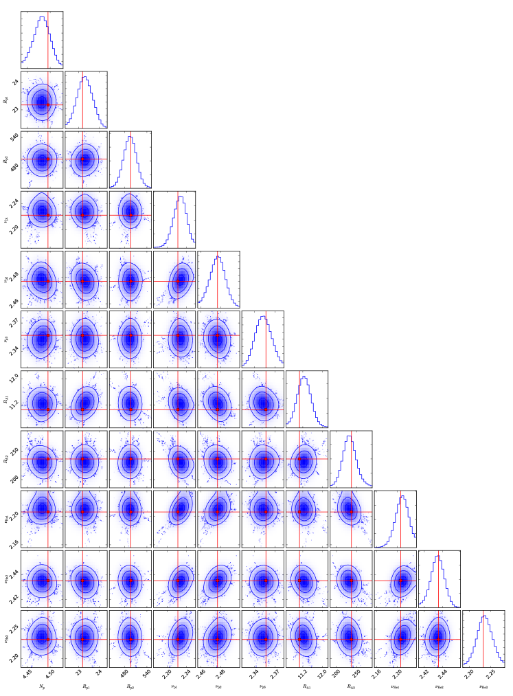
The results of posterior probability distributions of the propagation parameters are shown in Fig. 3 (for pulsar scenario) and Fig. 4 (for DM scenario).

In this work, we adapt the widely used diffusion-reacceleration model to describe the propagation process, and the relevant propagation parameter are $D_{0}$, $\delta$, $z_{h}$, and $v_{A}$. The obtained posterior PDFs are different from previous works to some extent. The classical degeneracy between $D_{0}$ and $z_{h}$ is not obvious due to the data set in this work, but both of them get larger best fit values than previous works. This is because (i) the $D_{0}$ defined in the dragon (which represents the perpendicular diffusion coefficient $D_{\perp}$) is not the same as that in galprop (which represents the isotropic diffusion coefficient); (ii) the sensitivity region which could breaks the degeneracy between $D_{0}$ and $z_{h}$ is different between $\,\bar{\text{p}}/\text{p}$ (10 - 100 GeV) and B/C ($\lesssim 10\,\mathrm{GeV}$). The observed AMS-02 $\,\bar{\text{p}}/\text{p}$ ratio favors larger $D_{0}$ and $z_{h}$ values.

The $\delta$ value obtained in this work is smaller than some of the previous works because we use one more break in the primary source injection of proton ($\sim 240\,\mathrm{GV}$) and helium ($\sim 420-500\,\mathrm{GV}$) to account for the observed hardening in their observed spectra, other than use only one break and let $\delta$ compromise the different slopes in high energy regions ($\gtrsim 240-500\,\mathrm{GV}$) (see, e.g., Niu and Li (2018)). In such configuration, we also got smaller fitting uncertainties on $\delta$ ($\sim 0.03$).

Moreover, the fitting results favor relative large values of $v_{A}$, which may not only comes from the constraints of nuclei data in low energy regions, but also the positron data as well.

Figure 3: Fitting 1D probability and 2D credible regions of posterior PDFs for the combinations of all propagation parameters for pulsar scenario. The regions enclosing $\sigma$, $2\sigma$ and $3\sigma$ CL are shown in step by step lighter blue. The red cross lines and marks in each plot indicates the best-fit value (largest likelihood).

Figure 4: Same as Fig. 3 but for DM scenario.

IV.2 Primary source injection parameters

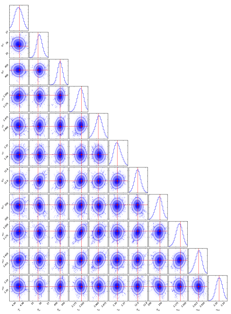
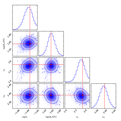
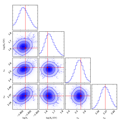
The results of posterior probability distributions of the primary source parameters are shown in Figs. 5 (proton and helium, for pulsar scenario), 6 (proton and helium, for DM scenario), and Figs. 7 (electron, for pulsar scenario), 8 (electron, for DM scenario).

Benefited from the 2 independent breaks injection spectra for proton and helium, the observed data has been reproduced perfectly. The fitting result shows that the rigidity breaks and the slopes are obviously different between proton and helium spectra. This indicates that the cosmic ray physics has entered a precision-driven era and all these differences should be treated carefully in future studies. On the other hand, we want to point out that the hardening of the nuclei spectra $\sim 300\,\mathrm{GeV}$ could also be reproduced by other proposals, which focus on the propagation and diffusion effects rather than ascribing it to the acceleration near the source. These solutions include proposing a spatial dependent diffusion coefficient (Tomassetti, 2012, 2015; Feng et al., 2016), or adding a high-rigidity break in the diffusion coefficient (Génolini et al., 2017; Blasi, 2017; Reinert and Winkler, 2018). With the precise data obtained in future extending to higher energy regions, we would expect more details can be revealed on this theme.

Additionally, the electron primary source injection spectra can be described by a break power-law from 20 GeV to $10^{4}$ GeV (DAMPE data), with $\nu_{\,\mathrm{e}1}\in[2.54,2.57]$, $\nu_{\,\mathrm{e}2}\in[2.37,2.39]$, and $R_{\,\mathrm{e}}\in[38,47]\,\mathrm{GV}$.

Figure 5: Fitting 1D probability and 2D credible regions of posterior PDFs for the combinations of nuclei primary source injection parameters for pulsar scenario. The regions enclosing $\sigma$, $2\sigma$ and $3\sigma$ CL are shown in step by step lighter blue. The red cross lines and marks in each plot indicates the best-fit value (largest likelihood).

Figure 6: Same as Fig. 5 but for DM scenario.

Figure 7: Fitting 1D probability and 2D credible regions of posterior PDFs for the combinations of electron primary source injection parameters for pulsar scenario. The regions enclosing $\sigma$, $2\sigma$ and $3\sigma$ CL are shown in step by step lighter blue. The red cross lines and marks in each plot indicates the best-fit value (largest likelihood).

Figure 8: Same as Fig. 7 but for DM scenario.

IV.3 Extra source parameters

The results for posterior probability distributions of the extra source parameters are shown in Figs. 9 (for pulsar scenario), 10 (for DM scenario).

Figure 9: Fitting 1D probability and 2D credible regions of posterior PDFs for the combinations of extra lepton soruce parameters from for pulsar scenario. The regions enclosing $\sigma$, $2\sigma$ and $3\sigma$ CL are shown in step by step lighter blue. The red cross lines and marks in each plot indicates the best-fit value (largest likelihood).

Figure 10: Same as Fig. 9 but for DM scenario.

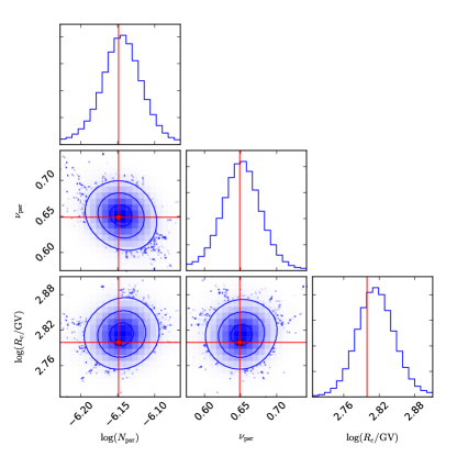
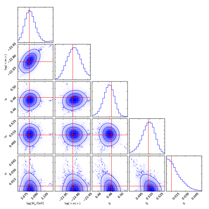
For the pulsar scenario, the fitting results give $\nu_{\,\mathrm{psr}}\simeq 0.65$, which is obviously different from the fitting results in previous works (see for e.g., (Profumo, 2012)). In standard pulsar models, the injection spectrum indices of CREs from pulsars are always in the range $\nu_{\,\mathrm{psr}}\in[1.0,2.4]$ (Reynolds, 1988; Thompson et al., 1994; Fierro et al., 1995). As a result, more attention should be paid in future researches. This may indicate: (i) there is something wrong or inaccuracy with the classical pulsar CRE injection model; (ii) the CRE excess is not contributed dominatly by pulsars. Moreover, the rigidity cut-off is $R_{c}\simeq 646$ GV.

For the DM scenario, we obtain $\langle\sigma v\rangle\simeq 1.48\times 10^{-23}\,\mathrm{cm}^{2}\,\mathrm{s}^{-1}$ and $m_{\chi}\simeq 1208\,\mathrm{GeV}$. The value of $\langle\sigma v\rangle$ is about 3 orders larger than that of thermal DM (Jungman et al., 1996). Moreover, we have $\eta_{e}\simeq 0.484$, $\eta_{\mu}\simeq 0.508$, and $\eta_{\tau}\simeq 0.008$, which is obviously different from the fitting results obtained from AMS-02 lepton data alone (see for e.g., Lin et al. (2015)). Consequently, the DM annihilation into $\tau\bar{\tau}$ is highly suppressed, which provides some hints to construct an appropriate DM model (see for e.g., (Chao et al., 2017)).

Because we have $\eta_{e}\simeq 0.484$, $\eta_{\mu}\simeq 0.508$, and $\eta_{\tau}\simeq 0.008$, the constraints from the Fermi-LAT observations on dwarf spheroidal galaxies (Ackermann et al., 2011; Geringer-Sameth and Koushiappas, 2011; Tsai et al., 2013; Ackermann et al., 2015; Li et al., 2016; Profumo et al., 2017) can be avoided (Yuan et al., 2017a). In order to escape the constraints from the Planck observations of CMB anisotropies (Ade et al., 2016), the Breit-Wigner mechanism (Feldman et al., 2009; Ibe et al., 2009; Guo and Wu, 2009; Bi et al., 2009, 2012; Hisano et al., 2011; Bai et al., 2017; Xiang et al., 2017) could be employed and the dark $U(1)_{D}$ model (where the SM fermions and Higgs fields are neutral under it) is considered. We introduce one SM singlet field $S$, one chiral fermionic dark matter particle $\chi$, and three pairs of the vector-like particles (${\widehat{XE}}_{i},{\widehat{XE}}_{i}^{c})$, whose quantum numbers under the $SU(3)_{C}\times SU(2)_{L}\times U(1)_{Y}\times U(1)_{D}$ are

$$S:(\mathbf{1},\mathbf{1},\mathbf{0},\mathbf{2})~{},~{}~{}~{}\chi:(\mathbf{1},\mathbf{1},\mathbf{0},\mathbf{-1})$$

$${\widehat{XE}}_{i}:(\mathbf{1},\mathbf{1},\mathbf{-1},\mathbf{-2})~{},~{}~{}~{}{\widehat{XE}}^{c}_{i}:(\mathbf{1},\mathbf{1},\mathbf{1},\mathbf{2})~{}.~{}\,$$ (6)

The relevant Lagrangian is

$$-{\cal L} = -m_{S}^{2}|S|^{2}+\frac{\lambda}{2}|S|^{4}+\left(M^{V}_{ij}{\widehat{XE}}^{c}_{i}{\widehat{XE}}_{j}\right.$$ (7)

$$\left.+y_{ij}S{\widehat{E}}_{i}^{c}{\widehat{XE}}_{j}+yS\chi\chi+{\rm H.C.}\right)~{},~{}\,$$

where ${\widehat{E}}_{i}^{c}$ are the right-handed charged leptons.

For simplicity, we choose $M^{V}_{ij}=M^{V}_{i}\delta_{ij}$ and $y_{ij}=y_{i}\delta_{ij}$. After $S$ acquires a Vacuum Expectation Value (VEV), the $U(1)_{D}$ gauge symmetry is broken down to a $Z_{2}$ symmetry under which $\chi$ is odd. Thus, $\chi$ is a DM matter candidate. For simplicity, we assume that the mass of $U(1)_{D}$ gauge boson is about twice of $\chi$ mass, i.e., $M_{Z^{\prime}}\simeq 2m_{\chi}$, while the Higgs field $S$ and vector-like particles are heavier than $M_{Z^{\prime}}$. Moreover, ${\widehat{E}}_{i}^{c}$ and ${\widehat{XE}}_{i}^{c}$ will be mixed due to the $M^{V}_{i}{\widehat{XE}}^{c}_{i}{\widehat{XE}}_{i}$ and $y_{i}S{\widehat{E}}_{i}^{c}{\widehat{XE}}_{i}$ terms, and we obtain the mass eigenstates $E_{i}^{c}$ and $XE_{i}^{c}$ by neglecting the tiny charged lepton masses

$$\left(\begin{array}[]{c}E_{i}^{c}\\ XE_{i}^{c}\end{array}\right)=\left(\begin{array}[]{cc}\cos\theta_{i}&\sin\theta_{i}\\ -\sin\theta_{i}&\cos\theta_{i}\end{array}\right)\left(\begin{array}[]{c}{\widehat{E}}_{i}^{c}\\ {\widehat{XE}}_{i}^{c\prime}\end{array}\right)~{},~{}\,$$ (14)

where $\tan\theta_{i}=-y\langle S\rangle/M^{V}_{i}$.

Neglecting the charged lepton masses again, we obtain

$$\sigma v=\sum_{i=1}^{3}\frac{g^{\prime 4}\sin^{2}\theta_{i}}{6\pi}\frac{s-m_{\chi}^{2}}{(s-m_{Z^{\prime}}^{2})^{2}+(m_{Z^{\prime}}\Gamma_{Z^{\prime}})^{2}}~{},~{}\,$$ (15)

where $m_{\chi}=y\langle S\rangle$, and $g^{\prime}$ and $M_{Z^{\prime}}$ are the gauge coupling and gauge boson mass for $U(1)_{D}$ gauge symmetry.

For $m_{Z^{\prime}}\simeq 2m_{\chi}$, $Z^{\prime}$ decays dominantly into leptons, and the decay width is

$$\Gamma_{Z^{\prime}}=\sum_{i=1}^{3}\frac{g^{\prime 2}\sin^{2}\theta_{i}}{6\pi}m_{Z^{\prime}}~{}.~{}\,$$ (16)

To explain the DM best fit results, we can choose proper values of $g^{\prime}$, $\frac{m_{Z^{\prime}}-2m_{\chi}}{m_{Z^{\prime}}}$, $\sin\theta_{e}$, $\sin\theta_{\mu}$, and $\sin\theta_{\tau}$ to reproduce the values of $m_{\chi}$, $\langle\sigma v\rangle$ and $\eta_{e}:\eta_{\mu}:\eta_{\tau}$ like that in Niu et al. (2017).

IV.4 Nuisance parameters

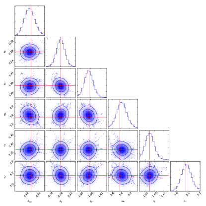
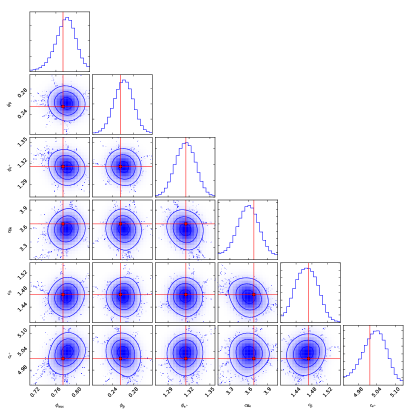
In Figs 11 and 12, the results of posterior probability distributions represent the necessity to introduce them in the global fitting.

The different values of $\phi_{\mathrm{nuc}}$, $\phi_{\,\bar{\text{p}}}$, and $\phi_{e^{+}}$ from the best-fit results represent not only the charge-sign dependent solar modulation (which has also been claimed by some previous works, see, e.g., Clem et al. (1996); Boella et al. (2001); Niu and Li (2018)), but also a species dependent solar modulation to some extent. As claimed in our previous works (Niu and Li, 2018), the force field approximation could not describe the effects of solar modulation to all the species by a single $\phi$, but as an effective model, we can use an independent $\phi$ for each of the species. The different values of the $\phi$s for different species could reveal the hints to improve the propagation mechanisms of them in the heliosphere. Additionally, the proton, helium, and positron data have been collected from AMS-02 in the same period with a suggested $\phi$ from 0.50 - 0.62 GV (AMS collaboration et al., 2015a, b, 2014c), which is based on data from the world network of sea level neutron monitors (Usoskin et al., 2011). More details in this field can be gotten in Corti et al. (2016).

The value of $c_{\,\bar{\text{p}}}\sim 1.4-1.5$ could be explained by the uncertainties on the antiproton production cross section (Tan and Ng, 1983; Duperray et al., 2003; Kappl and Winkler, 2014; di Mauro et al., 2014; Lin et al., 2017).

The dragon primary source isotopic abundances are inherited from galprop, which are taken as the solar system abundances and iterated to achieve and agreement with the propagated abundances as provided by ACE at $\sim 200\,\mathrm{MeV}$ nucleon. It is naturally that the normalized factor is different in different energy regions. On the other hand, we always focus on the shape of the spectrum, and $c_{\,\mathrm{He}}$ could be considered as an independent normalized factor as $N_{p}$, which is just identified as an nuisance parameter to get a better fitting result and not that important in this work.

For $c_{e^{+}}$, there are several reasons which could ascribe its relative large values: (i) the cross section comes from Kamae et al. (2005, 2006), which needed a scale factor to correlate its values (Evoli et al., 2017); (ii) the systematics between DAMPE CREs spectrum and AMS-02 positron spectrum is also partially accounted for in the parameter $c_{e^{+}}$, which lead $c_{e^{+}}$ not just a indicator of rescale factor on cross section. Moreover, we would like to point our that in this work, we focus on the extra sources which would reproduce the break at $\sim 1\,\mathrm{TeV}$ in DAMPE CREs data. Some nuisance parameters ($c_{\,\bar{\text{p}}}$, $c_{\,\mathrm{He}}$, and $c_{e^{+}}$) are employed to fit all the data consistently and precisely (especially the primary source and background, see for e.g., Lin et al. (2015)), which may not have clear physical meanings, but could also give us some hints to improve the details in CR physics in future research.

Figure 11: Fitting 1D probability and 2D credible regions of posterior PDFs for the combinations of nuisance parameters for pulsar scenario. The regions enclosing $\sigma$, $2\sigma$ and $3\sigma$ CL are shown in step by step lighter blue. The red cross lines and marks in each plot indicates the best-fit value (largest likelihood).

Figure 12: Same as Fig. 11 but for DM scenario.

V Conclusion

In this work, we did Bayesian analysis on the newly released CREs flux (exclude the peak signal at $\sim 1.4\,\mathrm{TeV}$) from DAMPE to study the extra source properties in it. In order to deduct the primary electrons, secondary leptons in CREs flux consistently and precisely, we did a global fitting to reproduce the proton flux (from AMS-02 and CREAM), helium flux (from AMS-02 and CREAM), $\,\bar{\text{p}}/\text{p}$ ratio (from AMS-02), positron flux (from AMS-02) and CREs flux (from DAMPE) simultaneously. Two independent extra source scenarios are considered, which account the excess of leptons to continuously distributed pulsars in the galaxy and dark matter annihilation (via leptonic channels) in the galactic halo. Both of these scenarios can fit the DAMPE CREs flux within the fitting uncertainties, while DM scenario gave a smaller $\chi^{2}$ and a obvious break at $\sim 1\,\mathrm{TeV}$.

Additionally, in the DM scenario, the fitting result gives a dark matter particle’s mass $m_{\chi}\sim 1208\,\mathrm{GeV}$ and a cross section $\langle\sigma v\rangle\sim 1.48\times 10^{-23}\,\mathrm{cm}^{3}\,\mathrm{s}^{-1}$. This is benefited from the break at $\sim 1\,\mathrm{TeV}$. In such situations, the cross section in this work still should have a suppress factor to meet the value $\langle\sigma v\rangle\sim 3\times 10^{-26}\,\mathrm{cm}^{3}\,\mathrm{s}^{-1}$. This discrepancy can be resolved by some proposed mechanisms like the non-thermal production of the DM (Jeannerot et al., 1999; Lin et al., 2001; Yuan et al., 2012), the Sommerfeld enhancement mechanism (Sommerfeld, 1931; Hisano et al., 2005; Arkani-Hamed et al., 2009), and Breit-Wigner type resonance of the annihilation interaction (Griest and Seckel, 1991; Gondolo and Gelmini, 1991). What’s more interesting, the constraints on the annihilation branching fraction shows the $\tau\bar{\tau}$ annihilation channel is strongly suppressed, while the $e^{-}e^{+}$ and $\mu\bar{\mu}$ channels are almost equally weighted ($\eta_{e}=0.484$, $\eta_{\mu}=0.508$, and $\eta_{\tau}=0.008$). This would give some hints for constructing DM models, and we tried to build one in this work to meet the fitting results.

Note: In this work, we can see that the CREs spectrum from DAMPE without the peak can be reproduced by DM scenarios precisely. On the other hand, the spectrum with the peak also can be reproduced by DM annihilation from a local DM sub-structure (Yuan et al., 2017a; Athron et al., 2017; Fan et al., 2017; Duan et al., 2017; Gu and He, 2017; Liu and Liu, 2017; Cao et al., 2017; Jin et al., 2017; Huang et al., 2017; Yang et al., 2017; Ge and He, 2017). Both of these situations call for DM particles with $m_{\chi}\sim 1-2\,\mathrm{TeV}$. Other independent detection strategy is needed to distinguish the excess in the CREs spectrum which can also be produced from some astrophysical sources (Fang et al., 2017; Yuan et al., 2017a; Cholis et al., 2017). Our recent works (Niu et al., 2017) proposed a novel scenario to probe the interaction between DM particles and electrons with $5\,\mathrm{GeV}\lesssim m_{\chi}\lesssim 10\,\mathrm{TeV}$.

References

- Chang (2014) J. Chang, “Dark matter particle explorer: The first chinese cosmic ray and hard gamma-ray detector in space,” Chinese Journal of Space Science 34, 550 (2014).
- Chang et al. (2017) J. Chang et al. (DAMPE), “The DArk Matter Particle Explorer mission,” Astropart. Phys. 95, 6–24 (2017), arXiv:1706.08453 [astro-ph.IM] .
- Ambrosi et al. (2017) G. Ambrosi et al. (DAMPE), “Direct detection of a break in the teraelectronvolt cosmic-ray spectrum of electrons and positrons,” Nature (2017), 10.1038/nature24475, arXiv:1711.10981 [astro-ph.HE] .
- Adriani et al. (2009) O. Adriani, G. C. Barbarino, G. A. Bazilevskaya, R. Bellotti, M. Boezio, E. A. Bogomolov, L. Bonechi, M. Bongi, V. Bonvicini, S. Bottai, and et al., “An anomalous positron abundance in cosmic rays with energies 1.5-100GeV,” Nature 458, 607–609 (2009), arXiv:0810.4995 .
- PAMELA collaboration et al. (2010) PAMELA collaboration, O. Adriani, G. C. Barbarino, G. A. Bazilevskaya, R. Bellotti, M. Boezio, E. A. Bogomolov, L. Bonechi, M. Bongi, V. Bonvicini, S. Borisov, and el al., “A statistical procedure for the identification of positrons in the PAMELA experiment,” Astroparticle Physics 34, 1–11 (2010), arXiv:1001.3522 [astro-ph.HE] .
- AMS collaboration et al. (2014a) AMS collaboration, M. Aguilar, D. Aisa, B. Alpat, A. Alvino, G. Ambrosi, K. Andeen, L. Arruda, N. Attig, P. Azzarello, A. Bachlechner, and et al., “Precision Measurement of the (e++e-) Flux in Primary Cosmic Rays from 0.5 GeV to 1 TeV with the Alpha Magnetic Spectrometer on the International Space Station,” Physical Review Letters 113, 221102 (2014a).
- Fermi-LAT collaboration et al. (2012) Fermi-LAT collaboration, M. Ackermann, M. Ajello, A. Allafort, W. B. Atwood, L. Baldini, G. Barbiellini, D. Bastieri, K. Bechtol, R. Bellazzini, B. Berenji, and el al., “Measurement of Separate Cosmic-Ray Electron and Positron Spectra with the Fermi Large Area Telescope,” Physical Review Letters 108, 011103 (2012), arXiv:1109.0521 [astro-ph.HE] .
- collaboration et al. (2017a) CALET collaboration, O. Adriani, Y. Akaike, K. Asano, Y. Asaoka, M. G. Bagliesi, G. Bigongiari, W. R. Binns, S. Bonechi, M. Bongi, P. Brogi, and et al., “Energy spectrum of cosmic-ray electron and positron from 10 gev to 3 tev observed with the calorimetric electron telescope on the international space station,” Phys. Rev. Lett. 119, 181101 (2017a).
- collaboration et al. (2017b) Fermi-LAT collaboration, S. Abdollahi, M. Ackermann, M. Ajello, W. B. Atwood, L. Baldini, G. Barbiellini, D. Bastieri, R. Bellazzini, E. D. Bloom, and et al., “Cosmic-ray electron-positron spectrum from 7 gev to 2 tev with the fermi large area telescope,” Phys. Rev. D 95, 082007 (2017b).
- Malyshev et al. (2009) D. Malyshev, I. Cholis, and J. Gelfand, “Pulsars versus dark matter interpretation of ATIC/PAMELA,” Phys. Rev. D 80, 063005 (2009), arXiv:0903.1310 [astro-ph.HE] .
- Kuhlen and Malyshev (2009) M. Kuhlen and D. Malyshev, “ATIC, PAMELA, HESS, and Fermi data and nearby dark matter subhalos,” Phys. Rev. D 79, 123517 (2009), arXiv:0904.3378 [hep-ph] .
- Brun et al. (2009) P. Brun, T. Delahaye, J. Diemand, S. Profumo, and P. Salati, “Cosmic ray lepton puzzle in the light of cosmological N-body simulations,” Phys. Rev. D 80, 035023 (2009), arXiv:0904.0812 [astro-ph.HE] .
- Gendelev et al. (2010) L. Gendelev, S. Profumo, and M. Dormody, “The contribution of Fermi gamma-ray pulsars to the local flux of cosmic-ray electrons and positrons,” J. Cosmol. Astropart. Phys. 2, 016 (2010), arXiv:1001.4540 [astro-ph.HE] .
- Profumo (2012) S. Profumo, “Dissecting cosmic-ray electron-positron data with Occam’s razor: the role of known pulsars,” Central European Journal of Physics 10, 1–31 (2012), arXiv:0812.4457 .
- Panov (2013) A. D. Panov, “Electrons and Positrons in Cosmic Rays,” in Journal of Physics Conference Series, Journal of Physics Conference Series, Vol. 409 (2013) p. 012004, arXiv:1303.6118 [astro-ph.HE] .
- Fang et al. (2017) K. Fang, X.-J. Bi, and P.-F. Yin, “Explanation of the knee-like feature in the DAMPE cosmic energy spectrum,” ArXiv e-prints (2017), arXiv:1711.10996 [astro-ph.HE] .
- Yuan et al. (2017a) Q. Yuan, L. Feng, P.-F. Yin, Y.-Z. Fan, X.-J. Bi, M.-Y. Cui, T.-K. Dong, Y.-Q. Guo, K. Fang, H.-B. Hu, X. Huang, S.-J. Lei, X. Li, S.-J. Lin, H. Liu, P.-X. Ma, W.-X. Peng, R. Qiao, Z.-Q. Shen, M. Su, Y.-F. Wei, Z.-L. Xu, C. Yue, J.-J. Zang, C. Zhang, X. Zhang, Y.-P. Zhang, Y.-J. Zhang, and Y.-L. Zhang, “Interpretations of the DAMPE electron data,” ArXiv e-prints (2017a), arXiv:1711.10989 [astro-ph.HE] .
- Athron et al. (2017) P. Athron, C. Balazs, A. Fowlie, and Y. Zhang, “Model-independent analysis of the DAMPE excess,” ArXiv e-prints (2017), arXiv:1711.11376 [hep-ph] .
- Fan et al. (2017) Y.-Z. Fan, W.-C. Huang, M. Spinrath, Y.-L. Sming Tsai, and Q. Yuan, “A model explaining neutrino masses and the DAMPE cosmic ray electron excess,” ArXiv e-prints (2017), arXiv:1711.10995 [hep-ph] .
- Duan et al. (2017) G. H. Duan, L. Feng, F. Wang, L. Wu, J. M. Yang, and R. Zheng, “Simplified TeV leptophilic dark matter in light of DAMPE data,” ArXiv e-prints (2017), arXiv:1711.11012 [hep-ph] .
- Gu and He (2017) P.-H. Gu and X.-G. He, “Electrophilic dark matter with dark photon: from DAMPE to direct detection,” ArXiv e-prints (2017), arXiv:1711.11000 [hep-ph] .
- Liu and Liu (2017) X. Liu and Z. Liu, “TeV dark matter and the DAMPE electron excess,” ArXiv e-prints (2017), arXiv:1711.11579 [hep-ph] .
- Cao et al. (2017) J. Cao, L. Feng, X. Guo, L. Shang, F. Wang, and P. Wu, “Scalar dark matter interpretation of the DAMPE data with U(1) gauge interactions,” ArXiv e-prints (2017), arXiv:1711.11452 [hep-ph] .
- Profumo et al. (2017) S. Profumo, F. S. Queiroz, J. Silk, and C. Siqueira, “Searching for Secluded Dark Matter with H.E.S.S., Fermi-LAT, and Planck,” ArXiv e-prints (2017), arXiv:1711.03133 [hep-ph] .
- AMS collaboration et al. (2013a) AMS collaboration, M. Aguilar, G. Alberti, B. Alpat, A. Alvino, G. Ambrosi, K. Andeen, H. Anderhub, L. Arruda, P. Azzarello, A. Bachlechner, and et al., “First Result from the Alpha Magnetic Spectrometer on the International Space Station: Precision Measurement of the Positron Fraction in Primary Cosmic Rays of 0.5-350 GeV,” Physical Review Letters 110, 141102 (2013a).
- Barwick et al. (1997) S. W. Barwick, J. J. Beatty, A. Bhattacharyya, C. R. Bower, C. J. Chaput, S. Coutu, G. A. de Nolfo, J. Knapp, D. M. Lowder, S. McKee, D. Mueller, J. A. Musser, S. L. Nutter, E. Schneider, S. P. Swordy, G. Tarle, A. D. Tomasch, E. Torbet, and HEAT collaboration, “Measurements of the Cosmic-Ray Positron Fraction from 1 to 50 GeV,” Astrophys. J. Lett. 482, L191–L194 (1997), astro-ph/9703192 .
- AMS-01 collaboration (2007) AMS-01 collaboration, “Cosmic-ray positron fraction measurement from 1 to 30 GeV with AMS-01,” Physics Letters B 646, 145–154 (2007), astro-ph/0703154 .
- AMS collaboration et al. (2013b) AMS collaboration, M. Aguilar, G. Alberti, B. Alpat, A. Alvino, G. Ambrosi, K. Andeen, H. Anderhub, L. Arruda, P. Azzarello, A. Bachlechner, and et al., “First Result from the Alpha Magnetic Spectrometer on the International Space Station: Precision Measurement of the Positron Fraction in Primary Cosmic Rays of 0.5-350 GeV,” Physical Review Letters 110, 141102 (2013b).
- AMS collaboration et al. (2014b) AMS collaboration, L. Accardo, M. Aguilar, D. Aisa, A. Alvino, G. Ambrosi, K. Andeen, L. Arruda, N. Attig, P. Azzarello, A. Bachlechner, and et al., “High Statistics Measurement of the Positron Fraction in Primary Cosmic Rays of 0.5-500 GeV with the Alpha Magnetic Spectrometer on the International Space Station,” Physical Review Letters 113, 121101 (2014b).
- AMS collaboration et al. (2014c) AMS collaboration, M. Aguilar, D. Aisa, A. Alvino, G. Ambrosi, K. Andeen, L. Arruda, N. Attig, P. Azzarello, A. Bachlechner, F. Barao, and et al., “Electron and Positron Fluxes in Primary Cosmic Rays Measured with the Alpha Magnetic Spectrometer on the International Space Station,” Physical Review Letters 113, 121102 (2014c).
- Shen (1970) C. S. Shen, “Pulsars and Very High-Energy Cosmic-Ray Electrons,” Astrophys. J. Lett. 162, L181 (1970).
- Zhang and Cheng (2001) L. Zhang and K. S. Cheng, “Cosmic-ray positrons from mature gamma-ray pulsars,” Astron. Astrophys. 368, 1063–1070 (2001).
- Yüksel et al. (2009) H. Yüksel, M. D. Kistler, and T. Stanev, “TeV Gamma Rays from Geminga and the Origin of the GeV Positron Excess,” Physical Review Letters 103, 051101 (2009), arXiv:0810.2784 .
- Hooper et al. (2009) D. Hooper, P. Blasi, and P. Dario Serpico, “Pulsars as the sources of high energy cosmic ray positrons,” J. Cosmol. Astropart. Phys. 1, 025 (2009), arXiv:0810.1527 .
- Blasi (2009) P. Blasi, “Origin of the Positron Excess in Cosmic Rays,” Physical Review Letters 103, 051104 (2009), arXiv:0903.2794 [astro-ph.HE] .
- Hu et al. (2009) H.-B. Hu, Q. Yuan, B. Wang, C. Fan, J.-L. Zhang, and X.-J. Bi, “On the e+e- Excesses and the Knee of the Cosmic Ray Spectra Hints of Cosmic Ray Acceleration in Young Supernova Remnants,” Astrophys. J. Lett. 700, L170–L173 (2009), arXiv:0901.1520 [astro-ph.HE] .
- Fujita et al. (2009) Y. Fujita, K. Kohri, R. Yamazaki, and K. Ioka, “Is the PAMELA anomaly caused by supernova explosions near the Earth?” Phys. Rev. D 80, 063003 (2009), arXiv:0903.5298 [astro-ph.HE] .
- Bergström et al. (2008) L. Bergström, T. Bringmann, and J. Edsjö, “New positron spectral features from supersymmetric dark matter: A way to explain the PAMELA data?” Phys. Rev. D 78, 103520 (2008), arXiv:0808.3725 .
- Barger et al. (2009) V. Barger, W.-Y. Keung, D. Marfatia, and G. Shaughnessy, “PAMELA and dark matter,” Physics Letters B 672, 141–146 (2009), arXiv:0809.0162 [hep-ph] .
- Cirelli et al. (2009) M. Cirelli, M. Kadastik, M. Raidal, and A. Strumia, “Model-independent implications of the e+, e-, anti-proton cosmic ray spectra on properties of Dark Matter,” Nuclear Physics B 813, 1–21 (2009), arXiv:0809.2409 [hep-ph] .
- Zhang et al. (2009) J. Zhang, X.-J. Bi, J. Liu, S.-M. Liu, P.-F. Yin, Q. Yuan, and S.-H. Zhu, “Discriminating different scenarios to account for the cosmic e± excess by synchrotron and inverse Compton radiation,” Phys. Rev. D 80, 023007 (2009), arXiv:0812.0522 .
- Bergström et al. (2009) L. Bergström, J. Edsjö, and G. Zaharijas, “Dark Matter Interpretation of Recent Electron and Positron Data,” Physical Review Letters 103, 031103 (2009), arXiv:0905.0333 [astro-ph.HE] .
- Yin et al. (2013) P.-F. Yin, Z.-H. Yu, Q. Yuan, and X.-J. Bi, “Pulsar interpretation for the AMS-02 result,” Phys. Rev. D 88, 023001 (2013), arXiv:1304.4128 [astro-ph.HE] .
- Dev et al. (2014) P. S. B. Dev, D. K. Ghosh, N. Okada, and I. Saha, “Neutrino mass and dark matter in light of recent AMS-02 results,” Phys. Rev. D 89, 095001 (2014), arXiv:1307.6204 [hep-ph] .
- Lewis and Bridle (2002) A. Lewis and S. Bridle, “Cosmological parameters from CMB and other data: A Monte Carlo approach,” Phys. Rev. D 66, 103511 (2002), astro-ph/0205436 .
- Liu et al. (2010) J. Liu, Q. Yuan, X. Bi, H. Li, and X. Zhang, “Markov chain Monte Carlo study on dark matter property related to the cosmic e± excesses,” Phys. Rev. D 81, 023516 (2010), arXiv:0906.3858 [astro-ph.CO] .
- Lin et al. (2015) Su-Jie Lin, Qiang Yuan, and Xiao-Jun Bi, “Quantitative study of the ams-02 electron/positron spectra: implications for the pulsar and dark matter properties,” Physical Review D 91, 063508 (2015), arXiv:1409.6248 [astro-ph.HE] .
- Yuan et al. (2017b) Q. Yuan, S.-J. Lin, K. Fang, and X.-J. Bi, “Propagation of cosmic rays in the AMS-02 era,” ArXiv e-prints (2017b), arXiv:1701.06149 [astro-ph.HE] .
- Niu and Li (2018) J.-S. Niu and T. Li, “Galactic cosmic-ray model in the light of AMS-02 nuclei data,” Phys. Rev. D 97, 023015 (2018), arXiv:1705.11089 [astro-ph.HE] .
- Panov et al. (2006) A. D. Panov, J. H. Adams, H. S. Ahn, G. L. Bashindzhagyan, K. E. Batkov, J. Chang, M. Christl, A. R. Fazely, O. Ganel, R. M. Gunashingha, T. G. Guzik, J. Isbert, K. C. Kim, E. N. Kouznetsov, M. I. Panasyuk, W. K. H. Schmidt, E. S. Seo, N. V. Sokolskaya, J. W. Watts, J. P. Wefel, J. Wu, and V. I. Zatsepin, “The results of ATIC-2 experiment for elemental spectra of cosmic rays,” ArXiv Astrophysics e-prints (2006), astro-ph/0612377 .
- Ahn et al. (2010) H. S. Ahn, P. Allison, M. G. Bagliesi, J. J. Beatty, G. Bigongiari, J. T. Childers, N. B. Conklin, S. Coutu, M. A. DuVernois, O. Ganel, J. H. Han, J. A. Jeon, K. C. Kim, M. H. Lee, L. Lutz, P. Maestro, A. Malinin, P. S. Marrocchesi, S. Minnick, S. I. Mognet, J. Nam, S. Nam, S. L. Nutter, I. H. Park, N. H. Park, E. S. Seo, R. Sina, J. Wu, J. Yang, Y. S. Yoon, R. Zei, and S. Y. Zinn, “Discrepant Hardening Observed in Cosmic-ray Elemental Spectra,” Astrophys. J. Lett. 714, L89–L93 (2010), arXiv:1004.1123 [astro-ph.HE] .
- PAMELA collaboration et al. (2011a) PAMELA collaboration, O. Adriani, G. C. Barbarino, G. A. Bazilevskaya, R. Bellotti, M. Boezio, E. A. Bogomolov, L. Bonechi, M. Bongi, V. Bonvicini, S. Borisov, and el al., “PAMELA Measurements of Cosmic-Ray Proton and Helium Spectra,” Science 332, 69 (2011a), arXiv:1103.4055 [astro-ph.HE] .
- AMS collaboration et al. (2015a) AMS collaboration, M. Aguilar, D. Aisa, B. Alpat, A. Alvino, G. Ambrosi, K. Andeen, L. Arruda, N. Attig, P. Azzarello, A. Bachlechner, and et al., “Precision Measurement of the Proton Flux in Primary Cosmic Rays from Rigidity 1 GV to 1.8 TV with the Alpha Magnetic Spectrometer on the International Space Station,” Physical Review Letters 114, 171103 (2015a).
- AMS collaboration et al. (2015b) AMS collaboration, M. Aguilar, D. Aisa, B. Alpat, A. Alvino, G. Ambrosi, K. Andeen, L. Arruda, N. Attig, P. Azzarello, A. Bachlechner, and et al., “Precision Measurement of the Helium Flux in Primary Cosmic Rays of Rigidities 1.9 GV to 3 TV with the Alpha Magnetic Spectrometer on the International Space Station,” Physical Review Letters 115, 211101 (2015b).
- Korsmeier and Cuoco (2016) M. Korsmeier and A. Cuoco, “Galactic cosmic-ray propagation in the light of AMS-02: I. Analysis of protons, helium, and antiprotons,” ArXiv e-prints (2016), arXiv:1607.06093 [astro-ph.HE] .
- Strong et al. (2000) A. W. Strong, I. V. Moskalenko, and O. Reimer, “Diffuse Continuum Gamma Rays from the Galaxy,” Astrophys. J. 537, 763–784 (2000), astro-ph/9811296 .
- PAMELA collaboration et al. (2011b) PAMELA collaboration, O. Adriani, G. C. Barbarino, G. A. Bazilevskaya, R. Bellotti, M. Boezio, E. A. Bogomolov, L. Bonechi, M. Bongi, V. Bonvicini, S. Borisov, and el al., “PAMELA Measurements of Cosmic-Ray Proton and Helium Spectra,” Science 332, 69 (2011b), arXiv:1103.4055 [astro-ph.HE] .
- Tan and Ng (1983) L. C. Tan and L. K. Ng, “Parametrisation of hadron inclusive cross sections in p-p collisions extended to very low energies,” Journal of Physics G Nuclear Physics 9, 1289–1308 (1983).
- Duperray et al. (2003) R. P. Duperray, C.-Y. Huang, K. V. Protasov, and M. Buénerd, “Parametrization of the antiproton inclusive production cross section on nuclei,” Phys. Rev. D 68, 094017 (2003), astro-ph/0305274 .
- Kappl and Winkler (2014) R. Kappl and M. W. Winkler, “The cosmic ray antiproton background for AMS-02,” J. Cosmol. Astropart. Phys. 9, 051 (2014), arXiv:1408.0299 [hep-ph] .
- di Mauro et al. (2014) M. di Mauro, F. Donato, A. Goudelis, and P. D. Serpico, “New evaluation of the antiproton production cross section for cosmic ray studies,” Phys. Rev. D 90, 085017 (2014), arXiv:1408.0288 [hep-ph] .
- Delahaye et al. (2009) T. Delahaye, R. Lineros, F. Donato, N. Fornengo, J. Lavalle, P. Salati, and R. Taillet, “Galactic secondary positron flux at the Earth,” Astron. Astrophys. 501, 821–833 (2009), arXiv:0809.5268 .
- Mori (2009) M. Mori, “Nuclear enhancement factor in calculation of Galactic diffuse gamma-rays: A new estimate with DPMJET-3,” Astroparticle Physics 31, 341–343 (2009), arXiv:0903.3260 [astro-ph.HE] .
- Cirelli et al. (2011) M. Cirelli, G. Corcella, A. Hektor, G. Hütsi, M. Kadastik, P. Panci, M. Raidal, F. Sala, and A. Strumia, “PPPC 4 DM ID: a poor particle physicist cookbook for dark matter indirect detection,” J. Cosmol. Astropart. Phys. 3, 051 (2011), arXiv:1012.4515 [hep-ph] .
- Ciafaloni et al. (2011) P. Ciafaloni, D. Comelli, A. Riotto, F. Sala, A. Strumia, and A. Urbano, “Weak corrections are relevant for dark matter indirect detection,” J. Cosmol. Astropart. Phys. 3, 019 (2011), arXiv:1009.0224 [hep-ph] .
- Navarro et al. (2004) J. F. Navarro, E. Hayashi, C. Power, A. R. Jenkins, C. S. Frenk, S. D. M. White, V. Springel, J. Stadel, and T. R. Quinn, “The inner structure of CDM haloes - III. Universality and asymptotic slopes,” Mon. Not. Roy. Astron. Soc. 349, 1039–1051 (2004), astro-ph/0311231 .
- Merritt et al. (2006) D. Merritt, A. W. Graham, B. Moore, J. Diemand, and B. Terzić, “Empirical Models for Dark Matter Halos. I. Nonparametric Construction of Density Profiles and Comparison with Parametric Models,” Astron. J. 132, 2685–2700 (2006), astro-ph/0509417 .
- Einasto (2009) J. Einasto, “Dark Matter,” ArXiv e-prints (2009), arXiv:0901.0632 [astro-ph.CO] .
- Navarro et al. (2010) J. F. Navarro, A. Ludlow, V. Springel, J. Wang, M. Vogelsberger, S. D. M. White, A. Jenkins, C. S. Frenk, and A. Helmi, “The diversity and similarity of simulated cold dark matter haloes,” Mon. Not. Roy. Astron. Soc. 402, 21–34 (2010), arXiv:0810.1522 .
- Catena and Ullio (2010) R. Catena and P. Ullio, “A novel determination of the local dark matter density,” J. Cosmol. Astropart. Phys. 8, 004 (2010), arXiv:0907.0018 .
- Weber and de Boer (2010) M. Weber and W. de Boer, “Determination of the local dark matter density in our Galaxy,” Astron. Astrophys. 509, A25 (2010), arXiv:0910.4272 [astro-ph.CO] .
- Salucci et al. (2010) P. Salucci, F. Nesti, G. Gentile, and C. Frigerio Martins, “The dark matter density at the Sun’s location,” Astron. Astrophys. 523, A83 (2010), arXiv:1003.3101 .
- Pato et al. (2010) M. Pato, O. Agertz, G. Bertone, B. Moore, and R. Teyssier, “Systematic uncertainties in the determination of the local dark matter density,” Phys. Rev. D 82, 023531 (2010), arXiv:1006.1322 [astro-ph.HE] .
- Iocco et al. (2011) F. Iocco, M. Pato, G. Bertone, and P. Jetzer, “Dark Matter distribution in the Milky Way: microlensing and dynamical constraints,” J. Cosmol. Astropart. Phys. 11, 029 (2011), arXiv:1107.5810 [astro-ph.GA] .
- Gleeson and Axford (1968) L. J. Gleeson and W. I. Axford, “Solar Modulation of Galactic Cosmic Rays,” Astrophys. J. 154, 1011 (1968).
- Evoli et al. (2008) C. Evoli, D. Gaggero, D. Grasso, and L. Maccione, “Cosmic ray nuclei, antiprotons and gamma rays in the galaxy: a new diffusion model,” J. Cosmol. Astropart. Phys. 10, 018 (2008), arXiv:0807.4730 .
- Jóhannesson et al. (2016) G. Jóhannesson, R. Ruiz de Austri, A. C. Vincent, I. V. Moskalenko, E. Orlando, T. A. Porter, A. W. Strong, R. Trotta, F. Feroz, P. Graff, and M. P. Hobson, “Bayesian Analysis of Cosmic Ray Propagation: Evidence against Homogeneous Diffusion,” Astrophys. J. 824, 16 (2016), arXiv:1602.02243 [astro-ph.HE] .
- Goodman and Weare (2010) J. Goodman and J. Weare, “Ensemble samplers with affine invariance,” Communications in Applied Mathematics and Computational Science 5, 65–80 (2010).
- Foreman-Mackey et al. (2013) D. Foreman-Mackey, D. W. Hogg, D. Lang, and J. Goodman, “emcee: The MCMC Hammer,” Publications of the Astronomical Society of the Pacific 125, 306–312 (2013), arXiv:1202.3665 [astro-ph.IM] .
- AMS collaboration et al. (2016) AMS collaboration, M. Aguilar, L. Ali Cavasonza, B. Alpat, G. Ambrosi, L. Arruda, N. Attig, S. Aupetit, P. Azzarello, A. Bachlechner, F. Barao, and et al., “Antiproton Flux, Antiproton-to-Proton Flux Ratio, and Properties of Elementary Particle Fluxes in Primary Cosmic Rays Measured with the Alpha Magnetic Spectrometer on the International Space Station,” Physical Review Letters 117, 091103 (2016).
- Tomassetti (2012) N. Tomassetti, “Origin of the Cosmic-Ray Spectral Hardening,” Astrophys. J. Lett. 752, L13 (2012), arXiv:1204.4492 [astro-ph.HE] .
- Tomassetti (2015) N. Tomassetti, “Cosmic-ray protons, nuclei, electrons, and antiparticles under a two-halo scenario of diffusive propagation,” Phys. Rev. D 92, 081301 (2015), arXiv:1509.05775 [astro-ph.HE] .
- Feng et al. (2016) J. Feng, N. Tomassetti, and A. Oliva, “Bayesian analysis of spatial-dependent cosmic-ray propagation: Astrophysical background of antiprotons and positrons,” Phys. Rev. D 94, 123007 (2016), arXiv:1610.06182 [astro-ph.HE] .
- Génolini et al. (2017) Y. Génolini, P. D. Serpico, M. Boudaud, S. Caroff, V. Poulin, L. Derome, J. Lavalle, D. Maurin, V. Poireau, S. Rosier, P. Salati, and M. Vecchi, “Indications for a High-Rigidity Break in the Cosmic-Ray Diffusion Coefficient,” Physical Review Letters 119, 241101 (2017), arXiv:1706.09812 [astro-ph.HE] .
- Blasi (2017) P. Blasi, “On the spectrum of stable secondary nuclei in cosmic rays,” Mon. Not. Roy. Astron. Soc. 471, 1662–1670 (2017), arXiv:1707.00525 [astro-ph.HE] .
- Reinert and Winkler (2018) A. Reinert and M. W. Winkler, “A precision search for WIMPs with charged cosmic rays,” J. Cosmol. Astropart. Phys. 1, 055 (2018), arXiv:1712.00002 [astro-ph.HE] .
- Reynolds (1988) S. P. Reynolds, “Filamentary structure in Crab-like supernova remnants,” Astrophys. J. 327, 853–858 (1988).
- Thompson et al. (1994) D. J. Thompson, Z. Arzoumanian, D. L. Bertsch, K. T. S. Brazier, J. Chiang, N. D’Amico, B. L. Dingus, J. A. Esposito, J. M. Fierro, C. E. Fichtel, R. C. Hartman, S. D. Hunter, S. Johnston, G. Kanbach, V. M. Kaspi, D. A. Kniffen, Y. C. Lin, A. G. Lyne, R. N. Manchester, J. R. Mattox, H. A. Mayer-Hasselwander, P. F. Michelson, C. von Montigny, H. I. Nel, D. J. Nice, P. L. Nolan, P. V. Ramanamurthy, S. L. Shemar, E. J. Schneid, P. Sreekumar, and J. H. Taylor, “EGRET high-energy gamma-ray pulsar studies. 1: Young spin-powered pulsars,” Astrophys. J. 436, 229–238 (1994).
- Fierro et al. (1995) J. M. Fierro, Z. Arzoumanian, M. Bailes, J. F. Bell, D. L. Bertsch, K. T. S. Brazier, J. Chiang, N. D’Amico, B. L. Dingus, J. A. Esposito, C. E. Fichtel, R. C. Hartman, S. D. Hunter, S. Johnston, G. Kanbach, V. M. Kaspi, D. A. Kniffen, Y. C. Lin, A. G. Lyne, R. N. Manchester, J. R. Mattox, H. A. Mayer-Hasselwander, P. F. Michelson, C. von Montigny, H. I. Nel, D. Nice, P. L. Nolan, E. J. Schneid, S. K. Shriver, P. Sreekumar, J. H. Taylor, D. J. Thompson, and T. D. Willis, “EGRET High-Energy gamma -Ray Pulsar Studies. II. Individual Millisecond Pulsars,” Astrophys. J. 447, 807 (1995).
- Jungman et al. (1996) G. Jungman, M. Kamionkowski, and K. Griest, “Supersymmetric dark matter,” Phys. Rept. 267, 195–373 (1996), hep-ph/9506380 .
- Chao et al. (2017) W. Chao, H.-K. Guo, H.-L. Li, and J. Shu, “Electron Flavored Dark Matter,” ArXiv e-prints (2017), arXiv:1712.00037 [hep-ph] .
- Ackermann et al. (2011) M. Ackermann et al. (Fermi-LAT), “Constraining Dark Matter Models from a Combined Analysis of Milky Way Satellites with the Fermi Large Area Telescope,” Phys. Rev. Lett. 107, 241302 (2011), arXiv:1108.3546 [astro-ph.HE] .
- Geringer-Sameth and Koushiappas (2011) Alex Geringer-Sameth and Savvas M. Koushiappas, “Exclusion of canonical WIMPs by the joint analysis of Milky Way dwarfs with Fermi,” Phys. Rev. Lett. 107, 241303 (2011), arXiv:1108.2914 [astro-ph.CO] .
- Tsai et al. (2013) Yue-Lin Sming Tsai, Qiang Yuan, and Xiaoyuan Huang, “A generic method to constrain the dark matter model parameters from Fermi observations of dwarf spheroids,” JCAP 1303, 018 (2013), arXiv:1212.3990 [astro-ph.HE] .
- Ackermann et al. (2015) M. Ackermann et al. (Fermi-LAT), “Searching for Dark Matter Annihilation from Milky Way Dwarf Spheroidal Galaxies with Six Years of Fermi Large Area Telescope Data,” Phys. Rev. Lett. 115, 231301 (2015), arXiv:1503.02641 [astro-ph.HE] .
- Li et al. (2016) Shang Li, Yun-Feng Liang, Kai-Kai Duan, Zhao-Qiang Shen, Xiaoyuan Huang, Xiang Li, Yi-Zhong Fan, Neng-Hui Liao, Lei Feng, and Jin Chang, “Search for gamma-ray emission from eight dwarf spheroidal galaxy candidates discovered in Year Two of Dark Energy Survey with Fermi-LAT data,” Phys. Rev. D93, 043518 (2016), arXiv:1511.09252 [astro-ph.HE] .
- Ade et al. (2016) P. A. R. Ade et al. (Planck), “Planck 2015 results. XIII. Cosmological parameters,” Astron. Astrophys. 594, A13 (2016), arXiv:1502.01589 [astro-ph.CO] .
- Feldman et al. (2009) Daniel Feldman, Zuowei Liu, and Pran Nath, “PAMELA Positron Excess as a Signal from the Hidden Sector,” Phys. Rev. D79, 063509 (2009), arXiv:0810.5762 [hep-ph] .
- Ibe et al. (2009) Masahiro Ibe, Hitoshi Murayama, and T. T. Yanagida, “Breit-Wigner Enhancement of Dark Matter Annihilation,” Phys. Rev. D79, 095009 (2009), arXiv:0812.0072 [hep-ph] .
- Guo and Wu (2009) Wan-Lei Guo and Yue-Liang Wu, “Enhancement of Dark Matter Annihilation via Breit-Wigner Resonance,” Phys. Rev. D79, 055012 (2009), arXiv:0901.1450 [hep-ph] .
- Bi et al. (2009) Xiao-Jun Bi, Xiao-Gang He, and Qiang Yuan, “Parameters in a class of leptophilic models from PAMELA, ATIC and FERMI,” Phys. Lett. B678, 168–173 (2009), arXiv:0903.0122 [hep-ph] .
- Bi et al. (2012) Xiao-Jun Bi, Peng-Fei Yin, and Qiang Yuan, “Breit-Wigner Enhancement Considering the Dark Matter Kinetic Decoupling,” Phys. Rev. D85, 043526 (2012), arXiv:1106.6027 [hep-ph] .
- Hisano et al. (2011) Junji Hisano, Masahiro Kawasaki, Kazunori Kohri, Takeo Moroi, Kazunori Nakayama, and Toyokazu Sekiguchi, “Cosmological constraints on dark matter models with velocity-dependent annihilation cross section,” Phys. Rev. D83, 123511 (2011), arXiv:1102.4658 [hep-ph] .
- Bai et al. (2017) Yang Bai, Joshua Berger, and Sida Lu, “Supersymmetric Resonant Dark Matter: a Thermal Model for the AMS-02 Positron Excess,” (2017), arXiv:1706.09974 [hep-ph] .
- Xiang et al. (2017) Qian-Fei Xiang, Xiao-Jun Bi, Su-Jie Lin, and Peng-Fei Yin, “A dark matter model that reconciles tensions between the cosmic-ray excess and the gamma-ray and CMB constraints,” Phys. Lett. B773, 448–454 (2017), arXiv:1707.09313 [astro-ph.HE] .
- Niu et al. (2017) Jia-Shu Niu, Tianjun Li, and Fang-Zhou Xu, “The Simple and Natural Interpretations of the DAMPE Cosmic Ray Electron/Positron Spectrum within Two Sigma Deviations,” (2017), arXiv:1712.09586 [hep-ph] .
- Clem et al. (1996) J. M. Clem, D. P. Clements, J. Esposito, P. Evenson, D. Huber, J. L’Heureux, P. Meyer, and C. Constantin, “Solar Modulation of Cosmic Electrons,” Astrophys. J. 464, 507 (1996).
- Boella et al. (2001) G. Boella, M. Gervasi, S. Mariani, P. G. Rancoita, and I. G. Usoskin, “Evidence for charge drift modulation at intermediate solar activity from the flux variation of protons and particles,” Journal of Geophysical Research (Space Physics) 106, 29355–29362 (2001).
- Usoskin et al. (2011) I. G. Usoskin, G. A. Bazilevskaya, and G. A. Kovaltsov, “Solar modulation parameter for cosmic rays since 1936 reconstructed from ground-based neutron monitors and ionization chambers,” Journal of Geophysical Research (Space Physics) 116, A02104 (2011).
- Corti et al. (2016) C. Corti, V. Bindi, C. Consolandi, and K. Whitman, “Solar Modulation of the Local Interstellar Spectrum with Voyager 1, AMS-02, PAMELA, and BESS,” Astrophys. J. 829, 8 (2016), arXiv:1511.08790 [astro-ph.HE] .
- Lin et al. (2017) S.-J. Lin, X.-J. Bi, J. Feng, P.-F. Yin, and Z.-H. Yu, “Systematic study on the cosmic ray antiproton flux,” Phys. Rev. D 96, 123010 (2017), arXiv:1612.04001 [astro-ph.HE] .
- Kamae et al. (2005) Tuneyoshi Kamae, Toshinori Abe, and Tatsumi Koi, “Diffractive interaction and scaling violation in p p —¿ pi0 interaction and GeV excess in galactic diffuse gamma-ray spectrum of EGRET,” Astrophys. J. 620, 244–256 (2005), arXiv:astro-ph/0410617 [astro-ph] .
- Kamae et al. (2006) Tuneyoshi Kamae, Niklas Karlsson, Tsunefumi Mizuno, Toshinori Abe, and Tatsumi Koi, “Parameterization of Gamma, e+/- and Neutrino Spectra Produced by p-p Interaction in Astronomical Environment,” Astrophys. J. 647, 692–708 (2006), [Erratum: Astrophys. J.662,779(2007)], arXiv:astro-ph/0605581 [astro-ph] .
- Evoli et al. (2017) Carmelo Evoli, Daniele Gaggero, Andrea Vittino, Mattia Di Mauro, Dario Grasso, and Mario Nicola Mazziotta, “Cosmic-ray propagation with DRAGON2: II. Nuclear interactions with the interstellar gas,” (2017), arXiv:1711.09616 [astro-ph.HE] .
- Jeannerot et al. (1999) R. Jeannerot, X. Zhang, and R. Brandenberger, “Non-thermal production of neutralino cold dark matter from cosmic string decays,” Journal of High Energy Physics 12, 003 (1999), hep-ph/9901357 .
- Lin et al. (2001) W. B. Lin, D. H. Huang, X. Zhang, and R. Brandenberger, “Nonthermal Production of Weakly Interacting Massive Particles and the Subgalactic Structure of the Universe,” Physical Review Letters 86, 954–957 (2001), astro-ph/0009003 .
- Yuan et al. (2012) Q. Yuan, Y. Cao, J. Liu, P.-F. Yin, L. Gao, X.-J. Bi, and X. Zhang, “Gamma rays from warm WIMP dark matter annihilation,” Phys. Rev. D 86, 103531 (2012), arXiv:1203.5636 [astro-ph.HE] .
- Sommerfeld (1931) A. Sommerfeld, “Über die Beugung und Bremsung der Elektronen,” Annalen der Physik 403, 257–330 (1931).
- Hisano et al. (2005) J. Hisano, S. Matsumoto, M. M. Nojiri, and O. Saito, “Nonperturbative effect on dark matter annihilation and gamma ray signature from the galactic center,” Phys. Rev. D 71, 063528 (2005), hep-ph/0412403 .
- Arkani-Hamed et al. (2009) N. Arkani-Hamed, D. P. Finkbeiner, T. R. Slatyer, and N. Weiner, “A theory of dark matter,” Phys. Rev. D 79, 015014 (2009), arXiv:0810.0713 [hep-ph] .
- Griest and Seckel (1991) Kim Griest and David Seckel, “Three exceptions in the calculation of relic abundances,” Phys. Rev. D43, 3191–3203 (1991).
- Gondolo and Gelmini (1991) Paolo Gondolo and Graciela Gelmini, “Cosmic abundances of stable particles: Improved analysis,” Nucl. Phys. B360, 145–179 (1991).
- Jin et al. (2017) H.-B. Jin, B. Yue, X. Zhang, and X. Chen, “Cosmic ray spectrum excess and peak feature observed by the DAMPE experiment from dark matter,” ArXiv e-prints (2017), arXiv:1712.00362 [astro-ph.HE] .
- Huang et al. (2017) X.-J. Huang, Y.-L. Wu, W.-H. Zhang, and Y.-F. Zhou, “Origins of sharp cosmic-ray electron structures and the DAMPE excess,” ArXiv e-prints (2017), arXiv:1712.00005 [astro-ph.HE] .
- Yang et al. (2017) F. Yang, M. Su, and Y. Zhao, “Dark Matter Annihilation from Nearby Ultra-compact Micro Halos to Explain the Tentative Excess at ~1.4 TeV in DAMPE data,” ArXiv e-prints (2017), arXiv:1712.01724 [astro-ph.HE] .
- Ge and He (2017) S.-F. Ge and H.-J. He, “Flavor Structure of the Cosmic-Ray Electron/Positron Excesses at DAMPE,” ArXiv e-prints (2017), arXiv:1712.02744 [astro-ph.HE] .
- Cholis et al. (2017) I. Cholis, T. Karwal, and M. Kamionkowski, “Features in the Spectrum of Cosmic-Ray Positrons from Pulsars,” ArXiv e-prints (2017), arXiv:1712.00011 [astro-ph.HE] .
- Niu et al. (2017) J.-S. Niu, T. Li, W. Zong, H.-F. Xue, and Y. Wang, “Probing the Dark Matter-Electron Interactions via Hydrogen-Atmosphere Pulsating White Dwarfs,” ArXiv e-prints (2017), arXiv:1709.08804 [astro-ph.HE] .
- Maurin et al. (2014) D. Maurin, F. Melot, and R. Taillet, “A database of charged cosmic rays,” Astron. Astrophys. 569, A32 (2014), arXiv:1302.5525 [astro-ph.HE] .
- Foreman-Mackey et al. (2016) Dan Foreman-Mackey, Will Vousden, Adrian Price-Whelan, Matt Pitkin, Victor Zabalza, Geoffrey Ryan, Emily, Michael Smith, Gregory Ashton, Kelle Cruz, Wolfgang Kerzendorf, Thomas A Caswell, Stephan Hoyer, Kyle Barbary, Ian Czekala, David W. Hogg, and Brendon J. Brewer, “corner.py: corner.py v1.0.2,” (2016).