Reachability Analysis of Large Linear Systems with Uncertain Inputs in the Krylov Subspace

Matthias Althoff Matthias Althoff is with the Department of Computer Science, Technische Universität München, 85748 Garching, Germany, email: althoff@tum.de
Abstract

One often wishes for the ability to formally analyze large-scale systems—typically, however, one can either formally analyze a rather small system or informally analyze a large-scale system. This work tries to further close this performance gap for reachability analysis of linear systems. Reachability analysis can capture the whole set of possible solutions of a dynamic system and is thus used to prove that unsafe states are never reached; this requires full consideration of arbitrarily varying uncertain inputs, since sensor noise or disturbances usually do not follow any patterns. We use Krylov methods in this work to compute reachable sets for large-scale linear systems. While Krylov methods have been used before in reachability analysis, we overcome the previous limitation that inputs must be (piecewise) constant. As a result, we can compute reachable sets of systems with several thousand state variables for bounded, but arbitrarily varying inputs.

Index Terms:
Reachability analysis, linear systems, Krylov subspace, uncertain inputs, large-scale systems.

I Introduction

Reachability analysis computes the set of possible solutions of dynamic systems subject to uncertain initial states and inputs. The availability of all possible solutions can be used for many purposes: formal verification of dynamic systems with discrete and/or continuous dynamics [1, 2]; computation of invariance sets [3, 4]; computation of the region of attraction [5]; optimization of constrained systems with uncertainties [6, 7]; set-based observers [8, 9]; and conformance checking [10]. The theory of efficiently computing reachable sets is advancing rapidly and their usefulness has already been demonstrated for many applications, such as automated driving [11, 12], robotics [13, 14], power systems [15, 16], and analog/mixed-signal circuits [17, 18].

Reachability analysis of linear systems

The reachability analysis in particular of linear continuous systems has been intensely researched. While the main approach for computing reachable sets of linear systems by using the superposition principle has not significantly changed in recent years [19, Eq. 4.14], much progress has been made by experimenting with different set representations: ellipsoids [20], polytopes [21], zonotopes [22], zonotope bundles [23], support functions [24], level sets [25], and combination of support functions and zonotopes [26]. In particular, when using zonotopes, support functions, or the combination thereof, one can efficiently compute systems with several hundred continuous state variables. Recently, a new technique has been proposed which combines simulation results by using the superposition principle to represent reachable states via generalized star sets for certain inputs [27, 28, 29] and uncertain, piecewise-constant inputs [30]. Although this technique can compute very large systems—in some cases up to a billion states variables [29]—it cannot consider uncertain, arbitrarily time-varying inputs and requires a formally verified solver for linear systems. Even more recently, decomposition techniques have been developed to speed up reachability analysis of linear systems [31]; however, arbitrarily-varying inputs cannot be considered in [31]. Since one cannot exactly compute the reachable set of linear systems, except when all eigenvalues are real or imaginary [32], one typically demands tight over-approximations of reachable sets.

Further use for nonlinear systems

Reachable set computations of linear systems are often embedded in algorithms for computing reachable sets of nonlinear systems, either by partitioning the state space into conservatively linearized regions [33] or by conservatively and continuously linearizing a nonlinear system along its center trajectory [34, 35]. With conservative linearization, we refer to techniques that compensate linearization errors by adding uncertainty, e.g., in the form of additive uncertain inputs.

Order reduction techniques

For large-scale linear systems with uncertain time-varying inputs beyond 100010001000 continuous state variables, however, even the most efficient reachability algorithms become too slow for practical use. One of the main reasons is that the exponential matrix eAtsuperscript𝑒𝐴𝑡e^{At} of the system matrix A𝐴A in the linear system dynamics x˙=Ax+Bu˙𝑥𝐴𝑥𝐵𝑢\dot{x}=Ax+Bu may be unbearably time-consuming to compute [36]. It should be noted that the dimension is not the only critical parameter; sparsity of A𝐴A and the sensitivity of the matrix exponential [36, Sec. 2] are also important parameters influencing the computation time. For this reason, methods have been developed to reduce the order of the investigated system, which are generally referred to as order reduction techniques. There exist a vast number of different techniques surveyed in e.g., [37, 38, 39]. Most order reduction techniques aim at achieving a similar input/output behavior when the system is initially in a steady state; they rely on the fact that large-scale systems often have a large number of state variables but a rather small number of input and output variables. A typical example is that of infinite-dimensional systems, which are spatially discretized, controlled by few actuators, and sensed by few sensors. Many applications of reachability analysis, however, such as formal verification, require that all or many state variables are accurately approximated as well. For instance, in a large power network, all voltages and frequencies have to stay within certain bounds. Subsequently, we review previous work on combining reachability analysis with order reduction techniques.

Order reduction for reachability analysis

To the best knowledge of the author, the first work combining reachability analysis with order reduction techniques is [40]. There, simulating the solutions of all vertices of an initial set was required to guarantee an error bound for a set of initial states—this approach is exponential in the number of state variables when each variable is uncertain within an interval. At the time the approach in [40] was proposed, tools for reachability analysis had an exponential complexity as well, so that overall the computation time could be significantly reduced. However, modern tools such as SpaceEx [41], Flow* [42], HyLAA [28], XSpeed [43], or CORA [44] have a polynomial complexity, as demonstrated in [45, 46], and thus would most certainly outperform the technique proposed in [40], even without any order reduction. The same authors later combined reachability analysis with Krylov subspace approximation methods [47]. The advantage of this technique is that it does not scale exponentially in the number of state variables; however, it can only handle linear systems with fixed input, which are also referred to as affine systems. Recently, the work from [40] was continued in [48], which considers order reduction in the input/output sense for stable linear systems. In contrast, this work can also handle unstable systems and reconstruct the whole set of states, not just the outputs. For nonlinear systems, non-rigorous reduction techniques have been presented in [49]; however, unlike in this work, the results are not formal.

Approximate bisimulation

Somewhat related to order reduction techniques is (approximate) bisimulation [50, 51], which basically shows that two systems have similar output behavior for the same inputs, while at the same time a relation 𝒮𝒮\mathcal{S} exists so that (x(t),x~(t))𝒮𝑥𝑡~𝑥𝑡𝒮(x(t),\tilde{x}(t))\in\mathcal{S}. However, even bisimulation techniques for linear systems do not scale to the system dimensions handled in this work, since they require solving linear matrix inequalities [52] to find a bisimulation relation [53].

Contribution

This work extends the state of the art in reachability analysis of linear systems by proposing the first method with uncertain, time-varying inputs in the reduced Krylov subspace. This reduction makes it possible to compute reachable sets of systems with a number of continuous state variables that was previously infeasible. Please note that input/output order reduction techniques such as transformation, truncation, and projection (combination of transformation and truncation) cannot reconstruct the state, in contrast to the reduction presented in this work. However, we also improve computational efficiency when only the input/output behavior is of interest. Our proposed technique rigorously considers reduction errors. In contrast to [47], our approach a) does not rely on computing errors by the norm of the system matrix Anorm𝐴\|A\| (see (8)), which would quickly accumulate errors when Anorm𝐴\|A\| is greater than 111 (mostly true in practice; for the presented example of a bridge A=4.6347108norm𝐴4.6347superscript108\|A\|=4.6347\cdot 10^{8}), b) does not require to enlarging the reachable set equally in all dimensions to account for errors, which can cause large over-approximations, and c) can be applied to zonotopes, which use a compact generator representation [54, Theorem 7]. Our approach is implemented in CORA [44] and will be publicly released with the new CORA version.

Organization

The paper is organized as follows: Sec. II presents preliminaries from the areas of Krylov subspace approximation, set representation, and reachability analysis. The computation of reachable sets in the Krylov subspace is presented step by step: The homogeneous solution is described in Sec. III and the input solution in Sec. IV. Then, these are combined in Sec. V to demonstrate the overall algorithm. We close with numerical examples in Sec. VI and the conclusions in Sec. VII.

II Preliminaries

Let us first recall some important basics required for this work: Krylov subspace approximation, representation of continuous sets in high-dimensional spaces, and computation of reachable sets of linear systems with uncertain inputs.

II-A Krylov Subspace Approximation

The main obstacle towards reachability analysis of large-scale linear systems is the evaluation of eCvsuperscript𝑒𝐶𝑣e^{C}v, where Cn×n𝐶superscript𝑛𝑛C\in\mathbb{R}^{n\times n} and vn𝑣superscript𝑛v\in\mathbb{R}^{n}. To compute eCvsuperscript𝑒𝐶𝑣e^{C}v more efficiently, we introduce the Krylov subspace

𝒦ξ=𝚜𝚙𝚊𝚗(v,Cv,,Cξ1v),subscript𝒦𝜉𝚜𝚙𝚊𝚗𝑣𝐶𝑣superscript𝐶𝜉1𝑣\mathcal{K}_{\xi}=\mathtt{span}(v,Cv,\ldots,C^{\xi-1}v),

where 𝚜𝚙𝚊𝚗()𝚜𝚙𝚊𝚗\mathtt{span}(\cdot) returns the linear span of a set of vectors and ξ𝜉\xi denotes the dimension of the subspace. Several possibilities have been developed for approximating eCvsuperscript𝑒𝐶𝑣e^{C}v in the Krylov subspace [37, 55, 56]. In this work, we use the simplest approach, which is also one of the most popular: the Arnoldi algorithm, as presented in Alg. 1 (see [55, Sec. 2.1] and [57, Alg. 1]). Please note that wsuperscript𝑤w^{*} in Alg. 1 denotes the complex conjugate of w𝑤w and .\|.\| returns the Euclidean norm. A further reason for choosing the Arnoldi algorithm is that tight a-posteriori and a-prior error bounds exist [58, 59].

Algorithm 1 Arnoldi iteration
1:C𝐶C, v𝑣v, max order ξ𝜉\xi, tolerance 𝚝𝚘𝚕𝚝𝚘𝚕\mathtt{tol}
2:H𝐻H, V𝑉V
3:v(1)=v/vsuperscript𝑣1𝑣norm𝑣v^{(1)}=v/\|v\|
4:for k=1ξ𝑘1𝜉k=1\ldots\xi do
5:     w=Cv(k)𝑤𝐶superscript𝑣𝑘w=Cv^{(k)}
6:     for j=1k𝑗1𝑘j=1\ldots k do
7:         hj,k=wv(j)subscript𝑗𝑘superscript𝑤superscript𝑣𝑗h_{j,k}=w^{*}v^{(j)}
8:         w:=whj,kv(j)assign𝑤𝑤subscript𝑗𝑘superscript𝑣𝑗w:=w-h_{j,k}v^{(j)}
9:     end for
10:     hk+1,k=wsubscript𝑘1𝑘norm𝑤h_{k+1,k}=\|w\|
11:     if hk+1,k𝚝𝚘𝚕Csubscript𝑘1𝑘𝚝𝚘𝚕norm𝐶h_{k+1,k}\leq\mathtt{tol}\,\|C\| then
12:         happy-breakdown
13:     end if
14:     v(k+1)=w/hk+1,ksuperscript𝑣𝑘1𝑤subscript𝑘1𝑘v^{(k+1)}=w/h_{k+1,k}
15:end for
16:V=[v(1),v(2),,v(ξ)]𝑉superscript𝑣1superscript𝑣2superscript𝑣𝜉V=[v^{(1)},v^{(2)},\ldots,v^{(\xi)}]

The results of the Arnoldi iteration (using the stabilized Gram-Schmidt process) are an orthogonal basis V=[v(1),v(2),,v(ξ)]𝑉superscript𝑣1superscript𝑣2superscript𝑣𝜉V=[v^{(1)},v^{(2)},\ldots,v^{(\xi)}] of the Krylov subspace 𝒦ξsubscript𝒦𝜉\mathcal{K}_{\xi} and the upper ξ×ξ𝜉𝜉\xi\times\xi Hessenberg matrix H𝐻H consisting of the elements hijsubscript𝑖𝑗h_{ij} from Alg. 1. Please note that we are numbering vectors with superscripted numbers in parentheses in order to avoid confusion with powers. Using H𝐻H, V𝑉V, and e1=[1, 0, 0,,0]Tsubscript𝑒1superscript1 0 00𝑇e_{1}=[1,\,0,\,0,\,\ldots,0]^{T}, the evaluation of eCvsuperscript𝑒𝐶𝑣e^{C}v can be approximated as [55, eq. 3-4]:

eCvsuperscript𝑒𝐶𝑣absent\displaystyle e^{C}v\approx vVeHe1,norm𝑣𝑉superscript𝑒𝐻subscript𝑒1\displaystyle\|v\|Ve^{H}e_{1}, (1)
eCtvsuperscript𝑒𝐶𝑡𝑣absent\displaystyle e^{Ct}v\approx vVeHte1.norm𝑣𝑉superscript𝑒𝐻𝑡subscript𝑒1\displaystyle\|v\|Ve^{Ht}e_{1}. (2)

The following rigorous a-priori bound for the approximation error exists [55, eq. 29]:

eCtvvVeHte12vCtξeCtξ!.normlimit-fromsuperscript𝑒𝐶𝑡𝑣𝑣norm𝑉superscript𝑒𝐻𝑡subscript𝑒12norm𝑣superscriptnorm𝐶𝑡𝜉superscript𝑒norm𝐶𝑡𝜉\big{\|}e^{Ct}v-\|v\|Ve^{Ht}e_{1}\big{\|}\leq 2\|v\|\frac{\|Ct\|^{\xi}\,e^{\|Ct\|}}{\xi!}.

A tighter a-priori bound is proposed in [59] for different types of matrices (skew-Hermitian matrices, positive definite matrices, etc.). Even tighter results are obtained by using a-posteriori bound. Although they are computationally more expensive, they make it possible to obtain error bounds for long prediction horizons so that one typically does not have to recompute the Arnoldi iteration; this discussion is detailed in Sec. V-B. In this work, we use the a-posteriori bound from [58, Eq. 4.1] so that

t[0,tf]:eCtvvVeHte1vϵ¯normt,:for-all𝑡0subscript𝑡𝑓normlimit-fromsuperscript𝑒𝐶𝑡𝑣𝑣norm𝑉superscript𝑒𝐻𝑡subscript𝑒1norm𝑣subscript¯italic-ϵnorm𝑡\forall t\in[0,t_{f}]:\big{\|}e^{Ct}v-\|v\|Ve^{Ht}e_{1}\big{\|}\leq\|v\|\overline{\epsilon}_{\textrm{norm}}\,t, (3)

where the computation of ϵ¯normsubscript¯italic-ϵnorm\overline{\epsilon}_{\textrm{norm}} is described in detail in Appendix B.

II-B Set Representation by Zonotopes

As already summarized in the introduction, several set representations for reachability analysis of linear systems have been proposed. When considering uncertain inputs, zonotopes [22] and support functions [24] demonstrate good performance. Recently, [26] showed that combining zonotopes and support functions provides even better benefits: zonotopes can compute the solution more efficiently, while support functions can represent more general initial sets. Since most initial sets are multidimensional intervals (special case of zonotopes), we use zonotopes and neglect their combination with support functions to focus on the novel aspects of this work.

Definition II.1 (Zonotope).

Given a center cn𝑐superscript𝑛c\in\mathbb{R}^{n} and so-called generators g(i)nsuperscript𝑔𝑖superscript𝑛g^{(i)}\in\mathbb{R}^{n}, a zonotope is defined as

𝒵:={xn|x=c+i=1pβig(i),βi[1,1]}.assign𝒵conditional-set𝑥superscript𝑛formulae-sequence𝑥𝑐superscriptsubscript𝑖1𝑝subscript𝛽𝑖superscript𝑔𝑖subscript𝛽𝑖11\mathcal{Z}:=\Big{\{}x\in\mathbb{R}^{n}\Big{|}x=c+\sum_{i=1}^{p}\beta_{i}g^{(i)},\beta_{i}\in[-1,1]\Big{\}}.

We write in short 𝒵=(c,g(1),,g(p))𝒵𝑐superscript𝑔1superscript𝑔𝑝\mathcal{Z}=(c,g^{(1)},\ldots,g^{(p)}) and define the order of a zonotope as o:=pnassign𝑜𝑝𝑛o:=\frac{p}{n}, where p𝑝p is the number of generators. A zonotope can be seen as the Minkowski addition of line segments [1,1]g(i)11superscript𝑔𝑖[-1,1]g^{(i)}, which provides an idea of how a zonotope is constructed; see Fig. 1.

\psfrag{c}[c][c]{$c$}\psfrag{d}[c][c]{$g^{(1)}$}\psfrag{e}[c][c]{$g^{(2)}$}\psfrag{f}[c][c]{$g^{(3)}$}\psfrag{g}[l][c]{$c\oplus g^{(1)}$}\psfrag{h}[l][c]{$c\oplus g^{(1)}\oplus g^{(2)}$}\psfrag{i}[l][c]{$c\oplus g^{(1)}\oplus g^{(2)}\oplus g^{(3)}$}\psfrag{j}[l][c]{\shortstack{construction \\ direction}}\psfrag{p}[c][c]{"$\oplus$"}\includegraphics[width=433.62pt]{./figures/zonotopeConstruction.eps}
Figure 1: Step-by-step construction of a two-dimensional zonotope.

The iterative computation of reachable sets for linear systems requires set-based addition, which is often referred to as Minkowski addition (𝒳𝒴:={x+y|x𝒳,y𝒴}assigndirect-sum𝒳𝒴conditional-set𝑥𝑦formulae-sequence𝑥𝒳𝑦𝒴\mathcal{X}\oplus\mathcal{Y}:=\{x+y|x\in\mathcal{X},y\in\mathcal{Y}\}), and set-based multiplication (𝒳𝒴:={xy|x𝒳,y𝒴}assigntensor-product𝒳𝒴conditional-set𝑥𝑦formulae-sequence𝑥𝒳𝑦𝒴\mathcal{X}\otimes\mathcal{Y}:=\{x\,y|x\in\mathcal{X},y\in\mathcal{Y}\}). Note that the symbol for set-based multiplication is often omitted for simplicity of notation, and that one or both operands can be singletons. The multiplication with a matrix Mo×n𝑀superscript𝑜𝑛M\in\mathbb{R}^{o\times n} and the Minkowski addition of two zonotopes 𝒵1=(c\mathcal{Z}_{1}=(c, g(1)superscript𝑔1g^{(1)}, \ldots, g(p1))g^{(p_{1})}) and 𝒵2=(d\mathcal{Z}_{2}=(d, h(1)superscript1h^{(1)}, \ldots, h(p2))h^{(p_{2})}) are a direct consequence of the zonotope definition (see [60]):

𝒵1𝒵2=(c+d,g(1),,g(p1),h(1),,h(p2)),M𝒵1=(Mc,Mg(1),,Mg(p1)).formulae-sequencedirect-sumsubscript𝒵1subscript𝒵2𝑐𝑑superscript𝑔1superscript𝑔subscript𝑝1superscript1superscriptsubscript𝑝2tensor-product𝑀subscript𝒵1𝑀𝑐𝑀superscript𝑔1𝑀superscript𝑔subscript𝑝1\begin{split}\mathcal{Z}_{1}\oplus\mathcal{Z}_{2}&=(c+d,g^{(1)},\ldots,g^{(p_{1})},h^{(1)},\ldots,h^{(p_{2})}),\\ M\otimes\mathcal{Z}_{1}&=(M\,c,M\,g^{(1)},\ldots,M\,g^{(p_{1})}).\end{split} (4)

Also, the convex hull of 𝒵1subscript𝒵1\mathcal{Z}_{1} and 𝒵2subscript𝒵2\mathcal{Z}_{2} (both having equal order) is required (see [22]):

𝚌𝚘𝚗𝚟(𝒵1,𝒵2)12(c+d,g(1)+h(1),,g(p1)+h(p1),cd,g(1)h(1),,g(p1)h(p1)).𝚌𝚘𝚗𝚟subscript𝒵1subscript𝒵212𝑐𝑑superscript𝑔1superscript1superscript𝑔subscript𝑝1superscriptsubscript𝑝1𝑐𝑑superscript𝑔1superscript1superscript𝑔subscript𝑝1superscriptsubscript𝑝1\begin{split}\mathtt{conv}(\mathcal{Z}_{1},\mathcal{Z}_{2})\subseteq&\frac{1}{2}(c+d,g^{(1)}+h^{(1)},\ldots,g^{(p_{1})}+h^{(p_{1})},\\ &\quad\,c-d,g^{(1)}-h^{(1)},\ldots,g^{(p_{1})}-h^{(p_{1})}).\end{split} (5)

For the multiplication of an interval matrix \mathcal{M} with a zonotope, the matrix \mathcal{M} is split into a real-valued matrix Mn×n𝑀superscript𝑛𝑛M\in\mathbb{R}^{n\times n} and an interval matrix with bound Sn×n𝑆superscript𝑛𝑛S\in\mathbb{R}^{n\times n}, such that =M[S,S]direct-sum𝑀𝑆𝑆\mathcal{M}=M\oplus[-S,S]. After introducing Sjsubscript𝑆𝑗S_{j} as the jthsuperscript𝑗thj^{\text{th}} row of S𝑆S, the result is over-approximated as shown in [61, Theorem 3.3] by

𝒵1(M𝒵1[S,S]𝒵1)(Mc1,Mg(1),,Mg(p1),h(1),,h(n)),hj(i)={Sj(|c|+k=1p1|g|(k)), for i=j0, for ij.formulae-sequencesubscript𝒵1direct-sum𝑀subscript𝒵1𝑆𝑆subscript𝒵1𝑀subscript𝑐1𝑀superscript𝑔1𝑀superscript𝑔subscript𝑝1superscript1superscript𝑛subscriptsuperscript𝑖𝑗casessubscript𝑆𝑗𝑐superscriptsubscript𝑘1subscript𝑝1superscript𝑔𝑘 for 𝑖𝑗otherwise0 for 𝑖𝑗otherwise\begin{split}\mathcal{M}\mathcal{Z}_{1}\subseteq&(M\mathcal{Z}_{1}\oplus[-S,S]\mathcal{Z}_{1})\\ \subseteq&(Mc_{1},Mg^{(1)},\ldots,Mg^{(p_{1})},h^{(1)},\ldots,h^{(n)}),\\ h^{(i)}_{j}=&\begin{cases}S_{j}(|c|+\sum_{k=1}^{p_{1}}|g|^{(k)}),\text{ for }i=j\\ 0,\text{ for }i\neq j\end{cases}.\end{split}

Another important operation is the enclosure of a zonotope by an axis-aligned box (see [61, Proposition 2.2]):

𝚋𝚘𝚡(𝒵):=(c,h^(1),,h^(n)),h^j(i)={(k=1p1|g|(k))j, for i=j0, for ij.formulae-sequenceassign𝚋𝚘𝚡𝒵𝑐superscript^1superscript^𝑛subscriptsuperscript^𝑖𝑗casessubscriptsuperscriptsubscript𝑘1subscript𝑝1superscript𝑔𝑘𝑗 for 𝑖𝑗otherwise0 for 𝑖𝑗otherwise\begin{split}\mathtt{box}(\mathcal{Z}):=&(c,\hat{h}^{(1)},\ldots,\hat{h}^{(n)}),\\ \hat{h}^{(i)}_{j}=&\begin{cases}(\sum_{k=1}^{p_{1}}|g|^{(k)})_{j},\text{ for }i=j\\ 0,\text{ for }i\neq j\end{cases}.\end{split} (6)

We also require some new operations on zonotopes in the Krylov subspace, which are introduced later in Sec. III.

II-C Reachability Analysis

Reachable set computations are typically performed iteratively for short time intervals

τk:=[tk,tk+1].assignsubscript𝜏𝑘subscript𝑡𝑘subscript𝑡𝑘1\tau_{k}:=[t_{k},t_{k+1}]. (7)

In this work, constant-size time intervals tk:=kδassignsubscript𝑡𝑘𝑘𝛿t_{k}:=k\,\delta are used to focus on the main innovations, where k𝑘k\in\mathbb{N} is the time step and δ+𝛿superscript\delta\in\mathbb{R}^{+} is referred to as the time increment. An extension to variable time increments is described in [41].

We recapitulate the reachability analysis of a linear differential inclusion

x˙Ax(t)𝒰,˙𝑥direct-sum𝐴𝑥𝑡𝒰\dot{x}\in Ax(t)\oplus\mathcal{U}, (8)

where xn𝑥superscript𝑛x\in\mathbb{R}^{n}, An×n𝐴superscript𝑛𝑛A\in\mathbb{R}^{n\times n}, and 𝒰n𝒰superscript𝑛\mathcal{U}\subset\mathbb{R}^{n} is a set of uncertain inputs. Please note that this also includes the form x˙=Ax(t)+Bu(t)˙𝑥𝐴𝑥𝑡𝐵𝑢𝑡\dot{x}=Ax(t)+Bu(t), u(t)𝒰~𝑢𝑡~𝒰u(t)\in\tilde{\mathcal{U}} often used in control theory, since one could easily choose 𝒰=B𝒰~𝒰𝐵~𝒰\mathcal{U}=B\tilde{\mathcal{U}}. Let χ(t;x0,u())𝜒𝑡subscript𝑥0𝑢\chi(t;x_{0},u(\cdot)) denote the solution to (8) for an initial state x(0)=x0𝑥0subscript𝑥0x(0)=x_{0} and the input trajectory u()𝑢u(\cdot). For a set of initial states 𝒳0nsubscript𝒳0superscript𝑛\mathcal{X}_{0}\subset\mathbb{R}^{n} and a set of possible input values 𝒰m𝒰superscript𝑚\mathcal{U}\subset\mathbb{R}^{m}, the set of reachable states is

e([0,tf]):={χ(t;x0,u())|x0(0),t[0,tf],τ[0,t]u(τ)𝒰}.assignsuperscript𝑒0subscript𝑡𝑓conditional-set𝜒𝑡subscript𝑥0𝑢formulae-sequencesubscript𝑥00formulae-sequence𝑡0subscript𝑡𝑓for-all𝜏0𝑡𝑢𝜏𝒰\begin{split}\mathcal{R}^{e}([0,t_{f}]):=&\Big{\{}\chi\left(t;x_{0},u(\cdot)\right)\Big{|}x_{0}\in\mathcal{R}(0),t\in[0,t_{f}],\\ &\hskip 60.0pt\forall\tau\in[0,t]\,u(\tau)\in\mathcal{U}\Big{\}}.\end{split} (9)

The superscript e𝑒e on e([0,tf])superscript𝑒0subscript𝑡𝑓\mathcal{R}^{e}([0,t_{f}]) denotes the exact reachable set, which cannot be computed for general linear systems [62]. Therefore, an over-approximation ([0,tf])e([0,tf])superscript𝑒0subscript𝑡𝑓0subscript𝑡𝑓\mathcal{R}([0,t_{f}])\supseteq\mathcal{R}^{e}([0,t_{f}]) is computed as accurately as possible, while at the same time ensuring that the computations are efficient and scale well with the system dimension n𝑛n.

For linear systems, the main task is to compute the reachable set of the first time interval [0,δ]0𝛿[0,\delta]. Most of this paper will deal with computing the reachable set for the initial time interval since the propagation for later time intervals is rather simple, as shown later in Alg. 2. We take advantage of the superposition principle of linear systems by computing the following reachable sets separately and later joining them together: the reachable set of the homogeneous solution h(t)subscript𝑡\mathcal{R}_{h}(t) (u(τ)=0𝑢𝜏0u(\tau)=0 in (9)), the reachable set of the particular solution p(t)subscript𝑝𝑡\mathcal{R}_{p}(t) due to the uncertain input 𝒰𝒰\mathcal{U} (x0=0subscript𝑥00x_{0}=0 in (9)), and the reachable set ϵsubscriptitalic-ϵ\mathcal{R}_{\epsilon} correcting the initial assumption that trajectories are straight lines within [0,δ]0𝛿[0,\delta]. According to [61, Sec. 3.2], the reachable set for [0,δ]0𝛿[0,\delta] is computed as shown in Fig. 2:

  1. 1.

    Starting from 𝒳0subscript𝒳0\mathcal{X}_{0}, compute the set of all homogeneous solutions h(δ)subscript𝛿\mathcal{R}_{h}(\delta).

  2. 2.

    Obtain the convex hull of 𝒳0subscript𝒳0\mathcal{X}_{0} and h(δ)subscript𝛿\mathcal{R}_{h}(\delta) to approximate the reachable set for the time interval [0,δ]0𝛿[0,\delta].

  3. 3.

    Compute ([0,δ]):=t[0,δ](t)assign0𝛿subscript𝑡0𝛿𝑡\mathcal{R}([0,\delta]):=\bigcup_{t\in[0,\delta]}\mathcal{R}(t) by considering uncertain inputs by adding p(δ)subscript𝑝𝛿\mathcal{R}_{p}(\delta) and accounting for the curvature of trajectories by adding ϵsubscriptitalic-ϵ\mathcal{R}_{\epsilon}.

\psfrag{a}[c][c]{ $\mathcal{R}_{h}(\delta)$}\psfrag{b}[c][c]{ $\mathcal{X}_{0}$}\psfrag{c}[c][c]{\shortstack{convex hull of \\ $\mathcal{X}_{0}$, $\mathcal{R}_{h}(\delta)$}}\psfrag{d}[r][c]{ $\mathcal{R}([0,\delta])$}\psfrag{e}[c][c]{\char 192}\psfrag{f}[c][c]{\char 193}\psfrag{g}[c][c]{\char 194}\psfrag{h}[l][c]{\shortstack{enlarge- \\ ment}}\includegraphics[width=433.62pt]{./figures/ReachsetSteps2.eps}
Figure 2: Steps for computing the reachable set of a linear system for the first time interval.

III Homogeneous Solution in the Krylov Subspace

In this section, the basic idea of computing reachable sets as presented in Sec. II-C is extended so that reachable sets can be computed in the Krylov subspace. We first present new techniques for the homogeneous solution of points in time and time intervals. Subsequently, we consider for the first time how reachable sets can be computed for arbitrarily changing input trajectories within the Krylov subspace.

III-A Solution for a Point in Time

The well-known homogeneous solution of a linear time-invariant system with initial state x0subscript𝑥0x_{0} is

xh(t)=eAtx0.subscript𝑥𝑡superscript𝑒𝐴𝑡subscript𝑥0x_{h}(t)=e^{At}x_{0}.

We can bound the exact solution using the lemma below. For that lemma and subsequent derivations we introduce [𝟏,𝟏]nsuperscript11𝑛\mathbf{[-1,1]}^{n} as an n𝑛n-dimensional vector whose entries are intervals [1,1]11[-1,1]. Analogously, we write [𝟏,𝟏]n×msuperscript11𝑛𝑚\mathbf{[-1,1]}^{n\times m} to represent an n×m𝑛𝑚n\times m matrix whose entries are intervals [1,1]11[-1,1].

Lemma III.1 (Single state homogeneous solution).

After obtaining V𝑉V and H𝐻H from Alg. 1 with inputs C=A𝐶𝐴C=A, v=x0𝑣subscript𝑥0v=x_{0}, we can bound the homogeneous solution xh(t)=eAtx0subscript𝑥𝑡superscript𝑒𝐴𝑡subscript𝑥0x_{h}(t)=e^{At}x_{0} by

xh(t)x0VeHte1[𝟏,𝟏]nx0ϵnormt=x^h(t)𝚛𝚎𝚍(t,x0),subscript𝑥𝑡direct-sumdelimited-∥∥subscript𝑥0𝑉superscript𝑒𝐻𝑡subscript𝑒1superscript11𝑛delimited-∥∥subscript𝑥0subscriptitalic-ϵnorm𝑡direct-sumsubscript^𝑥𝑡subscript𝚛𝚎𝚍𝑡subscript𝑥0\begin{split}x_{h}(t)&\in\|x_{0}\|Ve^{H\,t}e_{1}\oplus\mathbf{[-1,1]}^{n}\|x_{0}\|\epsilon_{\textrm{norm}}\,t\\ &=\hat{x}_{h}(t)\oplus\mathcal{E}_{\mathtt{red}}(t,x_{0}),\end{split} (10)

where

x^h(t):=x0VeHte1𝚛𝚎𝚍(t,x0)=[𝟏,𝟏]nx0ϵnormtassignsubscript^𝑥𝑡delimited-∥∥subscript𝑥0𝑉superscript𝑒𝐻𝑡subscript𝑒1subscript𝚛𝚎𝚍𝑡subscript𝑥0superscript11𝑛delimited-∥∥subscript𝑥0subscriptitalic-ϵnorm𝑡\begin{split}\hat{x}_{h}(t)&:=\|x_{0}\|Ve^{H\,t}e_{1}\\ \mathcal{E}_{\mathtt{red}}(t,x_{0})&=\mathbf{[-1,1]}^{n}\|x_{0}\|\epsilon_{\textrm{norm}}\,t\end{split} (11)

and ϵnormsubscriptitalic-ϵnorm\epsilon_{\textrm{norm}} is computed as described in Appendix B.

Proof.

The lemma directly follows from enlarging the approximate solution in (1) by the error x0ϵnormtnormsubscript𝑥0subscriptitalic-ϵnorm𝑡\|x_{0}\|\epsilon_{\textrm{norm}}\,t from (3). Since we have for a vector an𝑎superscript𝑛a\in\mathbb{R}^{n} and a scalar b𝑏b\in\mathbb{R} that a<ba[𝟏,𝟏]nbnorm𝑎𝑏𝑎superscript11𝑛𝑏\|a\|<b\Rightarrow a\in\mathbf{[-1,1]}^{n}b, one obtains from (3) that

eAtx0x0VeHte1[𝟏,𝟏]nx0ϵnormt,superscript𝑒𝐴𝑡subscript𝑥0normsubscript𝑥0𝑉superscript𝑒𝐻𝑡subscript𝑒1superscript11𝑛normsubscript𝑥0subscriptitalic-ϵnorm𝑡e^{A\,t}x_{0}-\|x_{0}\|Ve^{H\,t}e_{1}\in\mathbf{[-1,1]}^{n}\|x_{0}\|\epsilon_{\textrm{norm}}\,t,

which proves the lemma.

For reachability analysis, one has to compute the homogeneous solution for a set of initial states. Replacing the single initial state in Lemma III.1 by a set of initial states 𝒳0subscript𝒳0\mathcal{X}_{0} is not trivial since the matrices V𝑉V and H𝐻H depend on each initial state x0𝒳0subscript𝑥0subscript𝒳0x_{0}\in\mathcal{X}_{0}. To indicate this dependency, we write V(x0)𝑉subscript𝑥0V(x_{0}) and H(x0)𝐻subscript𝑥0H(x_{0}) from now on to stress that those matrices have been obtained from the state x0subscript𝑥0x_{0}. Since 𝒳0subscript𝒳0\mathcal{X}_{0} is represented as a zonotope in this work, the homogeneous reachable set can be computed by the following theorem:

Theorem III.1 (Homogeneous solution for a point in time).

The reachable set of the homogeneous solution h(t):=eAt𝒳0assignsubscript𝑡superscript𝑒𝐴𝑡subscript𝒳0\mathcal{R}_{h}(t):=e^{A\,t}\mathcal{X}_{0} for the initial zonotope 𝒳0=(c,g(1),,g(p))subscript𝒳0𝑐superscript𝑔1superscript𝑔𝑝\mathcal{X}_{0}=(c,g^{(1)},\ldots,g^{(p)}) can be over-approximated by the zonotope

h(t)(c^,g^(1),,g^(p))h,err,c^=cV(c)eH(c)te1,g^(i)=g(i)V(g(i))eH(g(i))te1,h,err=[𝟏,𝟏]n(c+i=1pg(i))ϵnormt.formulae-sequencesubscript𝑡direct-sum^𝑐superscript^𝑔1superscript^𝑔𝑝subscript𝑒𝑟𝑟formulae-sequence^𝑐delimited-∥∥𝑐𝑉𝑐superscript𝑒𝐻𝑐𝑡subscript𝑒1formulae-sequencesuperscript^𝑔𝑖delimited-∥∥superscript𝑔𝑖𝑉superscript𝑔𝑖superscript𝑒𝐻superscript𝑔𝑖𝑡subscript𝑒1subscript𝑒𝑟𝑟superscript11𝑛delimited-∥∥𝑐superscriptsubscript𝑖1𝑝delimited-∥∥superscript𝑔𝑖subscriptitalic-ϵnorm𝑡\begin{split}\mathcal{R}_{h}(t)&\subseteq(\hat{c},\hat{g}^{(1)},\ldots,\hat{g}^{(p)})\oplus\mathcal{R}_{h,err},\\ \hat{c}&=\|c\|V(c)e^{H(c)\,t}\,e_{1},\\ \hat{g}^{(i)}&=\|g^{(i)}\|V(g^{(i)})e^{H(g^{(i)})\,t}\,e_{1},\\ \mathcal{R}_{h,err}&=\mathbf{[-1,1]}^{n}\Big{(}\|c\|+\sum_{i=1}^{p}\|g^{(i)}\|\Big{)}\epsilon_{\textrm{norm}}\,t.\end{split}

Proof.

Inserting the definition of a zonotope (Def. II.1) into h(t)=eAt𝒳0subscript𝑡superscript𝑒𝐴𝑡subscript𝒳0\mathcal{R}_{h}(t)=e^{A\,t}\mathcal{X}_{0} and using (4), we obtain

h(t)=eAtci=1p[1,1]eAtg(i).subscript𝑡direct-sumsuperscript𝑒𝐴𝑡𝑐superscriptsubscriptdirect-sum𝑖1𝑝11superscript𝑒𝐴𝑡superscript𝑔𝑖\mathcal{R}_{h}(t)=e^{A\,t}c\oplus\bigoplus_{i=1}^{p}[-1,1]e^{A\,t}g^{(i)}.

Using Lemma III.1 yields

h(t)cV(c)eH(c)te1[𝟏,𝟏]ncϵnormti=1p([1,1]g(i)V(g(i))eH(g(i))te1[𝟏,𝟏]ng(i)ϵnormt)=cV(c)eH(c)te1i=1p[1,1]g(i)V(g(i))eH(g(i))te1[𝟏,𝟏]n(c+i=1pg(i))ϵnormt=h,err.subscript𝑡direct-sumdelimited-∥∥𝑐𝑉𝑐superscript𝑒𝐻𝑐𝑡subscript𝑒1superscript11𝑛delimited-∥∥𝑐subscriptitalic-ϵnorm𝑡superscriptsubscriptdirect-sum𝑖1𝑝direct-sum11delimited-∥∥superscript𝑔𝑖𝑉superscript𝑔𝑖superscript𝑒𝐻superscript𝑔𝑖𝑡subscript𝑒1superscript11𝑛delimited-∥∥superscript𝑔𝑖subscriptitalic-ϵnorm𝑡direct-sumdelimited-∥∥𝑐𝑉𝑐superscript𝑒𝐻𝑐𝑡subscript𝑒1superscriptsubscriptdirect-sum𝑖1𝑝11delimited-∥∥superscript𝑔𝑖𝑉superscript𝑔𝑖superscript𝑒𝐻superscript𝑔𝑖𝑡subscript𝑒1subscriptsuperscript11𝑛norm𝑐superscriptsubscript𝑖1𝑝normsuperscript𝑔𝑖subscriptitalic-ϵnorm𝑡absentsubscript𝑒𝑟𝑟\begin{split}\mathcal{R}_{h}(t)\subseteq&\|c\|V(c)e^{H(c)\,t}e_{1}\oplus\mathbf{[-1,1]}^{n}\|c\|\epsilon_{\textrm{norm}}\,t\\ &\oplus\bigoplus_{i=1}^{p}\Big{(}[-1,1]\|g^{(i)}\|V(g^{(i)})e^{H(g^{(i)})\,t}e_{1}\\ &\oplus\mathbf{[-1,1]}^{n}\|g^{(i)}\|\epsilon_{\textrm{norm}}\,t\Big{)}\\ =&\|c\|V(c)e^{H(c)\,t}e_{1}\\ &\oplus\bigoplus_{i=1}^{p}[-1,1]\|g^{(i)}\|V(g^{(i)})e^{H(g^{(i)})\,t}e_{1}\\ &\oplus\underbrace{\mathbf{[-1,1]}^{n}\Big{(}\|c\|+\sum_{i=1}^{p}\|g^{(i)}\|\Big{)}\epsilon_{\textrm{norm}}\,t}_{=\mathcal{R}_{h,err}}.\end{split}

This results in the zonotope of the theorem. Since h,errsubscript𝑒𝑟𝑟\mathcal{R}_{h,err} is a multidimensional interval, and thus also a zonotope, the addition of the two zonotopes h,errsubscript𝑒𝑟𝑟\mathcal{R}_{h,err} and (c^,g^(1),,g^(p))^𝑐superscript^𝑔1superscript^𝑔𝑝(\hat{c},\hat{g}^{(1)},\ldots,\hat{g}^{(p)}) results in the zonotope h(t)subscript𝑡\mathcal{R}_{h}(t).

We propose two different representations of h,errsubscript𝑒𝑟𝑟\mathcal{R}_{h,err}. The first one uses the equivalence

[𝟏,𝟏]n(c+i=1pg(i))ϵnormt=:ϵ^normt=i=1n[1,1]eiϵ^normt,superscript11𝑛subscriptnorm𝑐superscriptsubscript𝑖1𝑝normsuperscript𝑔𝑖subscriptitalic-ϵnorm𝑡:absentsubscript^italic-ϵnorm𝑡superscriptsubscriptdirect-sum𝑖1𝑛11subscript𝑒𝑖subscript^italic-ϵnorm𝑡\begin{split}\mathbf{[-1,1]}^{n}\underbrace{\Big{(}\|c\|+\sum_{i=1}^{p}\|g^{(i)}\|\Big{)}\epsilon_{\textrm{norm}}\,t}_{=:\hat{\epsilon}_{\textrm{norm}}\,t}=\bigoplus_{i=1}^{n}[-1,1]e_{i}\,\hat{\epsilon}_{\textrm{norm}}\,t,\end{split} (12)

where eisubscript𝑒𝑖e_{i} is a unit vector with the ithsuperscript𝑖𝑡i^{th} element being 111 and all others 00. Let us also introduce 𝟎nsuperscript0𝑛\mathbf{0}^{n} and 𝟏nsuperscript1𝑛\mathbf{1}^{n} as an n-dimensional vector of zeros and ones, respectively. Using (12), we can write h,err=(𝟎n,h^(1),,h^(n))subscript𝑒𝑟𝑟superscript0𝑛superscript^1superscript^𝑛\mathcal{R}_{h,err}=(\mathbf{0}^{n},\hat{h}^{(1)},\ldots,\hat{h}^{(n)}) with

h^j(i)={ϵ^normt, for i=j0, for ij,subscriptsuperscript^𝑖𝑗casessubscript^italic-ϵnorm𝑡 for 𝑖𝑗otherwise0 for 𝑖𝑗otherwise\hat{h}^{(i)}_{j}=\begin{cases}\hat{\epsilon}_{\textrm{norm}}\,t,\text{ for }i=j\\ 0,\text{ for }i\neq j\end{cases},

which makes it possible to obtain (see Theorem III.1)

h(t)(c^,g^(1),,g^(p))h,err=(c^,g^(1),,g^(p),h^(1),,h^(n)).subscript𝑡direct-sum^𝑐superscript^𝑔1superscript^𝑔𝑝subscript𝑒𝑟𝑟^𝑐superscript^𝑔1superscript^𝑔𝑝superscript^1superscript^𝑛\begin{split}\mathcal{R}_{h}(t)\subseteq&(\hat{c},\hat{g}^{(1)},\ldots,\hat{g}^{(p)})\oplus\mathcal{R}_{h,err}\\ =&(\hat{c},\hat{g}^{(1)},\ldots,\hat{g}^{(p)},\hat{h}^{(1)},\ldots,\hat{h}^{(n)}).\end{split}

To avoid adding new generators h^(1),,h^(n)superscript^1superscript^𝑛\hat{h}^{(1)},\ldots,\hat{h}^{(n)}, one can also bound h,errsubscript𝑒𝑟𝑟\mathcal{R}_{h,err} by an interval vector as presented in the next lemma.

Lemma III.2 (Interval vector multiplication).

Using [b¯,b¯]=bc[bΔ,bΔ]¯𝑏¯𝑏direct-sumsubscript𝑏𝑐subscript𝑏Δsubscript𝑏Δ[\underline{b},\overline{b}]=b_{c}\oplus[-b_{\Delta},b_{\Delta}] (bΔ0subscript𝑏Δ0b_{\Delta}\geq 0) we can provide the bound

eAt[b¯,b¯]bcV(bc)eH(bc)te1[μ,μ],superscript𝑒𝐴𝑡¯𝑏¯𝑏direct-sumdelimited-∥∥subscript𝑏𝑐𝑉subscript𝑏𝑐superscript𝑒𝐻subscript𝑏𝑐𝑡subscript𝑒1𝜇𝜇\begin{split}e^{A\,t}[\underline{b},\overline{b}]\subseteq&\|b_{c}\|V(b_{c})e^{H(b_{c})\,t}e_{1}\oplus[-\mu,\mu],\end{split}

where

μ=bΔV¯(bΔ)eH¯(bΔ)te1+𝟏n(bΔϵ¯normt+bcϵnormt)𝜇normsubscript𝑏Δ¯𝑉subscript𝑏Δsuperscript𝑒¯𝐻subscript𝑏Δ𝑡subscript𝑒1superscript1𝑛normsubscript𝑏Δsubscript¯italic-ϵnorm𝑡normsubscript𝑏𝑐subscriptitalic-ϵnorm𝑡\mu=\|b_{\Delta}\|\bar{V}(b_{\Delta})e^{\bar{H}(b_{\Delta})\,t}e_{1}+\mathbf{1}^{n}(\|b_{\Delta}\|\bar{\epsilon}_{\textrm{norm}}\,t+\|b_{c}\|\epsilon_{\textrm{norm}}\,t)

and V¯¯𝑉\bar{V}, H¯¯𝐻\bar{H} are obtained from Alg. 1 and ϵ¯normtsubscript¯italic-ϵnorm𝑡\bar{\epsilon}_{\textrm{norm}}\,t from Appendix B using C=|A|𝐶𝐴C=|A|. Please note that the absolute values are computed elementwise, i.e., |A|i,j=|Ai,j|subscript𝐴𝑖𝑗subscript𝐴𝑖𝑗|A|_{i,j}=|A_{i,j}|.

Proof.

We first show that eAt[b¯,b¯]superscript𝑒𝐴𝑡¯𝑏¯𝑏e^{A\,t}[\underline{b},\overline{b}] can be over-approximated by

eAt[b¯,b¯]=eAt(bc[bΔ,bΔ])eAtbceAt[bΔ,bΔ]eAtbc[|eAt|bΔ,|eAt|bΔ]eAtbc[e|A|tbΔ,e|A|tbΔ],superscript𝑒𝐴𝑡¯𝑏¯𝑏superscript𝑒𝐴𝑡direct-sumsubscript𝑏𝑐subscript𝑏Δsubscript𝑏Δdirect-sumsuperscript𝑒𝐴𝑡subscript𝑏𝑐superscript𝑒𝐴𝑡subscript𝑏Δsubscript𝑏Δdirect-sumsuperscript𝑒𝐴𝑡subscript𝑏𝑐superscript𝑒𝐴𝑡subscript𝑏Δsuperscript𝑒𝐴𝑡subscript𝑏Δdirect-sumsuperscript𝑒𝐴𝑡subscript𝑏𝑐superscript𝑒𝐴𝑡subscript𝑏Δsuperscript𝑒𝐴𝑡subscript𝑏Δ\begin{split}e^{A\,t}[\underline{b},\overline{b}]=&e^{A\,t}(b_{c}\oplus[-b_{\Delta},b_{\Delta}])\\ \subseteq&e^{A\,t}b_{c}\oplus e^{A\,t}[-b_{\Delta},b_{\Delta}]\\ \subseteq&e^{A\,t}b_{c}\oplus[-|e^{A\,t}|b_{\Delta},|e^{A\,t}|b_{\Delta}]\\ \subseteq&e^{A\,t}b_{c}\oplus[-e^{|A|t}b_{\Delta},e^{|A|t}b_{\Delta}],\end{split}

where the over-approximation achieved in the last line directly follows from the Taylor series of eAtsuperscript𝑒𝐴𝑡e^{A\,t} and Ai,jCi,jsubscript𝐴𝑖𝑗subscript𝐶𝑖𝑗A_{i,j}\leq C_{i,j}. Using the above result and Lemma III.1, we obtain

eAtbc[e|A|tbΔ,e|A|tbΔ]=bcV(bc)eH(bc)te1[𝟏,𝟏]nbcϵnormt[γ,γ],direct-sumsuperscript𝑒𝐴𝑡subscript𝑏𝑐superscript𝑒𝐴𝑡subscript𝑏Δsuperscript𝑒𝐴𝑡subscript𝑏Δdirect-sumdelimited-∥∥subscript𝑏𝑐𝑉subscript𝑏𝑐superscript𝑒𝐻subscript𝑏𝑐𝑡subscript𝑒1superscript11𝑛delimited-∥∥subscript𝑏𝑐subscriptitalic-ϵnorm𝑡𝛾𝛾\begin{split}&e^{A\,t}b_{c}\oplus[-e^{|A|t}b_{\Delta},e^{|A|t}b_{\Delta}]\\ =&\|b_{c}\|V(b_{c})e^{H(b_{c})\,t}e_{1}\oplus\mathbf{[-1,1]}^{n}\|b_{c}\|\epsilon_{\textrm{norm}}\,t\oplus[-\gamma,\gamma],\end{split} (13)

where

γ=bΔV¯(bΔ)eH¯(bΔ)te1+𝟏nbΔϵ¯normt.𝛾normsubscript𝑏Δ¯𝑉subscript𝑏Δsuperscript𝑒¯𝐻subscript𝑏Δ𝑡subscript𝑒1superscript1𝑛normsubscript𝑏Δsubscript¯italic-ϵnorm𝑡\gamma=\|b_{\Delta}\|\bar{V}(b_{\Delta})e^{\bar{H}(b_{\Delta})\,t}e_{1}+\mathbf{1}^{n}\|b_{\Delta}\|\bar{\epsilon}_{\textrm{norm}}\,t.

The result in (13) can be simplified to

bcV(bc)eH(bc)te1[μ,μ],direct-sumdelimited-∥∥subscript𝑏𝑐𝑉subscript𝑏𝑐superscript𝑒𝐻subscript𝑏𝑐𝑡subscript𝑒1𝜇𝜇\begin{split}\|b_{c}\|V(b_{c})e^{H(b_{c})\,t}e_{1}\oplus[-\mu,\mu],\end{split}

with μ𝜇\mu as in the lemma.

III-B Solution for a Time Interval

In the previous subsection, we over-approximated the homogeneous solution for points in time. This subsection over-approximates xh(t)subscript𝑥𝑡x_{h}(t) for a time interval [0,δ]0𝛿[0,\delta]. Since xh(t)x^h(t)𝚛𝚎𝚍(t,x0)subscript𝑥𝑡direct-sumsubscript^𝑥𝑡subscript𝚛𝚎𝚍𝑡subscript𝑥0x_{h}(t)\in\hat{x}_{h}(t)\oplus\mathcal{E}_{\mathtt{red}}(t,x_{0}) as shown in (10), where 𝚛𝚎𝚍(t,x0)subscript𝚛𝚎𝚍𝑡subscript𝑥0\mathcal{E}_{\mathtt{red}}(t,x_{0}) is monotonically increasing according to (11), we have that t[0,δ]:𝚛𝚎𝚍(t,x0)𝚛𝚎𝚍(δ,x0):for-all𝑡0𝛿subscript𝚛𝚎𝚍𝑡subscript𝑥0subscript𝚛𝚎𝚍𝛿subscript𝑥0\forall t\in[0,\delta]:\,\mathcal{E}_{\mathtt{red}}(t,x_{0})\subseteq\mathcal{E}_{\mathtt{red}}(\delta,x_{0}). It remains to approximate x^h(t)subscript^𝑥𝑡\hat{x}_{h}(t) within time intervals:

t[0,δ]:x^h(t)x0+tδ(x^h(δ)x0).\begin{split}\forall t\in[0,\delta]:\quad\hat{x}_{h}(t)\approx x_{0}+\frac{t}{\delta}(\hat{x}_{h}(\delta)-x_{0}).\end{split}

To consider the error of this approximation, we use a finite Taylor expansion of the exponential matrix of ηthsuperscript𝜂th\eta^{\text{th}} order with error matrix E𝐸E (see [63, Prop. 2]):

eH(x0)t=i=0η1i!(H(x0)t)i+E(t,x0),superscript𝑒𝐻subscript𝑥0𝑡superscriptsubscript𝑖0𝜂1𝑖superscript𝐻subscript𝑥0𝑡𝑖𝐸𝑡subscript𝑥0\begin{split}e^{H(x_{0})\,t}=&\sum_{i=0}^{\eta}\frac{1}{i!}(H(x_{0})\,t)^{i}+E(t,x_{0}),\end{split} (14)

where E𝐸E is enclosed by an interval matrix:

E(t,x0)(t,x0)=[W(t,x0),W(t,x0)],𝐸𝑡subscript𝑥0𝑡subscript𝑥0𝑊𝑡subscript𝑥0𝑊𝑡subscript𝑥0\displaystyle E(t,x_{0})\in\mathcal{E}(t,x_{0})=[-W(t,x_{0}),W(t,x_{0})], (15)
W(t,x0)=i=η+1tii!|H(x0)|i=e|H(x0)|ti=0ηtii!|H(x0)|i.𝑊𝑡subscript𝑥0superscriptsubscript𝑖𝜂1superscript𝑡𝑖𝑖superscript𝐻subscript𝑥0𝑖superscript𝑒𝐻subscript𝑥0𝑡superscriptsubscript𝑖0𝜂superscript𝑡𝑖𝑖superscript𝐻subscript𝑥0𝑖\displaystyle W(t,x_{0})=\sum_{i=\eta+1}^{\infty}\frac{t^{i}}{i!}|H(x_{0})|^{i}=e^{|H(x_{0})|t}-\sum_{i=0}^{\eta}\frac{t^{i}}{i!}|H(x_{0})|^{i}.

We are proposing an enclosure of the error xh(t)x^h(t)subscript𝑥𝑡subscript^𝑥𝑡x_{h}(t)-\hat{x}_{h}(t), which is multiplicative with the initial state, since large initial states result in larger errors for a given time horizon.

Lemma III.3 (Correction interval matrix \mathcal{F}).

The interval matrix

(x0)=i=2η[(iii1i1i1)δi,0]Hi(x0)i!(δ,x0),subscript𝑥0direct-sumsuperscriptsubscript𝑖2𝜂superscript𝑖𝑖𝑖1superscript𝑖1𝑖1superscript𝛿𝑖0superscript𝐻𝑖subscript𝑥0𝑖𝛿subscript𝑥0\mathcal{F}(x_{0})=\sum_{i=2}^{\eta}[(i^{\frac{-i}{i-1}}-i^{\frac{-1}{i-1}})\delta^{i},0]\frac{H^{i}(x_{0})}{i!}\oplus\mathcal{E}(\delta,x_{0}),

with (δ,x0)𝛿subscript𝑥0\mathcal{E}(\delta,x_{0}) and η𝜂\eta according to (15) ensures the enclosure of the exact solution:

t[0,δ]:x^h(t)x0+tδ(x^h(δ)x0)x0V(x0)(x0)e1.\begin{split}\forall t\in[0,\delta]:\quad\hat{x}_{h}(t)\,\in\,&x_{0}+\frac{t}{\delta}(\hat{x}_{h}(\delta)-x_{0})\\ &\oplus\|x_{0}\|V(x_{0})\mathcal{F}(x_{0})e_{1}.\end{split} (16)

Proof.

Let us start by rearranging (16):

x^h(t)x0tδ(x^h(δ)x0)x0V(x0)(x0)e1.subscript^𝑥𝑡subscript𝑥0𝑡𝛿subscript^𝑥𝛿subscript𝑥0normsubscript𝑥0𝑉subscript𝑥0subscript𝑥0subscript𝑒1\hat{x}_{h}(t)-x_{0}-\frac{t}{\delta}(\hat{x}_{h}(\delta)-x_{0})\\ \in\|x_{0}\|V(x_{0})\mathcal{F}(x_{0})e_{1}.

After replacing x^h(t)subscript^𝑥𝑡\hat{x}_{h}(t) by x0V(x0)eH(x0)te1normsubscript𝑥0𝑉subscript𝑥0superscript𝑒𝐻subscript𝑥0𝑡subscript𝑒1\|x_{0}\|V(x_{0})e^{H(x_{0})\,t}e_{1} from (11) and using x0V(x0)e1=x0normsubscript𝑥0𝑉subscript𝑥0subscript𝑒1subscript𝑥0\|x_{0}\|V(x_{0})e_{1}=x_{0} (this follows from the fact that the first column of V(x0)𝑉subscript𝑥0V(x_{0}) is x0/x0subscript𝑥0normsubscript𝑥0x_{0}/\|x_{0}\| according to Alg. 1), the above inclusion becomes

x0V(x0)eH(x0)te1x0V(x0)e1tδ(x0V(x0)eH(x0)δe1x0V(x0)e1)x0V(x0)(x0)e1.delimited-∥∥subscript𝑥0𝑉subscript𝑥0superscript𝑒𝐻subscript𝑥0𝑡subscript𝑒1delimited-∥∥subscript𝑥0𝑉subscript𝑥0subscript𝑒1𝑡𝛿delimited-∥∥subscript𝑥0𝑉subscript𝑥0superscript𝑒𝐻subscript𝑥0𝛿subscript𝑒1delimited-∥∥subscript𝑥0𝑉subscript𝑥0subscript𝑒1delimited-∥∥subscript𝑥0𝑉subscript𝑥0subscript𝑥0subscript𝑒1\begin{split}&\|x_{0}\|V(x_{0})e^{H(x_{0})\,t}e_{1}-\|x_{0}\|V(x_{0})e_{1}\\ &-\frac{t}{\delta}\Big{(}\|x_{0}\|V(x_{0})e^{H(x_{0})\,\delta}e_{1}-\|x_{0}\|V(x_{0})e_{1}\Big{)}\\ \in&\|x_{0}\|V(x_{0})\mathcal{F}(x_{0})e_{1}.\end{split}

Next, we use the result A(B+C)D=ABD+ACD𝐴𝐵𝐶𝐷𝐴𝐵𝐷𝐴𝐶𝐷A(B+C)D=ABD+ACD from linear algebra to simplify the above equation to

x0V(x0)(eH(x0)tItδ(eH(x0)δI))e1x0V(x0)(x0)e1.delimited-∥∥subscript𝑥0𝑉subscript𝑥0superscript𝑒𝐻subscript𝑥0𝑡𝐼𝑡𝛿superscript𝑒𝐻subscript𝑥0𝛿𝐼subscript𝑒1delimited-∥∥subscript𝑥0𝑉subscript𝑥0subscript𝑥0subscript𝑒1\begin{split}&\|x_{0}\|V(x_{0})\bigg{(}e^{H(x_{0})\,t}-I-\frac{t}{\delta}\Big{(}e^{H(x_{0})\,\delta}-I\Big{)}\bigg{)}e_{1}\\ \in&\|x_{0}\|V(x_{0})\mathcal{F}(x_{0})e_{1}.\\ \end{split}

By comparing the inner part \square of x0V(x0)e1normsubscript𝑥0𝑉subscript𝑥0subscript𝑒1\|x_{0}\|V(x_{0})\square e_{1}, one obtains

t[0,δ]:eH(x0)tItδ(eH(x0)δI)(x0).:for-all𝑡0𝛿superscript𝑒𝐻subscript𝑥0𝑡𝐼𝑡𝛿superscript𝑒𝐻subscript𝑥0𝛿𝐼subscript𝑥0\forall t\in[0,\delta]:\,e^{H(x_{0})\,t}-I-\frac{t}{\delta}(e^{H(x_{0})\,\delta}-I)\in\mathcal{F}(x_{0}).

Substituting eH(x0)tsuperscript𝑒𝐻subscript𝑥0𝑡e^{H(x_{0})\,t} by (14) and canceling linear terms yields

i=2η(titδi1)1i!Hi(x0)+E(t,x0)tδE(δ,x0)(x0).superscriptsubscript𝑖2𝜂superscript𝑡𝑖𝑡superscript𝛿𝑖11𝑖superscript𝐻𝑖subscript𝑥0𝐸𝑡subscript𝑥0𝑡𝛿𝐸𝛿subscript𝑥0subscript𝑥0\sum_{i=2}^{\eta}(t^{i}-t\,\delta^{i-1})\frac{1}{i!}H^{i}(x_{0})+E(t,x_{0})-\frac{t}{\delta}E(\delta,x_{0})\in\mathcal{F}(x_{0}).

The interval of titδi1superscript𝑡𝑖𝑡superscript𝛿𝑖1t^{i}-t\,\delta^{i-1} for t[0,δ]𝑡0𝛿t\in[0,\delta] is obtained exactly by computing the minimum and maximum of titδi1superscript𝑡𝑖𝑡superscript𝛿𝑖1t^{i}-t\,\delta^{i-1} for which only one extreme value exists since the second derivative is nonnegative: ddt(titδi1)=0tmin=i1i1δ𝑑𝑑𝑡superscript𝑡𝑖𝑡superscript𝛿𝑖10subscript𝑡𝑚𝑖𝑛superscript𝑖1𝑖1𝛿\frac{d}{dt}(t^{i}-t\,\delta^{i-1})=0\Rightarrow t_{min}=i^{-\frac{1}{i-1}}\delta. This means that the maximum values are to be found at the borders of t[0,δ]𝑡0𝛿t\in[0,\delta], which are both 00 for t=0𝑡0t=0 and t=δ𝑡𝛿t=\delta. Thus,

{titδi1|t[0,δ]}=[tminitminδi1,0]=[(iii1i1i1)δi,0].conditional-setsuperscript𝑡𝑖𝑡superscript𝛿𝑖1𝑡0𝛿superscriptsubscript𝑡𝑚𝑖𝑛𝑖subscript𝑡𝑚𝑖𝑛superscript𝛿𝑖10superscript𝑖𝑖𝑖1superscript𝑖1𝑖1superscript𝛿𝑖0\begin{split}\{t^{i}-t\,\delta^{i-1}|t\in[0,\delta]\}&=[t_{min}^{i}-t_{min}\delta^{i-1},0]\\ &=[(i^{\frac{-i}{i-1}}-i^{\frac{-1}{i-1}})\delta^{i},0].\end{split}

It remains to bound E(t,x0)tδE(δ,x0)𝐸𝑡subscript𝑥0𝑡𝛿𝐸𝛿subscript𝑥0E(t,x_{0})-\frac{t}{\delta}E(\delta,x_{0}) for t[0,δ]𝑡0𝛿t\in[0,\delta]. Using (15) we have that

E(t,x0)tδE(δ,x0)|E(t,x0)tδE(δ,x0)|=(15)|i=η+1tii!|H(x0)|itδi=η+1δii!|H(x0)|i|=|i=η+1(titδi1)|H(x0)|ii!|=i=η+1|titδi1||H(x0)|ii!i=η+1δi|H(x0)|ii!=E(δ,x0).𝐸𝑡subscript𝑥0𝑡𝛿𝐸𝛿subscript𝑥0𝐸𝑡subscript𝑥0𝑡𝛿𝐸𝛿subscript𝑥0italic-(15italic-)superscriptsubscript𝑖𝜂1superscript𝑡𝑖𝑖superscript𝐻subscript𝑥0𝑖𝑡𝛿superscriptsubscript𝑖𝜂1superscript𝛿𝑖𝑖superscript𝐻subscript𝑥0𝑖superscriptsubscript𝑖𝜂1superscript𝑡𝑖𝑡superscript𝛿𝑖1superscript𝐻subscript𝑥0𝑖𝑖superscriptsubscript𝑖𝜂1superscript𝑡𝑖𝑡superscript𝛿𝑖1superscript𝐻subscript𝑥0𝑖𝑖superscriptsubscript𝑖𝜂1superscript𝛿𝑖superscript𝐻subscript𝑥0𝑖𝑖𝐸𝛿subscript𝑥0\begin{split}&E(t,x_{0})-\frac{t}{\delta}E(\delta,x_{0})\\ \leq&\bigg{|}E(t,x_{0})-\frac{t}{\delta}E(\delta,x_{0})\bigg{|}\\ \overset{\eqref{eq:matrixExponentialRemainder}}{=}&\bigg{|}\sum_{i=\eta+1}^{\infty}\frac{t^{i}}{i!}|H(x_{0})|^{i}-\frac{t}{\delta}\sum_{i=\eta+1}^{\infty}\frac{\delta^{i}}{i!}|H(x_{0})|^{i}\bigg{|}\\ =&\bigg{|}\sum_{i=\eta+1}^{\infty}(t^{i}-t\delta^{i-1})\frac{|H(x_{0})|^{i}}{i!}\bigg{|}\\ =&\sum_{i=\eta+1}^{\infty}\Big{|}t^{i}-t\delta^{i-1}\Big{|}\frac{|H(x_{0})|^{i}}{i!}\\ \leq&\sum_{i=\eta+1}^{\infty}\delta^{i}\frac{|H(x_{0})|^{i}}{i!}=E(\delta,x_{0}).\end{split}

Thus, t[0,δ]:E(t,x0)tδE(δ,x0)(δ,x0):for-all𝑡0𝛿𝐸𝑡subscript𝑥0𝑡𝛿𝐸𝛿subscript𝑥0𝛿subscript𝑥0\forall t\in[0,\delta]:\,E(t,x_{0})-\frac{t}{\delta}E(\delta,x_{0})\in\mathcal{E}(\delta,x_{0}), which completes the proof.

When the initial state x0subscript𝑥0x_{0} is substituted by the set of initial states 𝒳0subscript𝒳0\mathcal{X}_{0}, Lemma III.3 can be generalized as described in the subsequent theorem.

Theorem III.2 (Solution for time intervals).

The reachable set for t[0,δ]𝑡0𝛿t\in[0,\delta] is over-approximated by

h([0,δ]):=t[0,δ]h(t)=𝚌𝚘𝚗𝚟(𝒳0,h(δ))𝒩,assignsubscript0𝛿subscript𝑡0𝛿subscript𝑡direct-sum𝚌𝚘𝚗𝚟subscript𝒳0subscript𝛿𝒩\begin{split}\mathcal{R}_{h}([0,\delta]):=\bigcup_{t\in[0,\delta]}\mathcal{R}_{h}(t)=&\mathtt{conv}\big{(}\mathcal{X}_{0},\mathcal{R}_{h}(\delta)\big{)}\oplus\mathcal{N},\end{split}

where

𝒩=cV(c)(c)e1i=1pg(i)V(g(i))(g(i))e1.𝒩direct-sumnorm𝑐𝑉𝑐𝑐subscript𝑒1superscriptsubscriptdirect-sum𝑖1𝑝normsuperscript𝑔𝑖𝑉superscript𝑔𝑖superscript𝑔𝑖subscript𝑒1\mathcal{N}=\|c\|V(c)\mathcal{F}(c)e_{1}\oplus\bigoplus_{i=1}^{p}\|g^{(i)}\|V(g^{(i)})\mathcal{F}(g^{(i)})e_{1}.

Proof.

Let us start by formulating the reachable set for t[0,δ]𝑡0𝛿t\in[0,\delta] using xh(t)x^h(t)𝚛𝚎𝚍(t,x0)subscript𝑥𝑡direct-sumsubscript^𝑥𝑡subscript𝚛𝚎𝚍𝑡subscript𝑥0x_{h}(t)\in\hat{x}_{h}(t)\oplus\mathcal{E}_{\mathtt{red}}(t,x_{0}) from (10) and x^h(t)subscript^𝑥𝑡\hat{x}_{h}(t) from (16); we also use t[0,δ]:𝚛𝚎𝚍(t,x0)𝚛𝚎𝚍(δ,x0):for-all𝑡0𝛿subscript𝚛𝚎𝚍𝑡subscript𝑥0subscript𝚛𝚎𝚍𝛿subscript𝑥0\forall t\in[0,\delta]:\mathcal{E}_{\mathtt{red}}(t,x_{0})\subseteq\mathcal{E}_{\mathtt{red}}(\delta,x_{0}):

h(t){x0+tδ(x^h(δ)x0)|x0𝒳0}x0𝒳0x0V(x0)(x0)e1tδx0𝒳0𝚛𝚎𝚍(δ,x0).subscript𝑡direct-sumconditional-setsubscript𝑥0𝑡𝛿subscript^𝑥𝛿subscript𝑥0subscript𝑥0subscript𝒳0subscriptsubscript𝑥0subscript𝒳0delimited-∥∥subscript𝑥0𝑉subscript𝑥0subscript𝑥0subscript𝑒1𝑡𝛿subscriptsubscript𝑥0subscript𝒳0subscript𝚛𝚎𝚍𝛿subscript𝑥0\begin{split}\mathcal{R}_{h}(t)\subseteq&\Big{\{}x_{0}+\frac{t}{\delta}(\hat{x}_{h}(\delta)-x_{0})\Big{|}x_{0}\in\mathcal{X}_{0}\Big{\}}\\ &\oplus\bigcup_{x_{0}\in\mathcal{X}_{0}}\|x_{0}\|V(x_{0})\mathcal{F}(x_{0})e_{1}\\ &\oplus\frac{t}{\delta}\bigcup_{x_{0}\in\mathcal{X}_{0}}\mathcal{E}_{\mathtt{red}}(\delta,x_{0}).\end{split} (17)

Since

t[0,δ]:{x0+tδ(x^h(δ)x0)|x0𝒳0}tδx0𝒳0𝚛𝚎𝚍(δ,x0)𝚌𝚘𝚗𝚟(𝒳0,h(δ)):for-all𝑡0𝛿direct-sumconditional-setsubscript𝑥0𝑡𝛿subscript^𝑥𝛿subscript𝑥0subscript𝑥0subscript𝒳0𝑡𝛿subscriptsubscript𝑥0subscript𝒳0subscript𝚛𝚎𝚍𝛿subscript𝑥0𝚌𝚘𝚗𝚟subscript𝒳0subscript𝛿\begin{split}\forall t\in[0,\delta]:&\Big{\{}x_{0}+\frac{t}{\delta}(\hat{x}_{h}(\delta)-x_{0})\Big{|}x_{0}\in\mathcal{X}_{0}\Big{\}}\\ &\oplus\frac{t}{\delta}\bigcup_{x_{0}\in\mathcal{X}_{0}}\mathcal{E}_{\mathtt{red}}(\delta,x_{0})\\ &\subseteq\mathtt{conv}(\mathcal{X}_{0},\mathcal{R}_{h}(\delta))\end{split}

we can simplify (17) to

h([0,δ])𝚌𝚘𝚗𝚟(𝒳0,h(δ))x0𝒳0x0V(x0)(x0)e1𝚌𝚘𝚗𝚟(𝒳0,h(δ))𝒩^,subscript0𝛿direct-sum𝚌𝚘𝚗𝚟subscript𝒳0subscript𝛿subscriptsubscript𝑥0subscript𝒳0delimited-∥∥subscript𝑥0𝑉subscript𝑥0subscript𝑥0subscript𝑒1direct-sum𝚌𝚘𝚗𝚟subscript𝒳0subscript𝛿^𝒩\begin{split}\mathcal{R}_{h}([0,\delta])\subseteq&\mathtt{conv}(\mathcal{X}_{0},\mathcal{R}_{h}(\delta))\\ &\oplus\bigcup_{x_{0}\in\mathcal{X}_{0}}\|x_{0}\|V(x_{0})\mathcal{F}(x_{0})e_{1}\\ \subseteq&\mathtt{conv}(\mathcal{X}_{0},\mathcal{R}_{h}(\delta))\oplus\hat{\mathcal{N}},\end{split}

where 𝒩^:=x0𝒳0x0V(x0)(x0)e1assign^𝒩subscriptsubscript𝑥0subscript𝒳0normsubscript𝑥0𝑉subscript𝑥0subscript𝑥0subscript𝑒1\hat{\mathcal{N}}:=\bigcup_{x_{0}\in\mathcal{X}_{0}}\|x_{0}\|V(x_{0})\mathcal{F}(x_{0})e_{1}. It remains to over-approximate 𝒩^^𝒩\hat{\mathcal{N}} when the initial set is a zonotope:

x0𝒳0x0V(x0)(x0)e1cV(c)(c)e1=:𝒩(0)i=1p[1,1]g(i)V(g(i))(g(i))e1=g(i)V(g(i))(g(i))e1=:𝒩(i)=:𝒩,\begin{split}&\bigcup_{x_{0}\in\mathcal{X}_{0}}\|x_{0}\|V(x_{0})\mathcal{F}(x_{0})e_{1}\\ \subseteq&\underbrace{\|c\|V(c)\mathcal{F}(c)e_{1}}_{=:\mathcal{N}^{(0)}}\oplus\bigoplus_{i=1}^{p}\underbrace{[-1,1]\|g^{(i)}\|V(g^{(i)})\mathcal{F}(g^{(i)})e_{1}}_{=\|g^{(i)}\|V(g^{(i)})\mathcal{F}(g^{(i)})e_{1}=:\mathcal{N}^{(i)}}=:\mathcal{N},\end{split}

and the interval vectors 𝒩(i)superscript𝒩𝑖\mathcal{N}^{(i)} are added using standard interval arithmetic [64]. Thus, 𝒩𝒩\mathcal{N} is an interval vector, which is converted to a zonotope and added to the convex hull. The scalar interval [1,1]11[-1,1] can be moved right in front of (g(i))superscript𝑔𝑖\mathcal{F}(g^{(i)}) and since all entries of (g(i))superscript𝑔𝑖\mathcal{F}(g^{(i)}) have symmetric bounds, we have that [1,1](g(i))=(g(i))11superscript𝑔𝑖superscript𝑔𝑖[-1,1]\mathcal{F}(g^{(i)})=\mathcal{F}(g^{(i)}) so that [1,1]11[-1,1] can be removed.

Next, we derive the set of solutions due to uncertain inputs.

IV Input Solution in the Krylov Subspace

In this section, we obtain for the first time the set of input solutions for uncertain, time-varying inputs in the Krylov subspace. We first consider over-approximations for solutions of a single constant input. Next, we generalize this result to uncertain but constant inputs. Finally, we derive an over-approximation for arbitrarily-varying and uncertain inputs. The first lemma provides the over-approximation for a constant, known input.

Lemma IV.1 (Krylov error of constant input solution).

After obtaining V~(u)~𝑉𝑢\tilde{V}(u), H~(u)~𝐻𝑢\tilde{H}(u) from Alg. 1 and ϵ~normδsubscript~italic-ϵnorm𝛿\tilde{\epsilon}_{\textrm{norm}}\,\delta from Appendix B with inputs

C=[Au𝟎1×n0],v=[𝟎n1],formulae-sequence𝐶matrix𝐴𝑢superscript01𝑛0𝑣matrixsuperscript0𝑛1C=\begin{bmatrix}A&u\\ \mathbf{0}^{1\times n}&0\end{bmatrix},\quad v=\begin{bmatrix}\mathbf{0}^{n}\\ 1\end{bmatrix},

we can bound the particular solution (aka input solution) for constant inputs

xp,𝚌𝚘𝚗𝚜𝚝(δ)=0δeA(δt)𝚍tu=0δeAt𝚍tusubscript𝑥𝑝𝚌𝚘𝚗𝚜𝚝𝛿superscriptsubscript0𝛿superscript𝑒𝐴𝛿𝑡differential-d𝑡𝑢superscriptsubscript0𝛿superscript𝑒𝐴𝑡differential-d𝑡𝑢x_{p,\mathtt{const}}(\delta)=\int_{0}^{\delta}e^{A(\delta-t)}\mathtt{d}t\,u=\int_{0}^{\delta}e^{At}\mathtt{d}t\,u (18)

by

xp,𝚌𝚘𝚗𝚜𝚝(δ)PV~(u)eH~(u)δe1[𝟏,𝟏]nϵ~normδ=x~p(δ)~𝚛𝚎𝚍(δ),subscript𝑥𝑝𝚌𝚘𝚗𝚜𝚝𝛿direct-sum𝑃~𝑉𝑢superscript𝑒~𝐻𝑢𝛿subscript𝑒1superscript11𝑛subscript~italic-ϵnorm𝛿direct-sumsubscript~𝑥𝑝𝛿subscript~𝚛𝚎𝚍𝛿\begin{split}x_{p,\mathtt{const}}(\delta)&\in P\,\tilde{V}(u)e^{\tilde{H}(u)\,\delta}e_{1}\oplus\mathbf{[-1,1]}^{n}\tilde{\epsilon}_{\textrm{norm}}\,\delta\\ &=\tilde{x}_{p}(\delta)\oplus\tilde{\mathcal{E}}_{\mathtt{red}}(\delta),\end{split}

where

P=[I,𝟎n],(I is the n×n identity matrix)x~p(δ)=PV~(u)eH~(u)δe1~𝚛𝚎𝚍(δ)=[𝟏,𝟏]nϵ~normδ.\begin{split}P&=[I,\mathbf{0}^{n}],\qquad\text{($I$ is the $n\times n$ identity matrix)}\\ \tilde{x}_{p}(\delta)&=P\,\tilde{V}(u)e^{\tilde{H}(u)\,\delta}e_{1}\\ \tilde{\mathcal{E}}_{\mathtt{red}}(\delta)&=\mathbf{[-1,1]}^{n}\tilde{\epsilon}_{\textrm{norm}}\,\delta.\end{split} (19)

Proof.

We first rewrite the solution of (18) to the differential equation below as also performed in [57, Sec. 5]:

[x˙p,𝚌𝚘𝚗𝚜𝚝xˇ˙]x~˙=[Au𝟎1×n0]=:A~(u)[xp,𝚌𝚘𝚗𝚜𝚝xˇ]x~,x~(0)=x~0=[𝟎n1].formulae-sequencesubscriptmatrixsubscript˙𝑥𝑝𝚌𝚘𝚗𝚜𝚝˙ˇ𝑥˙~𝑥subscriptmatrix𝐴𝑢superscript01𝑛0:absent~𝐴𝑢subscriptmatrixsubscript𝑥𝑝𝚌𝚘𝚗𝚜𝚝ˇ𝑥~𝑥~𝑥0subscript~𝑥0matrixsuperscript0𝑛1\underbrace{\begin{bmatrix}\dot{x}_{p,\mathtt{const}}\\ \dot{\check{x}}\end{bmatrix}}_{\dot{\tilde{x}}}=\underbrace{\begin{bmatrix}A&u\\ \mathbf{0}^{1\times n}&0\end{bmatrix}}_{=:\tilde{A}(u)}\underbrace{\begin{bmatrix}x_{p,\mathtt{const}}\\ \check{x}\end{bmatrix}}_{\tilde{x}},\quad\tilde{x}(0)=\tilde{x}_{0}=\begin{bmatrix}\mathbf{0}^{n}\\ 1\end{bmatrix}.

After inserting the projection matrix P=[I,𝟎n]𝑃𝐼superscript0𝑛P=[I,\mathbf{0}^{n}] (see (19)), we can write

xp,𝚌𝚘𝚗𝚜𝚝(t)=PeA~(u)tx~0.subscript𝑥𝑝𝚌𝚘𝚗𝚜𝚝𝑡𝑃superscript𝑒~𝐴𝑢𝑡subscript~𝑥0x_{p,\mathtt{const}}(t)=P\,e^{\tilde{A}(u)t}\tilde{x}_{0}.

This makes it possible to reformulate the Krylov error of the input solution:

PeA~(u)tx~0xp,𝚌𝚘𝚗𝚜𝚝(t)Px~0V~(u)eH~(u)te1Krylov approximation of xp,𝚌𝚘𝚗𝚜𝚝(t)PeA~(u)tx~0x~0V~(u)eH~(u)te1,(P=x~0=1)=eA~(u)tx~0V~(u)eH~(u)te1ϵ~normtformulae-sequencedelimited-∥∥subscript𝑃superscript𝑒~𝐴𝑢𝑡subscript~𝑥0subscript𝑥𝑝𝚌𝚘𝚗𝚜𝚝𝑡subscript𝑃normsubscript~𝑥0~𝑉𝑢superscript𝑒~𝐻𝑢𝑡subscript𝑒1Krylov approximation of subscript𝑥𝑝𝚌𝚘𝚗𝚜𝚝𝑡delimited-∥∥𝑃delimited-∥∥limit-fromsuperscript𝑒~𝐴𝑢𝑡subscript~𝑥0subscript~𝑥0delimited-∥∥~𝑉𝑢superscript𝑒~𝐻𝑢𝑡subscript𝑒1delimited-∥∥𝑃delimited-∥∥subscript~𝑥01delimited-∥∥superscript𝑒~𝐴𝑢𝑡subscript~𝑥0~𝑉𝑢superscript𝑒~𝐻𝑢𝑡subscript𝑒1subscript~italic-ϵnorm𝑡\begin{split}&\|\underbrace{P\,e^{\tilde{A}(u)\,t}\tilde{x}_{0}}_{x_{p,\mathtt{const}}(t)}-\underbrace{P\,\|\tilde{x}_{0}\|\tilde{V}(u)e^{\tilde{H}(u)\,t}e_{1}}_{\text{Krylov approximation of }x_{p,\mathtt{const}}(t)}\|\\ \leq&\|P\|\,\|e^{\tilde{A}(u)\,t}\tilde{x}_{0}-\|\tilde{x}_{0}\|\tilde{V}(u)e^{\tilde{H}(u)\,t}e_{1}\|,\,\,\,(\|P\|=\|\tilde{x}_{0}\|=1)\\ =&\|e^{\tilde{A}(u)\,t}\tilde{x}_{0}-\tilde{V}(u)e^{\tilde{H}(u)\,t}e_{1}\|\leq\tilde{\epsilon}_{\textrm{norm}}\,t\end{split}

and ϵ~normtsubscript~italic-ϵnorm𝑡\tilde{\epsilon}_{\textrm{norm}}\,t is obtained as in Appendix B.

In order to generalize the previous results to arbitrarily-varying inputs, we require the following corollary on the input solution for general time bounds:

Corollary IV.1 (Input solution for general time bounds).

The partial input solution for

xp,𝚌𝚘𝚗𝚜𝚝([t0,te]):=t0teeA(δt)𝚍tu,assignsubscript𝑥𝑝𝚌𝚘𝚗𝚜𝚝subscript𝑡0subscript𝑡𝑒superscriptsubscriptsubscript𝑡0subscript𝑡𝑒superscript𝑒𝐴𝛿𝑡differential-d𝑡𝑢x_{p,\mathtt{const}}([t_{0},t_{e}]):=\int_{t_{0}}^{t_{e}}e^{A(\delta-t)}\mathtt{d}t\,u,

where 0t0teδ0subscript𝑡0subscript𝑡𝑒𝛿0\leq t_{0}\leq t_{e}\leq\delta, can be over-approximated as

xp,𝚌𝚘𝚗𝚜𝚝([t0,te])PV~(u)(eH~(u)(δt0)eH~(u)(δte))e1[𝟏,𝟏]nϵ~norm(tet0).subscript𝑥𝑝𝚌𝚘𝚗𝚜𝚝subscript𝑡0subscript𝑡𝑒direct-sum𝑃~𝑉𝑢superscript𝑒~𝐻𝑢𝛿subscript𝑡0superscript𝑒~𝐻𝑢𝛿subscript𝑡𝑒subscript𝑒1superscript11𝑛subscript~italic-ϵnormsubscript𝑡𝑒subscript𝑡0\begin{split}x_{p,\mathtt{const}}([t_{0},t_{e}])\in&P\,\tilde{V}(u)(e^{\tilde{H}(u)\,(\delta-t_{0})}-e^{\tilde{H}(u)\,(\delta-t_{e})})e_{1}\\ &\oplus\mathbf{[-1,1]}^{n}\tilde{\epsilon}_{\textrm{norm}}\,(t_{e}-t_{0}).\end{split}

Proof.

Let us rewrite xp,𝚌𝚘𝚗𝚜𝚝([t0,te])subscript𝑥𝑝𝚌𝚘𝚗𝚜𝚝subscript𝑡0subscript𝑡𝑒x_{p,\mathtt{const}}([t_{0},t_{e}]) as

xp,𝚌𝚘𝚗𝚜𝚝([t0,te]):=t0teeA(δt)𝚍tu=δteδt0eAt𝚍tu=(0δt0eAt𝚍t0δteeAt𝚍t)u.assignsubscript𝑥𝑝𝚌𝚘𝚗𝚜𝚝subscript𝑡0subscript𝑡𝑒superscriptsubscriptsubscript𝑡0subscript𝑡𝑒superscript𝑒𝐴𝛿𝑡differential-d𝑡𝑢superscriptsubscript𝛿subscript𝑡𝑒𝛿subscript𝑡0superscript𝑒𝐴𝑡differential-d𝑡𝑢superscriptsubscript0𝛿subscript𝑡0superscript𝑒𝐴𝑡differential-d𝑡superscriptsubscript0𝛿subscript𝑡𝑒superscript𝑒𝐴𝑡differential-d𝑡𝑢\begin{split}x_{p,\mathtt{const}}([t_{0},t_{e}]):=&\int_{t_{0}}^{t_{e}}e^{A(\delta-t)}\mathtt{d}t\,u=\int_{\delta-t_{e}}^{\delta-t_{0}}e^{At}\mathtt{d}t\,u\\ =&\Big{(}\int_{0}^{\delta-t_{0}}e^{At}\mathtt{d}t-\int_{0}^{\delta-t_{e}}e^{At}\mathtt{d}t\Big{)}u.\end{split}

After applying Lemma IV.1, we obtain

xp,𝚌𝚘𝚗𝚜𝚝([t0,te])=PV~(u)eH~(u)(δt0)e1PV~(u)eH~(u)(δte)e1[𝟏,𝟏]nϵ~norm(δt0(δte))=PV~(u)(eH~(u)(δt0)eH~(u)(δte))e1[𝟏,𝟏]nϵ~norm(tet0).subscript𝑥𝑝𝚌𝚘𝚗𝚜𝚝subscript𝑡0subscript𝑡𝑒direct-sum𝑃~𝑉𝑢superscript𝑒~𝐻𝑢𝛿subscript𝑡0subscript𝑒1𝑃~𝑉𝑢superscript𝑒~𝐻𝑢𝛿subscript𝑡𝑒subscript𝑒1superscript11𝑛subscript~italic-ϵnorm𝛿subscript𝑡0𝛿subscript𝑡𝑒direct-sum𝑃~𝑉𝑢superscript𝑒~𝐻𝑢𝛿subscript𝑡0superscript𝑒~𝐻𝑢𝛿subscript𝑡𝑒subscript𝑒1superscript11𝑛subscript~italic-ϵnormsubscript𝑡𝑒subscript𝑡0\begin{split}&x_{p,\mathtt{const}}([t_{0},t_{e}])\\ =&P\,\tilde{V}(u)e^{\tilde{H}(u)\,(\delta-t_{0})}e_{1}-P\,\tilde{V}(u)e^{\tilde{H}(u)\,(\delta-t_{e})}e_{1}\\ &\oplus\mathbf{[-1,1]}^{n}\tilde{\epsilon}_{\textrm{norm}}\,(\delta-t_{0}-(\delta-t_{e}))\\ =&P\,\tilde{V}(u)(e^{\tilde{H}(u)\,(\delta-t_{0})}-e^{\tilde{H}(u)\,(\delta-t_{e})})e_{1}\\ &\oplus\mathbf{[-1,1]}^{n}\tilde{\epsilon}_{\textrm{norm}}\,(t_{e}-t_{0}).\end{split}

Next, we over-approximate the solution for constant inputs which are uncertain within the set 𝒰𝒰\mathcal{U}. In many cases, it is desired to have the solution for constant inputs, e.g., if a control system with zero-order hold is considered.

Theorem IV.1 (Reachable set for constant inputs).

The reachable set of the input solution

^p(δ):=0δeA(δt)𝚍t𝒰=0δeAt𝚍t𝒰,assignsubscript^𝑝𝛿superscriptsubscript0𝛿superscript𝑒𝐴𝛿𝑡differential-d𝑡𝒰superscriptsubscript0𝛿superscript𝑒𝐴𝑡differential-d𝑡𝒰\hat{\mathcal{R}}_{p}(\delta):=\int_{0}^{\delta}e^{A(\delta-t)}\mathtt{d}t\,\mathcal{U}=\int_{0}^{\delta}e^{At}\mathtt{d}t\,\mathcal{U},

where 𝒰=(cu,gu(1),,gu(q))𝒰subscript𝑐𝑢superscriptsubscript𝑔𝑢1superscriptsubscript𝑔𝑢𝑞\mathcal{U}=(c_{u},g_{u}^{(1)},\ldots,g_{u}^{(q)}) is a zonotope, can be over-approximated by the zonotope

^p(δ)(c~u,g~u(1),,g~u(q))^p,err,c~u=PV~(cu)eH~(cu)δe1,g~u(i)=PV~(gu(i))eH~(gu(i))δe1,^p,err=[𝟏,𝟏]n(ϵ~norm(cu)+i=1qϵ~norm(gu(i)))δ.formulae-sequencesubscript^𝑝𝛿direct-sumsubscript~𝑐𝑢superscriptsubscript~𝑔𝑢1superscriptsubscript~𝑔𝑢𝑞subscript^𝑝𝑒𝑟𝑟formulae-sequencesubscript~𝑐𝑢𝑃~𝑉subscript𝑐𝑢superscript𝑒~𝐻subscript𝑐𝑢𝛿subscript𝑒1formulae-sequencesuperscriptsubscript~𝑔𝑢𝑖𝑃~𝑉superscriptsubscript𝑔𝑢𝑖superscript𝑒~𝐻superscriptsubscript𝑔𝑢𝑖𝛿subscript𝑒1subscript^𝑝𝑒𝑟𝑟superscript11𝑛subscript~italic-ϵnormsubscript𝑐𝑢superscriptsubscript𝑖1𝑞subscript~italic-ϵnormsuperscriptsubscript𝑔𝑢𝑖𝛿\begin{split}\hat{\mathcal{R}}_{p}(\delta)&\subseteq(\tilde{c}_{u},\tilde{g}_{u}^{(1)},\ldots,\tilde{g}_{u}^{(q)})\oplus\hat{\mathcal{R}}_{p,err},\\ \tilde{c}_{u}&=P\,\tilde{V}(c_{u})e^{\tilde{H}(c_{u})\,\delta}e_{1},\\ \tilde{g}_{u}^{(i)}&=P\,\tilde{V}(g_{u}^{(i)})e^{\tilde{H}(g_{u}^{(i)})\,\delta}e_{1},\\ \hat{\mathcal{R}}_{p,err}&=\mathbf{[-1,1]}^{n}\Big{(}\tilde{\epsilon}_{\textrm{norm}}(c_{u})+\sum_{i=1}^{q}\tilde{\epsilon}_{\textrm{norm}}(g_{u}^{(i)})\Big{)}\delta.\end{split}

Proof.

After inserting the definition of a zonotope (Def. II.1) into ^p(δ):=0δeA(δt)𝚍t𝒰assignsubscript^𝑝𝛿superscriptsubscript0𝛿superscript𝑒𝐴𝛿𝑡differential-d𝑡𝒰\hat{\mathcal{R}}_{p}(\delta):=\int_{0}^{\delta}e^{A(\delta-t)}\mathtt{d}t\,\mathcal{U} and using (4), we obtain

^p(δ)=0δeA(δt)𝚍tcui=1q[1,1]0δeA(δt)𝚍tgu(i).subscript^𝑝𝛿direct-sumsuperscriptsubscript0𝛿superscript𝑒𝐴𝛿𝑡differential-d𝑡subscript𝑐𝑢superscriptsubscriptdirect-sum𝑖1𝑞11superscriptsubscript0𝛿superscript𝑒𝐴𝛿𝑡differential-d𝑡superscriptsubscript𝑔𝑢𝑖\hat{\mathcal{R}}_{p}(\delta)=\int_{0}^{\delta}e^{A(\delta-t)}\mathtt{d}t\,c_{u}\oplus\bigoplus_{i=1}^{q}[-1,1]\int_{0}^{\delta}e^{A(\delta-t)}\mathtt{d}t\,g_{u}^{(i)}.

Using Lemma IV.1, one receives

^p(δ)PV~(cu)eH~(cu)δe1[𝟏,𝟏]nϵ~norm(cu)δi=1q([1,1]PV~(gu(i))eH~(gu(i))δe1[𝟏,𝟏]nϵ~norm(gu(i))δ)=PV~(cu)eH~(cu)δe1i=1q[1,1]PV~(gu(i))eH~(gu(i))δe1[𝟏,𝟏]n(ϵ~norm(cu)+i=1qϵ~norm(gu(i)))δ=^p,err.subscript^𝑝𝛿direct-sum𝑃~𝑉subscript𝑐𝑢superscript𝑒~𝐻subscript𝑐𝑢𝛿subscript𝑒1superscript11𝑛subscript~italic-ϵnormsubscript𝑐𝑢𝛿superscriptsubscriptdirect-sum𝑖1𝑞direct-sum11𝑃~𝑉superscriptsubscript𝑔𝑢𝑖superscript𝑒~𝐻superscriptsubscript𝑔𝑢𝑖𝛿subscript𝑒1superscript11𝑛subscript~italic-ϵnormsuperscriptsubscript𝑔𝑢𝑖𝛿direct-sum𝑃~𝑉subscript𝑐𝑢superscript𝑒~𝐻subscript𝑐𝑢𝛿subscript𝑒1superscriptsubscriptdirect-sum𝑖1𝑞11𝑃~𝑉superscriptsubscript𝑔𝑢𝑖superscript𝑒~𝐻superscriptsubscript𝑔𝑢𝑖𝛿subscript𝑒1subscriptsuperscript11𝑛subscript~italic-ϵnormsubscript𝑐𝑢superscriptsubscript𝑖1𝑞subscript~italic-ϵnormsuperscriptsubscript𝑔𝑢𝑖𝛿absentsubscript^𝑝𝑒𝑟𝑟\begin{split}\hat{\mathcal{R}}_{p}(\delta)\subseteq&P\,\tilde{V}(c_{u})e^{\tilde{H}(c_{u})\,\delta}e_{1}\oplus\mathbf{[-1,1]}^{n}\tilde{\epsilon}_{\textrm{norm}}(c_{u})\,\delta\\ &\oplus\bigoplus_{i=1}^{q}\Big{(}[-1,1]P\,\tilde{V}(g_{u}^{(i)})e^{\tilde{H}(g_{u}^{(i)})\,\delta}\,e_{1}\\ &\oplus\mathbf{[-1,1]}^{n}\tilde{\epsilon}_{\textrm{norm}}(g_{u}^{(i)})\,\delta\Big{)}\\ =&P\,\tilde{V}(c_{u})e^{\tilde{H}(c_{u})\,\delta}e_{1}\\ &\oplus\bigoplus_{i=1}^{q}[-1,1]P\,\tilde{V}(g_{u}^{(i)})e^{\tilde{H}(g_{u}^{(i)})\,\delta}e_{1}\\ &\oplus\underbrace{\mathbf{[-1,1]}^{n}\Big{(}\tilde{\epsilon}_{\textrm{norm}}(c_{u})+\sum_{i=1}^{q}\tilde{\epsilon}_{\textrm{norm}}(g_{u}^{(i)})\Big{)}\delta}_{=\hat{\mathcal{R}}_{p,err}}.\end{split}

This results in the zonotope of the theorem. Since ^p,errsubscript^𝑝𝑒𝑟𝑟\hat{\mathcal{R}}_{p,err} is a multidimensional interval, and thus also a zonotope, the addition of the two zonotopes ^p,errsubscript^𝑝𝑒𝑟𝑟\hat{\mathcal{R}}_{p,err} and (c~u,g~u(1),,g~u(q))subscript~𝑐𝑢superscriptsubscript~𝑔𝑢1superscriptsubscript~𝑔𝑢𝑞(\tilde{c}_{u},\tilde{g}_{u}^{(1)},\ldots,\tilde{g}_{u}^{(q)}) results in the zonotope ^p(δ)subscript^𝑝𝛿\hat{\mathcal{R}}_{p}(\delta).

The above derivations only hold for constant inputs. We generalize the previous results to arbitrary input trajectories in the following theorem.

Theorem IV.2 (Reachable set for varying inputs).

The reachable set due to uncertain inputs

p(δ)={xp(δ)|xp(δ)=0δeA(δt)u(t)𝑑t,t[0,δ]:u(t)𝒰}subscript𝑝𝛿conditional-setsubscript𝑥𝑝𝛿:formulae-sequencesubscript𝑥𝑝𝛿superscriptsubscript0𝛿superscript𝑒𝐴𝛿𝑡𝑢𝑡differential-d𝑡for-all𝑡0𝛿𝑢𝑡𝒰\begin{split}\mathcal{R}_{p}(\delta)=\Big{\{}x_{p}(\delta)\Big{|}&x_{p}(\delta)=\int_{0}^{\delta}e^{A(\delta-t)}u(t)\,dt,\\ &\forall t\in[0,\delta]:u(t)\in\mathcal{U}\Big{\}}\end{split}

can be over-approximated by

p(δ)P(j=1η{V~(u)H~j(u)j!|u𝒰}δj{~(δ,u)|u𝒰})e1[𝟏,𝟏]n{ϵ~norm(u)|u𝒰}δ,subscript𝑝𝛿direct-sum𝑃direct-sumsuperscriptsubscriptdirect-sum𝑗1𝜂conditional-set~𝑉𝑢superscript~𝐻𝑗𝑢𝑗𝑢𝒰superscript𝛿𝑗conditional-set~𝛿𝑢𝑢𝒰subscript𝑒1superscript11𝑛conditional-setsubscript~italic-ϵnorm𝑢𝑢𝒰𝛿\begin{split}\mathcal{R}_{p}(\delta)\subseteq&P\Big{(}\bigoplus_{j=1}^{\eta}\Big{\{}\tilde{V}(u)\frac{\tilde{H}^{j}(u)}{j!}\Big{|}u\in\mathcal{U}\Big{\}}\delta^{j}\\ \oplus&\Big{\{}\tilde{\mathcal{E}}(\delta,u)\Big{|}u\in\mathcal{U}\Big{\}}\Big{)}e_{1}\\ \oplus&\mathbf{[-1,1]}^{n}\Big{\{}\tilde{\epsilon}_{\textrm{norm}}(u)\Big{|}u\in\mathcal{U}\Big{\}}\delta,\end{split}

where ~(δ,u)~𝛿𝑢\tilde{\mathcal{E}}(\delta,u) is obtained from (15) by replacing H(x0)𝐻subscript𝑥0H(x_{0}) with H~(u)~𝐻𝑢\tilde{H}(u).

The proof can be found in Appendix A. Obviously, ^p(δ)p(δ)subscript^𝑝𝛿subscript𝑝𝛿\hat{\mathcal{R}}_{p}(\delta)\subseteq\mathcal{R}_{p}(\delta), since ^p(δ)subscript^𝑝𝛿\hat{\mathcal{R}}_{p}(\delta) is exact except for adding ^p,errsubscript^𝑝𝑒𝑟𝑟\hat{\mathcal{R}}_{p,err}, which is identically added to p(δ)subscript𝑝𝛿\mathcal{R}_{p}(\delta), and p(δ)subscript𝑝𝛿\mathcal{R}_{p}(\delta) also contains all solutions for non-constant inputs.

Next, we consider a particular solution of Theorem IV.2 when 𝒰𝒰\mathcal{U} is a zonotope.

Corollary IV.2 (Varying inputs with zonotopic bounds).

The reachable set due to uncertain inputs

p(δ)={xp(δ)|xp(δ)=0δeA(δt)u(t)𝑑t,t[0,δ]:u(t)𝒰}subscript𝑝𝛿conditional-setsubscript𝑥𝑝𝛿:formulae-sequencesubscript𝑥𝑝𝛿superscriptsubscript0𝛿superscript𝑒𝐴𝛿𝑡𝑢𝑡differential-d𝑡for-all𝑡0𝛿𝑢𝑡𝒰\begin{split}\mathcal{R}_{p}(\delta)=\Big{\{}x_{p}(\delta)\Big{|}&x_{p}(\delta)=\int_{0}^{\delta}e^{A(\delta-t)}u(t)\,dt,\\ &\forall t\in[0,\delta]:u(t)\in\mathcal{U}\Big{\}}\end{split}

when 𝒰=(cu,gu(1),,gu(q))𝒰subscript𝑐𝑢superscriptsubscript𝑔𝑢1superscriptsubscript𝑔𝑢𝑞\mathcal{U}=(c_{u},g_{u}^{(1)},\ldots,g_{u}^{(q)}) is a zonotope, can be over-approximated by

p(δ)=(c~u,g~u(1,1),,g~u(q,1),g~u(1,2),,g~u(q,2),,g~u(q,η))^p,err,c~u=P(j=1ηV~(cu)H~j(cu)j!δj)e1,g~u(i,j)=PV~(gu(i))H~j(gu(i))j!δje1,p,err=P(~(δ,cu)i=1q~(δ,gu(i)))e1[𝟏,𝟏]n(ϵ~norm(cu)+i=1qϵ~norm(gu(i)))δ.formulae-sequencesubscript𝑝𝛿direct-sumsubscript~𝑐𝑢superscriptsubscript~𝑔𝑢11superscriptsubscript~𝑔𝑢𝑞1superscriptsubscript~𝑔𝑢12superscriptsubscript~𝑔𝑢𝑞2superscriptsubscript~𝑔𝑢𝑞𝜂subscript^𝑝𝑒𝑟𝑟formulae-sequencesubscript~𝑐𝑢𝑃superscriptsubscript𝑗1𝜂~𝑉subscript𝑐𝑢superscript~𝐻𝑗subscript𝑐𝑢𝑗superscript𝛿𝑗subscript𝑒1formulae-sequencesuperscriptsubscript~𝑔𝑢𝑖𝑗𝑃~𝑉superscriptsubscript𝑔𝑢𝑖superscript~𝐻𝑗superscriptsubscript𝑔𝑢𝑖𝑗superscript𝛿𝑗subscript𝑒1subscript𝑝𝑒𝑟𝑟direct-sum𝑃direct-sum~𝛿subscript𝑐𝑢superscriptsubscriptdirect-sum𝑖1𝑞~𝛿superscriptsubscript𝑔𝑢𝑖subscript𝑒1superscript11𝑛subscript~italic-ϵnormsubscript𝑐𝑢superscriptsubscript𝑖1𝑞subscript~italic-ϵnormsuperscriptsubscript𝑔𝑢𝑖𝛿\begin{split}\mathcal{R}_{p}(\delta)=&(\tilde{c}_{u},\tilde{g}_{u}^{(1,1)},\ldots,\tilde{g}_{u}^{(q,1)},\tilde{g}_{u}^{(1,2)},\ldots,\tilde{g}_{u}^{(q,2)},\ldots,\tilde{g}_{u}^{(q,\eta)})\\ &\oplus\hat{\mathcal{R}}_{p,err},\\ \tilde{c}_{u}&=P\bigg{(}\sum_{j=1}^{\eta}\tilde{V}(c_{u})\frac{\tilde{H}^{j}(c_{u})}{j!}\delta^{j}\bigg{)}e_{1},\\ \tilde{g}_{u}^{(i,j)}&=P\tilde{V}(g_{u}^{(i)})\frac{\tilde{H}^{j}(g_{u}^{(i)})}{j!}\delta^{j}e_{1},\\ \mathcal{R}_{p,err}&=P\bigg{(}\tilde{\mathcal{E}}(\delta,c_{u})\oplus\bigoplus_{i=1}^{q}\tilde{\mathcal{E}}(\delta,g_{u}^{(i)})\bigg{)}e_{1}\\ &\oplus\mathbf{[-1,1]}^{n}\Big{(}\tilde{\epsilon}_{\textrm{norm}}(c_{u})+\sum_{i=1}^{q}\tilde{\epsilon}_{\textrm{norm}}(g_{u}^{(i)})\Big{)}\delta.\end{split}

Proof.

After inserting the definition of a zonotope (Def. II.1) into the result of Theorem IV.2, we obtain

p(δ)P(j=1η(V~(cu)H~j(cu)j!i=1q[1,1]V~(gu(i))H~j(gu(i))j!)δj~(δ,cu)i=1q[1,1]~(δ,gu(i))=~(δ,cu)i=1q~(δ,gu(i)))e1[𝟏,𝟏]n(ϵ~norm(cu)i=1q[1,1]ϵ~norm(gu(i)))δ=[𝟏,𝟏]n(ϵ~norm(cu)+i=1qϵ~norm(gu(i)))δ,subscript𝑝𝛿direct-sum𝑃direct-sumsuperscriptsubscriptdirect-sum𝑗1𝜂direct-sum~𝑉subscript𝑐𝑢superscript~𝐻𝑗subscript𝑐𝑢𝑗superscriptsubscriptdirect-sum𝑖1𝑞11~𝑉superscriptsubscript𝑔𝑢𝑖superscript~𝐻𝑗superscriptsubscript𝑔𝑢𝑖𝑗superscript𝛿𝑗subscriptdirect-sum~𝛿subscript𝑐𝑢superscriptsubscriptdirect-sum𝑖1𝑞11~𝛿superscriptsubscript𝑔𝑢𝑖absentdirect-sum~𝛿subscript𝑐𝑢superscriptsubscriptdirect-sum𝑖1𝑞~𝛿superscriptsubscript𝑔𝑢𝑖subscript𝑒1subscriptsuperscript11𝑛direct-sumsubscript~italic-ϵnormsubscript𝑐𝑢superscriptsubscriptdirect-sum𝑖1𝑞11subscript~italic-ϵnormsuperscriptsubscript𝑔𝑢𝑖𝛿absentsuperscript11𝑛subscript~italic-ϵnormsubscript𝑐𝑢superscriptsubscript𝑖1𝑞subscript~italic-ϵnormsuperscriptsubscript𝑔𝑢𝑖𝛿\begin{split}\mathcal{R}_{p}(\delta)\subseteq&P\bigg{(}\bigoplus_{j=1}^{\eta}\Big{(}\tilde{V}(c_{u})\frac{\tilde{H}^{j}(c_{u})}{j!}\\ \oplus&\bigoplus_{i=1}^{q}[-1,1]\tilde{V}(g_{u}^{(i)})\frac{\tilde{H}^{j}(g_{u}^{(i)})}{j!}\Big{)}\delta^{j}\\ \oplus&\underbrace{\tilde{\mathcal{E}}(\delta,c_{u})\oplus\bigoplus_{i=1}^{q}[-1,1]\tilde{\mathcal{E}}(\delta,g_{u}^{(i)})}_{=\tilde{\mathcal{E}}(\delta,c_{u})\oplus\bigoplus_{i=1}^{q}\tilde{\mathcal{E}}(\delta,g_{u}^{(i)})}\bigg{)}e_{1}\\ \oplus&\underbrace{\mathbf{[-1,1]}^{n}\Big{(}\tilde{\epsilon}_{\textrm{norm}}(c_{u})\oplus\bigoplus_{i=1}^{q}[-1,1]\tilde{\epsilon}_{\textrm{norm}}(g_{u}^{(i)})\Big{)}\delta}_{=\mathbf{[-1,1]}^{n}\Big{(}\tilde{\epsilon}_{\textrm{norm}}(c_{u})+\sum_{i=1}^{q}\tilde{\epsilon}_{\textrm{norm}}(g_{u}^{(i)})\Big{)}\delta},\end{split}

which can be simplified to

p(δ)P(j=1ηV~(cu)H~j(cu)j!δj)e1j=1ηi=1q[1,1](PV~(gu(i))H~j(gu(i))j!δj)e1p,err.subscript𝑝𝛿direct-sum𝑃superscriptsubscript𝑗1𝜂~𝑉subscript𝑐𝑢superscript~𝐻𝑗subscript𝑐𝑢𝑗superscript𝛿𝑗subscript𝑒1superscriptsubscriptdirect-sum𝑗1𝜂superscriptsubscriptdirect-sum𝑖1𝑞11𝑃~𝑉superscriptsubscript𝑔𝑢𝑖superscript~𝐻𝑗superscriptsubscript𝑔𝑢𝑖𝑗superscript𝛿𝑗subscript𝑒1subscript𝑝𝑒𝑟𝑟\begin{split}\mathcal{R}_{p}(\delta)\subseteq&P\bigg{(}\sum_{j=1}^{\eta}\tilde{V}(c_{u})\frac{\tilde{H}^{j}(c_{u})}{j!}\delta^{j}\bigg{)}e_{1}\\ \oplus&\bigoplus_{j=1}^{\eta}\bigoplus_{i=1}^{q}[-1,1]\bigg{(}P\tilde{V}(g_{u}^{(i)})\frac{\tilde{H}^{j}(g_{u}^{(i)})}{j!}\delta^{j}\bigg{)}e_{1}\oplus\mathcal{R}_{p,err}.\end{split}

This results in the zonotope of the theorem. Since p,errsubscript𝑝𝑒𝑟𝑟\mathcal{R}_{p,err} is a multidimensional interval, and thus also a zonotope, the addition of the two zonotopes p,errsubscript𝑝𝑒𝑟𝑟\mathcal{R}_{p,err} and (c~u,g~u(1,1),,g~u(q,1),g~u(1,2),,g~u(q,2),,g~u(q,η))subscript~𝑐𝑢superscriptsubscript~𝑔𝑢11superscriptsubscript~𝑔𝑢𝑞1superscriptsubscript~𝑔𝑢12superscriptsubscript~𝑔𝑢𝑞2superscriptsubscript~𝑔𝑢𝑞𝜂(\tilde{c}_{u},\tilde{g}_{u}^{(1,1)},\ldots,\tilde{g}_{u}^{(q,1)},\tilde{g}_{u}^{(1,2)},\ldots,\tilde{g}_{u}^{(q,2)},\ldots,\tilde{g}_{u}^{(q,\eta)}) results in the zonotope p(δ)subscript𝑝𝛿\mathcal{R}_{p}(\delta).

V Propagation

So far, we have only described the computation of a reachable set for the first time interval. This section presents how the initial results are propagated for further consecutive time intervals τisubscript𝜏𝑖\tau_{i}.

V-A Overall Algorithm

To grasp the implemented propagation scheme more easily, we start with one of the simplest propagation procedures (see [22, Alg. 1]):

h(τk+1)subscriptsubscript𝜏𝑘1\displaystyle\mathcal{R}_{h}(\tau_{k+1}) =eAδh(τk),absentsuperscript𝑒𝐴𝛿subscriptsubscript𝜏𝑘\displaystyle=e^{A\delta}\mathcal{R}_{h}(\tau_{k}), (20)
p(τk+1)subscript𝑝subscript𝜏𝑘1\displaystyle\mathcal{R}_{p}(\tau_{k+1}) =eAδp(τk)p(τ0).absentdirect-sumsuperscript𝑒𝐴𝛿subscript𝑝subscript𝜏𝑘subscript𝑝subscript𝜏0\displaystyle=e^{A\delta}\mathcal{R}_{p}(\tau_{k})\oplus\mathcal{R}_{p}(\tau_{0}). (21)

In order to keep the number of generators of zonotopes that are multiplied by the matrix exponential small, the wrapping-free approach from [65] is used in this work as a basis; we later introduce modifications to make the best use of the proposed computation in the Krylov subspace. The wrapping-free approach modifies the above procedure by introducing the auxiliary reachable set bsubscript𝑏\mathcal{R}_{b}, which is enclosed by an axis-aligned box: p(τ0)=𝚋𝚘𝚡(b(τ0))subscript𝑝subscript𝜏0𝚋𝚘𝚡subscript𝑏subscript𝜏0\mathcal{R}_{p}(\tau_{0})=\mathtt{box}(\mathcal{R}_{b}(\tau_{0})) (see line 5 of Alg. 2 and (6)). This has the effect that the representation of p(τk+1)subscript𝑝subscript𝜏𝑘1\mathcal{R}_{p}(\tau_{k+1}) in (21) does not grow in complexity due to the Minkowski addition, but stays a simple axis-aligned box. The modified computation of p(τk+1)subscript𝑝subscript𝜏𝑘1\mathcal{R}_{p}(\tau_{k+1}) according to [65] is:

b(τk+1)subscript𝑏subscript𝜏𝑘1\displaystyle\mathcal{R}_{b}(\tau_{k+1}) =eAδb(τk),absentsuperscript𝑒𝐴𝛿subscript𝑏subscript𝜏𝑘\displaystyle=e^{A\delta}\mathcal{R}_{b}(\tau_{k}), (22)
p(τk+1)subscript𝑝subscript𝜏𝑘1\displaystyle\mathcal{R}_{p}(\tau_{k+1}) =p(τk)𝚋𝚘𝚡(b(τk+1)).absentdirect-sumsubscript𝑝subscript𝜏𝑘𝚋𝚘𝚡subscript𝑏subscript𝜏𝑘1\displaystyle=\mathcal{R}_{p}(\tau_{k})\oplus\mathtt{box}(\mathcal{R}_{b}(\tau_{k+1})). (23)

In order to take advantage of the fact that the Arnoldi iteration does not have to be recomputed for different times as shown in (2), we further modify the computation of b(τk+1)subscript𝑏subscript𝜏𝑘1\mathcal{R}_{b}(\tau_{k+1}) to

b(τk+1)=eAtkb(τ0).subscript𝑏subscript𝜏𝑘1superscript𝑒𝐴subscript𝑡𝑘subscript𝑏subscript𝜏0\mathcal{R}_{b}(\tau_{k+1})=e^{At_{k}}\mathcal{R}_{b}(\tau_{0}). (24)

Another modification, which is not proposed in [65], is that we change (20): instead of computing the homogeneous solution for the first time interval only and then propagating it, we apply Theorem III.2 in each time step. The reason is that for large systems, one saves much computation time when the matrix exponential multiplication is performed with h(tk)subscriptsubscript𝑡𝑘\mathcal{R}_{h}(t_{k}) instead of h(τk)subscriptsubscript𝜏𝑘\mathcal{R}_{h}(\tau_{k}) due to a fewer number of generators, while the computation in Theorem III.2 is negligible when using zonotopes. Since the sets in Alg. 2 are indexed without explicitly indicating time, we distinguish sets representing points in time by an asterisk (see e.g., h,1subscriptsuperscript1\mathcal{R}^{*}_{h,1}) from the ones representing time intervals.

To sum up, in the Krylov subspace, the computation of (20) and (24) is carried out by Theorem III.1 (see line 9 and line 10 in Alg. 2). The propagation of the particulate solution (23) is realized in line 11 of Alg. 2 and the homogeneous solution for a time interval is obtained in line 12. The aggregation of the homogeneous and the particulate solution are performed in line 7 and line 13 of Alg. 2.

When only output values y(t)=Cx(t)+Du𝑦𝑡𝐶𝑥𝑡𝐷𝑢y(t)=Cx(t)+Du are of interest, one can save substantial computation time by first multiplying the orthogonal bases V(c)𝑉𝑐V(c), V(g(i))𝑉superscript𝑔𝑖V(g^{(i)}), V~(cu)~𝑉subscript𝑐𝑢\tilde{V}(c_{u}), and V~(gu(i))~𝑉superscriptsubscript𝑔𝑢𝑖\tilde{V}(g_{u}^{(i)}) with C𝐶C to obtain V(c):=CV(c)assign𝑉𝑐𝐶𝑉𝑐V(c):=CV(c), V(g(i)):=CV(g(i))assign𝑉superscript𝑔𝑖𝐶𝑉superscript𝑔𝑖V(g^{(i)}):=CV(g^{(i)}), V~(cu):=CV~(cu)assign~𝑉subscript𝑐𝑢𝐶~𝑉subscript𝑐𝑢\tilde{V}(c_{u}):=C\tilde{V}(c_{u}), and V~(gu(i)):=CV~(gu(i))assign~𝑉superscriptsubscript𝑔𝑢𝑖𝐶~𝑉superscriptsubscript𝑔𝑢𝑖\tilde{V}(g_{u}^{(i)}):=C\tilde{V}(g_{u}^{(i)}) as also presented in e.g., [29]. Otherwise, one would first compute the full-dimensional reachable set and afterwards compute the projection instead of directly computing the reachable set of the output.

Algorithm 2 Compute ([0,tf])0subscript𝑡𝑓\mathcal{R}([0,t_{f}])
1:State matrix A𝐴A, input matrix B𝐵B, initial set 𝒳0subscript𝒳0\mathcal{X}_{0}, input set 𝒰𝒰\mathcal{U}, time step δ𝛿\delta, time horizon tfsubscript𝑡𝑓t_{f}
2:([0,tf])0subscript𝑡𝑓\mathcal{R}([0,t_{f}])
3:h,1=𝚝𝚑𝚎𝚘𝚛𝚎𝚖_III.1(𝒳0,A,δ)subscriptsuperscript1𝚝𝚑𝚎𝚘𝚛𝚎𝚖_III.1subscript𝒳0𝐴𝛿\mathcal{R}^{*}_{h,1}=\mathtt{theorem}\text{{\_\ref{thm:homSolution}}}(\mathcal{X}_{0},A,\delta)
4:b,1=𝚌𝚘𝚛𝚘𝚕𝚕𝚊𝚛𝚢_IV.2(𝒰,A,B,δ)subscriptsuperscript𝑏1𝚌𝚘𝚛𝚘𝚕𝚕𝚊𝚛𝚢_IV.2𝒰𝐴𝐵𝛿\mathcal{R}^{*}_{b,1}=\mathtt{corollary}\text{{\_\ref{thm:arbitraryInputSet_zonotope}}}(\mathcal{U},A,B,\delta)
5:p,1=𝚋𝚘𝚡(𝚌𝚘𝚗𝚟(𝟎n,b,1))subscript𝑝1𝚋𝚘𝚡𝚌𝚘𝚗𝚟superscript0𝑛subscriptsuperscript𝑏1\mathcal{R}_{p,1}=\mathtt{box}\big{(}\mathtt{conv}(\mathbf{0}^{n},\mathcal{R}^{*}_{b,1})\big{)}
6:h,1=𝚝𝚑𝚎𝚘𝚛𝚎𝚖_III.2(𝒳0,h,1,A,δ)subscript1𝚝𝚑𝚎𝚘𝚛𝚎𝚖_III.2subscript𝒳0subscriptsuperscript1𝐴𝛿\mathcal{R}_{h,1}=\mathtt{theorem}\text{{\_\ref{thm:timeInterval}}}(\mathcal{X}_{0},\mathcal{R}^{*}_{h,1},A,\delta)
7:1=h,1p,1subscript1direct-sumsubscript1subscript𝑝1\mathcal{R}_{1}=\mathcal{R}_{h,1}\oplus\mathcal{R}_{p,1}
8:for k=1tf/δ1𝑘1subscript𝑡𝑓𝛿1k=1\ldots\lceil t_{f}/\delta-1\rceil do
9:     h,k+1=𝚝𝚑𝚎𝚘𝚛𝚎𝚖_III.1(𝒳0,A,(k+1)δ)subscriptsuperscript𝑘1𝚝𝚑𝚎𝚘𝚛𝚎𝚖_III.1subscript𝒳0𝐴𝑘1𝛿\mathcal{R}^{*}_{h,k+1}=\mathtt{theorem}\text{{\_\ref{thm:homSolution}}}(\mathcal{X}_{0},A,(k+1)\delta)
10:     b,k+1=𝚝𝚑𝚎𝚘𝚛𝚎𝚖_III.1(b,1,A,(k+1)δ)subscriptsuperscript𝑏𝑘1𝚝𝚑𝚎𝚘𝚛𝚎𝚖_III.1subscriptsuperscript𝑏1𝐴𝑘1𝛿\mathcal{R}^{*}_{b,k+1}=\mathtt{theorem}\text{{\_\ref{thm:homSolution}}}(\mathcal{R}^{*}_{b,1},A,(k+1)\delta)
11:     p,k+1=p,k𝚋𝚘𝚡(b,k+1)subscript𝑝𝑘1direct-sumsubscript𝑝𝑘𝚋𝚘𝚡subscriptsuperscript𝑏𝑘1\mathcal{R}_{p,k+1}=\mathcal{R}_{p,k}\oplus\mathtt{box}(\mathcal{R}^{*}_{b,k+1})
12:     h,k+1=𝚝𝚑𝚎𝚘𝚛𝚎𝚖_III.2(h,k,h,k+1,A,δ)subscript𝑘1𝚝𝚑𝚎𝚘𝚛𝚎𝚖_III.2subscriptsuperscript𝑘subscriptsuperscript𝑘1𝐴𝛿\mathcal{R}_{h,k+1}=\mathtt{theorem}\text{{\_\ref{thm:timeInterval}}}(\mathcal{R}^{*}_{h,k},\mathcal{R}^{*}_{h,k+1},A,\delta)
13:     k+1=h,k+1p,k+1subscript𝑘1direct-sumsubscript𝑘1subscript𝑝𝑘1\mathcal{R}_{k+1}=\mathcal{R}_{h,k+1}\oplus\mathcal{R}_{p,k+1}
14:end for
15:([0,tf])=k=1tf/δk0subscript𝑡𝑓superscriptsubscript𝑘1subscript𝑡𝑓𝛿subscript𝑘\mathcal{R}([0,t_{f}])=\bigcup_{k=1}^{t_{f}/\delta}\mathcal{R}_{k}

When only constant inputs are considered, 𝚌𝚘𝚛𝚘𝚕𝚕𝚊𝚛𝚢_IV.2(A,B,𝒰,δ)𝚌𝚘𝚛𝚘𝚕𝚕𝚊𝚛𝚢_IV.2𝐴𝐵𝒰𝛿\mathtt{corollary}\text{{\_\ref{thm:arbitraryInputSet_zonotope}}}(A,B,\mathcal{U},\delta) in line 4 is replaced by 𝚝𝚑𝚎𝚘𝚛𝚎𝚖_IV.1(A,B,𝒰,δ)𝚝𝚑𝚎𝚘𝚛𝚎𝚖_IV.1𝐴𝐵𝒰𝛿\mathtt{theorem}\text{{\_\ref{thm:constUncertainInputs}}}(A,B,\mathcal{U},\delta). Also, when the center ucsubscript𝑢𝑐u_{c} of the set of uncertain inputs 𝒰𝒰\mathcal{U} is large compared to the deviation from the center 𝒰Δ:=𝒰(uc)assignsubscript𝒰Δdirect-sum𝒰subscript𝑢𝑐\mathcal{U}_{\Delta}:=\mathcal{U}\oplus(-u_{c}), one should move the solution of ucsubscript𝑢𝑐u_{c} inside the convex hull computation performed in 𝚝𝚑𝚎𝚘𝚛𝚎𝚖_III.2(A,𝒳0,δ)𝚝𝚑𝚎𝚘𝚛𝚎𝚖_III.2𝐴subscript𝒳0𝛿\mathtt{theorem}\text{{\_\ref{thm:timeInterval}}}(A,\mathcal{X}_{0},\delta) in line 12 (see e.g., [66, Alg. 1]). This, however, is independent from the extension to compute in the Krylov subspace and thus not discussed in this work.

V-B Computational Complexity

Let us first consider the computational complexity when applying Alg. 2 without utilizing the Krylov subspace: For each time step, we have to map zonotopes using the matrix exponential, compute the box enclosure as well as the convex hull of zonotopes, and add two zonotopes. We introduce the number of generators of h,1subscriptsuperscript1\mathcal{R}^{*}_{h,1} in Alg. 2 as phsubscript𝑝p_{h} and the number of generators of b,1subscriptsuperscript𝑏1\mathcal{R}^{*}_{b,1} as pbsubscript𝑝𝑏p_{b}. Thus, the orders of those zonotopes are oh=phnsubscript𝑜subscript𝑝𝑛o_{h}=\frac{p_{h}}{n} and ob=pbnsubscript𝑜𝑏subscript𝑝𝑏𝑛o_{b}=\frac{p_{b}}{n}. The number of required binary operations for each of the previously mentioned high-level operands are listed in Tab. I. We are interested in the complexity with respect to the dimension n𝑛n, since the number of time steps is typically fixed or given by reaching a fixed-point. As can be seen from Tab. I, the complexity with respect to n𝑛n is cubic for linear maps (when M𝑀M is quadratic as for eAδsuperscript𝑒𝐴𝛿e^{A\delta}), linear for addition, quadratic for over-approximating the convex hull, and quadratic for the box enclosure. Thus, the overall complexity is dominated by the linear map, which has complexity 𝒪((oh+ob)n3)𝒪subscript𝑜subscript𝑜𝑏superscript𝑛3\mathcal{O}((o_{h}+o_{b})\,n^{3}). Note that according to Alg. 2, the order of the involved zonotopes does not grow compared to other propagation algorithms (see e.g., [22, 61]).

TABLE I: Required operations.
operands
𝒵h=(ch,gh(1),,gh(ph)),𝒵^h=(c^h,g^h(1),,g^h(ph))formulae-sequencesubscript𝒵subscript𝑐superscriptsubscript𝑔1superscriptsubscript𝑔subscript𝑝subscript^𝒵subscript^𝑐superscriptsubscript^𝑔1superscriptsubscript^𝑔subscript𝑝\mathcal{Z}_{h}=(c_{h},g_{h}^{(1)},\dots,g_{h}^{(p_{h})}),\hat{\mathcal{Z}}_{h}=(\hat{c}_{h},\hat{g}_{h}^{(1)},\dots,\hat{g}_{h}^{(p_{h})})   ,
𝒵p=(cp,gp(1),,gp(pp))n,Mm×nformulae-sequencesubscript𝒵𝑝subscript𝑐𝑝superscriptsubscript𝑔𝑝1superscriptsubscript𝑔𝑝subscript𝑝𝑝superscript𝑛𝑀superscript𝑚𝑛\mathcal{Z}_{p}=(c_{p},g_{p}^{(1)},\dots,g_{p}^{(p_{p})})\subset\mathbb{R}^{n},M\in\mathbb{R}^{m\times n}
operation nr. of binary operations
M𝒵h𝑀subscript𝒵M\mathcal{Z}_{h}, see (4) 2mn(ohn+1)2𝑚𝑛subscript𝑜𝑛12mn(o_{h}n+1)
𝒵h𝒵pdirect-sumsubscript𝒵subscript𝒵𝑝\mathcal{Z}_{h}\oplus\mathcal{Z}_{p}, see (4) n𝑛n
𝚌𝚘𝚗𝚟(𝒵h,𝒵^h)𝚌𝚘𝚗𝚟subscript𝒵subscript^𝒵\mathtt{conv}(\mathcal{Z}_{h},\hat{\mathcal{Z}}_{h}), see (5) 2(ohn+1)n2subscript𝑜𝑛1𝑛2(o_{h}n+1)n
𝚋𝚘𝚡(𝒵h)𝚋𝚘𝚡subscript𝒵\mathtt{box}(\mathcal{Z}_{h}), see (6) ohn2subscript𝑜superscript𝑛2o_{h}n^{2}

The only difference when computing in the Krylov subspace is that the complexity of computing eAδ𝒵superscript𝑒𝐴𝛿𝒵e^{A\delta}\mathcal{Z} changes. As discussed above, this is also the operation which determines the overall computational complexity. We are discussing the case when the Krylov order is chosen such that the exponential matrix is computed up to machine precision so that the results have the same accuracy and the comparison is fair. The Arnoldi iteration requires ξ𝜉\xi matrix-vector multiplications (ξ𝜉\xi is the dimension of the Krylov subspace; see Alg. 1). However, since the involved matrices are sparse, we can add a sparsity constant s<<1much-less-than𝑠1s<<1 defined as the fraction of non-zero entries so that we obtain 𝒪(sξn2)𝒪𝑠𝜉superscript𝑛2\mathcal{O}(s\xi n^{2}) operations. Further, we require ξ2/2superscript𝜉22\xi^{2}/2 inner products (𝒪(ξ2n)𝒪superscript𝜉2𝑛\mathcal{O}(\xi^{2}\,n)) and ξ2/2superscript𝜉22\xi^{2}/2 other operations with 𝒪(n)𝒪𝑛\mathcal{O}(n) resulting in 𝒪(ξ2n)𝒪superscript𝜉2𝑛\mathcal{O}(\xi^{2}\,n), so that the overall complexity is 𝒪(ξ2n)+𝒪(sξn2)𝒪superscript𝜉2𝑛𝒪𝑠𝜉superscript𝑛2\mathcal{O}(\xi^{2}\,n)+\mathcal{O}(s\xi n^{2}).

The Arnoldi iteration has to be computed for (oh+ob)nsubscript𝑜subscript𝑜𝑏𝑛(o_{h}+o_{b})n generators, so that the computational complexity amounts to 𝒪(ξ2(oh+ob)n2+sξ(oh+ob)n3)𝒪superscript𝜉2subscript𝑜subscript𝑜𝑏superscript𝑛2𝑠𝜉subscript𝑜subscript𝑜𝑏superscript𝑛3\mathcal{O}(\xi^{2}(o_{h}+o_{b})n^{2}+s\xi(o_{h}+o_{b})n^{3}) concerning the Arnoldi iteration. The required computation of each exponential matrix eHδsuperscript𝑒𝐻𝛿e^{H\delta} in the Krylov subspace only depends on ξ𝜉\xi and not on n𝑛n. Finally, we require matrix/matrix computations between V𝑉V and the exponential matrix eHδsuperscript𝑒𝐻𝛿e^{H\delta} with complexity 𝒪(nξ2)𝒪𝑛superscript𝜉2\mathcal{O}(n\xi^{2}).

Thus, the overall complexity using the Krylov technique is 𝒪(ξ2(oh+ob)n2+sξ(oh+ob)n3)+𝒪(nξ2)=𝒪(ξ2(oh+ob)n2+sξ(oh+ob)n3)𝒪superscript𝜉2subscript𝑜subscript𝑜𝑏superscript𝑛2𝑠𝜉subscript𝑜subscript𝑜𝑏superscript𝑛3𝒪𝑛superscript𝜉2𝒪superscript𝜉2subscript𝑜subscript𝑜𝑏superscript𝑛2𝑠𝜉subscript𝑜subscript𝑜𝑏superscript𝑛3\mathcal{O}(\xi^{2}(o_{h}+o_{b})n^{2}+s\xi(o_{h}+o_{b})n^{3})+\mathcal{O}(n\xi^{2})=\mathcal{O}(\xi^{2}(o_{h}+o_{b})n^{2}+s\xi(o_{h}+o_{b})n^{3}). As a result, both the classical approach and the Krylov approach are cubic in the number of continuous state variables. However, the Krylov method can be much faster (as demonstrated in the next section) depending on the sparsity of the system matrix A𝐴A, since ξ<<nmuch-less-than𝜉𝑛\xi<<n and typically sξ<<1much-less-than𝑠𝜉1s\xi<<1 (compare 𝒪((oh+ob)n3)𝒪subscript𝑜subscript𝑜𝑏superscript𝑛3\mathcal{O}((o_{h}+o_{b})\,n^{3}) for the classical approach with 𝒪(ξ2(oh+ob)n2+sξ(oh+ob)n3)𝒪superscript𝜉2subscript𝑜subscript𝑜𝑏superscript𝑛2𝑠𝜉subscript𝑜subscript𝑜𝑏superscript𝑛3\mathcal{O}(\xi^{2}(o_{h}+o_{b})n^{2}+s\xi(o_{h}+o_{b})n^{3}) for the Krylov approach). Please note that the sparsity typically increases the larger a system is (see e.g., [67, Fig. 3]). Also, it should be noted that although A𝐴A is often very sparse, all entries of eAδsuperscript𝑒𝐴𝛿e^{A\delta} are typically non-zero. Further, observations show that ξ𝜉\xi and n𝑛n are not linearly related for a constant error ϵitalic-ϵ\epsilon, but that nξ𝑛𝜉\frac{n}{\xi} grows considerably with increasing n𝑛n [59].

VI Numerical Experiments

To demonstrate the usefulness of the presented approach, we compute reachable sets of benchmark models in [68] and perform a formal analysis of a bridge as a representative of a safety-critical structure. To the best knowledge of the author, no work on formally bounding values of a safety-critical structure exists; the most prominent example of a failing safety-critical structure is the collapsed Tacoma Narrows Bridge [69].

VI-A Models

Benchmark Models

Benchmarks for large linear systems have been proposed in [68]. We have selected the FOM model and the MNA models; the MNA models are inspired by linear differential algebraic systems Ex˙=Ax(t)+Bu(t)𝐸˙𝑥𝐴𝑥𝑡𝐵𝑢𝑡E\dot{x}=Ax(t)+Bu(t) in [70]. In [68] only MNA-1 and MNA-5 are presented and the E𝐸E matrix is chosen as the identity matrix to obtain a ordinary differential equations. We have additionally included the models MNA-2 up to MNA-4 by also choosing E𝐸E as the identity matrix.

Bridge Model

The model of the Roosevelt Lake Bridge (Arizona) is taken from a student work [71], which investigated its structural dynamics. A picture111The picture is taken from commons.wikimedia.org of the bridge and the corresponding finite element model are shown in Fig. 3. The bridge is mostly made out of steel, except for the roadway deck. The dam structure in front of the bridge (see Fig. 3(a)) creates a special aerodynamic situation, which can excite certain natural frequencies of the bridge [72]. The bridge model consists of 445445445 nodes connecting bars and beams. The exact model is provided as an example in CORA [44]. Using the proposed reachability analysis, we can investigate the entire range of possible time responses for all kinds of frequencies of the exciting forces at once. Thus, we do not miss a single possible frequency that could cause a problem.

\psfrag{a}[c][c]{\shortstack{reference \\ trajectory}}\psfrag{b}[c][c]{\shortstack{vehicle I}}\includegraphics[width=433.62pt]{./figures/TheodoreRooseveltDam_cut.eps}
(a) Picture of the bridge with the dam accelerating winds in the background.
\psfrag{a}[c][c]{\shortstack{reference \\ trajectory}}\psfrag{b}[c][c]{\shortstack{vehicle I}}\psfrag{d}[c][c]{\shortstack{ego vehicle \\ previously verified part}}\psfrag{h}[c][c]{\shortstack{ego vehicle \\ new intended part}}\includegraphics[width=433.62pt]{./figures/bridge_pictureView_thin.eps}
(b) Finite-element model of the bridge (distances are in meters).
Figure 3: Picture and finite-element model of the Roosevelt Lake Bridge (Arizona).

We consider two excitations of the bridge: (1) The bridge is excited by lateral forces simulating the winds acting on the bridge and the street deck and (2) vertical excitation is generated by the street deck caused by moving traffic on the bridge. It should be noted that we consider all kinds of frequencies of these excitations so that no possible solution is missed. Due to the large representation size of the input set 𝒳0subscript𝒳0\mathcal{X}_{0} and the input vector u𝑢u (504050405040 dimensions), we provide those values within the uploaded example in CORA.

VI-B Results

To be as precise as possible, we have chosen the order reduction so that vϵ¯normnorm𝑣subscript¯italic-ϵnorm\|v\|\overline{\epsilon}_{\textrm{norm}} is below the precision of floating point numbers in MATLAB, which is 2.220410162.2204superscript10162.2204\cdot 10^{-16}. The results below are obtained using a standard laptop with an Intel i7-3520M CPU running at 2.90GHz and 8GB of RAM.

Reachability Analysis

A summary of the results for reachability analysis is presented in Tab. II. There, the computation times for reachability analysis in the untransformed space and in the Krylov subspace is shown. The computation times include all processes, including determining the proper order of the Krylov subspace. We also show the different computation times depending on whether the full state is required or only the outputs of the system. To better judge the results, we have also added the state dimension, the input dimension, the output dimension, the time step size, and the maximum Krylov order. Since the center and each generator might have different Krylov orders, we just present the maximum value.

TABLE II: Computation Times and Parameters (OoM: Out of Memory).
Computation times [s] Model and computation parameters
States Outputs Dimension
Model Standard Krylov Standard Krylov State Input Output Krylov δ𝛿\delta tfsubscript𝑡𝑓t_{f} ζ𝜁\zeta ϑitalic-ϑ\vartheta
FOM 3070 308.7 3306 21.19 1006 1 1 120 10-4 10-1 10 0.1
MNA-1 83.26 94.83 85.30 82.48 578 9 9 240 10-5 10-3 100 0.1
MNA-2 OoM OoM OoM 1234 9223 18 18 700 10-5 10-3 10 0.1
MNA-3 4011.99 1601 3987.14 867.1 4863 22 22 780 10-5 10-3 10 0.1
MNA-4 344.1 44.11 333.7 21.36 980 4 4 260 10-5 10-3 10 0.1
MNA-5 OoM 2850 OoM 180.6 10913 9 9 440 10-1 10+1 10 0.1
Bridge 490912 3835 490912 3835 5040 2 5040 380 10-7 10-4 0.001 0.1

In order to determine the proper Krylov order fulfilling the error vϵ¯normnorm𝑣subscript¯italic-ϵnorm\|v\|\overline{\epsilon}_{\textrm{norm}} in this work, we iteratively increment the Krylov order by 202020 starting from 111. Please note that the step sizes are rather small since we consider the full models and do not reduce them by removing higher frequencies. For all models we have chosen the initial values of the first ten state variables to be uncertain within the interval ζ[1,1]𝜁11\zeta[-1,1] and all inputs to be uncertain within the interval ϑ[1,1]italic-ϑ11\vartheta[-1,1].

Selected plots of reachable sets over time of the benchmark examples are presented in Fig. 4. The results of the bridge model are illustrated using selected two-dimensional projections of the reachable set in Fig. 5.
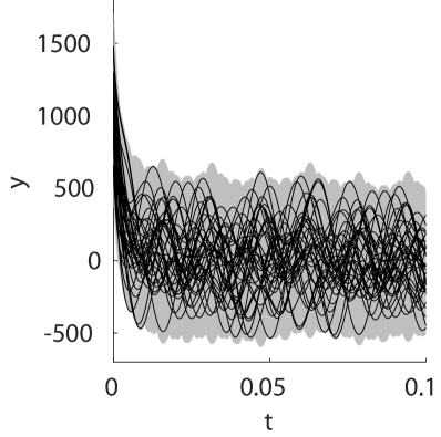
Refer to caption
(a) FOM model.
Refer to caption
(b) MNA-5 model.
Figure 4: Reachable set of outputs for selected benchmark models plotted over time. Black lines show random simulations, the gray area shows the reachable set.
Refer to captionRefer to captionRefer to captionRefer to captionRefer to captionRefer to captionRefer to captionRefer to captionRefer to captionRefer to captionRefer to captionRefer to caption
Figure 5: Two-dimensional projections of reachable sets for selected projections of the bridge model. Black lines show random simulations, the gray area shows the reachable set.

Verification

While the focus of this work is on reachability analysis, we also briefly demonstrate a possible verification of the bridge for which we check whether all states stay within certain axis-aligned bounds. Since the bounds consist of 25040=1008025040100802\cdot 5040=10080 values, we will only provide them within CORA. In the example, the reachable set respects the given bounds; checking the bounds for all time interval takes around 202020 s, which is small compared to 383538353835 s for the reachability analysis.

Discussion

Overall, the computational benefits of the Krylov methods typically improve with the size of the model as shown in Tab. II. When only the output is of importance, the Krylov method is particularly efficient since one can directly include the output matrix C𝐶C in the Krylov method by using the orthonormal basis V(v):=CV(v)assign𝑉𝑣𝐶𝑉𝑣V(v):=CV(v) as discussed in Sec. V-A (see also [29]). This avoids computing the reachable set of all states followed by projecting the result onto the outputs as required by standard methods. For the FOM model and the bridge model, the Krylov method is around 100 times faster, while the improvements for the MNA models are also substantial—only the small MNA-1 model shows similar computation times for both models.

In general, the computation times of the Kylov method are less predictable compared to the standard approach given the dimension of the system. While the computation times of the standard approach are typically monotonically increasing with the system dimension, the Krylov methods sometimes provides faster results for larger systems.

VII Conclusions

We have presented the first work for computing the over-approximative reachable set of linear systems in the Krylov subspace for arbitrarily-varying, bounded inputs. Unlike most other work on applying reduction techniques for reachability analysis, which compute an output abstraction, we perform a state abstraction and can fully reconstruct the complete reachable sets. When using output abstractions, only the reachable outputs can be over-approximated—if those output-abstraction techniques would be used to reconstruct the whole reachable set, no reduction would be achieved. Due to the strict consideration of error bounds, our approach can be used for formal verification and other formal techniques, such as computation of invariance sets, computation of the region of attraction, optimization of constrained systems with uncertainties, set-based observers, and conformance checking. In our numerical example we have seen a speed up of two orders of magnitude although the approximation was accurate up to floating point precision.

Acknowledgment

This work was partly supported by the German Research Foundation (DFG) under grant number AL 1185/5-1.

Appendix A Proof of Theorem IV.2

Proof.

We first compute an over-approximative reachable set resulting from inputs when assuming constant inputs for time intervals [t^k1,t^k[[\hat{t}_{k-1},\hat{t}_{k}[, where 0=t^0<t^1<<t^l1<t^l=δ0subscript^𝑡0subscript^𝑡1subscript^𝑡𝑙1subscript^𝑡𝑙𝛿0=\hat{t}_{0}<\hat{t}_{1}<\ldots<\hat{t}_{l-1}<\hat{t}_{l}=\delta, of equal duration ρ=t^kt^k1𝜌subscript^𝑡𝑘subscript^𝑡𝑘1\rho=\hat{t}_{k}-\hat{t}_{k-1}, so that

u(t)={u(0)for t[0,t^1[u(t^1)for t[t^1,t^2[u(t^l1)for t[t^l1,δ].u(t)=\begin{cases}u(0)&\text{for }t\in[0,\hat{t}_{1}[\\ u(\hat{t}_{1})&\text{for }t\in[\hat{t}_{1},\hat{t}_{2}[\\ \vdots&\\ u(\hat{t}_{l-1})&\text{for }t\in[\hat{t}_{l-1},\delta].\end{cases}

In a second step, we let ρ0𝜌0\rho\to 0 to obtain an over-approximation for arbitrarily varying inputs. The solution of piecewise constant inputs is obtained from

x𝚙,𝚙𝚠(δ)=0t1eA(δt)𝑑tu(0)+t1t2eA(δt)𝑑tu(t1)++tl1δeA(δt)𝑑tu(tl1).subscript𝑥𝚙𝚙𝚠𝛿superscriptsubscript0subscript𝑡1superscript𝑒𝐴𝛿𝑡differential-d𝑡𝑢0superscriptsubscriptsubscript𝑡1subscript𝑡2superscript𝑒𝐴𝛿𝑡differential-d𝑡𝑢subscript𝑡1superscriptsubscriptsubscript𝑡𝑙1𝛿superscript𝑒𝐴𝛿𝑡differential-d𝑡𝑢subscript𝑡𝑙1\begin{split}x_{\mathtt{p,pw}}(\delta)=&\int_{0}^{t_{1}}e^{A(\delta-t)}dt\,u(0)+\int_{t_{1}}^{t_{2}}e^{A(\delta-t)}dt\,u(t_{1})\\ &+\ldots+\int_{t_{l-1}}^{\delta}e^{A(\delta-t)}dt\,u(t_{l-1}).\end{split}

When the set of inputs is uncertain within 𝒰𝒰\mathcal{U}, we obtain

^p,l(δ)=0t1eA(δt)𝑑t𝒰tl1δeA(δt)𝑑t𝒰.subscript^𝑝𝑙𝛿direct-sumsuperscriptsubscript0subscript𝑡1superscript𝑒𝐴𝛿𝑡differential-d𝑡𝒰superscriptsubscriptsubscript𝑡𝑙1𝛿superscript𝑒𝐴𝛿𝑡differential-d𝑡𝒰\begin{split}\hat{\mathcal{R}}_{p,l}(\delta)=&\int_{0}^{t_{1}}e^{A(\delta-t)}\,dt\,\mathcal{U}\oplus\ldots\oplus\int_{t_{l-1}}^{\delta}e^{A(\delta-t)}\,dt\,\mathcal{U}.\end{split} (25)

In order to obtain not only an approximation, but an over-approximation, the solution for a time interval [tk1,tk[[t_{k-1},t_{k}[ is further abstracted. From Corrollary IV.1 we have that

^p([t0,te]):=t0teeA(δt)𝚍t𝒰P{V~(u)(eH~(u)(δt0)eH~(u)(δte))|u𝒰}e1[𝟏,𝟏]n{ϵ~norm(u)|u𝒰}(tet0).assignsubscript^𝑝subscript𝑡0subscript𝑡𝑒superscriptsubscriptsubscript𝑡0subscript𝑡𝑒superscript𝑒𝐴𝛿𝑡differential-d𝑡𝒰direct-sum𝑃conditional-set~𝑉𝑢superscript𝑒~𝐻𝑢𝛿subscript𝑡0superscript𝑒~𝐻𝑢𝛿subscript𝑡𝑒𝑢𝒰subscript𝑒1superscript11𝑛conditional-setsubscript~italic-ϵnorm𝑢𝑢𝒰subscript𝑡𝑒subscript𝑡0\begin{split}&\hat{\mathcal{R}}_{p}([t_{0},t_{e}]):=\int_{t_{0}}^{t_{e}}e^{A(\delta-t)}\mathtt{d}t\,\mathcal{U}\\ \subseteq&P\Big{\{}\tilde{V}(u)\big{(}e^{\tilde{H}(u)\,(\delta-t_{0})}-e^{\tilde{H}(u)\,(\delta-t_{e})}\big{)}\Big{|}u\in\mathcal{U}\Big{\}}e_{1}\\ &\oplus\mathbf{[-1,1]}^{n}\Big{\{}\tilde{\epsilon}_{\textrm{norm}}(u)\Big{|}u\in\mathcal{U}\Big{\}}(t_{e}-t_{0}).\end{split}

The above over-approximation is rewritten using a finite Taylor series (see (14)):

^p([t0,te])P{V~(u)(I+H~1(u)1!(δt0)1++H~η(u)η!(δt0)η+E~(δt0,u)(I+H~1(u)1!(δte)1++H~η(u)η!(δte)η+E~(δte,u)))|u𝒰,E~(t,u)~(t,u)}e1[𝟏,𝟏]n{ϵ~norm(u)|u𝒰}(tet0)=P{V~(u)H~1(u)1![(δt0)1(δte)1]++V~(u)H~η(u)η![(δt0)η(δte)η]+E~(δt0,u)E~(δte,u)|u𝒰,E~(t,u)~(t,u)}e1[𝟏,𝟏]n{ϵ~norm(u)|u𝒰}(tet0).subscript^𝑝subscript𝑡0subscript𝑡𝑒direct-sum𝑃conditional-set~𝑉𝑢𝐼superscript~𝐻1𝑢1superscript𝛿subscript𝑡01superscript~𝐻𝜂𝑢𝜂superscript𝛿subscript𝑡0𝜂~𝐸𝛿subscript𝑡0𝑢𝐼superscript~𝐻1𝑢1superscript𝛿subscript𝑡𝑒1superscript~𝐻𝜂𝑢𝜂superscript𝛿subscript𝑡𝑒𝜂~𝐸𝛿subscript𝑡𝑒𝑢formulae-sequence𝑢𝒰~𝐸𝑡𝑢~𝑡𝑢subscript𝑒1superscript11𝑛conditional-setsubscript~italic-ϵnorm𝑢𝑢𝒰subscript𝑡𝑒subscript𝑡0direct-sum𝑃conditional-set~𝑉𝑢superscript~𝐻1𝑢1delimited-[]superscript𝛿subscript𝑡01superscript𝛿subscript𝑡𝑒1~𝑉𝑢superscript~𝐻𝜂𝑢𝜂delimited-[]superscript𝛿subscript𝑡0𝜂superscript𝛿subscript𝑡𝑒𝜂~𝐸𝛿subscript𝑡0𝑢~𝐸𝛿subscript𝑡𝑒𝑢formulae-sequence𝑢𝒰~𝐸𝑡𝑢~𝑡𝑢subscript𝑒1superscript11𝑛conditional-setsubscript~italic-ϵnorm𝑢𝑢𝒰subscript𝑡𝑒subscript𝑡0\begin{split}&\hat{\mathcal{R}}_{p}([t_{0},t_{e}])\subseteq P\Big{\{}\tilde{V}(u)\Big{(}I+\frac{\tilde{H}^{1}(u)}{1!}(\delta-t_{0})^{1}+\ldots\\ &+\frac{\tilde{H}^{\eta}(u)}{\eta!}(\delta-t_{0})^{\eta}+\tilde{E}(\delta-t_{0},u)-\Big{(}I+\frac{\tilde{H}^{1}(u)}{1!}(\delta-t_{e})^{1}\\ &+\ldots+\frac{\tilde{H}^{\eta}(u)}{\eta!}(\delta-t_{e})^{\eta}+\tilde{E}(\delta-t_{e},u)\Big{)}\Big{)}\Big{|}u\in\mathcal{U},\\ &\tilde{E}(t,u)\in\tilde{\mathcal{E}}(t,u)\Big{\}}e_{1}\oplus\mathbf{[-1,1]}^{n}\Big{\{}\tilde{\epsilon}_{\textrm{norm}}(u)\Big{|}u\in\mathcal{U}\Big{\}}(t_{e}-t_{0})\\ =&P\Big{\{}\tilde{V}(u)\frac{\tilde{H}^{1}(u)}{1!}[(\delta-t_{0})^{1}-(\delta-t_{e})^{1}]+\ldots\\ &+\tilde{V}(u)\frac{\tilde{H}^{\eta}(u)}{\eta!}[(\delta-t_{0})^{\eta}-(\delta-t_{e})^{\eta}]\\ &+\tilde{E}(\delta-t_{0},u)-\tilde{E}(\delta-t_{e},u)\Big{|}u\in\mathcal{U},\\ &\tilde{E}(t,u)\in\tilde{\mathcal{E}}(t,u)\Big{\}}e_{1}\oplus\mathbf{[-1,1]}^{n}\Big{\{}\tilde{\epsilon}_{\textrm{norm}}(u)\Big{|}u\in\mathcal{U}\Big{\}}(t_{e}-t_{0}).\end{split}

Finally, the uncertainty of the input is moved inwards, which results in a further over-approximation:

^p([t0,te])P({V~(u)H~1(u)1!|u𝒰}[(δt0)1(δte)1]{V~(u)H~η(u)η!|u𝒰}[(δt0)η(δte)η]{E~(δt0,u)E~(δte,u)|u𝒰,E~(t,u)~(t,u)})e1[𝟏,𝟏]n{ϵ~norm(u)|u𝒰}(tet0).subscript^𝑝subscript𝑡0subscript𝑡𝑒direct-sum𝑃direct-sumconditional-set~𝑉𝑢superscript~𝐻1𝑢1𝑢𝒰delimited-[]superscript𝛿subscript𝑡01superscript𝛿subscript𝑡𝑒1conditional-set~𝑉𝑢superscript~𝐻𝜂𝑢𝜂𝑢𝒰delimited-[]superscript𝛿subscript𝑡0𝜂superscript𝛿subscript𝑡𝑒𝜂conditional-set~𝐸𝛿subscript𝑡0𝑢~𝐸𝛿subscript𝑡𝑒𝑢formulae-sequence𝑢𝒰~𝐸𝑡𝑢~𝑡𝑢subscript𝑒1superscript11𝑛conditional-setsubscript~italic-ϵnorm𝑢𝑢𝒰subscript𝑡𝑒subscript𝑡0\begin{split}&\hat{\mathcal{R}}_{p}([t_{0},t_{e}])\subseteq P\bigg{(}\\ &\Big{\{}\tilde{V}(u)\frac{\tilde{H}^{1}(u)}{1!}\Big{|}u\in\mathcal{U}\Big{\}}[(\delta-t_{0})^{1}-(\delta-t_{e})^{1}]\oplus\ldots\\ \oplus&\Big{\{}\tilde{V}(u)\frac{\tilde{H}^{\eta}(u)}{\eta!}\Big{|}u\in\mathcal{U}\Big{\}}[(\delta-t_{0})^{\eta}-(\delta-t_{e})^{\eta}]\\ \oplus&\Big{\{}\tilde{E}(\delta-t_{0},u)-\tilde{E}(\delta-t_{e},u)\Big{|}u\in\mathcal{U},\tilde{E}(t,u)\in\tilde{\mathcal{E}}(t,u)\Big{\}}\\ &\bigg{)}e_{1}\oplus\mathbf{[-1,1]}^{n}\Big{\{}\tilde{\epsilon}_{\textrm{norm}}(u)\Big{|}u\in\mathcal{U}\Big{\}}(t_{e}-t_{0}).\end{split} (26)

After introducing

𝒟(j):={V~(u)H~j(u)j!|u𝒰},assignsuperscript𝒟𝑗conditional-set~𝑉𝑢superscript~𝐻𝑗𝑢𝑗𝑢𝒰\mathcal{D}^{(j)}:=\Big{\{}\tilde{V}(u)\frac{\tilde{H}^{j}(u)}{j!}\Big{|}u\in\mathcal{U}\Big{\}},

one can rewrite (26) as

^p([t0,te])=t0teeA(δt)𝚍t𝒰P(𝒟(1)[(δt0)1(δte)1]𝒟(η)[(δt0)η(δte)η]{E~(δt0,u)E~(δte,u)|u𝒰,E~(t,u)~(t,u)})e1[𝟏,𝟏]n{ϵ~norm(u)|u𝒰}(tet0).subscript^𝑝subscript𝑡0subscript𝑡𝑒superscriptsubscriptsubscript𝑡0subscript𝑡𝑒superscript𝑒𝐴𝛿𝑡differential-d𝑡𝒰direct-sum𝑃direct-sumsuperscript𝒟1delimited-[]superscript𝛿subscript𝑡01superscript𝛿subscript𝑡𝑒1superscript𝒟𝜂delimited-[]superscript𝛿subscript𝑡0𝜂superscript𝛿subscript𝑡𝑒𝜂conditional-set~𝐸𝛿subscript𝑡0𝑢~𝐸𝛿subscript𝑡𝑒𝑢formulae-sequence𝑢𝒰~𝐸𝑡𝑢~𝑡𝑢subscript𝑒1superscript11𝑛conditional-setsubscript~italic-ϵnorm𝑢𝑢𝒰subscript𝑡𝑒subscript𝑡0\begin{split}&\hat{\mathcal{R}}_{p}([t_{0},t_{e}])=\int_{t_{0}}^{t_{e}}e^{A(\delta-t)}\mathtt{d}t\,\mathcal{U}\\ \subseteq&P\bigg{(}\mathcal{D}^{(1)}[(\delta-t_{0})^{1}-(\delta-t_{e})^{1}]\oplus\ldots\\ &\oplus\mathcal{D}^{(\eta)}[(\delta-t_{0})^{\eta}-(\delta-t_{e})^{\eta}]\\ &\oplus\Big{\{}\tilde{E}(\delta-t_{0},u)-\tilde{E}(\delta-t_{e},u)\Big{|}u\in\mathcal{U},\tilde{E}(t,u)\in\tilde{\mathcal{E}}(t,u)\Big{\}}\\ &\bigg{)}e_{1}\oplus\mathbf{[-1,1]}^{n}\Big{\{}\tilde{\epsilon}_{\textrm{norm}}(u)\Big{|}u\in\mathcal{U}\Big{\}}(t_{e}-t_{0}).\end{split} (27)

By repeatedly inserting (27) into (25), rearranging time intervals (δtk)=tlk𝛿subscript𝑡𝑘subscript𝑡𝑙𝑘(\delta-t_{k})=t_{l-k}, and using E~(t,u)~(t,u)=[W~(t,u),W~(t,u)]~𝐸𝑡𝑢~𝑡𝑢~𝑊𝑡𝑢~𝑊𝑡𝑢\tilde{E}(t,u)\in\tilde{\mathcal{E}}(t,u)=[-\tilde{W}(t,u),\tilde{W}(t,u)], where W~(t,u)=i=η+1tii!|H~(u)|i~𝑊𝑡𝑢superscriptsubscript𝑖𝜂1superscript𝑡𝑖𝑖superscript~𝐻𝑢𝑖\tilde{W}(t,u)=\sum_{i=\eta+1}^{\infty}\frac{t^{i}}{i!}|\tilde{H}(u)|^{i} from (15), we obtain

^p,l(δ)=P((𝒟(1)(tltl1)𝒟(η)(tlηtl1η)(𝒟(1)(tl1tl2)𝒟(η)(tl1ηtl2η)(𝒟(1)(t1t0)𝒟(η)(t1ηt0η){i=η+1tlitl1ii![|H~(u)|i,|H~(u)|i]i=η+1tl1itl2ii![|H~(u)|i,|H~(u)|i]i=η+1t1it0ii![|H~(u)|i,|H~(u)|i]|u𝒰})e1[𝟏,𝟏]n{ϵ~norm(u)|u𝒰}(tltl1)[𝟏,𝟏]n{ϵ~norm(u)|u𝒰}(tl1tl2)[𝟏,𝟏]n{ϵ~norm(u)|u𝒰}(t1t0).\begin{split}\hat{\mathcal{R}}_{p,l}(\delta)&=P\bigg{(}\\ &\begin{array}[]{rllll}&(\mathcal{D}^{(1)}(t_{l}-t_{l-1})&\oplus\ldots&\oplus\mathcal{D}^{(\eta)}(t_{l}^{\eta}-t_{l-1}^{\eta})\\ \oplus&(\mathcal{D}^{(1)}(t_{l-1}-t_{l-2})&\oplus\ldots&\oplus\mathcal{D}^{(\eta)}(t_{l-1}^{\eta}-t_{l-2}^{\eta})\\ \oplus&\ldots\\ \oplus&\underbrace{(\mathcal{D}^{(1)}(t_{1}-t_{0})}_{\bigoplus}&\oplus\ldots&\oplus\underbrace{\mathcal{D}^{(\eta)}(t_{1}^{\eta}-t_{0}^{\eta})}_{\bigoplus}\end{array}\\ &\begin{array}[]{rllll}\oplus\Big{\{}&\bigoplus_{i=\eta+1}^{\infty}\frac{t_{l}^{i}-t_{l-1}^{i}}{i!}\big{[}-|\tilde{H}(u)|^{i},|\tilde{H}(u)|^{i}\big{]}\\ \oplus&\bigoplus_{i=\eta+1}^{\infty}\frac{t_{l-1}^{i}-t_{l-2}^{i}}{i!}\big{[}-|\tilde{H}(u)|^{i},|\tilde{H}(u)|^{i}\big{]}\\ \oplus&\ldots\\ \oplus&\underbrace{\textstyle\bigoplus_{i=\eta+1}^{\infty}\frac{t_{1}^{i}-t_{0}^{i}}{i!}\big{[}-|\tilde{H}(u)|^{i},|\tilde{H}(u)|^{i}\big{]}}_{\bigoplus}\\ \end{array}\\ &\Big{|}u\in\mathcal{U}\Big{\}}\bigg{)}e_{1}\\ &\begin{array}[]{rllll}\oplus&\mathbf{[-1,1]}^{n}\Big{\{}\tilde{\epsilon}_{\textrm{norm}}(u)\Big{|}u\in\mathcal{U}\Big{\}}(t_{l}-t_{l-1})\\ \oplus&\mathbf{[-1,1]}^{n}\Big{\{}\tilde{\epsilon}_{\textrm{norm}}(u)\Big{|}u\in\mathcal{U}\Big{\}}(t_{l-1}-t_{l-2})\\ \oplus&\ldots\\ \oplus&\mathbf{[-1,1]}^{n}\Big{\{}\tilde{\epsilon}_{\textrm{norm}}(u)\Big{|}u\in\mathcal{U}\Big{\}}\underbrace{(t_{1}-t_{0})}_{\sum}.\\ \end{array}\\ \end{split} (28)

The summation symbols indicate that the terms written in one column are summed up. Since the expressions tkjtk1jsuperscriptsubscript𝑡𝑘𝑗superscriptsubscript𝑡𝑘1𝑗t_{k}^{j}-t_{k-1}^{j} are positive scalars, the following statement can be used for the summation: For any two positive scalars a,b+𝑎𝑏superscripta,b\in\mathbb{R}^{+} and the convex set 𝒮𝒮\mathcal{S}, one can state that a𝒮b𝒮=(a+b)𝒮direct-sum𝑎𝒮𝑏𝒮𝑎𝑏𝒮a\mathcal{S}\oplus b\mathcal{S}=(a+b)\mathcal{S}. From this follows that

𝒟(j)(t1jt0j)𝒟(j)(t2jt1j)𝒟(j)(tljtl1j)=𝒟(j)(tljt0j)=𝒟(j)tlj=𝒟(j)δjdirect-sumsuperscript𝒟𝑗superscriptsubscript𝑡1𝑗superscriptsubscript𝑡0𝑗superscript𝒟𝑗superscriptsubscript𝑡2𝑗superscriptsubscript𝑡1𝑗superscript𝒟𝑗superscriptsubscript𝑡𝑙𝑗superscriptsubscript𝑡𝑙1𝑗superscript𝒟𝑗superscriptsubscript𝑡𝑙𝑗superscriptsubscript𝑡0𝑗superscript𝒟𝑗superscriptsubscript𝑡𝑙𝑗superscript𝒟𝑗superscript𝛿𝑗\begin{split}&\mathcal{D}^{(j)}(t_{1}^{j}-t_{0}^{j})\oplus\mathcal{D}^{(j)}(t_{2}^{j}-t_{1}^{j})\oplus\ldots\oplus\mathcal{D}^{(j)}(t_{l}^{j}-t_{l-1}^{j})\\ &=\mathcal{D}^{(j)}(t_{l}^{j}-t_{0}^{j})=\mathcal{D}^{(j)}t_{l}^{j}=\mathcal{D}^{(j)}\delta^{j}\end{split} (29)

and similarly for the Taylor remainder terms

i=η+1t1it0ii![|H~(u)|i,|H~(u)|i]i=η+1tlitl1ii![|H~(u)|i,|H~(u)|i]=i=η+1tlit0ii![|H~(u)|i,|H~(u)|i]=~(δ,u)direct-sumsuperscriptsubscriptdirect-sum𝑖𝜂1superscriptsubscript𝑡1𝑖superscriptsubscript𝑡0𝑖𝑖superscript~𝐻𝑢𝑖superscript~𝐻𝑢𝑖superscriptsubscriptdirect-sum𝑖𝜂1superscriptsubscript𝑡𝑙𝑖superscriptsubscript𝑡𝑙1𝑖𝑖superscript~𝐻𝑢𝑖superscript~𝐻𝑢𝑖superscriptsubscriptdirect-sum𝑖𝜂1superscriptsubscript𝑡𝑙𝑖superscriptsubscript𝑡0𝑖𝑖superscript~𝐻𝑢𝑖superscript~𝐻𝑢𝑖~𝛿𝑢\begin{split}&\bigoplus_{i=\eta+1}^{\infty}\frac{t_{1}^{i}-t_{0}^{i}}{i!}\big{[}-|\tilde{H}(u)|^{i},|\tilde{H}(u)|^{i}\big{]}\oplus\ldots\oplus\\ &\bigoplus_{i=\eta+1}^{\infty}\frac{t_{l}^{i}-t_{l-1}^{i}}{i!}\big{[}-|\tilde{H}(u)|^{i},|\tilde{H}(u)|^{i}\big{]}\\ &=\bigoplus_{i=\eta+1}^{\infty}\frac{t_{l}^{i}-t_{0}^{i}}{i!}\big{[}-|\tilde{H}(u)|^{i},|\tilde{H}(u)|^{i}\big{]}=\tilde{\mathcal{E}}(\delta,u)\end{split} (30)

and the Krylov error terms

[𝟏,𝟏]n{ϵ~norm(u)|u𝒰}(t1t0)[𝟏,𝟏]n{ϵ~norm(u)|u𝒰}(tltl1)=[𝟏,𝟏]n{ϵ~norm(u)|u𝒰}δ.direct-sumsuperscript11𝑛conditional-setsubscript~italic-ϵnorm𝑢𝑢𝒰subscript𝑡1subscript𝑡0superscript11𝑛conditional-setsubscript~italic-ϵnorm𝑢𝑢𝒰subscript𝑡𝑙subscript𝑡𝑙1superscript11𝑛conditional-setsubscript~italic-ϵnorm𝑢𝑢𝒰𝛿\begin{split}&\mathbf{[-1,1]}^{n}\Big{\{}\tilde{\epsilon}_{\textrm{norm}}(u)\Big{|}u\in\mathcal{U}\Big{\}}(t_{1}-t_{0})\oplus\ldots\oplus\\ &\mathbf{[-1,1]}^{n}\Big{\{}\tilde{\epsilon}_{\textrm{norm}}(u)\Big{|}u\in\mathcal{U}\Big{\}}(t_{l}-t_{l-1})\\ &=\mathbf{[-1,1]}^{n}\Big{\{}\tilde{\epsilon}_{\textrm{norm}}(u)\Big{|}u\in\mathcal{U}\Big{\}}\delta.\end{split} (31)

Inserting (29) - (31) into (28) yields

^p,l(δ)=P(𝒟(1)δ𝒟(η)δη{~(δ,u)|u𝒰})e1[𝟏,𝟏]n{ϵ~norm(u)|u𝒰}δ.subscript^𝑝𝑙𝛿direct-sum𝑃direct-sumsuperscript𝒟1𝛿superscript𝒟𝜂superscript𝛿𝜂conditional-set~𝛿𝑢𝑢𝒰subscript𝑒1superscript11𝑛conditional-setsubscript~italic-ϵnorm𝑢𝑢𝒰𝛿\begin{split}\hat{\mathcal{R}}_{p,l}(\delta)=&P\bigg{(}\mathcal{D}^{(1)}\delta\oplus\ldots\oplus\mathcal{D}^{(\eta)}\delta^{\eta}\\ \oplus&\Big{\{}\tilde{\mathcal{E}}(\delta,u)\Big{|}u\in\mathcal{U}\Big{\}}\bigg{)}e_{1}\\ \oplus&\mathbf{[-1,1]}^{n}\Big{\{}\tilde{\epsilon}_{\textrm{norm}}(u)\Big{|}u\in\mathcal{U}\Big{\}}\delta.\end{split}

Since the above result is independent of the number of intermediate time steps l𝑙l, we can choose l𝑙l\to\infty, meaning that

liml^p,l(δ)=p(δ).subscript𝑙subscript^𝑝𝑙𝛿subscript𝑝𝛿\begin{split}\lim_{l\to\infty}\hat{\mathcal{R}}_{p,l}(\delta)=\mathcal{R}_{p}(\delta).\end{split}

Appendix B Error Bound for the Approximation of Matrix Exponentials

In this work, we use the a-posteriori bound from [58, Eq. 4.1]. A method for efficient computation of this bound is presented in the subsequent proposition.

Proposition B.1.

The error bound

t[0,tf]:eCtvvVeHte1vϵ¯normt:for-all𝑡0subscript𝑡𝑓normlimit-fromsuperscript𝑒𝐶𝑡𝑣𝑣norm𝑉superscript𝑒𝐻𝑡subscript𝑒1norm𝑣subscript¯italic-ϵnorm𝑡\forall t\in[0,t_{f}]:\big{\|}e^{Ct}v-\|v\|Ve^{Ht}e_{1}\big{\|}\leq\|v\|\overline{\epsilon}_{\textrm{norm}}\,t

in (3) holds for

ϵ¯norm=hξ+1,ξω¯φ¯,φ¯={eν(C)tf1ν(C)tf, for ν(C)>0,1, otherwise.ω¯=maxk{1,,tf/δ}(ωk),ωk=eξTeHtkeH[0,δ]e1,H[0,δ]={0.5Hδ+β0.5Hδ|β[1,1]},formulae-sequenceformulae-sequencesubscript¯italic-ϵnormsubscript𝜉1𝜉¯𝜔¯𝜑¯𝜑casessuperscript𝑒𝜈𝐶subscript𝑡𝑓1𝜈𝐶subscript𝑡𝑓, for 𝜈𝐶01, otherwise¯𝜔subscript𝑘1subscript𝑡𝑓𝛿subscript𝜔𝑘formulae-sequencesubscript𝜔𝑘superscriptsubscript𝑒𝜉𝑇superscript𝑒𝐻subscript𝑡𝑘superscript𝑒𝐻0𝛿subscript𝑒1𝐻0𝛿conditional-set0.5𝐻𝛿𝛽0.5𝐻𝛿𝛽11\begin{split}\overline{\epsilon}_{\textrm{norm}}=&h_{\xi+1,\xi}\,\overline{\omega}\,\overline{\varphi},\\ \overline{\varphi}=&\begin{cases}\frac{e^{\nu(C)t_{f}}-1}{\nu(C)t_{f}}&\text{, for }\nu(C)>0,\\ 1&\text{, otherwise}.\end{cases}\\ \overline{\omega}=&\max_{k\in\{1,\ldots,\lceil t_{f}/\delta\rceil\}}(\omega_{k}),\\ \omega_{k}=&e_{\xi}^{T}e^{Ht_{k}}e^{H[0,\delta]}e_{1},\\ H[0,\delta]=&\{0.5H\delta+\beta 0.5H\delta|\beta\in[-1,1]\},\end{split}

where H[0,δ]𝐻0𝛿H[0,\delta] can be represented as a matrix zonotope, i.e., a zonotope whose center and generators are replaced by matrices; the exponential of a matrix zonotope eH[0,δ]superscript𝑒𝐻0𝛿e^{H[0,\delta]} can be computed as presented in [73]. Further, ν(C):=λmax(0.5(C+C))assign𝜈𝐶subscript𝜆𝑚𝑎𝑥0.5𝐶superscript𝐶\nu(C):=\lambda_{max}(0.5(C+C^{*})) returns the largest eigenvalue and Csuperscript𝐶C^{*} is the conjugate transpose of C𝐶C. Please note that the computation of ν(C)𝜈𝐶\nu(C) can be done efficiently since 0.5(C+C)0.5𝐶superscript𝐶0.5(C+C^{*}) is a real, sparse, symmetric matrix for which efficient eigenvalue computations [74, 75] exist. Results can be obtained up to machine precision [76] and error bounds are derived in [77, 78]. Finally, eξsubscript𝑒𝜉e_{\xi} is the unit vector whose ξthsuperscript𝜉th\xi^{\text{th}} value is one and the values of hξ+1,ξsubscript𝜉1𝜉h_{\xi+1,\xi} and H𝐻H are taken from Alg. 1.

Proof.

The a-posteriori bound from [58, Eq. 4.1] is

eCtfvvVeHtfe1vhξ+1,ξmaxt[0,tf]|eξTeHte1|eν(C)tf1ν(C).delimited-∥∥limit-fromsuperscript𝑒𝐶subscript𝑡𝑓𝑣𝑣delimited-∥∥𝑉superscript𝑒𝐻subscript𝑡𝑓subscript𝑒1delimited-∥∥𝑣subscript𝜉1𝜉subscript𝑡0subscript𝑡𝑓superscriptsubscript𝑒𝜉𝑇superscript𝑒𝐻𝑡subscript𝑒1superscript𝑒𝜈𝐶subscript𝑡𝑓1𝜈𝐶\begin{split}&\big{\|}e^{Ct_{f}}v-\|v\|Ve^{Ht_{f}}e_{1}\big{\|}\\ \leq&\|v\|h_{\xi+1,\xi}\max_{t\in[0,t_{f}]}|e_{\xi}^{T}e^{Ht}e_{1}|\frac{e^{\nu(C)t_{f}}-1}{\nu(C)}.\end{split} (32)

Please note that some signs are changed compared to [58, Eq. 4.1] since in that work, the system is specified as x˙=eCt˙𝑥superscript𝑒𝐶𝑡\dot{x}=e^{-Ct} instead of x˙=eCt˙𝑥superscript𝑒𝐶𝑡\dot{x}=e^{Ct}.

Error bound is linear in time

The error bound can be enclosed by a function that is linear in time. From (32) we can derive the following bound:

t[0,tf]:eCtvvVeHte1vhξ+1,ξmaxt^[0,t](|eξTeHt^e1|)eν(C)t1ν(C)=tvhξ+1,ξmaxt^[0,t](|eξTeHt^e1|)eν(C)t1ν(C)ttvhξ+1,ξmaxt^[0,tf](|eξTeHt^e1|)maxt^[0,tf](eν(C)t^1ν(C)t^=:φ(t^)):for-all𝑡0subscript𝑡𝑓delimited-∥∥limit-fromsuperscript𝑒𝐶𝑡𝑣𝑣delimited-∥∥𝑉superscript𝑒𝐻𝑡subscript𝑒1delimited-∥∥𝑣subscript𝜉1𝜉subscript^𝑡0𝑡superscriptsubscript𝑒𝜉𝑇superscript𝑒𝐻^𝑡subscript𝑒1superscript𝑒𝜈𝐶𝑡1𝜈𝐶𝑡delimited-∥∥𝑣subscript𝜉1𝜉subscript^𝑡0𝑡superscriptsubscript𝑒𝜉𝑇superscript𝑒𝐻^𝑡subscript𝑒1superscript𝑒𝜈𝐶𝑡1𝜈𝐶𝑡𝑡delimited-∥∥𝑣subscript𝜉1𝜉subscript^𝑡0subscript𝑡𝑓superscriptsubscript𝑒𝜉𝑇superscript𝑒𝐻^𝑡subscript𝑒1subscript^𝑡0subscript𝑡𝑓subscriptsuperscript𝑒𝜈𝐶^𝑡1𝜈𝐶^𝑡:absent𝜑^𝑡\begin{split}&\forall t\in[0,t_{f}]:\big{\|}e^{Ct}v-\|v\|Ve^{Ht}e_{1}\big{\|}\\ \leq&\|v\|h_{\xi+1,\xi}\max_{\hat{t}\in[0,t]}\Big{(}|e_{\xi}^{T}e^{H\hat{t}}e_{1}|\Big{)}\frac{e^{\nu(C)t}-1}{\nu(C)}\\ =&t\,\|v\|h_{\xi+1,\xi}\max_{\hat{t}\in[0,t]}\Big{(}|e_{\xi}^{T}e^{H\hat{t}}e_{1}|\Big{)}\frac{e^{\nu(C)t}-1}{\nu(C)t}\\ \leq&t\,\|v\|h_{\xi+1,\xi}\max_{\hat{t}\in[0,t_{f}]}\Big{(}|e_{\xi}^{T}e^{H\hat{t}}e_{1}|\Big{)}\max_{\hat{t}\in[0,t_{f}]}\bigg{(}\underbrace{\frac{e^{\nu(C)\hat{t}}-1}{\nu(C)\hat{t}}}_{=:\varphi(\hat{t})}\bigg{)}\\ \end{split} (33)

Depending on ν(C)𝜈𝐶\nu(C), the function φ(t)𝜑𝑡\varphi(t) is monotonically increasing or decreasing. To show this, we insert the Taylor series eν(C)t=i=0(ν(C)t)nn!superscript𝑒𝜈𝐶𝑡superscriptsubscript𝑖0superscript𝜈𝐶𝑡𝑛𝑛e^{\nu(C)t}=\sum_{i=0}^{\infty}\frac{(\nu(C)t)^{n}}{n!} in the derivative

φ˙(t)=ν(C)teν(C)teν(C)t+1ν(C)t2˙𝜑𝑡𝜈𝐶𝑡superscript𝑒𝜈𝐶𝑡superscript𝑒𝜈𝐶𝑡1𝜈𝐶superscript𝑡2\dot{\varphi}(t)=\frac{\nu(C)te^{\nu(C)t}-e^{\nu(C)t}+1}{\nu(C)t^{2}}

so that we obtain

φ˙(t)=ν(C)t(1+ν(C)t+(ν(C)t)22!+)ν(C)t2(1+ν(C)t+(ν(C)t)22!+)1ν(C)t2=(ν(C)t)2+(ν(C)t)32!+)(ν(C)t)22!(ν(C)t)33!ν(C)t2=i=0(1(n+1)!1(n+2)!)(ν(C)t)n+2ν(C)t2=ν(C)i=0(1n+11(n+2)(n+1))(ν(C)t)nn!ν(C)i=0]0,0.5](ν(C)t)nn!=ν(C)]0,0.5]i=0(ν(C)t)nn!=ν(C)]0,0.5]e(ν(C)t)>0.\begin{split}\dot{\varphi}(t)=&\frac{\nu(C)t(1+\nu(C)t+\frac{(\nu(C)t)^{2}}{2!}+\ldots)}{\nu(C)t^{2}}\\ -&\frac{(1+\nu(C)t+\frac{(\nu(C)t)^{2}}{2!}+\ldots)-1}{\nu(C)t^{2}}\\ =&\frac{(\nu(C)t)^{2}+\frac{(\nu(C)t)^{3}}{2!}+\ldots)-\frac{(\nu(C)t)^{2}}{2!}-\frac{(\nu(C)t)^{3}}{3!}-\ldots}{\nu(C)t^{2}}\\ =&\sum_{i=0}^{\infty}\bigg{(}\frac{1}{(n+1)!}-\frac{1}{(n+2)!}\bigg{)}\frac{(\nu(C)t)^{n+2}}{\nu(C)t^{2}}\\ =&\nu(C)\sum_{i=0}^{\infty}\bigg{(}\frac{1}{n+1}-\frac{1}{(n+2)(n+1)}\bigg{)}\frac{(\nu(C)t)^{n}}{n!}\\ \in&\nu(C)\sum_{i=0}^{\infty}]0,0.5]\frac{(\nu(C)t)^{n}}{n!}\\ =&\nu(C)]0,0.5]\sum_{i=0}^{\infty}\frac{(\nu(C)t)^{n}}{n!}=\nu(C)\underbrace{]0,0.5]e^{(\nu(C)t)}}_{>0}.\end{split}

Thus, φ(t)𝜑𝑡\varphi(t) is monotonically increasing if ν(C)>0𝜈𝐶0\nu(C)>0, monotonically decreasing for ν(C)<0𝜈𝐶0\nu(C)<0, and constant for ν(C)=0𝜈𝐶0\nu(C)=0. As a consequence, the maximum is obtained at t=tf𝑡subscript𝑡𝑓t=t_{f} for ν(C)>0𝜈𝐶0\nu(C)>0 and at t=0𝑡0t=0 for ν(C)0𝜈𝐶0\nu(C)\leq 0. For the evaluation of t=0𝑡0t=0, we require the rule of L’Hôpital:

limt0eν(C)t1ν(C)t=limt0ν(C)eν(C)tν(C)=limt0eν(C)t=1.subscript𝑡0superscript𝑒𝜈𝐶𝑡1𝜈𝐶𝑡subscript𝑡0𝜈𝐶superscript𝑒𝜈𝐶𝑡𝜈𝐶subscript𝑡0superscript𝑒𝜈𝐶𝑡1\lim_{t\to 0}\frac{e^{\nu(C)t}-1}{\nu(C)t}=\lim_{t\to 0}\frac{\nu(C)e^{\nu(C)t}}{\nu(C)}=\lim_{t\to 0}e^{\nu(C)t}=1.

The maximum is then obtained by

φ¯=maxt^[0,tf]φ(t^)={eν(C)tf1ν(C)tf, for ν(C)>0,1, otherwise.¯𝜑subscript^𝑡0subscript𝑡𝑓𝜑^𝑡casessuperscript𝑒𝜈𝐶subscript𝑡𝑓1𝜈𝐶subscript𝑡𝑓, for 𝜈𝐶01, otherwise\overline{\varphi}=\max_{\hat{t}\in[0,t_{f}]}\varphi(\hat{t})=\begin{cases}\frac{e^{\nu(C)t_{f}}-1}{\nu(C)t_{f}}&\text{, for }\nu(C)>0,\\ 1&\text{, otherwise}.\end{cases} (34)

Computation of maxt^[0,tf]|eξTeHt^e1|subscript^𝑡0subscript𝑡𝑓superscriptsubscript𝑒𝜉𝑇superscript𝑒𝐻^𝑡subscript𝑒1\max_{\hat{t}\in[0,t_{f}]}|e_{\xi}^{T}e^{H\hat{t}}e_{1}|

To compute maxt^[0,tf]|eξTeHt^e1|subscript^𝑡0subscript𝑡𝑓superscriptsubscript𝑒𝜉𝑇superscript𝑒𝐻^𝑡subscript𝑒1\max_{\hat{t}\in[0,t_{f}]}|e_{\xi}^{T}e^{H\hat{t}}e_{1}|, we compute

eHτk=eHtkeH[0,δ]superscript𝑒𝐻subscript𝜏𝑘superscript𝑒𝐻subscript𝑡𝑘superscript𝑒𝐻0𝛿e^{H\tau_{k}}=e^{Ht_{k}}e^{H[0,\delta]}

as presented in [73, Eq. 4.10] using the matrix zonotope (see [73, Eq. 4.8])

H[0,δ]={0.5Hδ+β0.5Hδ|β[1,1]}.𝐻0𝛿conditional-set0.5𝐻𝛿𝛽0.5𝐻𝛿𝛽11H[0,\delta]=\{0.5H\delta+\beta 0.5H\delta|\beta\in[-1,1]\}.

Let us also introduce

ωk=eξTeHτke1.subscript𝜔𝑘superscriptsubscript𝑒𝜉𝑇superscript𝑒𝐻subscript𝜏𝑘subscript𝑒1\omega_{k}=e_{\xi}^{T}e^{H\tau_{k}}e_{1}.

Since ωksubscript𝜔𝑘\omega_{k} is one-dimensional, the result is the interval maxtτk(eξTeHte1)=sup(ωk)subscript𝑡subscript𝜏𝑘superscriptsubscript𝑒𝜉𝑇superscript𝑒𝐻𝑡subscript𝑒1supremumsubscript𝜔𝑘\max_{t\in\tau_{k}}(e_{\xi}^{T}e^{Ht}e_{1})=\sup(\omega_{k}). For the entire time horizon, the maximum is simply obtained as

ω¯=maxt[0,tf]|eξTeHte1|=maxk{1,,tf/δ}(ωk).¯𝜔subscript𝑡0subscript𝑡𝑓superscriptsubscript𝑒𝜉𝑇superscript𝑒𝐻𝑡subscript𝑒1subscript𝑘1subscript𝑡𝑓𝛿subscript𝜔𝑘\overline{\omega}=\max_{t\in[0,t_{f}]}|e_{\xi}^{T}e^{Ht}e_{1}|=\max_{k\in\{1,\ldots,\lceil t_{f}/\delta\rceil\}}(\omega_{k}). (35)

Final Result

using (35) and (34) in (33) results in the proposition:

t[0,tf]:eCtvvVeHte1tvhξ+1,ξω¯φ¯.:for-all𝑡0subscript𝑡𝑓delimited-∥∥limit-fromsuperscript𝑒𝐶𝑡𝑣𝑣delimited-∥∥𝑉superscript𝑒𝐻𝑡subscript𝑒1𝑡delimited-∥∥𝑣subscript𝜉1𝜉¯𝜔¯𝜑\begin{split}\forall t\in[0,t_{f}]:&\big{\|}e^{Ct}v-\|v\|Ve^{Ht}e_{1}\big{\|}\\ \leq&t\,\|v\|h_{\xi+1,\xi}\,\overline{\omega}\,\overline{\varphi}.\end{split}

As a short final remark, we would like to mention that we have used the MATLAB function eigseigs\mathrm{eigs} to obtain λmaxsubscript𝜆𝑚𝑎𝑥\lambda_{max}.

References

  • [1] A. Banerjee, K. K. Venkatasubramanian, T. Mukherjee, and S. K. S. Gupta, “Ensuring safety, security, and sustainability of mission-critical cyber-physical systems,” Proceedings of the IEEE, vol. 100, no. 1, pp. 283–299, 2012.
  • [2] E. Asarin, T. Dang, G. Frehse, A. Girard, C. Le Guernic, and O. Maler, “Recent progress in continuous and hybrid reachability analysis,” in Proc. of the IEEE Conference on Computer Aided Control Systems Design, 2006, pp. 1582–1587.
  • [3] I. Kolmanovsky and E. G. Gilbert, “Theory and computation of disturbance invariant sets for discrete-time linear systems,” Mathematical Problems in Engineering, vol. 4, pp. 317–367, 1998.
  • [4] F. Blanchini, “Set invariance in control,” Automatica, vol. 35, no. 11, pp. 1747 – 1767, 1999.
  • [5] A. El-Guindy, D. Han, and M. Althoff, “Estimating the region of attraction via forward reachable sets,” in Proc. of the American Control Conference, 2017, pp. 1263–1270.
  • [6] D. Limon, I. Alvarado, T. Alamo, and E. F.Camacho, “Robust tube-based MPC for tracking of constrained linear systems with additive disturbances,” Journal of Process Control, vol. 20, no. 3, pp. 248–260, 2010.
  • [7] B. Schürmann and M. Althoff, “Convex interpolation control with formal guarantees for disturbed and constrained nonlinear systems,” in Proc. of Hybrid Systems: Computation and Control, 2017, pp. 121–130.
  • [8] C. Combastel, “A state bounding observer for uncertain non-linear continuous-time systems based on zonotopes,” in Proc. of the 44th IEEE Conference on Decision and Control, and the European Control Conference, 2005, pp. 7228–7234.
  • [9] V. T. H. Le, C. Stoica, T. Alamo, E. F. Camacho, and D. Dumur, Zonotopes: From Guaranteed State-estimation to Control.   Wiley, 2013.
  • [10] H. Roehm, J. Oehlerking, M. Woehrle, and M. Althoff, “Reachset conformance testing of hybrid automata,” in Proc. of Hybrid Systems: Computation and Control, 2016, pp. 277–286.
  • [11] P. Falcone, M. Ali, and J. Sjöberg, “Predictive threat assessment via reachability analysis and set invariance theory,” IEEE Transactions on Intelligent Transportation Systems, vol. 12, no. 4, pp. 1352–1361, 2011.
  • [12] M. Althoff and J. M. Dolan, “Online verification of automated road vehicles using reachability analysis,” IEEE Transactions on Robotics, vol. 30, no. 4, pp. 903–918, 2014.
  • [13] H. Täubig, U. Frese, C. Hertzberg, C. Lüth, S. Mohr, E. Vorobev, and D. Walter, “Guaranteeing functional safety: design for provability and computer-aided verification,” Autonomous Robots, vol. 32, no. 3, pp. 303–331, 2012.
  • [14] A. Pereira and M. Althoff, “Overapproximative arm occupancy prediction for human-robot interaction built from archetypal movements,” in International Conference on Robotics and Automation, 2016, pp. 1394–1401.
  • [15] H. N. Villegas Pico and D. C. Aliprantis, “Voltage ride-through capability verification of wind turbines with fully-rated converters using reachability analysis,” IEEE Transactions on Energy Conversion, vol. 29, no. 2, pp. 392–405, 2014.
  • [16] A. El-Guindy, D. Han, and M. Althoff, “Formal analysis of drum-boiler units to maximize the load-following capabilities of power plants,” IEEE Transactions on Power Systems, vol. 31, no. 6, pp. 4691–4702, 2016.
  • [17] G. Frehse, B. H. Krogh, and R. A. Rutenbar, “Verifying analog oscillator circuits using forward/backward abstraction refinement,” in Proc. of Design, Automation and Test in Europe, 2006.
  • [18] M. Althoff, A. Rajhans, B. H. Krogh, S. Yaldiz, X. Li, and L. Pileggi, “Formal verification of phase-locked loops using reachability analysis and continuization,” Communications of the ACM, vol. 56, no. 10, pp. 97–104, 2013.
  • [19] T. Dang, “Vérification et synthèse des systèmes hybrides,” Ph.D. dissertation, Institut National Polytechnique de Grenoble, 2000.
  • [20] A. A. Kurzhanskiy and P. Varaiya, “Ellipsoidal techniques for reachability analysis of discrete-time linear systems,” IEEE Transactions on Automatic Control, vol. 52, no. 1, pp. 26–38, 2007.
  • [21] A. Chutinan and B. H. Krogh, “Computational techniques for hybrid system verification,” IEEE Transactions on Automatic Control, vol. 48, no. 1, pp. 64–75, 2003.
  • [22] A. Girard, “Reachability of uncertain linear systems using zonotopes,” in Hybrid Systems: Computation and Control, ser. LNCS 3414.   Springer, 2005, pp. 291–305.
  • [23] M. Althoff and B. H. Krogh, “Zonotope bundles for the efficient computation of reachable sets,” in Proc. of the 50th IEEE Conference on Decision and Control, 2011, pp. 6814–6821.
  • [24] A. Girard and C. Le Guernic, “Efficient reachability analysis for linear systems using support functions,” in Proc. of the 17th IFAC World Congress, 2008, pp. 8966–8971.
  • [25] I. M. Mitchell, A. M. Bayen, and C. J. Tomlin, “A time-dependent Hamilton–Jacobi formulation of reachable sets for continuous dynamic games,” IEEE Transactions on Automatic Control, vol. 50, pp. 947–957, 2005.
  • [26] M. Althoff and G. Frehse, “Combining zonotopes and support functions for efficient reachability analysis of linear systems,” in Proc. of the 55th IEEE Conference on Decision and Control, 2016, pp. 7439–7446.
  • [27] P. S. Duggirala and M. Viswanathan, “Parsimonious, simulation based verification of linear systems,” in Proc. of International Conference on Computer Aided Verification, 2016, pp. 477–494.
  • [28] S. Bak and P. S. Duggirala, “HyLAA: A tool for computing simulation-equivalent reachability for linear systems,” in Proc. of the 20th International Conference on Hybrid Systems: Computation and Control, 2017, pp. 173–178.
  • [29] S. Bak, H.-D. Tran, and T. T. Johnson. (2018) Numerical verification of affine systems with up to a billion dimensions. arXiv:1804.01583v2.
  • [30] S. Bak and P. S. Duggirala, “Simulation-equivalent reachability of large linear systems with inputs,” in Proc. of International Conference on Computer Aided Verification, 2017, pp. 401–420.
  • [31] S. Bogomolov, M. Forets, G. Frehse, F. Viry, A. Podelski, and C. Schilling, “Reach set approximation through decomposition with low-dimensional sets and high-dimensional matrices,” in Proc. of the 21st International Conference on Hybrid Systems: Computation and Control, 2018, pp. 41–50.
  • [32] G. Lafferriere, G. J. Pappas, and S. Yovine, “A new class of decidable hybrid systems,” in Hybrid Systems: Computation and Control, ser. LNCS 1569.   Springer, 1999, pp. 137–151.
  • [33] E. Asarin, T. Dang, and A. Girard, “Hybridization methods for the analysis of nonlinear systems,” Acta Informatica, vol. 43, pp. 451–476, 2007.
  • [34] M. Althoff, O. Stursberg, and M. Buss, “Reachability analysis of nonlinear systems with uncertain parameters using conservative linearization,” in Proc. of the 47th IEEE Conference on Decision and Control, 2008, pp. 4042–4048.
  • [35] T. Dang, O. Maler, and R. Testylier, “Accurate hybridization of nonlinear systems,” in Hybrid Systems: Computation and Control, 2010, pp. 11–19.
  • [36] C. Moler and C. V. Loan, “Nineteen dubious ways to compute the exponential of a matrix, twenty-five years later,” SIAM Review, vol. 45, no. 1, pp. 3–49, 2003.
  • [37] Y. Saad, Iterative Methods for Sparse Linear Systems.   Society for Industrial and Applied Mathematics, 2003.
  • [38] A. C. Antoulas, Approximation of Large-Scale Dynamical Systems.   Society for Industrial and Applied Mathematics, 2005.
  • [39] W. H. A. Schilders, H. A. van der Vorst, and J. Rommes, Model Order Reduction: Theory, Research Aspects and Applications.   Springer, 2008.
  • [40] Z. Han and B. Krogh, “Reachability analysis of hybrid control systems using reduced-order models,” in Proc. of the American Control Conference, 2004, pp. 1183–1189.
  • [41] G. Frehse, C. L. Guernic, A. Donzé, S. Cotton, R. Ray, O. Lebeltel, R. Ripado, A. Girard, T. Dang, and O. Maler, “SpaceEx: Scalable verification of hybrid systems,” in Proc. of the 23rd International Conference on Computer Aided Verification, ser. LNCS 6806.   Springer, 2011, pp. 379–395.
  • [42] X. Chen, E. Ábrahám, and S. Sankaranarayanan, “Flow*: An analyzer for non-linear hybrid systems,” in Proc. of Computer-Aided Verification, ser. LNCS 8044.   Springer, 2013, pp. 258–263.
  • [43] A. Gurung, A. Deka, E. Bartocci, S. Bogomolov, R. Grosu, and R. Ray, “Parallel reachability analysis for hybrid systems,” in Proc. of the ACM/IEEE International Conference on Formal Methods and Models for System Design, 2016, pp. 12–22.
  • [44] M. Althoff, “An introduction to CORA 2015,” in Proc. of the Workshop on Applied Verification for Continuous and Hybrid Systems, 2015, pp. 120–151.
  • [45] M. Althoff, S. Bak, D. Cattaruzza, X. Chen, G. Frehse, R. Ray, and S. Schupp, “ARCH-COMP17 category report: Continuous and hybrid systems with linear continuous dynamics,” in Proc. of the 4th International Workshop on Applied Verification for Continuous and Hybrid Systems, 2017, pp. 143–159.
  • [46] M. Althoff, S. Bak, X. Chen, C. Fan, M. Forets, G. Frehse, N. Kochdumper, Y. Li, S. Mitra, R. Ray, C. Schilling, and S. Schupp, “ARCH-COMP18 category report: Continuous and hybrid systems with linear continuous dynamics,” in Proc. of the 5th International Workshop on Applied Verification for Continuous and Hybrid Systems, 2018, pp. 23–52.
  • [47] Z. Han and B. H. Krogh, “Reachability analysis of large-scale affine systems using low-dimensional polytopes,” in Hybrid Systems: Computation and Control, ser. LNCS 3927.   Springer, 2006, pp. 287–301.
  • [48] H.-D. Tran, L. V. Nguyen, W. Xiang, and T. T. Johnson, “Order-reduction abstractions for safety verification of high-dimensional linear systems,” Discrete Event Dynamic Systems, vol. 27, no. 2, pp. 443–461, 2017.
  • [49] Y. Chou, X. Chen, and S. Sankaranarayanan, “A study of model-order reduction techniques for verification,” in Proc. of Numerical Software Verification, 2017, pp. 98–113.
  • [50] A. J. van der Schaft, “Equivalence of dynamical systems by bisimulation,” IEEE Transactions on Automatic Control, vol. 49, no. 12, pp. 2160–2172, 2004.
  • [51] A. Girard and G. J. Pappas, “Approximate bisimulation: A bridge between computer science and control theory,” European Journal of Control, vol. 17, no. 5-6, pp. 568–578, 2011.
  • [52] J. G. VanAntwerp and R. D. Braatz, “A tutorial on linear and bilinear matrix inequalities,” Journal of Process Control, vol. 10, pp. 363–385, 2000.
  • [53] A. Girard and G. J. Pappas, “Approximate bisimulation relations for constrained linear systems,” Automatica, vol. 43, pp. 1307–1317, 2007.
  • [54] M. Althoff, O. Stursberg, and M. Buss, “Computing reachable sets of hybrid systems using a combination of zonotopes and polytopes,” Nonlinear Analysis: Hybrid Systems, vol. 4, no. 2, pp. 233–249, 2010.
  • [55] Y. Saad, “Analysis of some Krylov subspace approximations to the matrix exponential operator,” SIAM Journal on Numerical Analysis, vol. 29, no. 1, pp. 209–228, 1992.
  • [56] M. Hochbruck and C. Lubich, “On Krylov subspace approximations to the matrix exponential operator,” SIAM Journal on Numerical Analysis, vol. 34, no. 5, pp. 1911–1925, 1997.
  • [57] R. B. Sidje, “Expokit: A software package for computing matrix exponentials,” ACM Transactions on Mathematical Software, vol. 24, no. 1, pp. 130–156, 1998.
  • [58] Z. Jia and H. Lv, “A posteriori error estimates of Krylov subspace approximations to matrix functions,” Numerical Algorithms, vol. 69, no. 1, pp. 1–28, 2015.
  • [59] H. Wang and Q. Ye, “Error bounds for the Krylov subspace methods for computations of matrix exponentials,” SIAM Journal on Matrix Analysis and Applications, vol. 38, no. 1, pp. 155–187, 2017.
  • [60] W. Kühn, “Rigorously computed orbits of dynamical systems without the wrapping effect,” Computing, vol. 61, pp. 47–67, 1998.
  • [61] M. Althoff, “Reachability analysis and its application to the safety assessment of autonomous cars,” Dissertation, Technische Universität München, 2010, http://nbn-resolving.de/urn/resolver.pl?urn:nbn:de:bvb:91-diss-20100715-963752-1-4.
  • [62] G. Lafferriere, G. J. Pappas, and S. Yovine, “Symbolic reachability computation for families of linear vector fields,” Symbolic Computation, vol. 32, pp. 231–253, 2001.
  • [63] M. Althoff, C. Le Guernic, and B. H. Krogh, “Reachable set computation for uncertain time-varying linear systems,” in Hybrid Systems: Computation and Control, 2011, pp. 93–102.
  • [64] L. Jaulin, M. Kieffer, and O. Didrit, Applied Interval Analysis.   Springer, 2006.
  • [65] A. Girard, C. Le Guernic, and O. Maler, “Efficient computation of reachable sets of linear time-invariant systems with inputs,” in Hybrid Systems: Computation and Control, ser. LNCS 3927.   Springer, 2006, pp. 257–271.
  • [66] M. Althoff and B. H. Krogh, “Reachability analysis of nonlinear differential-algebraic systems,” IEEE Transactions on Automatic Control, vol. 59, no. 2, pp. 371–383, 2014.
  • [67] S. Williams, L. Oliker, R. Vuduc, J. Shalf, K. Yelick, and J. Demmel, “Optimization of sparse matrix-vector multiplication on emerging multicore platforms,” Parallel Computing, vol. 35, pp. 178–194, 2009.
  • [68] H.-D. Tran, L. V. Nguyen, and T. T. Johnson, “Large-scale linear systems from order-reduction,” in Proc. of ARCH16. 3rd International Workshop on Applied Verification for Continuous and Hybrid Systems, 2017, pp. 60–67.
  • [69] O. H. Amman, T. von Kármán, and G. B. Woodruff, “The failure of the Tacoma Narrows Bridge,” Federal Works Agency, Tech. Rep., 1941.
  • [70] Y. Chahlaoui and P. Van Dooren, “A collection of benchmark examples for model reduction of linear time invariant dynamical systems,” University of Manchester, Tech. Rep., 2002.
  • [71] M. Pisaroni, “Dynamic response of a 3D structure: Roosevelt lake bridge,” June 2012, Technical University of Munich.
  • [72] A. G. Davenport and J. P. C. King, “The influence of topography on the dynamic wind loading of long span bridges,” Journal of Wind Engineering and Industrial Aerodynamics, vol. 36, no. 2, pp. 1373–1382, 1990.
  • [73] M. Althoff, B. H. Krogh, and O. Stursberg, Modeling, Design, and Simulation of Systems with Uncertainties.   Springer, 2011, ch. Analyzing Reachability of Linear Dynamic Systems with Parametric Uncertainties, pp. 69–94.
  • [74] R. B. Lehoucq and D. C. Sorensen, “Deflation techniques for an implicitly re-started Arnoldi iteration,” SIAM Journal on Matrix Analysis and Applications, vol. 17, no. 4, pp. 789–821, 1996.
  • [75] D. Sorensen, “Implicit application of polynomial filters in a k-step Arnoldi method,” SIAM Journal on Matrix Analysis and Applications, vol. 13, no. 1, pp. 357–385, 1992.
  • [76] H. D. Simon, “Analysis of the symmetric Lanczos algorithm with reorthogonaliration methods,” Linear Algebra and its Applications, vol. 61, pp. 101–131, 1984.
  • [77] C. C. Paige, “Accuracy and effectiveness of the Lanczos algorithm for the symmetric eigenproblem,” Linear Algebra and its Applications, vol. 34, pp. 235–258, 1980.
  • [78] ——, “Error analysis of the Lanczos algorithm for tridiagonalizing a symmetric matrix,” IMA Journal of Applied Mathematics, vol. 18, no. 3, pp. 341–349, 1976.
[Uncaptioned image] Matthias Althoff is an assistant professor in computer science at Technische Universität München, Germany. He received his diploma engineering degree in Mechanical Engineering in 2005, and his Ph.D. degree in Electrical Engineering in 2010, both from Technische Universität München, Germany. From 2010 to 2012 he was a postdoctoral researcher at Carnegie Mellon University, Pittsburgh, USA, and from 2012 to 2013 an assistant professor at Technische Universität Ilmenau, Germany. His research interests include formal verification of continuous and hybrid systems, reachability analysis, planning algorithms, nonlinear control, automated vehicles, and power systems.