Emulating satellite drag from large simulation experiments

Abstract

Obtaining accurate estimates of satellite drag coefficients in low Earth orbit is a crucial component in positioning and collision avoidance. Simulators can produce accurate estimates, but their computational expense is much too large for real-time application. A pilot study by Mehta et al., (2014b) showed that Gaussian process (GP) surrogate models could accurately emulate simulations. However, cubic runtime for training GPs means that they could only be applied to a narrow range of input configurations to achieve the desired level of accuracy. In this paper we show how extensions to the local approximate GP (laGP) method allow accurate full-scale emulation. The new methodological contributions, which involve a multilevel global/local modeling approach, and a setwise approach to local subset selection, are shown to perform well in benchmark and synthetic data settings. We conclude by demonstrating that our method achieves the desired level of accuracy, besting simpler viable (i.e., computationally tractable) global and local modeling approaches, when trained on seventy thousand core hours of drag simulations for two real-world satellites: the Hubble space telescope (HST) and the gravity recovery and climate experiment (GRACE).

Key words: approximate kriging, nonparametric regression, nearest neighbor, multilevel modeling

1 Introduction

Low Earth orbit (LEO) is becoming increasingly crowded. There is a growing fear of collisions and their long term effects on the accessibility of space (Kessler and Cour‐Palais,, 1978). One such collision in 2009 (Achenbach,, 2009) has already occurred and could be a preview of things to come. Satellite operators need precise estimates of satellites’ current and future positions to anticipate and avoid these collisions, and to plan experiments. The Committee for the Assessment of the U.S. Air Force’s Astrodynamics Standards recently released a report citing atmospheric drag as the largest source of uncertainty for LEO objects, due in part to improper modeling of the interaction between the atmosphere and object. Accurate drag coefficients, necessary for computing the drag force, can greatly reduce this uncertainty and produce more accurate orbital predictions. Modern numerical simulators can produce accurate drag coefficients under varying input conditions (e.g., temperature(s), velocity, chemical composition of the atmosphere, object mass, orientation, and geometry). However, these solvers are too computationally intensive for time-sensitive applications like navigation and calculation of collision probabilities (Lawrence et al.,, 2014).

Mehta et al., (2014b) suggest a remedy involving Gaussian process (GP) emulation (Sacks et al.,, 1989; Santner et al.,, 2003). For idealized satellite geometries (e.g., a ball) and $N=1000$ simulations at a space-filling design of input configurations, Mehta et al., (2014b)’s emulated drag coefficients were quite accurate: being within 0.3% of the true drag as measured by root-mean-squared-percentage-error (RMSPE). For more realistic geometries, like the Hubble Space Telescope (HST), errors were upwards of 1%. A 1% relative error is a standard benchmark in the literature, however, to obtain this result Mehta et al., (2014b) had to drastically narrow the orientation inputs, both in terms of design and out-of-sample predictive locations, to less than 2% of their desired range. Expanding out to their full range, while maintaining the same design density would have required tens of millions of runs. That’s way too big for an ordinary GP, which buckles under the weight of quadratic space requirements and cubic-time matrix decompositions. Mehta et al., (2014b)’s input sensitivity analysis revealed further shortcomings to a typical GP emulation strategy: drag surfaces are highly nonstationary.

In this paper we aim to address both issues, design size and nonstationarity, simultaneously. A preliminary component is the development of a simulation framework that would enable a large corpus of drag estimates to be collected in a massively parallel fashion—on modern supercomputing architectures—in a reasonable amount of time. More details on estimating satellite drag via simulation, and a description of the so-called test particle method behind our implementation, are provided in Section 2. In our supplementary material we provide an R interface that can be used to perform new runs. Using that setup we were able to compile data files (also provided in the supplementary material) with the inputs and outputs from more than seventy thousand core-hours of simulations, comprising of millions of runs, for two real-world satellites: the HST, and the gravity recovery and climate experiment (GRACE). These runs were performed over the span of six months on nodes managed by the University of Chicago Research Computing Center.

Using that data, we demonstrate how we are able to tractably build accurate emulators via local approximate Gaussian processes (Gramacy and Apley,, 2015; Gramacy and Sun,, 2018). The laGP framework can be seen as a modernization of so-called “ad hoc” local kriging neighborhoods (Cressie,, 1991, pp. 131–134) achieved by deploying active learning (Seo et al.,, 2000) to dynamically determine local neighborhoods. We review laGP in Section 2.3, with emphasis on how its unique flavor of divide-and-conquer facilitates fast emulation through approximation; how it offers potential for massive parallelization through a limited form of statistical independence, while simultaneously offering a degree of nonstationary flexibility.

While the out-of-the-box capability of laGP is able to yield more accurate emulation than cruder, Mehta et al., (2014b)–style alternatives, they are unable to meet the 1% relative error target, even when trained on millions of runs. In Sections 3 and 4 we detail two crucial updates which were developed in order to enhance capability and thus emulation accuracy. One is an engineering detail required to allow anisotropic local fits. The other is a multiresolution global/local modeling strategy leveraging new results from Liu and Hung, (2015) on estimating global GP lengthscales from sub-sampled data. We describe how the application of this result has the effect of modulating and stabilizing laGP’s nonstationary capability.

Finally, a third methodological enhancement is proposed to cope with a demand unique to the satellite positioning application: local emulation along a trajectory in the input space. The modifications introduced above enable laGP to provide pointwise drag surrogates for all potential input configurations—i.e., for all satellite positions, orientation, velocities, etc.—quickly, in a vastly parallelized framework that leverages the statistical independence of its local (approximate) calculations. On the one hand, that represents a kind of overkill. It is nice to know that laGP can furnish so many accurate predictions, but such a large field will never be fully utilized in practice. On the other hand, pointwise results (say for today’s HST configuration) under-quantify the most immediately relevant uncertainties. Joint prediction over likely paths in the input space, or trajectories in low Earth orbit, would be far more useful. We extend the laGP notion of “locale” to sets of predictive locations, along paths in the input space, and show that these lead to tractable and accurate joint predictions.

After detailing the satellite drag application, reviewing GP-based methods [Section 2], and then enhancing them to suit [Sections 3–4], we embark on a detailed empirical study. Section 5 illustrates the methodological enhancements in a controlled setting, on benchmark and synthetic data sets. Then in Section 6 we return to the satellite drag data, illustrating a cascade of comparators on millions of simulation runs for the HST and GRACE satellites. Finally, Section 7 concludes with brief reflection and perspective.

2 Simulating and emulating satellite drag

Drag coefficients can be simulated based on the geometry of the object, its position, and velocity. Several other factors are somewhat less directly involved, such as solar conditions, which we will not detail here, but are accounted for in our simulation apparatus. For a nice survey, see Mehta et al., (2014b). As a more macro consideration, the choice of gas–surface interaction (GSI) model is important insofar as it impacts the accuracy (or fidelity) of the simulations and the computation time. It is worth noting here that we follow the setup of Mehta et al., (2014b) in using the so-called Cercignani–Lampis–Lord (CLL) (Cercignani and Lampis,, 1971) GSI model, and this choice impacts the spectrum of input variables we describe below.

There are three sets of inputs. The first set is described in Table 1. We refer to these as the “free parameters”, as they are the main ones which we vary in our designs.

Symbol	ASCII	Parameter	[units]	Range
$v_{\mathrm{rel}}$	Umag	velocity	m/s	[5500, 9500]
$T_{s}$	Ts	surface temperature	K	[100, 500]
$T_{a}$	Ta	atmospheric temperature	K	[200, 2000]
$\theta$	theta	yaw	radians	$[-\pi,\pi]$
$\phi$	phi	pitch	radians	$[-\pi/2,\pi/2]$
$\alpha_{n}$	alphan	normal energy AC	unitless	[0, 1]
$\sigma_{t}$	sigmat	tangential momentum AC	unitless	[0, 1]

Table 1: The free parameters: inputs to the CLL GSI model for satellite drag coefficients, typical ASCII representation, units and ranges. AC stands for “accommodation coefficient”.

On the first row of the table is velocity, which is mostly self-explanatory, however, note that this is a direction-less measure of speed in LEO. The next two are temperatures, with surface temperature being measured on the satellite’s exterior and atmospheric temperature being derived from raw position information (latitude, longitude and altitude), which couples it to our second set of inputs described momentarily. The angles in the middle of the table describe orientation, and thereby the effect of this input is intimately linked to satellite geometry, comprising our third set of inputs. The final two rows in the table are the accommodation coefficients that are particular to the CLL GSI.

At LEO altitudes the atmosphere is primarily comprised of atomic oxygen (O), molecular oxygen (O₂), atomic nitrogen (N), molecular nitrogen (N₂), helium (He), and hydrogen (H) (Picone et al.,, 2002). The mixture of these so-called chemical “species” varies with position, and there are calculators such as

https://ccmc.gsfc.nasa.gov/modelweb/models/nrlmsise00.php

which deliver mixture weights provided position and time coordinates. While these six weights technically qualify as inputs to the drag simulator, it is more typical to perform a “blocked” experiment separately for each pure species. That is, if the simulator is invoked with weights $e_{k}$, where $e_{5}=(0,0,0,0,1,0)$ denotes pure He say, producing drag coefficient $C_{D_{k}}$ for $k=1,\dots,6$, then a total drag coefficient in any mixture can be calculated as

$$C_{D}=\frac{\sum_{k=1}^{6}C_{D_{k}}\chi_{k}\cdot m_{k}}{\sum_{k=1}^{6}\chi_{k}\cdot m_{k}}.$$ (1)

Above, $\chi_{k}$ and $m_{k}$ are the mole fraction (i.e., the mixture weight) and particle mass for the $k^{\mathrm{th}}$ species, respectively. If only a single drag simulation is desired, for a single chemical species composition, then clearly six simulations are more work than one. However, the nature of the highly parallelized simulator implementation described in Section A strongly favors a blocked approach with fixed species weights. Blocking is also favorable from a data modularization and modeling perspective, which is discussed in more detail below.

The final set of inputs comprise the satellite geometries. These are specified as so-called “mesh files”, which are ASCII representations of the volumes that describe the shape of the satellites.

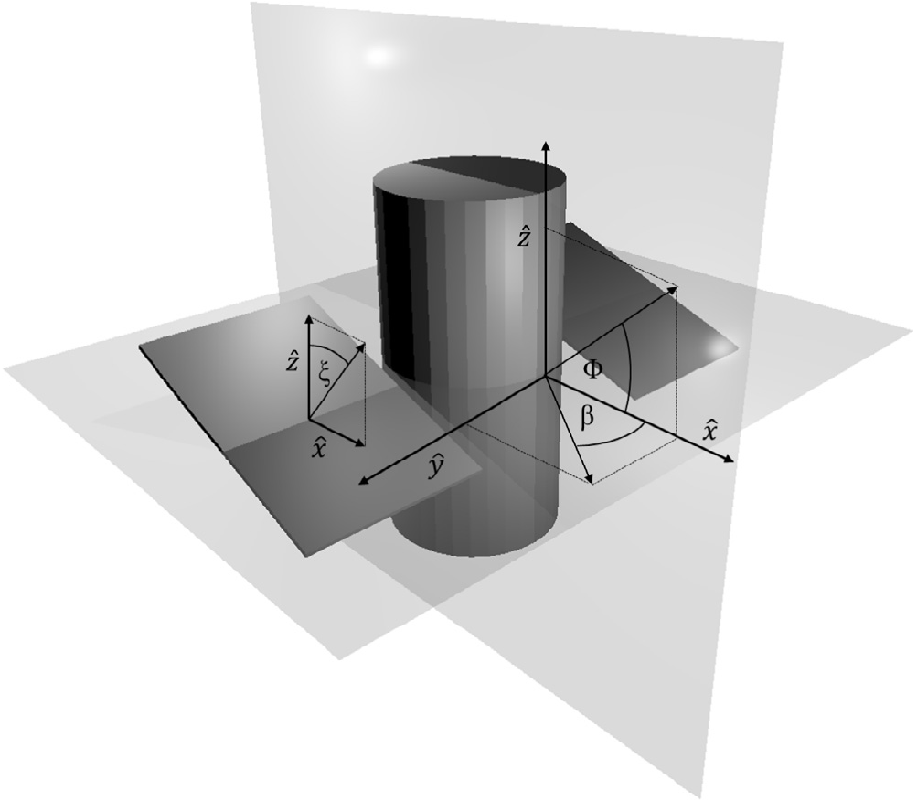
Figure 1: Mesh visuals for the HST (left) and the GRACE (right) satellite.

Figure 1 shows visualizations of mesh files for two satellites, HST on the left and GRACE to the right. Satellite configuration in LEO is modulated by the orientation angles $\theta$ and $\phi$ in Table 1, which have the effect of rotating the meshes. Although each vector on the mesh is technically an input coordinate, meaning that one could take the parameter space to be every degree-of-freedom in the satellite design imaginable, we do not consider that setup in our analysis. It is typical to take the meshes as fixed except in the case of movable features of the satellite such as the panels attached to the HST. We have been provided with ten sets of meshes for HST, from panel angle zero to 90 degrees, in ten degree increments, which effectively creates an eighth “free” input parameter augmenting the seven in Table 1.

We used so-called test particle Monte Carlo (TPMC) method, via a C program developed at Los Alamos National Laboratory, to simulate the environment encountered by satellites for drag coefficient calculations in LEO. TPMC is a computational method used primarily for studying gas dynamics in the free molecular regime where particles have mean-free paths which are much longer than the characteristic lengthscale of the flow. This means that intermolecular collisions can be ignored and TPMC becomes a ray tracing technique that treats each particle independently. In TPMC simulations, the only collisions that matter are those that occur with a surface, such as the surface of a spacecraft. For more details and a comparison to alternative methods, see Appendix A and Mehta et al., (2014a). TPMC takes in a mesh file, settings for the free parameters (Table 1), and weights on the chemical species, which we usually provide as unit vectors. TPMC supports several GSIs, but we utilize the CLL throughout. In Appendix A we describe an enhanced implementation leveraging OpenMP parallelization, an R (R Core Team,, 2017) wrapper we call tpm, and features in R for cluster parallelization via the built-in parallel library. Timing information on a modern multicore desktop is also provided for reference. Source code for this implementation, as well as mesh files for a dozen or so satellites including HST, GRACE, and the International Space Station, and data files containing runs from Mehta et al., (2014b) and those involved in our suite of experiments in Section 6, are furnished as supplementary material.

2.1 GP review

A GP is technically a prior over functions (Stein,, 1999), with finite-dimensional distributions defined by a mean $\mu(x)$ and positive definite covariance $\Sigma(x,x^{\prime})$, for $p$-dimensional input(s) $x$ and $x^{\prime}$. For regression applications with $N\times p$ design matrix $X_{N}$ and $N$-vector of responses $Y_{N}$, combined as data $D_{N}=(X_{N},Y_{N})$, that prior implies the multivariate normal sampling model $Y_{N}\sim\mathcal{N}_{N}(\mu_{N},\Sigma_{N})$. Usually, a small number of parameters $\theta$ determine $\mu_{N}$ and $\Sigma_{N}$. For example, linear regression is a special case where $\theta=(\beta,\tau^{2})$, $\mu_{N}=X_{N}\beta$, and $\Sigma_{N}=\tau^{2}I_{N}$.

Whereas the linear case puts most of the “modeling” in the mean, the term GP emulation is typically used when the emphasis is covariance. When modeling computer experiments (e.g., Santner et al.,, 2003) often $\mu_{N}=0$, which is a simplifying assumption we make throughout. Let $K_{\theta}(x,x^{\prime})$ be a correlation function so that $Y_{N}\sim\mathcal{N}_{N}(0,\tau^{2}K_{N})$, where $K_{N}$ is the positive definite matrix comprised of $K_{\theta}(x_{i},x_{j})$ evaluations on pairs of rows of $X_{N}$. Here we are changing the notation slightly, reserving $\theta$ for $K_{\theta}$ and introducing $\tau^{2}$ as a separate scale parameter. Choices of $K_{\theta}(\cdot,\cdot)$ determine properties of the input–output relationship including stationarity, smoothness, differentiability, and the decay of spatial correlation.

A simple first choice is the so-called isotropic Gaussian: $K_{\theta}(x,x^{\prime})=\exp\{-\sum_{k=1}^{d}(x_{k}-x^{\prime}_{k})^{2}/\theta\}$, where correlation decays exponentially fast in the squared distance between $x_{k}$ and $x_{k}^{\prime}$ at rate $\theta$, called the characteristic lengthscale. A more common generalization is a so-called anisotropic or separable Gaussian which uses a separate lengthscale for each input coordinate: $K_{\theta}(x,x^{\prime})=\exp\{-\sum_{k=1}^{d}(x_{k}-x^{\prime}_{k})^{2}/\theta_{k}\}$, with vectorized $\theta=(\theta_{1},...,\theta_{k})$. With these choices the sample paths are very smooth (infinitely differentiable) and the resulting predictor is an interpolator, which is appropriate for many deterministic computer experiments. For smoothing and numerical stability, a nugget can be added to $K_{\theta,\eta}(x,x^{\prime})=K_{\theta}(x,x^{\prime})+\eta\mathbb{I}_{\{x=x^{\prime}\}}$. When a large degree of smoothness is not appropriate, the Matérn family of correlation functions is a common choice (Stein,, 1999), however the software libraries we augment here only support the Gaussian correlation family at this time. Technical aspects of our presentation below are generic to choices of $K(\cdot,\cdot)$, excepting that it be differentiable in all parameters. There are, however, some important computational considerations to do with inference for the unknown parameters which will require some care in the local neighborhood(s) context of Section 2.3.

GP emulation is popular because inference for $(\theta,\eta)$ is theoretically easy, and prediction is highly accurate and, conditionally on $(\theta,\eta)$, analytic. Under the reference prior $\pi(\tau^{2})\propto 1/\tau^{2}$, Berger et al., (2001) provides a marginal likelihood for the remaining unknowns as

$$p(Y_{N}|K_{\theta}(\cdot,\cdot))=\Gamma[N/2](2\pi)^{-N/2}|K_{N}|^{-1/2}\times\left(\psi_{N}/2\right)^{\!-\frac{N}{2}},\;\;\;\;\;\mbox{where}\;\;\;\psi_{N}=Y_{N}^{\top}K_{N}^{-1}Y_{N}.$$ (2)

Derivatives are available analytically and lead to more numerically stable (if not always computationally efficient) Newton-like schemes for maximizing to obtain Maximum Likelihood Estimation (MLE) lengthscale estimates, $\hat{\theta}$, which is our preferred method of inference throughout, unless otherwise noted. The predictive distribution $p(y(x)|D_{N},K_{\theta}(\cdot,\cdot))$, is Student-$t$ with degrees of freedom $N$:

mean: $$\mu(x|D_{N},K_{\theta}(\cdot,\cdot)) =k_{N}^{\top}(x)K_{N}^{-1}Y_{N},$$ (3)

scale: $$\sigma^{2}(x|D_{N},K_{\theta}(\cdot,\cdot)) =\textstyle{\frac{1}{N}}\psi_{N}[K_{\theta}(x,x)-k_{N}^{\top}(x)K_{N}^{-1}k_{N}(x)],$$ (4)

where $k_{N}(x)$ is the $N$-vector whose $i^{\mbox{\tiny th}}$ component is $K_{\theta}(x,x_{i})$. The variance of $Y(x)$ is $V_{N}(x)\equiv\sigma^{2}(x|D_{N},K_{\theta}(\cdot,\cdot))\times N/(N-2)$. Its form will be important later when we discuss local approximation (Section 2.3). Qualitatively, $V_{N}(x)$ is small/zero for $x$ being in the design $X_{N}$ and increasing in a quadratic fashion when moving $x$ away from elements of $X_{N}$.

2.2 Proof-of-concept GP emulation of satellite drag

The reason we are careful to say “if not always computationally efficient” above is because the trouble with all this is $K_{N}^{-1}$ and $|K_{N}|$, appearing in several instances in Eqs. (2–4), usually requiring $\mathcal{O}(N^{3})$ computation and $\mathcal{O}(N^{2})$ storage for dense matrices. That limits data size to $N\approx 5000$ in reasonable time using optimized linear algebra libraries such as the Intel MKL. This limitation led Mehta et al., (2014b) to consider $N=1000$, separately for each of the six pure chemical species, in their Bayesian Markov Chain Monte Carlo (MCMC) setup—posterior sampling requiring orders of magnitude more matrix inversions compared to derivative-based MLE optimization, which implied further limitations on $N$. An $N=1000$-sized space-filling design in the full input space, described in Table 1, leads to an underwhelming predictor. In our own empirical work in Section 6, we show that relative out-of-sample predictive error is upwards of 15%, far off the typical 1% benchmark.

This led Mehta et al., (2014b) towards a more local analysis, focusing on a limited range of the orientation angles in Table 1.

Symbol	ASCII	Parameter	Ideal Range	Reduced Range	Percentage
$\theta$	theta	yaw	$[-\pi,\pi]$	[-0.052313, 0.052342]	1.7%
$\phi$	phi	pitch	$[-\pi/2,\pi/2]$	[1.059e-05, 5.232e-02]	1.7%

Table 2: Reduced ranges for the orientation inputs first described in Table 1.

Table 2 shows the reduced ranges for these two variables. The combined omission of 98.3% for each of two variables results in an input space sized to less than 0.3% of its original volume—even with the other variables continuing to span their entire range. For GRACE, these new limits are reasonable considering that this satellite is attitude stabilized. That range spans actual observed angles over a several-year period. However, other angles may be encountered in the future. For HST, this range is extremely limiting, as the satellite frequently rotates when performing different imaging experiments. Appendix A provides a coded example showing that a space-filling design in this reduced domain (data files are provided as supplementary material) leads to an out-of-sample relative accuracy of 0.73% for GRACE in pure He, beating the 1% benchmark. The results are similar, with nearly identical code, for the other pure chemical species and for HST.

Although these results are promising, there are some obstacles to scaling things up to the full domain, particularly the issue of GPs with large $N$. One option is a patchwork of little-$n=1000$ analyses, but that would require upwards of $N=4$ million runs for each chemical species and would result in a global predictive surface that had hard breaks between the regions. That could prove problematic when trying to predict jointly for an orbital trajectory through the input space spanning the disjoint regions, i.e., spanning more than 1.7% of either of the orientation angles. However, the spirit of local analysis has merits.

2.3 Local approximate Gaussian processes

The limitation of GP modeling with moderate/large $N$ is not an exactly new problem in the literature. However as data sets have become ever larger over time, research into remedies, via approximation, has become ever more frenzied. Inducing sparsity in the covariance structure is a recurring theme. For a review, see Gramacy and Apley, (2015) which describes the foundation of the methodology we prefer for the satellite drag problem as its emphasis is on local sub-problems. Specifically, it is faithful to the spirit of Mehta et al., (2014b)’s data-subsetting approach but without hard breaks. Both can also be seen as leveraging sparsity, but in fact only work with small dense matrices. Both also involve statistically and algorithmically independent calculations, and thus facilitate massive parallelization. They differ, however, in how they define the local data subsets. Whereas Mehta et al., (2014b) would divvy up the space in terms of the orientation inputs, Gramacy and Apley, offer a more fluid notion of locale.

The idea centers around deriving approximate predictive equations at particular generic location(s), $x$, via a subset of the data $D_{n}(x)\subseteq D_{N}$, where the sub-design $X_{n}(x)$ is (primarily) comprised of $X_{N}$ close to $x$. The reason is that, with the typical choices of $K_{\theta}(x,x^{\prime})$, where correlation with elements $x^{\prime}\in X_{N}$ decays quickly for $x^{\prime}$ far from $x$, remote $x^{\prime}$ have vanishingly small influence on prediction. Ignoring them in order to work with much smaller, $n\times n$, matrices brings big computational savings with little impact on accuracy. Although an exhaustive search for the best $n$ out of $N$ things is combinatorially huge, Gramacy and Apley, show how a greedy search can provide designs $X_{n}(x)$ where predictors based on $D_{n}(x)$ furnish local predictors which are at least as accurate as simpler alternatives (such as nearest neighbor (NN)) yet require no extra computational time.

Their greedy search starts with a small nearest neighbor set $D_{n_{0}}(x)$, and then, successively chooses $x_{j+1}\in X_{N}\setminus X_{j}(x)$ to augment $X_{j}(x)$ and form $D_{j+1}(x)$ according to one of several simple objective criteria. The criterion they prefer, approximately minimizing an estimate of mean-square prediction error, involves choosing $x_{j+1}$ to maximize the reduction in variance at $x$:

$$v_{j}(x ;\theta)-v_{j+1}(x;\theta),\quad\mbox{(dropping $\theta$ below)}$$ (5)

$$=k_{j}^{\top}(x)G_{j}(x_{j+1})v_{j}(x_{j+1})k_{j}(x)+2k_{j}^{\top}(x)g_{j}(x_{j+1})K(x_{j+1},x)+K(x_{j+1},x)^{2}/v_{j}(x_{j+1}),$$

where $G_{j}(x_{j+1})\equiv g_{j}(x_{j+1})g_{j}^{\top}(x_{j+1})$, and $g_{j}(x_{j+1})=-K_{j}^{-1}k_{j}(x_{j+1})/v_{j}(x_{j+1})$. To recognize a similar global design criterion called active learning Cohn (Cohn,, 1996), Gramacy and Apley, called this criterion ALC. They demonstrate that building local designs in this way with small $n$, say $n=50$, takes fractions of a second even with $N$ in the tens of thousands, say $N=4\times 10^{4}$, and the predictions are highly accurate. Inverting a $(4\times 10^{4})\times(4\times 10^{4})$ matrix is not possible on most modern desktops because of memory swapping issues. For a point of reference, inverting a $(4\times 10^{3})\times(4\times 10^{3})$ matrix on a modern desktop takes about five seconds.

The $\mathcal{O}(n^{3})$ calculations above are independent for each $x$, so predicting over a dense grid of locations $x\in\mathcal{X}$ is trivially parallelizable. Shared memory parallelization, exploiting now-standard multi-core desktop architectures, proceeds in C via one additional line of code: pragma omp parallel for placed above the serial for over $x\in\mathcal{X}$. That statistical independence can also be leveraged to obtain a nonstationary effect by independently fitting local lengthscales to the local designs at each $x$. Global predictors so-derived tend to be more accurate than local ones sharing a common lengthscale, and better than global full-GP ones when those can feasibly be calculated. A comprehensive suite of benchmarking results on laGP variations can be found in the literature (e.g., Gramacy and Apley,, 2015; Gramacy et al.,, 2014; Gramacy and Haaland,, 2015; Gramacy,, 2016).

We note two caveats here, which are important for our applied work. One is that although Gramacy and Apley, developed their theory generic to the correlation structure, in fact, their initial implementation in the laGP package Gramacy and Sun, (2018); Gramacy, (2016) only supported an isotropic version owing to the peculiarities of R’s internal optimization subroutines. Those routines use static C variables which are not thread-safe, meaning that separable covariance MLE calculations could not (easily) occur in parallel. Using somewhat elaborate OpenMP pragmas we were able to largely circumvent this issue with an update to laGP. As we illustrate in Sections 5–6, these enhancements are essential for good performance in many benchmark problems and for our satellite drag application, in particular. We view this as a substantial technological innovation if not a traditionally methodological one. The other caveat is that building up local designs $X_{n}(x)$ requires iterating over all $N-j$ remaining candidates in $X_{N}\setminus X_{j}(x)$ in search of each $x_{j+1}$. This can be quite expensive when $N$ is big. Gramacy and Apley, suggest limiting the search to a set of $N^{\prime}$ nearest neighbors, where $n\ll N^{\prime}\ll N$. However this is somewhat unsatisfying, and is particularly disadvantageous in the context of our proposed trajectory-wise extensions to local design search in Section 4.

3 Multiresolution global/local GP emulation

As we illustrate in our drag emulation empirical work in Section 6, laGP is able to accommodate much larger data sets and thereby drive down relative out-of-sample prediction error substantially compared to the 10-15% global GPs can accomplish based on N in the small thousands. The technological ability to circumvent the thread-safety issue in order to efficiently fit local anisotropic covariance structures (in parallel) leads to substantial improvements over the existing locally isotropic capability. However, even with N as big as 2 million runs, its predictions are unable to meet the 1% benchmark error rate, being at best upwards of 2.5%. Generating even larger data sets is an option, potentially requiring a doubling of the simulation effort which already stands at seventy thousand core hours. Here we outline a simple hierarchical approach to global/local emulation that offers big improvements on accuracy without larger design, ultimately substantially beating the 1% benchmark.

The idea involves recognizing that a sparsity-inducing correlation structure biases fits towards local effects. This is well known in the literature, and remedies abound. For example, Kaufman et al., (2012) compensate by utilizing a low degree Legendre polynomial basis in the mean structure of the GP. Unfortunately this idea is not easily extended to laGP since joint (and fully Bayesian) inference for mean and residual spatial structure would break the independent, and thus easily parallelized, nature of the calculations (and MCMC would prohibitively limit data sizes). In any case, as we show in Appendix B on much more modestly-sized examples, that approach is uncompetitive on accuracy grounds (ignoring computation) relative to what we propose here, even though there are many similarities, at least in spirit. The basic idea is to first fit a global GP, rather than a basis-expanded mean, and use that fit to set up a more appropriate (and primed) local (sparsity-inducing) prediction problem. We show in several variations [Appendix B, Sections 5 and 6] that this leads to highly accurate, and computationally tractable predictors in a large $N$ setting.

3.1 Bootstrapped block Latin hypercube subsamples

The idea is to first obtain global lengthscale estimates, $\hat{\theta}$, rather than a global predictor, even though our ultimate goal is prediction. Liu and Hung, (2015) demonstrate that a global lengthscale for the separable GP can be efficiently estimated via MLE calculations on manageably-sized data subsets. The simple option of random subsetting works well in practice, but does not offer theoretical guarantees. Intuitively, simple random subsampling fails to ensure that the spectrum of pairwise distances in the subsample reflects that of the original data set. Liu and Hung, show that a so-called block-bootstrap Latin hypercube subsampling (BLHS) strategy can yield global lengthscales which are consistent with the full data MLE under increasing domain asymptotics. Basically, the BLHS guarantees a good mix of short and long pairwise distances. The method is similar in flavor to so-called full scale approximation (Sang and Huang,, 2012; Zhang et al.,, 2015). It also has aspects in common with composite likelihood approaches (Varin et al.,, 2011; Gu and Berger,, 2016). Yet BLHS is simpler both conceptually and in implementation, in part because it offers far less—only consistent lengthscales. The ingredients are: (1) a block Latin hypercube (LH) subsample routine; (2) a GP fitting library; (3) a for loop. Items (2) and (3) are easy. Our blhs in the laGP package, following Liu and Hung,’s description provided below, is just 35 lines of R code.

A single BLHS in $d$ dimensions may be obtained by dividing each dimension of the input space equally into $m$ intervals, yielding $m^{d}$ mutually exclusive hypercubes. The average number of observations in each hypercube is $Nm^{-d}$ if there are $N$ samples in the original design. From each of these hypercubes, $m$ blocks are randomly selected following the LH paradigm, i.e., so that only one interval is chosen from each of the $m$ segments. The average number of observations in the subsample, combining the $m$ randomly selected blocks, is $Nm^{-d+1}$. Ensuring a subsample size $\geq 1$ requires having $m\leq N^{\frac{1}{d-1}}$, thereby linking the parameter $m$ to computational effort. Smaller $m$ is preferred so long as GP inference on data of that size remains tractable. Since the blocks follow a LH structure, the resulting sub-design inherits the usual LHS properties, e.g., retaining univariate stratification modulo features present in the original, large $N$, design. The computational cost to estimate lengthscale via BLHS is $\mathcal{O}({n^{\star}}^{3})$, where $n^{\star}=Nm^{-d+1}$.

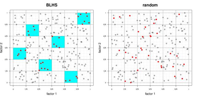
Figure 2: A visual comparison of the BLHS based subsample (left) and a random subsample (right), both derived from an original sample from a LHS. The original $N$-sized design locations are shown as open circles, cyan-filled areas are the randomly chosen blocks, and the red-filled dots indicate the random subsample.

As an example, consider the left panel of Figure 2 where we have $N=216$, $d=2$, and have chosen $m=6$. All together there are $m^{d}=36$ hypercubes, which are outlined by black dashed lines. The cyan-filled areas correspond to the selected blocks, and the red dots are the resulting subsamples. It is clear that the selected samples have desirable space-filling properties. Observe that—compared say to the random subsample exemplified by the right panel in the figure—the BLHS guarantees short and long pairwise distances.

Subsample in hand, one can efficiently obtain estimated lengthscale parameters via typical MLE calculations. Figure 3 anticipates some of our later empirical work by illustrating the bootstrap distribution of estimated lengthscales for the classic borehole problem (left) and HST in pure He (right) (For more details on the experimental setup, see Section 5.1 and 6.1, respectively.).

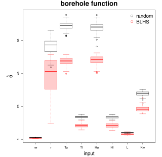
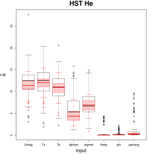
Figure 3: Comparing MLE lengthscale parameters obtained via BLHS and random subsampling. The left panel corresponds to the borehole example (see Section 5), using $N=10^{5}$ and $n=Nm^{-d+1}=781$ with $m=2$ and $d=8$; the right panel is HST in pure He with $N=10^{6}$ and $n=Nm^{-d+1}=457$ with $m=3$ and $d=8$.

Details such as data sizes $N$ are provided in the figure caption, and $m$ was chosen as small as possible, yet yielding a subsample with less than $1000$ runs. To ensure a fair comparison, random subsample sizes were chosen to match their BLHS counterparts. Observe that, in both cases, the lengthscales estimated under BLHS are consistently smaller than the ones under random subsampling, with differences being particularly stark for the borehole example. Intuitively, this is due to the larger degree of short pairwise distances in the BLHSs. Theoretically, we know that the BLHS estimates are asymptotically consistent, and therefore the random subsample ones must be biased. Also observe that estimates under random subsampling for HST have a long right-hand tail. This suggests that when extracting point estimates from the random samples, medians are preferred over means.

3.2 From global lengthscales to local prediction

Having a computationally tractable method for estimating lengthscales is important, but not directly useful in many settings where GP surrogates are typically deployed. Liu and Hung, (2015) developed BLHS in order to perform variable selection on a parametric modeling component, which is not really relevant to our emulation problem. Although lengthscale estimation may have avoided expensive $\mathcal{O}(N^{3})$ computation, prediction conditional on those parameters still requires large matrix decompositions (see, e.g., Eq. (3)).

This is where laGP comes in. One option would be to condition laGP on these estimated global lengthscales $\hat{\theta}^{(g)}$, rather than an otherwise arbitrary default value $\theta^{(0)}$. However this is equivalent to scaling the input coordinates as $x_{ij}/\sqrt{\theta_{j}^{(g)}}$, for both training and testing locations, and initializing with a lengthscale of $1$ for all coordinates. We prefer this latter option from an implementation perspective, considering how laGP derives default priors, parameter ranges, and other MLE-calculating specifications. Then laGP calculations can proceed as usual. Inferring local lengthscales, with the search initialized at $1$, produces a kind of multiresolution effect: the local design $X_{n}(x)|\hat{\theta}^{(g)}$ is determined by the global lengthscale, and subsequent local estimation of the $\hat{\theta}(x)|D_{n}(x)$, is determined by the observations at that local design: $D_{n}(x)=\{X_{n}(x),y(X_{n}(x))\}$.

Pre-scaling with suitably estimated global lengthscales enhances numerical stability and efficiency, by priming the local optimizer, and tailors local adjustments (to both $D_{n}(x)$ and $\hat{\theta}(x)$) to a globally inferred reference $\hat{\theta}^{(g)}$ rather than one-size-fits-all default $\theta^{(0)}$. Even in the special case of NN local design, the $X_{n}(x)$ in the re-scaled space “feel” the effect of the global lengthscale. Back on the original scale of the inputs, the distances upon which “nearest” is judged are no longer Euclidean. By down-weighting inputs with longer lengthscales, the effect is akin to utilizing a Mahalanobis distance (Bastos and O’Hagan,, 2009) but without the prohibitive $\mathcal{O}(N^{3})$ computational cost that that would entail.

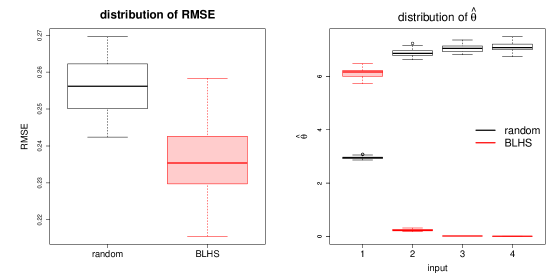
Figure 4: Comparing RMSE (left) and MLE lengthscales (right) on simulated Michalewicz data obtained via BLHS and random subsampling, respectively, using $N=5\times 10^{4}$ and $n=Nm^{-d+1}=781$ with $m=4$ and $d=4$.

The left panel of Figure 4 shows a root-mean-squared-error (RMSE) distribution, and the right panel shows MLE lengthscales for $N=5\times 10^{4}$ LHS, both on the Michalewicz function [Section 5.2], with $p=4$ and $M=10$. The RMSEs reported were obtained by predicting on a testing set of size $1000$, and employing the global-local hybrid laGP described above. Section 5.2 offers more details, and an expanded comparator set for this example. Observe that the distribution of RMSEs is clearly more favorable for BLHS compared to random subsampling. Looking at the MLEs, three of the four inputs exhibit the same feature as in the borehole data: the random subset ones are biased high. The first input is the other way around, however. One might speculate that gross over-estimates for the latter three inputs may have contributed to overcompensation in the first.

One of the advantages of the Michalewicz function, over say the borehole, is that one can easily generate variations based on the input dimension, $p$. For example, we can empirically study MLE of lengthscale parameters under $p\in\{2,4,6,8\}$ with a sensible data size counterpart $N\in\{10^{4},5\times 10^{4},10^{5},10^{6}\}$ to acknowledge how volume increases quickly with dimension. Tables 3–4 summarize the results from just such an experiment.

$p$	method	quantile
		5 %	50 %	95 %
2	BLHS	3.18e-05	3.36e-05	3.83e-05
2	random	3.30e-05	3.48e-05	3.72e-05
4	BLHS	0.225	0.235	0.250
4	random	0.246	0.256	0.266
6	BLHS	0.477	0.494	0.512
6	random	0.524	0.540	0.562
8	BLHS	0.641	0.655	0.675
8	random	0.652	0.673	0.708

Table 3: Distribution of RMSEs. Each column, from left to right, shows the dimensionality, subsampling method, and quantile information of RMSEs (5%, 50%, and 95%, respectively). Each row is composed of two sub-rows, each of which shows the quantile distribution using the specific subsampling method under certain dimensionality.

Table 3 continues where the left panel of Figure 4 left off, detailing the distribution of RMSEs for varying dimension $p$ and sample size $N$. Observe that BLHS consistently outperforms random subsampling in this exercise, excepting the upper 95% quantile for $p=2$.

method	quantile	lengthscale in each coordinate
		1	2	3	4	5	6	7	8
BLHS	10 %	0.0087	0.0024
BLHS	50 %	0.0088	0.0024
BLHS	90 %	0.0089	0.0024
random	10 %	0.0107	0.0029
random	50 %	0.0108	0.0029
random	90 %	0.0108	0.0029
BLHS	10 %	5.8116	0.1995	0.0207	0.0109
BLHS	50 %	6.1631	0.2299	0.0212	0.0127
BLHS	90 %	6.3919	0.2957	0.0219	0.0142
random	10 %	2.8905	6.7090	6.8810	6.8940
random	50 %	2.9512	6.8596	7.0491	7.0767
random	90 %	2.9987	7.1045	7.2477	7.3142
BLHS	10 %	2.7158	1.1104	4.3722	1.4843	2.8059	4.4307
BLHS	50 %	2.9419	1.3741	4.5539	1.5865	3.0854	4.6223
BLHS	90 %	3.2309	1.5153	4.6883	1.7911	3.5958	4.8184
random	10 %	0.0457	0.0280	0.1874	0.2970	0.3352	0.3366
random	50 %	0.0555	0.0342	0.2467	0.3603	0.3972	0.4050
random	90 %	0.0730	0.0419	0.2907	0.4159	0.4290	0.4526
BLHS	10 %	4.6204	2.4794	5.5265	2.8159	4.8700	5.5874	5.8449	6.1936
BLHS	50 %	4.8334	2.7317	5.8004	3.1132	5.1314	5.8291	6.0473	6.2677
BLHS	90 %	5.0122	2.9202	5.9439	3.3995	5.2812	6.0269	6.1813	6.4472
random	10 %	0.0581	0.2794	0.3801	0.4269	0.4267	0.4641	0.4456	0.4742
random	50 %	0.0805	0.3436	0.4429	0.4824	0.5100	0.5230	0.5166	0.5472
random	90 %	0.0930	0.3928	0.4823	0.5616	0.5879	0.5996	0.5935	0.6627

Table 4: Distribution of $\hat{\theta}$. Each column, from left to right, shows the subsampling method, quantile information, and $\hat{\theta}$ under different dimensionality. Each row is composed of two big sub-rows, each of which shows the quantile distribution (10%, 50%, and 90%) using the specific subsampling method under certain dimensionality.

Table 4 focuses on lengthscales estimated from that experiment, this time summarizing boxplots numerically (like in the right panel of Figure 4) for varying input dimension $p$. Notice how BLHS estimates differ from those from random subsampling. When $p=2$, the BLHS estimates are consistently smaller at each quantile. However the pattern is exactly the opposite when $p=8$. The pattern for $p=4$ was already discussed above.

4 Joint path sampling

Obtaining predictions over a dense global input “grid” $\mathcal{X}$ may be overkill in many settings. For example, we are rarely interested in drag coefficients for satellites like the HST positioned anywhere in orbit or in arbitrary orientation. Rather, it is far more useful to be able to understand drag at potential nearby locations and configurations in space and time. A satellite’s trajectory in the input space is limited to $x^{\prime}s$ near its current configuration, $x_{0}$ say, since aspects like velocity and orientation can not be altered instantaneously, and others like temperature and chemical composition evolve slowly and smoothly in time and space. Our LANL colleagues desire joint predictions along paths $\mathcal{W}(x_{0})\subset\mathcal{X}$ in the input space emanating from $x_{0}$ values. Yet laGP is an inherently pointwise procedure. Although it derives its speed from parallelization, via statistical and computational independence, that comes at the expense of punting on a joint predictive capability. Here we develop a new criterion for sub-design local to a set, alongside methods for finding solutions efficiently.

4.1 An aggregate criterion

Consider a fixed, discrete and finite set of input locations $W\subset\mathcal{X}$, perhaps specified by the practitioner, or derived from a satellite’s current trajectory/flight plan in the motivating drag context. Let $k_{j}(w)$ denote the $j\times 1$ correlation vector for each $w\in W$. As described above, we target $W\equiv\mathcal{W}(x_{0})$ as satellite trajectories, but the development here is for a generic set $W$ with potential for wider application. The extension of our reduction in variance (ALC) criterion $v_{j}(x)-v_{j+1}(x)$, from Eq. (5), is

$$v_{j}(W)-v_{j+1}(W)=\frac{1}{|W|}\sum_{w\in W}\left\{v_{j}(w)-v_{j+1}(w)\right\},$$ (6)

$$=\frac{1}{|W|}\sum_{w\in W}\left\{k_{j}^{\top}(w)G_{j}(x_{j+1})v_{j}(x_{j+1})k_{j}(w)+2k_{j}^{\top}(w)g_{j}(x_{j+1})K(x_{j+1},w)+\frac{K(x_{j+1},w)^{2}}{v_{j}(x_{j+1})}\right\}.$$

Observe that this quantity is a scalar, measuring the average reduction in predictive variance over $W$, which we wish to maximize over the choice of new $x_{j+1}$. With our trajectory application in mind, we refer to Eq. (6) interchangeably as a “joint” and/or “path” ALC criterion.

As an illustration of sequential design under the criterion in Eq. (6), consider a two-dimensional $\mathcal{X}\in[-2,2]^{2}$ and $W$ comprised of a path of locations $w(x)=(x-0.75,x^{3}+0.51)$ with $100$ $x$-values ranging uniformly in $[-0.85,0.45]$. The response, and other details, are described in Gramacy and Apley, (2015, Section 3.4), but are not particularly germane here.

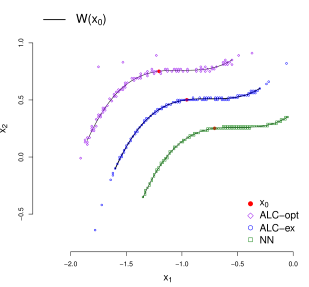
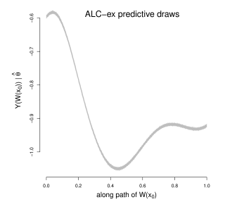
Figure 5: The left panel shows local designs under three criteria (shifted for visibility) for identical paths $\mathcal{W}(x_{0})\in[-2,2]^{2}$, respectively; the right panel shows predictive samples along $\mathcal{W}(x_{0})$ corresponding to one of the three designs (the other two are nearly identical). The point labeled $x_{0}$ is the midpoint along the path.

Figure 5 shows local designs of size $n=100$ from an $N\approx 4\times 10^{4}$-sized grid, and predictive samples along that path. The left panel shows two “path” ALC-based local designs, i.e., following Eq. (6), and one NN-based design, with plots shifted for visibility. The NN sub-design is comprised of elements of the data grid which are closest in Euclidean distance to any element of $W$. The sub-design labeled ALC-ex was found in a manner similar to ordinary pointwise ALC search where every location (limited to the $N^{\prime}=10^{4}$ locations closest to $W$) is entertained, in turn, at each iteration of the sequential design search, at substantial computational expense. Observe the clear distinction with the much thriftier NN-based sub-design: it has fewer neighbors and more satellite points. The ALC-opt set will be discussed momentarily.

The right panel in Figure 5 shows $1000$ sample paths from the local design along the path under the “joint” ALC criterion, illustrating its value over an independent pointwise alternative. Pointwise sampling could not generate such sample paths, lacking a full predictive covariance structure. Only one set of samples is shown, with the ones for the other two methods being strikingly similar. However, as we show shortly, the three approaches do not always predict equally well over a collection of many diverse predictive paths.

An exhaustive search for $X_{n}(W)\subset X_{N}$, where $X_{n}(W)$ denotes the local design for $W$, following the new path criterion in Eq. (6) (ALC-ex in the figure) is more computationally expensive than the pointwise analog $X_{n}(x)$ (Eq. 5) for two reasons. One reason is that the former makes $m$ ($=100$ in our example) calculations where the latter makes one. The other is that, relative to a single point $x$, a path $W$ traversing a swath of the input space demands inspecting a larger portion of $X_{N}$. That is, a larger searching set $N^{\prime}$ is needed. Using the nearest $N^{\prime}=10^{3}$ in our example above is too small, excluding about 10% of the points selected via ALC(s). Combined, those multiple orders of magnitude increase in computational expense represent a heavy burden that we shall quantify shortly.

4.2 Derivative-based ALC search

Towards lighter-weight sub-design search we considered swapping out exhaustive enumeration (a discrete search) with a continuous analog utilizing derivatives. This is similar in spirit to the ray-based search of Gramacy and Haaland, (2015) for pointwise local designs at each $x$. Rays, however, would not be suitable for exploring over joint characteristics for sets $W$. Although our ultimate usage will be for paths $\mathcal{W}(x_{0})$, we note that these derivatives may also be used for pointwise search, however the computational savings may not be as impressive as the ray-based alternative in that setting.

Below we provide the expression for the components of the gradient of the extended ALC expression in Eq. (6), assuming a separable covariance structure. For $\ell=1,\dots,p$

$$\frac{\partial}{\partial(x_{j+1})_{\ell}} \left\{v_{j}(W)-v_{j+1}(W)\right\}$$ (7)

$$= \frac{1}{|W|}\sum_{w\in W}\left\{-2k^{\top}_{j}(w)K^{-1}_{J}\left[\frac{\partial k_{j}(x_{j+1})}{\partial(x_{j+1})_{\ell}}+\frac{k_{j}(x_{j+1})a}{v_{j}(x_{j+1})}\right]b-abc+2c\frac{\partial K(x_{j+1},w)}{\partial(x_{j+1})_{\ell}}\right\},$$

where the macros $a$, $b$ and $c$ (all scalars) are

$$a =2\frac{\partial k_{j}^{\top}(x_{j+1})}{\partial(x_{j+1})_{\ell}}K_{j}^{-1}k_{j}(x_{j+1}), b =g_{j}^{\top}(x_{j+1})k_{j}(w)-K(x_{j+1},w)/v_{j}(x_{j+1}),$$

and $$c =g_{j}^{\top}(x_{j+1})k_{j}(w)+K(x_{j+1},w)/v_{j}(x_{j+1}).$$

A detailed derivation is provided in Appendix C. Simplifications arise under an isotropic lengthscale, via a single derivative calculation rather than the $p$ components of a gradient, $\ell=1,\dots,p$. Any correlation family may be used so long as derivatives may be calculated relative to the spatial locations, $x$, e.g., for $\frac{\partial}{\partial(x_{j+1})_{\ell}}k_{j}^{\top}(x_{j+1})$, which is straightforward for the typical power exponential (Gaussian) and the Matérn families.

Derivative in hand, we turn to numerical optimization using L-BFGS-B (Byrd et al.,, 1995), a quasi-Newton method implemented in the optim library for R. Owing to the linear nature of variance reduction in Gaussian models as the sample size $n$ increases (particularly with nearby locations in GP prediction), the magnitude of the reduction in variance criterion like Eq. (6) becomes numerically tiny as $n$ grows, easily matching typical convergence tolerances like $10^{-8}$, even when $n$ as small as $20$, which can result in premature convergence of the numerical optimizer. Instead, supplying the logarithm of the criterion as an objective to optim—along with the derivative of the $\log$ which may be calculated as a ratio of the derivative and the original criterion—leads to better behavior. The numerator and denominator in ratio comprising the log derivative may involve small numbers which can result in “extra” iterations of the solver close to convergence. We have found that these can be avoided by supplying a larger pgtol argument which controls an aspect of the stopping rule determined by ineffective line searches in the L-BFGS-B algorithm.

Our use of optim and the derivative replaces an exhaustive discrete search with a continuous one, providing a solution $x^{\ast}_{j+1}$ which is “off” the candidate set $X_{N}$. So the final step involves “snapping” $x^{\ast}_{j+1}$ onto $x_{j+1}\in X_{N}\setminus X_{j}(W)$, by minimizing Euclidean distance. It is worth noting that the result is not guaranteed to be a global minimum of the ALC surface. A multi-start scheme could be employed, however, we find that this does not offer a good cost-benefit trade-off in terms of computational effort. Rather, we developed an initialization scheme for the solver which recognizes the sequential nature of our sub-design search, over the iterations $j=n_{0},\dots,n$, via a round-robin on NN similar to Gramacy and Haaland, (2015). Specifically, we maintain a stack of starting locations from $X_{N}$ which are sorted via (minimum) distance to $W$. To start a search for the next $x_{j+1}$, the next initializer is popped off. If the $x_{j+1}$ thus found matches any (remaining) stack element, it too is popped off to prevent it from initializing future searches. Although this scheme does not guarantee global optima, for each individual search or for the final local design $X_{n}(W)$, it has the advantage of being deterministic. We find that it leads to local designs that are just as good as the exhaustive search on average and, most importantly, are better than NN.

Before turning to empirical results, let’s revisit our illustration in Figure 5. The design denoted as ALC-opt in the left panel corresponds to the derivative-based search described above. Observe that this local design is qualitatively similar to the exhaustive one, having more satellite points and fewer neighbors than the NN version. In this instance, ALC-opt’s satellite points differ from ALC-ex’s, but that is not always the case.

4.3 Empirical results

Here we compare out-of-sample performance for laGP predictors based on the following local design schemes: ALC-opt, ALC-ex, NN, the original ALC criterion (Eq. (5)) applied pointwise (ALC-pw), and NN-pw. We utilize two metrics: Mahalanobis distance, $\sqrt{(y-\mu)^{\top}\Sigma^{-1}(y-\mu)}$, where $\mu$ is a predictive mean vector with components from Eq. (3), and $\Sigma$ is the predictive covariance matrix whose diagonal is in Eq. (4); and RMSE, which follows the same formula but with $\Sigma^{-1}=\mathrm{Diag}(1/N)$. Although RMSE is more conventional, Mahalanobis distance is emerging as the gold standard for data arising from deterministic computer simulation where predictive accuracy and covariance structure are equally important (Bastos and O’Hagan,, 2009). In both cases, smaller is better.

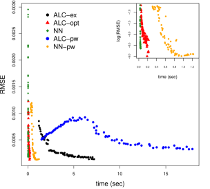
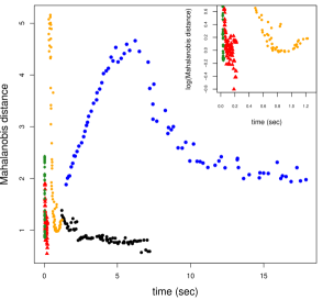
Figure 6: Comparing RMSEs (left) and Mahalanobis distances (right) versus time; smaller is better. Comparators: joint NN, pointwise NN (NN-pw), joint ALC (‘ex’haustive and derivative-based ‘opt’imization), and pointwise ALC (ALC-pw). Zoomed-in glimpses of the lower left of each plot are provided in log space to better visualize separation.

Our first experiment involves the predictive line from Figure 5 with local designs of increasing size, $n=25,\dots,100$, and thus increasing computational effort. Figure 6 shows RMSEs (left) and Mahalanobis distances (right) versus wall-clock time. Excepting ALC-pw and NN-pw, observe how the comparators’ accuracy tends to improve with added time. Also notice that NN and ALC-opt are much faster than the other comparators: it takes relatively little additional computational effort to grow the design and improve out-of-sample performance. Achieving the same gains via exhaustive search, however, brings seriously diminishing returns. Otherwise, i.e., ignoring time, the ALC-ex and ALC-opt searches give about the same out-of-sample performance for fixed local design size. The strikingly poor performance of ALC-pw and NN-pw can be attributed to a number of factors. The most important factor may be the (statistical) independence of calculations involving inherent estimation risk which is mitigated by the joint designs. These two pointwise design schemes perform exceedingly poorly via Mahalanobis distances since a zero off-diagonal covariance is a gross underestimate of the true underlying structure.

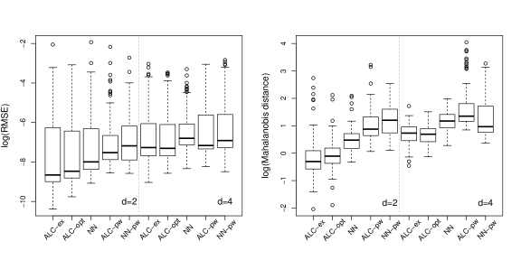
Figure 7: Comparing RMSEs and Mahalanobis distances among ALC-ex, ALC-opt, NN, ALC-pw, and NN-pw. The left panel shows boxplots of log RMSEs based on $100$ random paths; the right panel shows boxplots of log Mahalanobis distances.

Our second experiment holds the local design size fixed (at $n=100$) and varies the two-dimensional lines comprising the set(s), $\mathcal{W}(x_{0})$, in order to more completely span the input space and the space of sets, with the satellite trajectory analogy in mind. Appendix D describes how the sets were randomly generated, and shows what they look like (Figure 15). We consider the distribution of RMSEs and Mahalanobis distances obtained from $100$ predictions on $100$ such lines separately in two and four input dimensions. In the latter four-dimensional (4d) case, the two input dimensions on which the line $\mathcal{W}(x_{0})$ was varied were chosen at random, and the output is derived as the product of two independent two-dimensional (2d) ones. Figure 7 summarizes the results in terms of log RMSE and log Mahalanobis distance. A vertical dashed line separates 2d and 4d experiments. Observe that these results are largely in line with the previous experiment: the joint ALC methods (ALC-ex and ALC-opt) beat the pointwise methods (ALC-pw and NN-pw) to a significant extent. The pattern is more distinct at the lower end of the ranges, with outliers at the top end arising from predictive paths with a substantial component outside the range of the training data, requiring extrapolation.

5 Benchmark and synthetic results

Here we focus on pointwise prediction on two benchmark data sets from the Virtual Library of Simulation Experiments (Surjanovic and Bingham,, 2014), anticipating similar experiments on satellite drag in Section 6. Eighteen comparator variations are trained on $N=10^{5}$ and $N=10^{6}$ runs, paired with testing sets of size $10^{4}$. Sixty such training and testing pairs are generated jointly via LHS, to create a thirty-replicate Monte Carlo experiment comprising a total of 36 variations. The comparators combine a choice of local sub-design (one of “nn”, “alc” and “alc2”, with the latter being a second stage of ALC design as recommended by Gramacy and Apley, (2015)), paired with a choice of correlation structure (either isotropic or separable—“sep”), and a choice of global pre-processing of lengthscale as described in Section 3.1 (either none, random subset—“s”, or a BLHS subset—“sb”).

Although many aspects of the two experiments are similar, variations in the input dimension necessitated some customizations. Our first experiment, on the borehole function (more details in Section 5.1), is in eight dimensions. To have manageable BLHS sizes we chose $m=2$ for the $N=10^{5}$ version, leading to a global subset of size $n=781$; for $N=10^{6}$ we used $m=3$ yielding $n=457$. Choosing $m=2$ for this latter case would have produced $n=7812$, too big for fast GP inference. Similarly, for the Michalewicz function (see Section 5.2), in four dimensions we chose $m=12$ ($n=578$) for $N=10^{6}$, and $m=6$ ($n=462$) for $N=10^{5}$.

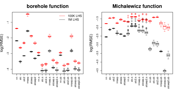
Figure 8: Comparing laGP variations on borehole (left) and Michalewicz (right) functions.

Figure 8 contains boxplots summarizing out-of-sample RMSE for both experiments, with discussion following shortly. The comparators along the $x$-axis are blocked in groups of six from left to right, first without global scaling, and then random or BLHS subsets. Black boxplots correspond to the larger experiment ($N=10^{6}$), which are uniformly lower than the red ones: more training data means more accurate predictions.

5.1 Borehole experiment

The borehole function is a classical example from the computer experiments literature (Morris et al.,, 1993) with inputs in eight dimensions. The response $y$ is given by

$$y=\frac{2\pi T_{u}\left[H_{u}-H_{l}\right]}{\log\left(\frac{r}{r_{w}}\right)\left[1+\frac{2LT_{u}}{\log\left(r/r_{w}\right)r^{2}_{w}K_{w}}+\frac{T_{u}}{T_{l}}\right]}$$

where the inputs are constrained to lie in a rectangular domain:

$$r_{w}\in[0.05,0.15],\qquad r\in[100,5000],\qquad T_{u}\in[63070,115600],\qquad T_{l}\in[63.1,116]$$

$$H_{u}\in[990,1110],\qquad H_{l}\in[700,820],\qquad L\in[1120,1680],\qquad K_{w}\in[9855,12045].$$

Before any modeling, we scale the inputs to lie in the unit cube.

The distribution of $\log(\mathrm{RMSE})$ obtained for our comparators on this borehole data is shown in the left panel of Figure 8. There are several noteworthy results. First, global pre-scaling (whether by random subsets or BLHS, shown by the latter $12$ boxplot pairs) outperform their counterparts without scaling (first six). Second, BLHS-based subsets (latter six) slightly outperform random subsets (middle six). This result is consistent across all local models, but the discrepancy is marginal. Third, observe that NN-based local modeling is poor, with separable correlation kernels being surprisingly poor in each pre-processing regime. The overall best comparator is “alc.sb” which corresponds to BLHS-based pre-scaling and a single application of ALC-based isotropic modeling. Apparently, global estimates of lengthscale are sufficient to capture local scaling. Finally, observe that a second stage of ALC design (comparators with a “2”) is not consistently better than the first stage alone.

A referee requested further experimentation in order to compare with other libraries, primarily in a smaller-$N$ setting. Those results and discussion may be found in Appendix E.

5.2 Michalewicz experiment

The Michalewicz function is widely used in the optimization literature (Molga and C.,, 2005). One unique feature is that it can be defined in arbitrary input dimension, $p$:

$$f(x)=-\sum_{i=1}^{p}\sin(x_{i})\sin^{2M}\left(\frac{ix_{i}^{2}}{\pi}\right),\quad\mbox{ where }x\in\mbox{[0, $\pi$]}.$$

Larger values of the parameter $M>0$ yield steeper transitions in the output space. Figure 9 shows two examples where $(p=1,M=4)$ and $(p=2,M=10)$. There are $p!$ local minima, so the response surface is quite complex under high dimensionality, especially when $M$ is also large. In the experiment we report here, we used $p=4$ and $M=10$.

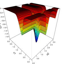
Figure 9: The Michalewicz function. The left panel shows the surface with $(p=1,M=4)$, whereas the right panel corresponds to $(p=2,M=10)$.

The right panel of Figure 8 shows the distribution of $\log(RMSE)$ obtained in that setting. Although the results bear some similarity to the borehole experiment, there are some nuances worth attention. First, a general global pre-scaling is no longer as powerful as before. For example, consider the RMSEs for comparators whose names ended with “s”, which are based on random subsets. These underperform their counterparts without scaling. By contrast, scaling based on BLHS substantially outperforms random subsets, as well as those which do not deploy pre-scaling. Apparently, for a response surface with $4!=24$ minima, only a carefully curated random subset is able to properly capture global lengthscales. Also, observe that NN-based comparators fare relatively better on this example, even outperforming ALC-based ones in some settings. The most outstanding comparator, “alcsep.sb”, combines several ingredients: BLHS-based pre-scaling and a single application of ALC-based separable modeling. Finally, the comparators trained on $N=10^{6}$ substantially outperform the ones trained on the smaller data, especially for the last six comparators, suggesting that a relatively larger training data set is needed when modeling a complex surface.

6 Accurate satellite drag emulation

Here we return to our motivating satellite drag examples, first via point prediction (Section 6.1) and then via trajectories (Section 6.2). In both cases the scheme involves combining predictions derived on pure chemical species via Eq. (1) with compositions obtained for real locations in LEO.

6.1 Exhaustive point prediction

Following Mehta et al., (2014b), we begin by building surrogates for the six pure chemical species separately, considering a span of global–local GP alternatives matching the synthetic data experiments of Section 5. As described in Section 1, the preferred benchmark is out-of-sample RMSPE, i.e., via percentages, for benchmarking purposes. Since the TPMC data generating mechanism is expensive, we deploy $10$-fold cross-validation (CV) rather than pure randomizations over training and testing partitions. For each of the six species, separately, we generated random designs of size $N=2\times 10^{6}$ for HST and $N=10^{6}$ for GRACE, so that collecting all species resulted in 18 million TPMC runs to obtain the full suite of outputs. For the He species of HST, which our collaborators at LANL indicated would be the hardest to predict, we first generated a size one-million sample, which was deemed to be inadequate in early tests, and was ultimately supplemented with a further one million runs, combining for $N=2\times 10^{6}$ in order to explore the potential for larger designs. For GRACE, that initial one million was sufficient.

GRACE’s LHS was over the seven-dimensional input space, described in Section 2. For HST, which has an extra (eighth) panel angle input, a discrete “parameter” indexing the ten sets of mesh files in $\{0^{\circ},10^{\circ},\dots,90^{\circ}\}$, the full design is comprised of ten separate equally sized, smaller LHSs. We remind the reader here that the computational effort of collecting TPMC runs on these designs, including the ensemble testing ones mentioned below, was enormous, requiring 70 thousand core hours. GRACE TPMC runs were more expensive than HST, with the former taking roughly about two minutes and the latter taking near ten seconds. Finally, for HST, our BLHS schemes used $M=3$ generating $n=411$ sized sub-designs when $N=10^{6}$, and $M=3$ generating $n=823$ when $N=2\times 10^{6}$, while for GRACE, we used $M=3$ leading to $n=1234$ for $N=10^{6}$.

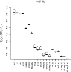
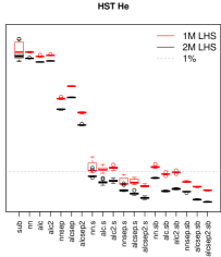
Figure 10: laGP results on the HST geometry via RMSPE calculated over 10 CV folds. Each panel is a separate experiment on a pure chemical species.

Figure 10 shows the distribution of RMSPEs obtained from our 10-fold CV on the HST data. There is a separate panel in the figure for each pure species, and the y-axis is in log space to ease inspection. First let’s focus on the results for He, shown in the bottom-middle panel of the figure. Observe that hybrid global–local modeling is essential to approach the 1% benchmark. Global or local (subset) modeling on their own are insufficient. With $N=2\times 10^{6}$ runs, random subsetting is sufficient for all local methods to consistently beat the 1% benchmark, but BLHS subsetting is better. In the smaller $N=10^{6}$ experiment, it is essential to either use a locally separable correlation structure, or BLHS pre-scaling, and using both is better still. The best comparator here is “alcsep2.sb”, i.e., using a second local design stage as recommended by Gramacy and Apley, (2015), in contrast to our earlier synthetic results which suggested deleterious effects.

The other panels in the figure, for the other five species, show a similar pattern. Besides being similar to He, the most important observation here is that the BLHS pre-scaled comparators (last six boxplots in each panel) show far lower variability than their random subsample analog (penultimate six). That the former also has lower mean than the latter is also noteworthy, but is not as striking visually.

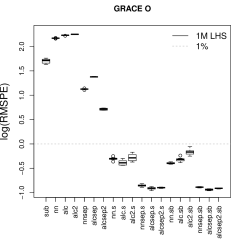
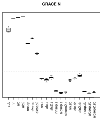
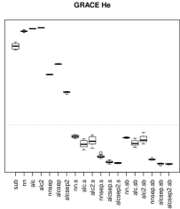
Figure 11: laGP results on the GRACE geometry via 10-fold CV; otherwise results are similar to Figure 10.

Figure 11 shows a similar suite of results for the GRACE satellite. Many of the high level observations from the HST experiment port over to this one. Perhaps the most noteworthy difference is that, despite the extra TPMC effort required for GRACE runs relative to HST ones, the ultimate emulation problem is actually easier. The RMSPEs are quite a bit lower, on the whole, compared to those in Figure 10, even with a training data set of half the size. Besides that, note that global–local modeling is essential to beat the 1% benchmark, separable local modeling is better than isotropic, and BLHS subsets offer superior accuracy. In terms of variance, BLHS and random sub-setting performs about the same in this case.

GRACE may be easier to emulate because it has a simpler, more convex geometry compared to HST. In general, the more concave an object, the more multiple reflections it will have. Besides making the mean surface more complicated, those reflections may increase the (albeit very low) noise of the TPMC simulations, making the signal harder to extract.

Figure 12: Best RMSPEs for each chemical species, zooming in on Figures 10–11.

For a finer-scale comparison we collect the best competitor (“alcsep2.sb”) from both pure-species experiments for side-by-side visualization in Figure 12, in effect zooming in on parts of Figures 10–11. In the case of He for HST, these results are from the $N=2\times 10^{6}$ experiment, like the others. Observe that, in contrast to our LANL collaborators’ prior hunch, the He species is not the hardest to predict. For HST the hardest is H. In fact, difficulty in emulation of each species appears to be monotonically increasing with molecular mass from the heaviest (O₂) to the lightest (H). An explanation may be that lighter species have higher average speed for a given atmospheric temperature, and/or larger variability in directional velocity. Hydrogen atoms, for example, will be more likely to undergo multiple collisions which the surface, complicating the input–response relationship. The results are similar for GRACE, with O₂ being an exception. Perhaps the GRACE geometry encourages reflections of O₂ particles that make O₂ have a larger number of multiple reflections from the surface than other species. Our collaborators at LANL plan to investigate further.

We close this experiment with some remarks on computational demands. Entertaining prediction on millions of testing locations in a CV format for twenty comparators is not a small task. For the prevailing $N=2\times 10^{6}$ experiments, a single species CV takes about 4500 core hours. Although substantial, this pales in comparison to the cost of TPMC simulation. The best method “alcsep2.sb” requires about 5-10% of that effort, depending on how pre-processing costs are amortized—i.e., at most 450 hours—which means that emulation is roughly two orders of magnitude faster than TPMC. Emulation runtime is also more predictable, taking less than a second per run for every single input. TPMC runs may average near ten seconds (HST) or minutes (GRACE), however the variability is quite high. Sometimes the Monte Carlo converges quickly, and sometimes it does not. Occasionally it does not converge at all. About $2$ in $10^{5}$ TPMC runs fail, and must be (randomly) restarted, which substantially increases the time required to obtain that response.

Inspired by Mehta et al., (2014b), we form a final ensemble predictor from the best pure-species predictor for HST and GRACE, respectively, following Eq. (1). To evaluate that predictor we construct a testing set via LHS in exactly the same fashion as described above (using $N=2\times 10^{6}$ for HST and $N=10^{6}$ for GRACE), except using a mixture of species rather than six separate pure ones. The mole fractions in the mixture were obtained by entering the following specification into NASA’s web-based calculator: date 1/1/2000, 0 hours, at 0 deg Latitude and Longitude, and 550 km altitude. These are:

O	O2	N	N2	He	H
0.835756795	0.000040988	0.014095898	0.005918278	0.137959854	0.006228188

The out-of-sample testing RMSPE we obtained is 0.3860 under our best comparator, “alcsep2.sb”, which was based on an average BLHS subset size of $n=1371$ using $M=3$. For HST, based on an average BLHS subset size of $n=914$ using $M=3$, the RMSPE is 0.4877 under “alcsep2.sb”. Observe that these numbers are better than the best ones in Figure 12 as the training sets were 10% larger (since they did not require CV).

6.2 Quantifying uncertainty in drags over trajectories

Here we consider a more realistic application of satellite drag emulation, via a demonstration of the value of joint modeling over a trajectory (Section 4), as opposed to a simpler pointwise approach. Four experiments are entertained. For each of HST and GRACE geometries, settings for the “free” input parameters (Table 1) are derived from a representative orbit in 2017 under periods of “quiet” (5.0) and “active” (200.0) daily geomagnetic indices.

Satellite	SMA (km)	Eccen.	Inc (deg)	AP (deg)	RAAN (deg)	TA (deg)
HST	$\ 6918$	$\ 0.00027$	$\quad 28.5$	$\quad 350$	$\quad 318$	$\quad 125$
GRACE	$\ 6713$	$\ 0.0015$	$\quad 89$	$\quad 95$	$\quad 314$	$\quad 275$

Table 5: Keplerian Orbit via SMA: Semi-Major Axis; Eccen.: Eccentricity; Inc: Inclination; AP: Argument of Perigee; RAAN: Right-Ascension of the Ascending Node; TA: True Anomaly.

Table 5 shows the Keplerian orbital elements for each satellite, which were entered into the satellite propagator program called IMPACT-PROP to determine the sequence of input settings for one full day (86,400 seconds), January 1^st, 2017, starting at 00:00:00 UTC and sampled at 10-second intervals. The result comprises of several orbits around Earth as depicted by a set of 8641 input configurations for each satellite, and each geomagnetic regime.

Figure 13: Input coordinates for GRACE-active: Umag, Ta, and alphan.

Not all parameters from Table 1 are varied by IMPACT-PROP. Figure 13 shows the nature of the orbits in the parameter space obtained for GRACE-active. Besides noting the interesting nature of the resulting trajectories, with slightly shifted circuits for each “pass” around the Earth, observe (from the axis labels) the rather limited range of values these parameters take on compared to the full range of study from Table 1. The other parameters, i.e., besides these three, were fixed near their midway values. The propagator also provides the chemical composition in LEO, which is similarly changing with the inputs, however this is less easily visualized since it is six-dimensional.

We fed those inputs and chemical compositions into the TPMC simulator to obtain a testing set of drag coefficients, with total computation times averaging about 34 hours for HST and 600 hours for GRACE, across both regimes. More precise timings are provided in Table 6. Those inputs, their corresponding chemical compositions and drag coefficients, were used as the basis of the following out-of-sample predictive experiment, mimicking the setup for our synthetic exploration in Section 4.3. Specifically, we broke the 10-second time steps into 86 sets of one hundred, contiguously, and considered each to comprise of a single trajectory through position and parameter space. Predictions under each pure chemical species (i.e., six predictions) were developed for each trajectory, separately via variations on joint and point-wise schemes, and then the species were combined via Eq. (1) using chemical compositions provided for each of the associated positions in the data.

Figure 14: Comparing log Mahalanobis distances among ALC-ex, ALC-opt, NN, ALC-pw, and NN-pw under quiet and active regimes.

The results, measuring mean and covariance accuracy simultaneously via Mahalanobis distance, are displayed in Figure 14 mimicking the format of our synthetic comparison in Figure 7. The RMSPE boxplots for each comparator were strikingly similar, so we chose not to display those in order to economize on space. It is clear from the boxplots that joint sampling dominates the pointwise alternatives, which we attribute to their ability to more accurately capture the underlying covariance structure along the trajectory. Also notice that the distances for GRACE are larger than the ones for HST, perhaps owing to the double-sized training set for the latter.

Trajectory	ALC-ex	ALC-opt	NN	ALC-pw	NN-pw	TPMC
HST-quiet	$\ 83.267$	$\ 25.047$	$\ 21.074$	$\ 89.921$	$\ 49.565$	$\ 728$
HST-active	$\ 82.014$	$\ 24.670$	$\ 20.815$	$\ 112.020$	$\ 60.356$	$\ 509$
GRACE-quiet	$\ 69.692$	$\ 12.642$	$\ 9.649$	$\ 83.952$	$\ 37.460$	$\ 12461$
GRACE-active	$\ 68.363$	$\ 12.302$	$\ 9.366$	$\ 81.356$	$\ 39.488$	$\ 13012$

Table 6: Median computation time in seconds among joint (ALC-ex, ALC-opt, NN) and pointwise (ALC-pw, and NN-pw) comparators.

Table 6 shows the median computation time for each comparator, including the actual TPMC evaluations. GRACE predictions are faster due to the smaller training data size and lower input dimension. Observe that an exhaustive ALC search is much slower than the derivative-based analogue, ALC-opt, and not much slower than the fastest method, NN. Of course, all of the predictors are orders of magnitude faster than running TPMC.

7 Discussion

In this paper we are motivated by a large-scale computer model emulation problem coming from aeronautics. Demands for accuracy in that literature require combining a large simulation effort with a high fidelity response surface. Unfortunately, those two are incompatible using current methods. Gaussian processes buckle under the weight of cubic operations, precluding training on large data. Even recent approximations, such as the laGP, which substantially increase the size capability of GPs, come up short on this task. We have proposed several extensions to laGP which, while being motivated by a particular problem, we think have the potential of broad applicability.

Our first enhancement was more technological than methodological, extending the local covariance structure to handle anisotropy while maintaining parallelizability. This required implementing a careful locking strategy with OpenMP pragmas in order to guarantee thread-safety when accessing legacy libraries. Our first methodological contribution involved a multiresolution global/local variation that fits global lengthscales from data subsets. An initial, ad hoc, approach via random data subsets worked well, but left something to be desired on a theoretical front. We were lucky to come across the work of Liu, (2014) and Liu and Hung, (2015), preferring more structured BLHS for fast consistent reproduction of global MLE of lengthscales.

When prediction is the ultimate goal, the utility of such a result is not readily apparent. Moreover, the MLE of lengthscales, whether globally or locally, need not lead to the best predictions (Zhang,, 2004). Nevertheless, we showed empirically that if the data can be pre-scaled using those estimated lengthscales, then subsequent local prediction, say via laGP, could be quite powerful indeed. This is borne out in several synthetic examples as well as on two real-world satellite drag simulators, where we demonstrate that it is possible (with GPs) to surpass a previously elusive 1% accuracy benchmark. Future work may investigate Zhang,’s insight to target elongated lengthscales, relative to the MLE, in both local and global contexts. Such analysis may help explain why a random subset outperforms BLHS in the borehole experiment summarized in the left panel of Figure 8.

A second methodological contribution comes in the form of an extension of the notion of “locale” in the laGP framework, from one location to a set of locations. We facilitate that extension with an aggregate ALC criterion and, more importantly, provide the closed form derivatives that make optimization tractable. Besides offering a more realistic application of emulation in the satellite drag application, namely, of predicting along likely trajectories in LEO, the idea offers a significant technical ability not previously enjoyed by local GP methods, that of a full predictive covariance structure, rather than simply a pointwise one. We envision several potential extensions to this framework. A natural variation may be to allow elements of the local path (or set) to be treated differentially, say by weighting. Such an extension may prove useful in modeling dynamic computer simulations via local GPs (Zhang et al.,, 2016), replacing hard clusterings with weights, say. Another would be to augment the criterion defined in Eq. (6) to include a full covariance for elements of path $W$, rather than a simple sum of variances, via Mahalanobis distances or proper scores (Eq. (25) Gneiting and Raftery,, 2007). We believe that this could be accommodated in the same framework, i.e., via analytic derivatives for library-based optimization, however we doubt that the scheme would remain computationally tractable as it would be cubic ($\mathcal{O}(|W|^{3}j^{2})$) rather than linear in $|W|$, i.e., $\mathcal{O}(|W|j^{2})$.

Finally, all methods reported in this paper have been included as additions to the laGP package for R on CRAN (Gramacy and Sun,, 2018; Gramacy,, 2016), and made available as a public Bitbucket mercurial repository: https://bitbucket.org/gramacylab/lagp. The TPMC simulation code, described in more detail in Appendix A, and all code supporting the empirical work in this paper, is available in a separate public Bitbucket mercurial repository: https://bitbucket.org/gramacylab/tpm. Our R interface to the TPMC simulator may prove valuable in the future work requiring real-world benchmarks, and supercomputer implementations without the hassle of a bespoke interface.

Acknowledgments

We are grateful to two referees for valuable comments which led to many improvements in the paper. This work was completed in part with resources provided by the University of Chicago Research Computing Center, and by facilities for Advanced Research Computing at Virginia Tech. TPMC and IMPACT-PROP were developed under the IMPACT project at Los Alamos National Laboratory. The authors would like to gratefully acknowledge funding from the National Science Foundation, awards DMS-1564438, DMS-1621722, DMS-1621746, and DMS-1739097.

Appendix A Test particle method and R interface

In the TPMC simulations presented here, particles are initialized with the appropriate Maxwellian velocity distribution based on the speed of the spacecraft and the atmospheric temperature. Particles are then randomly generated on the edges of the TPMC domain that encloses the spacecraft whose drag coefficient is being calculated. Each particle is tracked (ray-traced) until it exits the domain (in which case its tracking is completed) or until it collides with the surface. If a particle collides with the surface, the GSI model is used to appropriately re-orient the particle velocity vector and the particle is again tracked until it collides with the surface again or exits the domain. One of the primary advantages of TPMC over analytic methods when computing drag coefficients is that it can handle multiple collisions with the surface whereas analytic methods are only valid for a single collision (because they assume that the incident particles have a Maxwellian velocity distribution which is no longer true for particles that have already reflected off the spacecraft surface).

The supplementary material contains a version of the original TPMC C code, developed at Los Alamos National Laboratory, which we have modified to utilize OpenMP for efficient symmetric multiprocessor parallelization (i.e., utilization of multiple cores within a node). A wrapper to that C library, written in R, allows easy access to new simulations from within R. Everything is provided via a public Bitbucket mercurial repository: https://bitbucket.org/gramacylab/tpm. The package is not a CRAN package, but it is structured in a very similar way. After cloning the repository, there are two steps required to perform new TPMC simulations. First, to compile the C library, change into tpm/src and execute

% R CMD SHLIB -o tpm.so *.c

Then, the second step involves sourcing wrapper files from within R.

R> source("tpm/R/tpm.R")

Now we are ready to run our first TPMC simulations. Below is code building a data frame of eight uniformly random settings of the free parameters in Table 1, repeated twice for sixteen settings total.

R> n <- 8
R> X <- data.frame(Umag=runif(n, 5500, 9500), Ts=runif(n, 100, 500),
+    Ta=runif(n, 200, 2000), theta=runif(n,-pi,pi), phi=runif(n,-pi/2,pi/2),
+    alphan=runif(n), sigmat=runif(n))
R> X <- rbind(X,X)

Next we need to specify a mesh file. The directory tpm/Mesh_Files contains all of the meshes used in this paper, and several others including the ones for the International Space Station (ISS). Below we specify the GRACE mesh.

R> mesh <- "tpm/Mesh_Files/GRACE_A0_B0_ascii_redone.stl"

Then specify the mixture vector over the chemical species, e.g., pure He.

R> moles <- c(0,0,0,0,1,0)

With those inputs, a blocked TPMC batch may be invoked as follows.

R> system.time(y <- tpm(X, moles=moles, stl=mesh, verb=0))

##   user     system  elapsed
## 3204.680    1.136  265.502

The elapsed time is 266 seconds (30 minutes), cumulative, for the sixteen evaluations. That is an average of seventeen seconds per evaluation. However, by inspecting the “user” time we can see that the execution was parallelized. The desktop this was performed on is an 8-core 64-bit Intel i7-6900K CPU at 3.20 GHz. The cores are hyperthreaded, meaning that it can often perform sixteen numerical tasks in parallel rather than the usual eight. However, the speedup is not 16-fold since some of the inputs take longer than others. Instead we observed about a 12-fold speedup, amortized over all sixteen runs. On a single core machine, the execution time would have been about 53 minutes, or about 3.3 minutes per simulation.

The replication in the design can give us an indication of the level of noise in these Monte Carlo simulations.

R> mean((y[1:n] - y[(n+1):length(y)])^2)

## [1] 4.120074e-05

So the noise is higher than machine precision, but low relative to the range of y-values.

R> range(y)

## [1] 1.812294 3.419442

The R wrapper routines contain a tpm.parallel command that allows further cluster-style parallelization through the built-in R library. It works similarly to tpm, taking a cluster object created by the makeCluster command, establishing socket or MPI connections to computer nodes. The tpm.parallel command was used on University of Chicago’s Research Computer Center’s midway cluster to perform TPMC evaluations used for training and testing of HST and GRACE satellite predictors in Section 6. Our supplementary material includes the data files from those runs, along with the smaller runs compiled by Mehta et al., (2014b) using the earlier stand-alone C version of the TPMC library.

To independently verify the accuracy results reported by Mehta et al., (2014b) we offer the following code re-creating their test for GRACE in pure He. First, read in the data.

R> train <- read.table("satdrag/GRACE/CD_GRACE_1000_He.dat")
R> test <- read.table("satdrag/GRACE/CD_GRACE_100_He.dat")
R> nms <- c("Umag", "Ts", "Ta", "alphan", "sigmat", "theta", "phi", "drag")
R> names(train) <- names(test) <- nms
R> print(r <- apply(rbind(train, test)[,-8], 2, range))

##          Umag       Ts        Ta       alphan       sigmat        theta
## [1,] 5501.933 100.0163  201.2232 0.0008822413 0.0007614135 1.270032e-05
## [2,] 9497.882 499.8410 1999.9990 0.9999078000 0.9997902000 6.978310e-02
##              phi
## [1,] -0.06978125
## [2,]  0.06971254

The output above allows us to compare ranges of inputs against Tables 1–2. Next, code those inputs in the unit cube as follows.

R> X <- train[,1:7]; XX <- test[,1:7]
R> for(j in 1:ncol(X)){
+      X[,j] <- X[,j] - r[1,j]; XX[,j] <- XX[,j] - r[1,j];
+      X[,j] <- X[,j]/(r[2,j]-r[1,j]); XX[,j] <- XX[,j]/(r[2,j]-r[1,j])
+  }

Finally, we are ready to fit a GP. The code below uses the (non-approximate) separable covariance GP capability built into the laGP package.

R> library(laGP)
R> fit.gp <- newGPsep(X, train[,8], 2, 1e-6, dK=TRUE)
R> mle <- mleGPsep(fit.gp)
R> p <- predGPsep(fit.gp, XX, lite=TRUE)
R> rmspe <- sqrt(mean((100*(p$mean - test[,8])/test[,8])^2))
R> rmspe

## [1] 0.7401575

The final calculation is RMSPE, and observe that this is below the desired 1% benchmark. Similar results are obtained with the other species, whose data files are also provided in the supplementary material.

Appendix B Compactly supported covariances v. laGP

Here we follow an example provided by the CSC authors, Kaufman et al., (2012):

https://www.stat.berkeley.edu/~cgk/rcode/assets/SparseEmExample.R

Below is an implementation of the borehole function (Section 5), followed by a random partition into training and testing sets via a joint LHS. This is almost verbatim from the code linked above, but we re-create it here in order to add our own laGP-based comparisons.

R> borehole <- function(x){
+    rw <- x[1] * (0.15 - 0.05) + 0.05
+    r <-  x[2] * (50000 - 100) + 100
+    Tu <- x[3] * (115600 - 63070) + 63070
+    Hu <- x[4] * (1110 - 990) + 990
+    Tl <- x[5] * (116 - 63.1) + 63.1
+    Hl <- x[6] * (820 - 700) + 700
+    L <-  x[7] * (1680 - 1120) + 1120
+    Kw <- x[8] * (12045 - 9855) + 9855
+    m1 <- 2 * pi * Tu * (Hu - Hl)
+    m2 <- log(r / rw)
+    m3 <- 1 + 2*L*Tu/(m2*rw^2*Kw) + Tu/Tl
+    return(m1/m2/m3)
}

## Training-testing partition
R> n <- 4000
R> npred <- 500
R> dim <- 8
R> library(lhs)
R> x <- randomLHS(n+npred, dim)
R> y <- apply(x, 1, borehole)
R> ypred.0 <- y[-(1:n)]; y <- y[1:n]
R> xpred <- x[-(1:n),]; x <- x[1:n,]

Then comes the fitting functions, which are partitioned into routines that find the desired level of sparsity, which for this example is 99%, followed by sampling from the posterior at that level, and then gathering predictions after burn-in.

R> mc <- find.tau(den=1-0.99, dim=ncol(x)) * ncol(x)
R> time1 <- system.time(
+    tau <- mcmc.sparse(y, x, mc=mc, degree=2, maxint=2, B=2000, verbose=F))
R> index <- seq(500+1, 2000, by=10)
R> time2 <- system.time(ypred.sparse <-
+    pred.sparse(tau[index,], x, y, xpred, degree=2, maxint=2,verbose=F))

Here is a similar code for a 99.9% sparse version.

R> mc <- find.tau(den=1-0.999, dim=ncol(x)) * ncol(x)
R> time5 <- system.time(
+    tau <- mcmc.sparse(y, x, mc=mc, degree=2, maxint=2, B=2000, verbose=F))
R> index <- seq(500+1, 2000, by=10)
R> time6 <- system.time(ypred.sparse <-
+    pred.sparse(tau[index,], x, y, xpred, degree=2, maxint=2, verbose=F))

For a fair comparison, Kaufman et al., (2012) provide a non-sparse alternative.

R> time3 <- system.time(phi <- mcmc.nonsparse(y, x, B=200, verbose=F))
R> index <- seq(50+1, 200, by=10)
R> time4 <- system.time(ypred.nonsparse <-
+    pred.nonsparse(phi[index,], x, y, xpred, 2, verbose=F))

Here is how these comparators fare in terms of computation time: about a factor of 3 speed-up by being 99% sparse, and 10$\times$ better than that with 99.9% sparsity.

R> times <- c(sparse=as.numeric(time1[3]+time2[3]),
+    dense=10*as.numeric(time3[3]+time4[3]),
+    s999=as.numeric(time5[3]+time6[3]))
R> times

##   sparse   dense     s999
##  3409.157 9020.870  258.196

The proper scores (Eq. (27) Gneiting and Raftery,, 2007), with larger being better, follow a predictable pattern: the more dense the higher the accuracy.

R> s2s <- ypred.sparse$var
R> s2n <- ypred.nonsparse$var
R> s29 <- ypred.sparse$var
R> scores <- c(sparse=mean(- (ypred.sparse$mean - ypred.0)^2/s2s - log(s2s)),
+   dense=mean(-(ypred.nonsparse$mean - ypred.0)^2/s2n - log(s2n)),
+   s999=mean(-(ypred.sparse$mean - ypred.0)^2/s29 - log(s29)))
R> scores

##   sparse    dense     s999
## -1.616263 -2.636446 -1.796645

Now what about laGP? The two commands below derive predictions based on an isotropic and separable Gaussian correlation structure, respectively.

R> out <- aGP(x, y, xpred, d=list(max=20), omp.threads=8, verb=0)
R> outs <- aGPsep(x, y, xpred, d=list(max=20), omp.threads=8, verb=0)

In terms of time, laGP is more than an order of magnitude faster than even the sparsest CSC version.

R> times <- c(times, aGP=as.numeric(out$time), aGPs=as.numeric(outs$time)))
R> times

##  sparse     dense     s999       aGP      aGPs
## 3409.157   9020.870  258.196    9.059    8.929

Not only are they faster, but also they are (much) more accurate, especially the separable version.

R> s2 <- out$var; s2s <- outs$var
R> scores <- c(scores, aGP=mean(-(out1$mean - ypred.0)^2/s2 - log(s2)),
+    aGPs=mean(-(out1$mean - ypred.0)^2/s2s - log(s2s))))
R> scores

##   sparse       dense          s999         aGP         aGPs
## -1.6162629   -2.6364460   -1.7966449   -0.6024819   0.1057021

Finally, as a demonstration of the potential of multiresolution modeling, consider a single random subset with 1000 points fit with full-GP subroutines in the laGP package.

R> da <- darg(list(mle=TRUE, max=100), x)
R> subs <- sample(1:nrow(x), 1000, replace=FALSE)
R> gpsi <- newGPsep(x[subs,], y[subs], rep(da$start, dim), g=1e-3, dK=TRUE)
R> that <- mleGPsep(gpsi, tmin=d2$min, tmax=d2$max, ab=d2$ab, maxit=200)
R> psub <- predGPsep(gpsi, xpred, lite=TRUE)
R> deleteGPsep(gpsi)

Then we can scale the predictors by the square root of estimated lengthscales and fit another isotropic local approximate GP, initialized at a lengthscale of 1.

R> scale <- sqrt(that$d)
R> xs <- x; xpreds <- xpred
R> for(j in 1:ncol(xs)){
+      xs[,j] <- xs[,j] / scale[j]
+      xpreds[,j] <- xpreds[,j] / scale[j]
+  }
R> outmr <- aGP(xs, y, xpreds, d=list(start=1, max=20), omp.threads=8,
+  verb=0)

The new multiresolution predictor is the best of all, but notice that the subset GP is also very good. Apparently the compactly supported covariance structure, which generated our dense results above, does not offer enough smoothness for the borehole data.

R> s2sub <- out3$var; s2mr <- out4$var
R> scores <- c(scores, sub=mean(-(psub$mean-ypred.0)^2/s2sub - log(s2sub)),
+    aGPmr=mean(-(out3$mean - ypred.0)^2/s2mr - log(s2mr)))
R> scores

##   sparse      dense       s999        aGP       aGP2        aGPs
## -1.6162629  -2.6364460 -1.7966449 -0.6024819 -0.5693178  0.1057021
##     sub       aGPsm
##  0.7415339  1.1909690

Further improvements (scores above 5) are possible with aGPsep with a smaller nugget value than the default, e.g., g=1/10000000, but we leave those extensions to the curious reader.

Appendix C Derivative derivation (separable GP version)

Here we derive the expression behind the components of the gradient of the “joint” ALC defined in Eq. (7) from Section 4.2. We allow any form of the correlation function where derivatives may be calculated relative to the spatial locations, $x$. Following Eq. (7), we take the derivative with respect to each coordinate of $x_{j+1}$. For $\ell=1,\dots,p$,

$$\frac{\partial}{\partial(x_{j+1})_{\ell}} \left\{v_{j}(W)-v_{j+1}(W)\right\}=\frac{\partial}{\partial(x_{j+1})_{\ell}}\left\{\frac{1}{|W|}\sum_{w\in W}\left[v_{j}(w)-v_{j+1}(w)\right]\right\}$$

$$=\frac{1}{|W|}\sum_{w\in W}\frac{\partial}{\partial(x_{j+1})_{\ell}}\Big{\{}k_{j}^{\top}(w)G_{j}(x_{j+1})v_{j}(x_{j+1})k_{j}(w)$$

$$\quad\quad\quad\quad\quad\quad\quad\quad\quad\quad+2k_{j}^{\top}(w)g_{j}(x_{j+1})K(x_{j+1},w)+K(x_{j+1},w)^{2}/v_{j}(x_{j+1})\Big{\}},$$

where

$$\frac{\partial}{\partial(x_{j+1})_{\ell}}\left\{k_{j}^{\top}(w)G_{j}(x_{j+1})v_{j}(x_{j+1})k_{j}(w)+2k_{j}^{\top}(w)g_{j}(x_{j+1})K(x_{j+1},w)+\frac{K(x_{j+1},w)^{2}}{v_{j}(x_{j+1})}\right\}$$ (8)

$$=k_{j}^{\top}(w)\left\{\left[\frac{\partial}{\partial(x_{j+1})_{\ell}}G_{j}(x_{j+1})\right]v_{j}(x_{j+1})+G_{j}(x_{j+1})\left[\frac{\partial}{\partial(x_{j+1})_{\ell}}v_{j}(x_{j+1})\right]\right\}k_{j}(w)$$

$$\quad+2k_{j}^{\top}(w)\left\{\left[\frac{\partial}{\partial(x_{j+1})_{\ell}}g_{j}(x_{j+1})\right]K(x_{j+1},w)+g_{j}(x_{j+1})\left[\frac{\partial}{\partial(x_{j+1})_{\ell}}K(x_{j+1},w)\right]\right\}$$

$$\quad+2K(x_{j+1},w)\left[\frac{\partial}{\partial(x_{j+1})_{\ell}}K(x_{j+1},w)\right]v_{j}^{-1}(x_{j+1})+K(x_{j+1},w)^{2}\left[\frac{\partial}{\partial(x_{j+1})_{\ell}}v_{j}^{-1}(x_{j+1})\right].$$

Particularly,

$$\frac{\partial}{\partial(x_{j+1})_{\ell}}G_{j}(x_{j+1}) =2\left[\frac{\partial}{\partial(x_{j+1})_{\ell}}g_{j}(x_{j+1})\right]g^{\top}_{j}(x_{j+1}),$$ (9)

$$\frac{\partial}{\partial(x_{j+1})_{\ell}}g_{j}(x_{j+1}) =-K^{-1}_{j}\left\{\!\left[\frac{\partial}{\partial(x_{j+1})_{\ell}}k_{j}(x_{j+1})\right]v_{j}^{-1}(x_{j+1})+k_{j}(x_{j+1})\left[\frac{\partial}{\partial(x_{j+1})_{\ell}}v_{j}^{-1}(x_{j+1})\right]\!\right\},$$

$$\frac{\partial}{\partial(x_{j+1})_{\ell}}v_{j}(x_{j+1}) =2\left[\frac{\partial}{\partial(x_{j+1})_{\ell}}k^{\top}_{j}(x_{j+1})K_{j}^{-1}k_{j}(x_{j+1})\right].$$ (10)

By plugging Eqs. (9–10), Eq. (8) can be reorganized as follows:

$$\mbox{Eq.~{}(\ref{eq:dds1})}= -k^{\top}_{j}(w)K_{J}^{-1}\left[\dot{k}_{\ell}+k_{j}(x_{j+1})av_{j}^{-1}(x_{j+1})\right]g_{j}^{\top}(x_{j+1})k_{j}(w)$$

$$-k^{\top}_{j}(w)g_{j}(x_{j+1})\!\left[\dot{k}^{\top}_{\ell}K_{J}^{-1}+k_{j}^{\top}(x_{j+1})K_{J}^{-1}av_{j}^{-1}(x_{j+1})\right]\!k_{j}(w)$$

$$-k_{j}^{\top}(w)g_{j}(x_{j+1})g_{j}^{\top}(x_{j+1})ak_{j}(w)$$

$$+2k_{j}^{\top}(w)\left\{-K_{J}^{-1}\left[\dot{k}_{\ell}+k_{j}(x_{j+1})av_{j}^{-1}(x_{j+1})\right]v_{j}^{-1}(x_{j+1})K(x_{j+1},w)+g_{j}(x_{j+1})\dot{K}_{\ell}\right\}$$

$$+K(x_{j+1},w)\left[2\dot{K}_{\ell}+K(x_{j+1},w)av_{j}^{-1}(x_{j+1})\right]v_{j}^{-1}(x_{j+1}),$$

where the macros $\dot{k}_{\ell}$ (a $j$-vector), $\dot{K}_{\ell}$ and $a$ (both scalars) are

$$\dot{k}_{\ell}=\frac{\partial}{\partial(x_{j+1})_{\ell}}k_{j}(x_{j+1})=\left\{-\frac{2\left[(x_{j+1})_{\ell}-(x_{j})_{\ell}\right]}{\theta_{\ell}}\exp\left\{-\sum_{\ell=1}^{p}\frac{\left[(x_{j+1})_{\ell}-(x_{j})_{\ell}\right]^{2}}{\theta_{\ell}}\right\}\right\}_{j\times 1},$$

$$\text{where $x_{j}$ is any location within the current local design}.$$

$$\dot{K}_{\ell}=\frac{\partial}{\partial(x_{j+1})_{\ell}}K(x_{j+1},w)=-\frac{2\left[(x_{j+1})_{\ell}-w_{\ell}\right]}{\theta_{\ell}}\exp\left\{-\sum_{\ell=1}^{p}\frac{\left[(x_{j+1})_{\ell}-w_{\ell}\right]^{2}}{\theta_{\ell}}\right\},$$

$$a=2\frac{\partial k_{j}^{\top}(x_{j+1})}{\partial(x_{j+1})_{\ell}}K_{j}^{-1}k_{j}(x_{j+1}).$$

Eq. (8) can be further simplified to

$$-2k^{\top}_{j}(w)K^{-1}_{J}\left[\frac{\partial k_{j}(x_{j+1})}{\partial(x_{j+1})_{\ell}}+\frac{k_{j}(x_{j+1})a}{v_{j}(x_{j+1})}\right]b-abc+2c\frac{\partial K(x_{j+1},w)}{\partial(x_{j+1})_{\ell}}$$

where the macros $b$ and $c$ (both scalars) are

$$b=g_{j}^{\top}(x_{j+1})k_{j}(w)-K(x_{j+1},w)/v_{j}(x_{j+1}),\quad\mbox{and}\quad c=g_{j}^{\top}(x_{j+1})k_{j}(w)+K(x_{j+1},w)/v_{j}(x_{j+1}).$$

The final expression for the components of the gradient of the “joint” ALC is as follows:

$$\frac{\partial}{\partial(x_{j+1})_{\ell}} \left\{v_{j}(W)-v_{j+1}(W)\right\}$$

$$= \frac{1}{|W|}\sum_{w\in W}\left\{-2k^{\top}_{j}(w)K^{-1}_{J}\left[\frac{\partial k_{j}(x_{j+1})}{\partial(x_{j+1})_{\ell}}+\frac{k_{j}(x_{j+1})a}{v_{j}(x_{j+1})}\right]b-abc+2c\frac{\partial K(x_{j+1},w)}{\partial(x_{j+1})_{\ell}}\right\}.$$

Appendix D 2d representative predictive paths

Figure 15 shows a representative plot of 2d predictive paths generated randomly as follows.

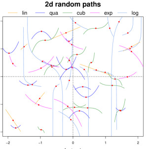
Figure 15: A representative plot of 2d predictive paths

First, a line type (linear, quadratic, cubic, exponential, and natural logarithm) is chosen uniformly at random. The line is then drawn, via a collection of discrete points, from the origin via specifications (e.g., resolution and length) provided by the user. The discrete set of coordinates is then shifted and scaled, uniformly at random, into a specified 2d rectangle ($[-2,2]^{2}$ in the figure) with the restriction that at least half of the points comprising the line lie within the rectangle. A centering dot (mostly for visual effect) is calculated as the midway point on the discrete set of points making up the line.

Appendix E laGP versus others

A referee suggested we compare laGP with some other methods, and provided the beginnings of a script that applied RobustGaSP (Gu et al.,, 2018) and DiceKriging (Roustant et al.,, 2012) on a small ($N=400$) borehole example (Section 5.1). We augmented that script to include laGP’s full GP capability as a comparator. The full GP functionality in laGP is bare-bones: simple MLE calculations via (2) for unknown lengthscale hyperparameters. This is extended to global MLEs of lengthscale from large data sets via BLHS, subsequent local sub-design and local MLE estimation as explained in the main body of our manuscript, and detailed by Gramacy and Apley, (2015). Once the local design has been determined, inference for hyperparameters is fundamentally not different than in the full GP case—just with less data. Gu et al.,’s careful approach to GP inference is impressive in small-$N$ contexts, and Roustant et al.,’s “DICE”-family of methods is extensive in terms of the breadth of modeling options. Yet, as we summarize below, laGP methods are competitive. Of course, the local approximation laGP provides is unmatched when it comes to data size. Neither of these packages can handle data an order of magnitude larger than the $N=400$ in this small study, let alone the two-to-three magnitudes larger which are the target of this manuscript. We augmented the script provided by the referee, which is very similar to the one summarized by Figure 8, to include laGP-based comparators, and wrapped it in a for loop to obtain thirty repetitions, and include it along with our supplementary material.

Figure 16: Comparisons between RobustGaSP, DiceKriging, and laGP-based methods including full and local variations on an $N=400$-sized borehole example. Left: empirical distribution of log RMSEs. Right: empirical distribution of computational cost via wall-clock time (in seconds). Comparators “local-100K” and “local-1M” correspond to the “alc.sb” comparators from Figure 8 and are based on the multifidelity framework of Section 3.

The results of that experiment are provided in Figure 16. The left panel shows out-of-sample RMSE in log space, and the right panel collects execution time. The first four boxplots, from left to right in either panel, correspond to full GPs fit to $N=400$ training sites. RobustGaSP is the best here, but it is also thirty times slower than the second best, via the full GP functionality in laGP. The local modeling features of laGP are competitive on this small example, but not better than full GP modeling. When the data are small enough for full GP modeling, local approximations are neither necessary nor beneficial. However, when the data are bigger they are indeed quite necessary, and they represent an efficient way to leverage the information available in such samples, beating the RobustGaSP comparator. Note that the runtime for laGP in these larger $N$ settings is nearly identical to the smaller $N$ since both use a local neighborhood size of $n=50$. The only difference is an $N\log N$ pre-processing step to which is nearly instantaneous even with large $N$.

It is possible that the ideas behind RobustGaSP could be ported over to the local setting, however, it is not immediately obvious how to do that (from an implementation perspective) at this time. Clearly the requisite order of magnitude larger runtime will limit the size of problems on which such an approach can be applied.

References

- Achenbach, (2009) Achenbach, J. (2009). “Debris from Satellites’ Collision said to Pose Small Risk to Space Station.” The Washington Post.
- Bastos and O’Hagan, (2009) Bastos, L. and O’Hagan, A. (2009). “Diagnostics for Gaussian Process Emulators.” Technometrics, 51, 4, 425–438.
- Berger et al., (2001) Berger, J., De Oliveira, V., and Sanso, B. (2001). “Objective Bayesian Analysis of Spatially Correlated Data.” Journal of the American Statistical Association, 96, 1361–1374.
- Byrd et al., (1995) Byrd, R., Qiu, P., Nocedal, J., , and Zhu, C. (1995). “A Limited Memory Algorithm for Bound Constrained Optimization.” Journal on Scientific Computing, 16, 5, 1190–1208.
- Cercignani and Lampis, (1971) Cercignani, C. and Lampis, M. (1971). “Kinetic Models for Gas-Surface Interactions.” Transport Theory and Statistical Physics, 1, 2, 101–114.
- Cohn, (1996) Cohn, D. A. (1996). “Neural Network Exploration using Optimal Experimental Design.” In Advances in Neural Information Processing Systems, vol. 6(9), 679–686. Morgan Kaufmann Publishers.
- Cressie, (1991) Cressie, N. (1991). Statistics for Spatial Data, revised edition. John Wiley and Sons, Inc.
- Gneiting and Raftery, (2007) Gneiting, T. and Raftery, A. (2007). “Strictly Proper Scoring Rules, Prediction, and Estimation.” Journal of the American Statistical Association, 102, 477, 359–378.
- Gramacy, (2016) Gramacy, R. (2016). “laGP: Large-Scale Spatial Modeling via Local Approximate Gaussian Processes in R.” Journal of Statistical Software, 72, 1, 1–46.
- Gramacy and Apley, (2015) Gramacy, R. and Apley, D. (2015). “Local Gaussian Process Approximation for Large Computer Experiments.” Journal of Computational and Graphical Statistics, 24, 2, 561–578. See arXiv:1303.0383.
- Gramacy and Haaland, (2015) Gramacy, R. and Haaland, B. (2015). “Speeding Up Neighborhood Search in Local Gaussian Process Prediction.” Technometrics, to appear. ArXiv:1409.0074.
- Gramacy et al., (2014) Gramacy, R., Niemi, J., and Weiss, R. (2014). “Massively Parallel Approximate Gaussian Process Regression.” Journal of Uncertainty Quantification, 2, 1, 564–584.
- Gramacy and Sun, (2018) Gramacy, R. B. and Sun, F. (2018). laGP: Local Approximate Gaussian Process Regression. R package version 1.5-2.
- Gu and Berger, (2016) Gu, M. and Berger, J. (2016). “Parallel Partial Gaussian Process Emulation for Computer Models with Massive Output.” Annals of Applied Statistics, 10, 3, 1317–1347.
- Gu et al., (2018) Gu, M., Wang, X., and Berger, J. (2018). “Robust Gaussian Stochastic Process Emulation.” Annals of Statistics, 46, 3038–3066.
- Kaufman et al., (2012) Kaufman, C., Bingham, D., Habib, S., Heitmann, K., and Frieman, J. (2012). “Efficient Emulators of Computer Experiments using Compactly Supported Correlation Functions, with An Application to Cosmology.” The Annals of Applied Statistics, 5, 4, 2470–2492.
- Kessler and Cour‐Palais, (1978) Kessler, D. and Cour‐Palais, B. (1978). “Collision Frequency of Artificial Satellites: The Creation of A Debris Belt.” JCR Space Physics, 83, 2637–2646.
- Lawrence et al., (2014) Lawrence, E., Higdon, D., Walker, A., and Shoemaker, M. (2014). “Estimation for Satellite Collision Probabilities using Importance Sampling.” Proceedings of the 24th AAS/AIAA Space Flight Mechanics Meeting.
- Liu, (2014) Liu, Y. (2014). “Recent Advances in Computer Experiment Modeling.” Tech. rep., Rutgers, The State University of New Jersey, New Brunswick, New Jersey.
- Liu and Hung, (2015) Liu, Y. and Hung, Y. (2015). “Latin Hypercube Design-based Block Bootstrap for Computer Experiment Modeling.” Tech. rep., Rutgers, The State University of New Jersey, New Brunswick, New Jersey.
- Mehta et al., (2014a) Mehta, P., Walker, A., McLaughlin, C., and Koller, J. (2014a). “Comparing Physical Drag Coefficients Computed using Different Gas-surface Interaction Models.” Journal of Spacecraft and Rockets, 51, 3, 873–883.
- Mehta et al., (2014b) Mehta, P. M., Walker, A., Lawrence, E., Linares, R., Higdon, D., and Koller, J. (2014b). “Modeling Satellite Drag Coefficients with Response Surfaces.” Advances in Space Research, 54, 8, 1590–1607.
- Molga and C., (2005) Molga, M. and C., S. (2005). “Test Functions for Optimization Needs.”
- Morris et al., (1993) Morris, D., Mitchell, T., and Ylvisaker, D. (1993). “Bayesian Design and Analysis of Computer Experiments: Use of Derivatives in Surface Prediction.” Technometrics, 35, 243–255.
- Picone et al., (2002) Picone, J., Hedin, A., Drob, D. P., and Aikin, A. (2002). “NRLMSISE-00 Empirical Model of the Atmosphere: Statistical Comparisons and Scientific Issues.” Journal of Geophysical Research: Space Physics, 107, A12.
- R Core Team, (2017) R Core Team (2017). R: A Language and Environment for Statistical Computing. R Foundation for Statistical Computing, Vienna, Austria.
- Roustant et al., (2012) Roustant, O., Ginsbourger, D., and Deville, Y. (2012). “DiceKriging, DiceOptim: Two R Packages for the Analysis of Computer Experiments by Kriging-based Metamodeling and Optimization.” Journal of Statistical Software, 51, 1, 1–55.
- Sacks et al., (1989) Sacks, J., Welch, W. J., Mitchell, T. J., and Wynn, H. P. (1989). “Design and Analysis of Computer Experiments.” Statistical Science, 4, 409–435.
- Sang and Huang, (2012) Sang, H. and Huang, J. Z. (2012). “A Full Scale Approximation of Covariance Functions for Large Spatial Data Sets.” Journal of the Royal Statistical Society: Series B, 74, 1, 111–132.
- Santner et al., (2003) Santner, T. J., Williams, B. J., and Notz, W. I. (2003). The Design and Analysis of Computer Experiments. New York, NY: Springer-Verlag.
- Seo et al., (2000) Seo, S., Wallat, M., Graepel, T., and Obermayer, K. (2000). “Gaussian Process Regression: Active Data Selection and Test Point Rejection.” In Proceedings of the International Joint Conference on Neural Networks, vol. III, 241–246. IEEE.
- Stein, (1999) Stein, M. L. (1999). Interpolation of Spatial Data. New York, NY: Springer.
- Surjanovic and Bingham, (2014) Surjanovic, S. and Bingham, D. (2014). “Virtual Library of Simulation Experiments: Test Functions and Datasets.” Retrieved December 4, 2014, from http://www.sfu.ca/~ssurjano.
- Varin et al., (2011) Varin, C., Reid, N., and Firth, D. (2011). “An Overview of Composite Likelihood Methods.” Statistica Sinica, 21, 1, 5–42.
- Zhang et al., (2015) Zhang, B., Konomi, B., Sang, H., Karagiannis, G., and Lin, G. (2015). “Full Scale Multi-output Gaussian Process Emulator with Nonseparable Auto-covariance Functions.” Jounal of Computational Physics, 300, 623–642.
- Zhang, (2004) Zhang, H. (2004). “Inconsistent Estimation and Asymptotically Equal Interpolations in Model-based Geostatistics.” Journal of the American Statistical Association, 99, 465, 250–261.
- Zhang et al., (2016) Zhang, R., Lin, C., and Ranjan, P. (2016). “Local Gaussian Process Model for Large-Scale Dynamic Computer Experiments.” Tech. rep., Queens University, Kingston, Ontario, Canada.