Gauged merons

Abstract

We construct new class of regular soliton solutions of the gauged planar Skyrme model on the target space $S^{2}$ with fractional topological charges in the scalar sector. These field configurations represent Skyrmed vortices, they have finite energy and carry topologically quantized magnetic flux $\Phi=2\pi n$ where $n$ is an integer. Using a special version of the product ansatz as guide, we obtain by numerical relaxation various multimeron solutions and investigate the pattern of interaction between the fractionally charged solitons. We show that, unlike the vortices in the Abelian Higgs model, the gauged merons may combine short range repulsion and long range attraction. Considering the strong gauge coupling limit we demonstrate that the topological quantization of the magnetic flux is determined by the Poincaré index of the planar components $\phi_{\perp}=\phi_{1}+i\phi_{2}$ of the Skyrme field.

Introduction.   The past two decades have seen remarkable progress in our understanding of various soliton solutions in non-linear systems. These spatially localized field configurations arise in many different areas of physics, e.g., physics of condensed matter Solitons ; Ackerman:2017lse , solid state physics Kosevich , non-linear optics Mollenauer , biophysics Dauxois , field theory MantonSutcliffe , cosmology Vilenkin and other disciplines. Further, this development has sparked a lot of interest in the mathematical investigation of non-linear systems, the fascinating techniques developed in this area of modern theoretical physics, find many other applications.

An interesting example of the model, which admits soliton solutions, is non-linear $O(3)$ sigma model, which is also known as the baby Skyrme model. It can be considered as a planar analogue of a $\left(3+1\right)$ dimensional Skyrme theory Skyrme:1961vq . The baby Skyrme model attracts a special attention since this simple theory finds various direct physical realizations. It was formulated originally as a modification of the Heisenberg model of interacting spins Bogolubskaya:1989ha . Further, hexagonal lattices of two-dimensional skyrmions were observed in a thin ferromagnetic layer Yu , and in a metallic itinerant-electron magnet, where the Skyrmion lattice was detected by results of neutron scattering Muhlenbauer . The Skyrmions naturally arise in various condensed matter systems with intrinsic and induced chirality, some modification of the baby Skyrme model with the Dzyaloshinskii-Moriya interaction term was suggested to model noncentrosymmetric ferromagnetic planar structures Bogdanov . Very recently there has been a new trend in material science, here two dimensional magnetic Skyrmions were discussed in the context of future applications in development of data storage technologies and emerging spintronics, see e.g. Heinze ; Liu . The planar Skyrmions are also known through a specific contribution to the topological quantum Hall effect Neubauer . In this framework the Skyrmion-like states are coupled to fluxes of magnetic field, they effectively represent solutions of the Skyrme-Maxwell theory.

The planar Skyrme-Maxwell model was considered for the first time in Gladikowski:1995sc . Recently, there has been renewed interest in this model related with construction of multisoliton solutions Samoilenka:2015bsf and investigation of the solutions of the Bogomolny type equation for the gauged planar Skyrme model Adam:2012pm ; Adam:2017ahh . The effect of a Chern-Simons term on the stricture of the solutions of this model was studied in Navarro-Lerida:2016omj ; Samoilenka:2016wys . An important observation is that the magnetic flux of the solutions is not in general quantized, there is no topological number, associated with the gauge sector of the model. However, in the strong gauge coupling limit, the magnetic flux becomes quantized.

Interestingly, besides Skyrmions the non-linear $O(3)$ sigma model supports solutions of a different type, the merons Gross:1977wu . They carry topological charge one half, however the merons are singular solutions, an isolated meron has infinite energy.

The aim of the present paper is to revisit the solutions of the planar Skyrme-Maxwell theory. We introduce a new class of regular localized soliton solutions with finite energy, the gauged merons which are carrying topologically quantized magnetic flux, and possess a fractional topological charges in the scalar sector. Although these solutions resemble the vortices in the Abelian Higgs model, they properties are different, in particular the effective potential of interaction between the gauded merons may combine a short-range repulsion and a long-range dipole attraction.

The model.  We consider the gauged planar non-linear $O(3)$ sigma model in $(2+1)$ dim, defined by the Lagrangian density

$$L=-\frac{1}{4g^{2}}F_{\mu\nu}F^{\mu\nu}+\frac{1}{2}D_{\mu}\vec{\phi}\cdot D^{\mu}\vec{\phi}-\frac{1}{4}(D_{\mu}\vec{\phi}\times D_{\nu}\vec{\phi})^{2}-V(\vec{\phi})\,,$$ (1)

where the triplet of scalar fields $\vec{\phi}=(\phi_{1},\phi_{2},\phi_{3})$ is constrained as $\vec{\phi}\cdot\vec{\phi}=1$ and $g$ is the gauge coupling. We introduced the usual Maxwell term with the field strength tensor defined as $F_{\mu\nu}=\partial_{\mu}A_{\nu}-\partial_{\nu}A_{\mu}$. The coupling of the Skyrme field to the magnetic field is given by the covariant derivative Adam:2012pm ; Schroers:1995he ; Gladikowski:1995sc

$$D_{\mu}\vec{\phi}=\partial_{\mu}\vec{\phi}+A_{\mu}\vec{\phi}\times\vec{n}\,\qquad\vec{n}=(0,0,1)\,.$$

Note that the potential breaks the original $O(3)$ symmetry of the sigma model to $O(2)$, the Lagrangian (1) is invariant under the local $U(1)$ transformations

$$\phi_{\perp}\rightarrow e^{i\alpha}\phi_{\perp}\,,\quad A_{\mu}\rightarrow A_{\mu}+\partial_{\mu}\alpha_{\mu}\,,$$ (2)

where $\phi_{\perp}=\phi_{1}+i\phi_{2}$. Henceforth we consider only static configurations with $A_{0}=0$, with magnetic field $B=\partial_{1}A_{2}-\partial_{2}A_{1}$.

In 2+1 dimensions the presence of the potential term $V(\vec{\phi})$ in (1) is necessary for stability of the solitons, however its form is arbitrary. On the other hand, the structure of the potential is critical for the properties of multisoliton solutions of the model, it defines the vacuum of the model and the asymptotic behavior of the fields.

The most common choice is to consider potentials with discrete number of isolated vacua, in the simplest case there is a single vacuum at $\phi_{3}=1$ Gladikowski:1995sc . Other possibilities include the double vacuum potential Schroers:1995he , triple vacuum potential triplevac , or easy plane potential, which vanishes at the equator of the target space $S^{2}$ Jaykka:2010bq ; Kobayashi:2013aja .

Here we consider planar Maxwell-Skyrme model with more general symmetry breaking potential $V(\vec{\phi})=\frac{1}{2}m^{2}(\phi_{3}-c)^{2}$, where $c\in[-1,1]$. A particular choice $c=0$ reduces the model to the gauged theory with the easy plane potential, while setting $c=\pm 1$ yields the vacuum on the north/south pole of the target space, respectively. In the ungauged model with such a potential, the asymptotic value of the fields breaks the residual $SO(2)$ internal symmetry, so the field has only discrete symmetry and a unit charge Skyrmion is a bound state of two half lumps, however the total charge of the configuration remains integer-valued Brihaye:2000ku .

The situation changes radically when the system is coupled to the gauge field, since the vacuum $\phi_{3}=c$ corresponds to a loop on the surface of the target space $S^{2}$.

The finiteness of the energy of the model (1) in particular implies that the magnetic field must asymptotically vanish, it corresponds to the pure gauge vacuum on the boundary $S^{1}$. On the other hand, the vacuum boundary condition implies that $\phi_{3}=c$ as $r\to\infty$ and $D_{i}\phi_{\perp}=\partial_{i}\phi_{\perp}-iA_{i}\phi_{\perp}\underset{r\to\infty}{\longrightarrow}0\,$. This yields

$$\phi_{\perp}\underset{r\to\infty}{\rightarrow}\sqrt{1-c^{2}}e^{i\Psi(\theta)}\,,A_{i}\underset{r\to\infty}{\rightarrow}\partial_{i}\alpha(\theta),\ \theta\in[0,2\pi].$$ (3)

We thus obtain on the boundary $\partial_{i}\Psi(\theta)=A_{i}(\theta)$ and $\Psi(\theta)=\alpha(\theta)-\kappa$, where $\kappa$ is an angle of orientation of the configuration. Using these boundary conditions and the Stokes theorem, we can see that the magnetic flux is topologically quantized, the total phase winding is

$$\Phi=\oint_{S^{1}}A_{i}dx^{i}=\oint_{S^{1}}\partial_{i}\alpha dx^{i}=2\pi n,$$

where $n\in\mathbb{Z}$. Hence the model (1) supports topological solitons, classified by the first homotopy group $\pi_{1}(S^{1})$. The corresponding invariant $n$ is given by the mapping of the spacial boundary $S^{1}$ onto the vacuum, which also represents a loop on the target space. Note, that this invariant is exactly the Poincaré index of the planar components $\phi_{\perp}$, which possesses a zero as $\phi_{3}=\pm 1$. This point corresponds to the location of the soliton coupled to the magnetic flux.

Peculiar feature of these configurations is that since in the vacuum $\phi_{3}=c$, the topological charge in the scalar sector is no longer an integer. Indeed, the degree of the map is

$$Q=-\frac{1}{4\pi}\int d^{2}x\,\vec{\phi}\cdot(\partial_{1}\vec{\phi}\times\partial_{2}\vec{\phi})$$ (4)

and, assuming that at the origin $\vec{\phi}(0)=(0,0,-1)$, we obtain in the simplest case $Q=(1+c)/2$. Alternatively, as $\vec{\phi}(0)=(0,0,1)$, we obtain $Q=(1-c)/2$, in particular setting $c=0$ yields two solutions with half-integer scalar charge. Note that in the usual $O(3)$ sigma model the localized Euclidean configurations with half unit of topological charge are known as merons Gross:1977wu , however they are singular. Similar fractionally charged self-dual vortex solutions also exist in the $\mathcal{N}(2,2)$ supersymmetric gauged $\mathbb{C}P^{1}$ model Nitta:2011um and in the chiral magnetic systems with external magnetic field Lin:2014ada .

Two meron solutions above are topologically different, thus in the former case the field configuration will be denoted as $k(Q)_{S}$, while in the latter it is $k(Q)_{N}$, the $S$- and $N$-merons are wrapping lower and upper domains of the target space, respectively, see Fig. 1. Here the integer $k$ is the number of the merons of a given type, the Poincaré index $n=k$ for $S$-merons and $n=-k$ for $N$-merons. The magnetic flux of the $k(Q)_{S}$ configuration is directed along positive direction of the $z$-axis, it is reflected for the $k\left(1/2\right)_{N}$-meron. However, the energy density distribution of both merons is identical.

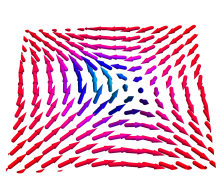
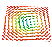
Figure 1: The isovector fields $\vec{\phi}$ of the $(1/2)_{N}$ (left plot) and $\left(1/2\right)_{S}$ (right plot) gauged merons in the $x-y$ plane for $g=0.5$, $m=1$.

We can now construct gauged merons numerically. For the sake of simplicity we set $c=0$, it yields two types of solutions $n\left(1/2\right)_{N,S}$. In our numerical simulations we start from an initial field configuration for an $(1/2)_{S}$-meron, which is produced by the rotationally invariant ansatz in polar coordinates in the $x-y$ plane:

$$\vec{\phi}=(\sin f\cos n\theta,\sin f\sin n\theta,\cos f)\,,A_{r}=0\,,A_{\theta}=A(r)\,,$$ (5)

where $f(r)\in\left[\pi,\pi/2\right)$. An input for a multimeron configuration can be constructed via product ansatz in stereographic notation, for example two-meron configuration corresponds to

$$W^{(1+2)}=W^{(1)}W^{(2)}\sqrt{\frac{1+c}{1-c}},\ A_{i}^{(1+2)}=A_{i}^{(1)}+A_{i}^{(2)}$$ (6)

where $W=\frac{\phi_{\perp}}{1+\phi_{3}}$. However, in our calculations we do not adopt any a priori assumptions about spatial symmetries of components of the field configuration.

As is well known, the asymptotic behavior of the scalar and magnetic fields almost completely determines the character of interaction between the solitons Gladikowski:1995sc ; Jaykka:2010bq ; Speight:1996px . Note that the rotational invariance of an isolated meron together with the gauge invariance with respect to the transformations (2) and asymptotic boundary conditions (3) implies that a spacial rotation of the configuration can always be compensated by an appropriate gauge transformation. In other words, the asymptotic form of the planar components of the scalar field $\phi_{\perp}$ and relative orientation of the solitons does not play a special role in the pattern of interaction between the gauged merons.

Linearization of the field equations of the model (1) yields the asymptotic decay of the fields of the meron

$$\phi_{3}(r)\sim c_{s}K_{0}(mr),\ A_{\theta}(r)\sim n+c_{v}rK_{1}(gr)\,,$$ (7)

where $K_{i}$ are $i$-th modified Bessel functions of the second kind and $c_{s},c_{v}$ are two constants which can be evaluated numerically. In particular, we found that for $(1/2)_{S}$ configuration (5) at $m=1$ and $g\in[0,1.5]$ these parameters are $c_{v}\simeq-1$ and $c_{s}\in[-3.5,-1.6]$. Below, we will make use of these values to evaluate the net force of the interaction between the gauged merons, see Fig. (2).

Note that both fields are massive and have form of scalar monopole and vector dipole. In the decoupling limit $g\to 0$, one of the components of the scalar field remains massless, $\sim d/r$, in the far field limit it corresponds to a source with dipole strength $d$ Jaykka:2010bq .

Using asymptotic (7) and considering the two meron configuration (6), we can evaluate the potential energy of the short-range Yukawa interaction between two static separated merons $U_{int}=E^{(1+2)}-E^{(1)}-E^{(2)}$

$$U_{int}=2\pi\left(c_{v}^{(1)}c_{v}^{(2)}K_{0}(gr)-c_{s}^{(1)}c_{s}^{(2)}K_{0}(mr)\right)$$ (8)

This formula exactly corresponds to the asymptotic intervortex potential in the Abelian Higgs model Speight:1996px , however the character of interaction depends on the type of the solitons. The force between the merons can be evaluated as

$$F=-U^{\prime}_{int}=\pm 2\pi c_{s}^{2}m(\eta^{2}g/mK_{1}\left(gR)-K_{1}(mR)\right)$$ (9)

where $\eta=c_{v}/c_{s}$ and the sign $"+"$ corresponds to the interaction between the merons of the same type in the $NN$-pair (or in the $SS$-pair). The opposite sign corresponds to the interaction between the merons of different types, they form the $NS$-pair.

Next, for each particular value of the gauge coupling $g$ we can evaluate the separation $R_{0}:\ F(R_{0})=0$, at which the forces between the merons are balanced. We expect that there will be a stable equilibrium for the system of two merons of different types, $N$ and $S$, whereas the interforce balance between the pairs of $S$ or $N$ merons will be unstable. Indeed, by analogy with the case of the interaction between the vortices in the Abelian Higgs model Speight:1996px , $NN$ (or $SS$) merons repel each other for $g/m<1$, and merge in the opposite case, forming rotationally invariant configuration with multiple magnetic flux. However, unlike the vortices, the merons may still repel at the small reparations, see Fig. (2), right plot.

The results of numerical simulations are summarized in Fig. 2, there, without loss of generality, we fix $m=1$. We confirm that the approximation of the intersoliton force (9) works very well, it correctly predicts the separation between the $N$ and $S$ merons in a stable equilibrium, see Fig. (2), left plot. Remarkably, the pair does not form a rotationally invariant configuration for any values of the gauge coupling, there is a short-range repulsive force between the merons of different type and the $NS$-pair remains separated.

The equilibrium between the merons of the same type is unstable, furthermore, in the case of the weak gauge coupling the separation between the merons becomes rather small and the asymptotic evaluation above breaks down, see Fig. (2), right plot.

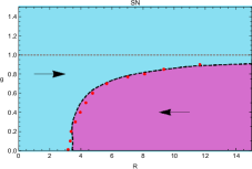
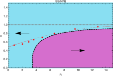
Figure 2: Interaction of the gauged merons in the $SN$-pair (left) and in the $NN(SS)$-pair (right). Arrows show the direction of the force. The blueish area corresponds to the scalar field domination region, the purple area represents the vector field domination region. Black dashed line indicates the equilibrium curve $F=0$, the red dots indicate the numerical solutions of full 2d minimization of the static energy of the system (1).

Multimeron configurations.  We observe that as $g\gtrsim 1$ the $NN(SS)$-pair always tends to merge into a rotationally invariant configuration with double magnetic flux for any initial separation between the merons. More generally, in the strong coupling regime the system of $n$ separated gauged merons of the same type evolves towards rotationally invariant configuration with $n$ units of magnetic flux. In Fig. 3, we present the results of the full numerical minimization of the energy functional for the $n\left(1/2\right)_{S}$ configurations with $n=1-4$. As expected, the field components become less localized and the core of the vortex is expanding, as the winding number $n$ increases. The energy density distribution of the $n=1$ configuration reaches its maximum value at the center of the soliton, for $n>1$ it has a shape of a circular wall with a local minimum at the origin. Field components of these solutions along $x$ axis are displayed in Fig. 3 (top row), both $\phi_{1}$ and $\phi_{3}$ decay exponentially, however at $g=4$ the former component approaches the vacuum faster than the latter.

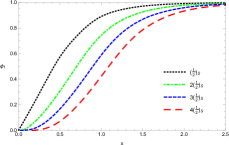
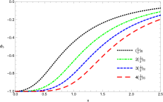
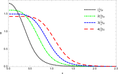
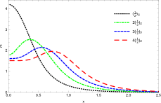
Figure 3: Rotationally invariant $n\left(1/2\right)_{S}$ configurations: Profiles of the field components $\phi_{1}$ (upper left) and $\phi_{3}$ (upper right), the distributions of the magnetic field (bottom left) and the energy density (bottom right) along the $x$-axis for $n=1-4$, $g=4$ and $m=1$.

Evaluation of the intersoliton forces above indicates that for $m=1$ and $0.57\lesssim g<1$ we could construct stable multisoliton configuration with merons of both types. Indeed, it is seen in Fig. 4, which displays contour plots of the magnetic field and the energy density distribution of various solutions which we constructed numerically, in such a case the rotational symmetry becomes broken and the gauged merons form configurations with discrete symmetry.

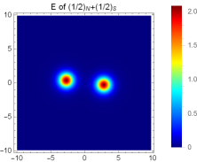
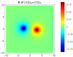
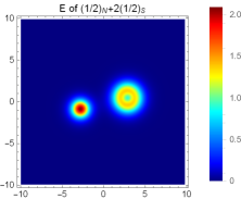
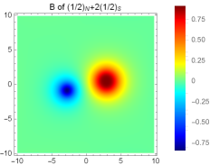
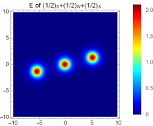
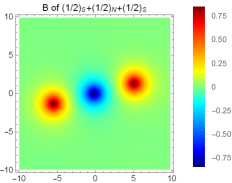
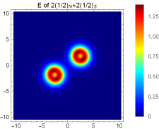
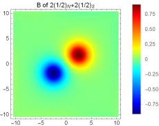
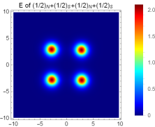
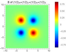
Figure 4: Contour plots of the energy density (left column) and magnetic field (right column) of given meron configurations at $g=0.7$, $m=1$.

Note, that the $(1/2)_{S}+(1/2)_{N}$ pair combines a short-range repulsion and a long-range attraction, forming a weakly bound system. Certainly, there is a similarity with the aloof baby Skyrmions constructed in Salmi:2014hsa . Further, the binary particle model suggested in Salmi:2014hsa also can be implemented in the case of the gauged multimeron configurations.

Our numerical results presented in Fig. 4 agree well with the qualitative discussion of the intersoliton interaction above, see Fig. 2, as the separation between the merons of the same type is relatively small, they tend to merge into a symmetric configuration which carriers multiple magnetic flux. On the other hand, widely separated merons repel each other. The energy per meron is decreasing as the number of components is increasing, thus the system is stable with respect to decay into constituents. Also the configurations with constituents possessing multiple units of magnetic flux, like for example $(1/2)_{N}+2(1/2)_{S}$, have lower energy than the chain $(1/2)_{N}+(1/2)_{S}+(1/2)_{N}$. The latter configuration represents a local minimum of the energy functional.

Finally, we would like to comment on the limit of the single vacuum potential, setting $c=\pm 1$ reduces it to $V(\vec{\phi})=m^{2}(1\mp\phi_{3})^{2}$. In this limit the magnetic flux is no longer topologically quantized. However, numerical simulations show that in the strong gauge coupling limit, it becomes quantized again Gladikowski:1995sc ; Samoilenka:2015bsf . We can understand the underlying topological reason for this when we note that the maxima of the magnetic field corresponds to the points, where $\phi_{3}=\pm 1$, see Fig. 4. In the limit $g\to\infty$ the magnetic field is completely localized at the origin, then the potential of the gauge field becomes a pure gauge everywhere apart this point and the magnetic flux is entirely determined by the Poincaré index of the planar components $\phi_{\perp}$. Similar pattern also holds for the gauged Hopfion solutions in the Faddeev-Skyrme model Shnir:2014mfa .

Conclusions.   Our investigation confirms the existence of new type of regular finite energy solutions of the planar Maxwell-Skyrme model, the gauged merons. They carry topologically quantized magnetic flux and possess fractional topological charges in the scalar sector. The vortex winding number is set into correspondence with the Poincaré index of the planar components of the meron. Considering the interaction between the gauged merons, we have shown that, unlike the usual vortices in the Abelian Higgs model, they may combine a short-range repulsion and a long-range attraction, forming a weakly bound non-rotationally invariant system. The resulting pattern of interaction is more complicated than that both for the usual vortices in the Abelian Higgs model, and for the solitons in the gauged baby Skyrme model. It remains a major challenge, deserving further study, to find a moduli space description for the low-energy dynamics of the gauged merons.

Acknowledgments.   Y.S. thanks Nick Manton, Muneto Nitta and Nobuyuki Sawado for helpful discussions. He gratefully acknowledges support from the Russian Foundation for Basic Research (Grant No. 16-52-12012), the Ministry of Education and Science of Russian Federation, project No 3.1386.2017, and DFG (Grant LE 838/12-2). The numerical computations were performed on the HybriLIT cluster, JINR, Dubna.

References

- (1) Solitons and Condensed Matter Physics, edited by A. R. Bishop and T. Schneider (Springer-Verlag, Berlin, 1978).
- (2) P.J. Ackerman and I.I. Smalyukh, Phys. Rev. X , 7, 011006 (2017)
- (3) A.M. Kosevich, The crystal lattice: phonons, solitons, dislocations, superlattices, (John Wiley Sons, 2006).
- (4) L.F. Mollenauer and J.P. Gordon, Solitons in Optical Fibers, (Academic Press, 2006).
-
(5)
T. Dauxois and M. Peyrard, Physics of Solitons, (Cambridge University Press, 2006)
M. Peyrard, Nonlinear Excitations in Biomolecules, (Springer-Verlag, , 1995). - (6) N. Manton and P. Sutcliffe, Topological Solitons, (Cambridge University Press, 2004).
- (7) A. Vilenkin and E.P.S. Shellard, Cosmic Strings and Other Topological Defects, (Cambridge University Press, Cambridge, England, 1994).
- (8) T.H.R. Skyrme, Proc. Roy. Soc. Lond. A 260, 127 (1961)
- (9) A.A. Bogolubskaya and I. L. Bogolubsky, Phys. Lett. A 136, 485 (1989)
- (10) X.Z. Yu et al, Nature, 465, 901 (2010)
- (11) S. Mühlbauer et al, Science, 323, 915 (2009)
-
(12)
A.N. Bogdanov and D. A. Yablonsky,
Sov. Phys. JETP 95, 178 (1989);
A.N. Bogdanov, JETP Lett. 62, 247 (1995) - (13) S. Heinze, et al, Nature Phys. 7, 713 (2011)
- (14) J.P. Liu, Z. Zhang, and G. Zhao, eds., Skyrmions: Topological Structures, Properties, and Applications, (CRC Press, 2016).
- (15) A. Neubauer et al, Phys. Rev. Lett. 102, 186602 (2009)
- (16) J. Gladikowski, B. M. A. G. Piette and B. J. Schroers, Phys. Rev. D 53, 844 (1996).
- (17) B.J. Schroers, Phys. Lett. B 356, 291 (1995).
- (18) C. Adam, C. Naya, J. Sanchez-Guillen and A. Were-szczynski, Phys. Rev. D 86, 045010 (2012).
- (19) A. Samoilenka and Y. Shnir, Phys. Rev. D 93, 065018 (2016).
- (20) C. Adam and A. Wereszczynski, Phys. Rev. D 95, 116006 (2017).
- (21) F. Navarro-Lerida, E. Radu and D. H. Tchrakian, Phys. Rev. D 95, 085016 (2017).
- (22) A. Samoilenka and Y. Shnir, Phys. Rev. D 95, 045002 (2017).
- (23) P. Eslami, M. Sarbishaei and W. Zakrzewski, Nonlinearity, 13, 186 (2000).
- (24) J. Jaykka and M. Speight, Phys. Rev. D 82, 125030 (2010).
- (25) M. Kobayashi and M. Nitta, Phys. Rev. D 87, no. 12, 125013 (2013).
- (26) D. J. Gross, Nucl. Phys. B 132, 439 (1978).
- (27) M. Nitta and W. Vinci, J. Phys. A 45, 175401 (2012).
- (28) S. Z. Lin, A. Saxena and C. D. Batista, Phys. Rev. B 91, 224407 (2015).
- (29) Y. Brihaye, B. Hartmann and D. H. Tchrakian, J. Math. Phys. 42, 3270 (2001).
- (30) J. Jaykka and M. Speight, Phys. Rev. D 82, 125030 (2010).
- (31) J. M. Speight, Phys. Rev. D 55, 3830 (1997).
- (32) P. Salmi and P. Sutcliffe, J. Phys. A 48, 035401 (2015).
- (33) Y. Shnir and G. Zhilin, Phys. Rev. D 89, 105010 (2014).