Metal-Rich RRc stars in the Carnegie RR Lyrae Survey

Abstract

We describe and employ a stacking procedure to investigate abundances derived from the low S/N spectra obtained in the Carnegie RR Lyrae Survey (CARRS; Kollmeier et al. 2013). We find iron metallicities that extend from [Fe/H] $\sim$  $-$2.5 to values at least as large as [Fe/H] $\sim$ $-$0.5 in the 274-spectrum CARRS RRc data set. We consider RRc sample contamination by high amplitude solar metallicity $\delta$ Scuti stars (HADS) at periods less than 0.3 days, where photometric discrimination between RRc and $\delta$ Scuti stars has proven to be problematic. We offer a spectroscopic discriminant, the well-marked overabundance of heavy elements, principally [Ba/H], that is a common, if not universal, characteristic of HADS of all periods and axial rotations. No bona fide RRc stars known to us have verified heavy-element overabundances. Three out of 34 stars in our sample with [Fe/H] $>$ $-$0.7 exhibit anomalously strong features of Sr, Y, Zr, Ba, and many rare earths. However, carbon is not enhanced in these three stars, and we conclude that their elevated $n$-capture abundances have not been generated in interior neutron-capture nucleosynthesis. Contamination by HADS appears to be unimportant, and metal-rich RRc stars occur in approximately the same proportion in the Galactic field as do metal-rich RRab stars. An apparent dearth of metal-rich RRc is probably a statistical fluke. Finally we show that RRc stars have a similar inverse period-metallicity relationship as has been found for RRab stars.

1 INTRODUCTION

The apparent paucity of metal-rich ([Fe/H] $>$ $-$1.0) RRc stars in the Galactic field has received passing mention during the past few decades, viz., Smith (1995). Only DH Peg, one of the several possible metal-rich RRc candidates in an early spectroscopic survey (Preston, 1959) survived subsequent photometric reclassification, and its membership is debated (Fernley et al., 1990). We are aware of no other bona fide metal-rich RRc star in extant literature. None of the twenty RRc in the Hipparcos catalog, chosen primarily by proximity to the Sun, are metal-rich (Feast et al., 2008), nor are any of the nineteen RRc chosen for abundance analysis solely by location in the sky at Las Campanas Observatory (Sneden et al., 2017). However, such stars ought to exist: theoreticians happily compute families of low mass, metal-rich, core helium-burning first overtone pulsators, i.e., metal-rich RRc stars (Marconi et al., 2015). This is a puzzle that as yet does not have a satisfactory resolution.

The data set of Kollmeier et al. (2013) (hereafter in this paper K13) provides a provisional answer in the form of several dozen metal-rich RRc candidates. These stars form the observational basis of the present investigation in which we confront two issues. (1) Low signal-to-noise ($S/N$) of individual stellar echelle spectra, the price paid for the rich harvest of the metal-rich candidates, renders conventional abundance analysis problematical. (2) Possible contamination of the K13 metal-rich RRc sample by high amplitude $\delta$ Scuti stars (HADS) and/or other related members of the near-main-sequence zoo of pulsating stars (Rodríguez et al. 2000; see discussion of their Table 12), all of which possess more or less solar abundances. DH Peg illustrates the problem. Antonello et al. (1986, §5) report, with particular reference to DH Peg, that Fourier decomposition of light curves provides no clear distinction between HADS and RRc stars. Following Antonello et al., Fernley et al. (1990, §4.1) conclude their analysis of DH Peg with the remark that “DH Peg is most likely an RR Lyrae, but the classification has to be treated with some caution”.

We address possible contamination of the K13 sample by $\delta$ Sct stars that abound in the solar neighborhood: 636 are listed in the catalogue of Rodríguez et al. (2000). Of these, 54 have $P$ $>$ 0.20 d and of these 26 (4%) are HADS, having light amplitudes $\Delta V$ $>$ 0.3 mag, values permitted for inclusion in the K13 survey. Therefore we need (and have found) an effective RRc/$\delta$Sct discriminant as we will describe below.

We reconsider the K13 274-spectrum RRc sample in §2 and §3, demonstrating that their low $S/N$ spectra yield reliable overall [Fe/H] metallicities. In §4 we show that three program stars have significant overabundances of neutron-capture ($n$-capture, atomic number $Z$ $>$ 30) elements, and identify these as probable $\delta$ Sct variables. Finally, in §5 we validate the existence of an anticorrelation between [Fe/H] and pulsational period $P$ in RRc stars analogous to the well-known anti-correlation for RRab stars.

2 THE SPECTROSCOPIC DATASET

The K13 sample began with the RRc variables identified in the All Sky Automated Survey catalog (ASAS; Pojmanski 2002, Pojmanski et al. 2005 and references therein). Szczygieł & Fabrycky (2007) and Szczygieł et al. (2009) examined the ASAS RRc light curves for evidence of the Blazhko effect (a slow variation in photometric and spectroscopic periods and amplitudes of some RR Lyrae stars). The K13 star list did not include any Blazhko variables found in those papers. Proper motions were taken from USNO CCD Astrograph Catalogs (Zacharias et al., 2004, 2013). High-resolution spectroscopy of candidate RRab and RRc stars was undertaken to provide accurate radial velocities and approximate values of metallicities. K13 considered only RRc stars, with the RRab sample to be considered later.

The spectra for the K13 snapshot RR Lyrae survey were gathered in 2011-12 with the echelle spectrograph of the Las Campanas Observatory 2.5m du Pont Telescope. The spectrograph configuration was identical to that employed in a series of papers on the velocities, H$\alpha$ profiles, metallicities, and relative abundance ratios of RR Lyrae stars (For et al. 2011a, b, Govea et al. 2014, Chadid et al. 2017, Sneden et al. 2017). The spectrograph with a 1.5$\times$4.0 arcsec aperture delivered resolving power $R$ = $\lambda/\Delta\lambda$ $\sim$ 27000 at 5000 Å. The spectral coverage was $\lambda\lambda$ 3400–9000, with wavelength gaps in the CCD order coverage beginning at $\lambda$ 7100 Å and growing with increasing wavelength. In practice the useful spectral domain for this work was limited to $\lambda\lambda$ 3900–7000 Å.

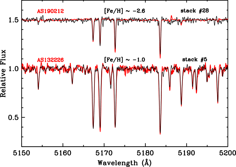
Figure 3: Comparison of our stacked spectra (black lines) and ond those selected from the Sneden et al. (2017) RRc study (red lines) in spectral region surrounding the Mg i b lines. The two examples are among the most metal-poor and metal-rich of the RRc study.

The K13 spectra were taken as close as possible to a target pulsational phase $\phi$ = 0.32, which is the phase of the time-averaged velocity on the ascending branch of the RV curve (with respect to visual maximum light defined as $\phi$ = 0) for the RRc variables T Sex and TV Boo (Liu & Janes, 1989), DH Peg (Jones et al., 1988), and YZ Cap (Govea et al., 2014).. The phase and radial velocity issues are discussed in §3 of K13. The target phase was achieved in their 261-star RRc sample, as illustrated in K13 Figure 3; we calculate $\langle\phi\rangle$ = 0.333 ($\sigma$ = 0.024). The reduction path from observed CCD frames to final wavelength-calibrated multi-order spectra used a software pipeline designed and implemented by Kelson (2003). Continuum-normalized and order-concatenated spectra were produceed with the IRAF ECHELLE package. The observed RRc sample is given in Table 1, identified by their ASAS number. This table is ordered according to derived K13 metallicity, with the highest first (124115–4056.9, [Fe/H] = $+$0.04) and the lowest last (195307-5131.1, [Fe/H] = $-$2.78) Among the listed quantities taken from the ASAS database are $V_{max}$, the mean visual magnitude at maximum light and $V_{amp}$, the visual light amplitude (the defined zero point of pulsational phase $\phi$). There were 274 observed spectra, and with 13 stars observed twice, the total number of stars was 261. In the present paper we treat individual spectra as independent objects.

The K13 metallicity estimates were made by matching the observed spectra to a grid of synthetic spectra, as described in their §3.3. RRc stars have well-determined photometric properties with relatively small variations throughout their pulsational cycles. Mean absolute magnitudes are $\langle M_{V}\rangle$ = $+$0.6 $\pm$ 0.1 (K13) and cyclical variations are $\langle M_{amp}\rangle$ $\simeq$ 0.25 (Table 1). Similarly, $\langle(B-V)_{amp}\rangle$ $\sim$ 0.2 (e.g., Figure 3 of Layden et al. 2013). The small variations in these photometric quantities combined with the very small observed pulsational phase range centered at $\phi$ = 0.33 allowed K13 to adopt a single set of atmospheric parameters except overall metallicity, based on their analysis of higher $S/N$ du Pont echelle spectra of the RRc star YZ Cap (not included in the K13 sample). The values derived for YZ Cap were effective temperature T_eff = 7000 K, surface gravity log g = 2.2, microturbulent velocity $\xi_{\rm t}$ = 2.5 km s^-1, and $\alpha$ element enhancement [$\alpha$/Fe] = +0.35.

The wavelength regions studied by K13 were limited to a “blue” spectral interval 4400$-$4675 Å and a “yellow” interval 5150$-$5450 Å. The chosen yellow interval contains many neutral-species metal transitions, and especially includes the Mg i b lines; this triplet remains easily detectable even in the most metal-poor RRc target. The majority of strong lines in the blue interval are due to metal ions, such as Ti ii and Fe ii. This region also contains the Ba ii 4554 Å line that is often used to identify potential neutron-capture-rich stars, and proved to be of importance to the present investigation. Other spectral regions were ignored, for various reasons. Briefly, the observed spectra extend significantly blueward of 4400 Å and they display many useful spectral absorption features. Unfortunately, the $S/N$ of these snapshot spectra declines substantially below 4400 Å, rendering this spectral region less useful for metallicity estimates. The yellow-red regions beyond 5450 Å have adequate $S/N$, but our warm, metal-poor RRc stars have very few strong lines in this wavelength domain; many intervals appear to be close to pure continua. The region between 4675 and 5150 Å has a few potentially useful lines, but it includes H$\beta$ at 4861 Å, whose broad wings complicate abundance analysis.

In K13 the line lists for synthetic spectra began with the Kurucz (2011) database followed by syntheses of the solar spectrum in order to adjust the line parameters (mostly their transition probabilities). Model atmospheres were interpolated among the Kurucz ATLAS model grid, and synthetic spectra were computed with the current version of the MOOG synthetic spectrum code (Sneden, 1973). The model grid was computed from $+$0.05 $\geq$ [Fe/H] $\geq$ $-$2.90. K13 then used reduced $\chi^{2}$ minimization (weighting by $S/N$) to estimate [Fe/H] values separately in the blue and yellow spectral regions. Within each region estimates were made covering the whole interval and one more narrowly confined to a set of the strongest lines. Thus four metallicity estimates were made for each RRc star.

In Table 1 for each star we list the mean $S/N$ of the values in the blue and yellow spectral intervals, and the mean K13 [Fe/H] derived from the four individual estimates. A simple average yields $\langle S/N\rangle$ = 18.5 ($\sigma$ = 6.6). The average scatter of the four [Fe/H] estimates leading to the final values in Table 1 is $\langle\sigma\rangle$ = 0.18; this is a reasonable estimate of internal uncertainties in the K13 metallicity values.

3 NEW RRC METALLICITIES FROM CO-ADDED SPECTRA

The low $S/N$ of the K13 spectra precludes the kind of line-by-line model parameter and abundance analysis done in our previous RR Lyrae studies cited above. Given the narrow range of RRc stellar atmosphere quantities and the large number of stars in all metallicity domains, we decided to co-add the K13 spectra in small metallicity bins in order to significantly increase their $S/N$ so that a more traditional investigation could be undertaken.

3.1 Stacking the Spectra

Beginning at the high-metallicity end of the K13 program stars, we averaged successive sets of 10 spectra, weighting the means by the $S/N$ of each spectrum. We will refer to these mean spectra as “stacks” and their properties (metallicity, temperature, etc.) as “stack” properties. With 274 program stars, there were 28 stacks, with the lowest metallicity stack#28 continuing just four spectra. Additionally, for reasons to be developed below, we believe that three stars in stack#1 are not members of the RRc class. These stars are labeled “no” in the last column of Table 1. Since these three do not appear to be true RRc stars, this stack contains only seven spectra. We list the 28 stacks in Table 2. For each stack we give the number of stars, the mean K13 [Fe/H] values, the spread of the K13 metallicity values $\Delta$[Fe/H], model atmosphere parameters (see §3.2), and the mean pulsational periods. As illustrated in the K13 Figure 1 metallicity histogram, there are comparatively few stars at the high and low metallicity ends of our sample, and a large pile-up near [Fe/H] $\simeq$ $-$1.2; this is reflected in the different $\Delta$[Fe/H] values in Table 1.

In Figure 1 we show a typical example of the improvement in $S/N$ achieved by the stacking procedure. A small part of the K13 blue spectral region has been chosen to illustrate a difficult $S/N$ regime. The stack#15 co-added spectrum ([Fe/H]_K13 = $-$1.26) is shown along with two of its constituent spectra that were chosen to represent the highest and one of the lowest $S/N$ values. For stack#15 in the blue we estimate $S/N$ $\sim$ 40 as indicated in the figure, and in the yellow $\sim$ 60; values for other stacks are comparable.

3.2 Stack Analyses

We treated each stack as an observed stellar spectrum, and derived atmospheric quantities in the same manner as done by Chadid et al. (2017), Sneden et al. (2017), and references therein. The line analysis code and model atmosphere databases were as described in §2. However, unlike the K13 linelists developed by matching the solar spectrum in two regions, for this work we expanded the spectral range to 3900$-$6500 Å and used only unblended absorption lines with laboratory transition probabilities. Because the present study concentrates on Fe metallicities and just a few indicators of elemental group relative abundances, we list only the most important $gf$-value sources (see Sneden et al. 2016 for extended comments). $(a)$ Fe i: O’Brian et al. (1991) for lines with excitation energies $\chi$ $<$ 2.4 eV and Den Hartog et al. (2014), Ruffoni et al. (2014) for higher excitation lines. $(b)$ Fe ii: the NIST Atomic Spectra Database (Kramida et al., 2015). $(c)$ Ti ii: Wood et al. (2013); a few Ti i lines were also measured, and the $gf$’s of Lawler et al. (2013) were used, but they provided only a weak check on the Ti abundances derived from ionized lines.

Standard excitation equilibrium constraints and weak-line/strong-line balance on Fe i transitions were used to iteratively derive T_eff and $\xi_{\rm t}$, respectively. Ionization balance between Fe i and Fe ii yielded log g, and derived [Fe/H] values were checked for consistency with input model metallicities. We list these quantities for the stacks in columns 5$-$8 of Table 2. The variations in these quantities over the complete set of stacks (e.g., over the whole RRc metallicity range) are modest: $\langle\mbox{T${}_{\rm eff}$}\rangle$ = 7015, $\sigma$ = 90 K; $\langle\mbox{log~{}{\it g}}\rangle$ = 2.6, $\sigma$ = 0.3; and $\langle\mbox{$\xi_{\rm t}$}\rangle$ = 2.7, $\sigma$ = 0.5.

More importantly, the newly-derived stack [Fe/H] values correlate well with the mean K13 stack metallicities. Taking differences in the sense $\Delta$[Fe/H] $\equiv$ [Fe/H]_K13 $-$ [Fe/H]_new, the average is $\langle\Delta$[Fe/H]$\rangle$ = $-$0.11 $\pm$ 0.03 ($\sigma$ = 0.17). However, there is a small, nearly linear drift with metallicity in the $\Delta$[Fe/H] values, as we illustrate in Figure 2. A linear regression line is [Fe/H]_new,pred = 0.75[Fe/H]_K13 $-$ 0.44 with correlation coefficient $r$ = 0.98. The scatter of points around this trend line is very small, $\sigma$ = 0.08.

Overall we regard comparison between our new stack metallicities and those of K13 as very good. There are a number of possible causes for the slope of the regression seen in Figure 2; here we list a few of the more likely explanations. First, continuum normalizations are difficult to do self-consistently at the low $S/N$ of the original K13 spectra. This is caused by the more than two dex metallicity range of the stellar sample, which created large differences in line density in both the original blue and yellow spectral regions. Second, the K13 $\chi^{2}$ metallicity estimation technique was fairly simple. In that study it was easiest to find reliable $\chi^{2}$ minima in the higher metallicity regime. Third, the new analysis relies on laboratory transition data for individual spectral lines; K13 based their spectrum syntheses on line lists that matched the solar spectrum. However, the basic result here is that the K13 metallicities correlate well with standard abundance analyses; the grid synthesis method yielded reliable metallicities even when the spectral $S/N$ values were very low.

In Figure 3 we compare two stacked spectra with those of two individual RRc stars from Sneden et al. (2017, hereafter S17), displaying a portion of the wavelength region that has the prominent Mg i b line triplet. That study observed 19 RRc stars throughout their pulsational cycles, combining new data with those published by Govea et al. (2014). Typically about 40 spectra per star were gathered, enough so that multiple observations at one phase interval ($\delta\phi$ $\simeq$ $\pm$0.05) could be combined to achieve fairly high $S/N$. Here we consider two stars at the extremes of the Sneden et al. metallicity range. The S17 RRc stars were analyzed both from spectra at individual phases and from co-additions into stellar spectrum means. Star 190212-4639.2 (also part of the K13 survey) was analyzed in various ways, leading to [Fe/H] = $-$2.65, with probable uncertainty $\simeq\pm$0.15. That star is a member of stack#28, which has [Fe/H]_K13 = $-$2.69 and [Fe/H]_new = $-$2.42 (Table 2). For Figure 3 we have displayed the pulsational phase $\phi$ = 0.331 S17 spectrrum, for which they derive [Fe/H] = $-$2.62 with $\sigma$ = 0.16. This spectrum is virtually indistinguishable from that of stack#28 in the figure. At the high metallicity end, we display the S17 spectrum of 132226-2042.3 (with [Fe/H] = $-$0.95, probable uncertainty $\simeq\pm$0.15) and that of our stack#5 ([Fe/H]_K13 = $-$0.80, [Fe/H] = $-$1.03). We have chosen to show their $\phi$ = 0.448 spectrum, for which they derive [Fe/H] = $-$1.03. Again, visual comparison of the spectra in Figure 3 suggests excellent agreement.

We have not made extensive chemical composition analyses of the stacked spectra for which the $S/N$ values remain modest after stacking. However, usually there are enough Ca i and Ti ii lines to check relative abundances in the $\alpha$ element group. For the 28 stacks we derive $\langle$[Ca/Fe]$\rangle$ = $+$0.25 ($\sigma$ = 0.13) and $\langle$[Ti/Fe]$\rangle$ = $+$0.50 ($\sigma$ = 0.20). These reproduce, with large scatter especially for Ti, the well-known $\alpha$-element overabundances in metal-poor stars. We also note that for stack#1, our highest metallicity spectrum, we derive [Ca/Fe] $\simeq$  [Ti/Fe] $\simeq$ 0.0, as expected for relatively metal-rich stars. More detailed abundance analyses are not justified here.

4 $\delta$ SCUTI STARS HIDING IN PLAIN SIGHT

As outlined in §1 metal-rich RRc stars are difficult to distinguish from high amplitude $\delta$ Scuti stars (HADS) by multi-color photometry. Fortunately a clear spectroscopic signal exists: (relatively) slowly rotating $\delta$ Scuti stars have enhanced abundances of heavy elements, generally rising with increasing atomic number to become extremely high in the $n$-capture domain ($Z$ $>$ 30). We illustrate this by gathering literature [Fe/H] and [Ba/H] values for HADS and plotting them in Figure 4. Panel (a) of this figure shows that the Fe abundances have some star-to-star scatter, but with a nearly solar mean: $\langle$[Fe/H]$\rangle$ = $+$0.12 ($\sigma$ =0.20, 23 stars). Several stars with $vsini$ $<$ 100 km s^-1 have [Fe/H] $>$ $+$0.2, which may be a sign of the general elevation of heavy element overabundances of $\delta$ Scuti stars. However, relative abundances of Ba ($Z$ = 56) displayed in panel (b) are all supersolar, all having [Ba/Fe] $\gtrsim$ $+$0.2. The majority of these $\delta$ Scuti’s have [Ba/H] $\gtrsim$ 0.5, and six have have [Ba/H] $\gtrsim$ 1.

We searched the higher metallicity K13 spectra for signs of $n$-capture overabundances. In spite of the low $S/N$ of these spectra, three stars were easily spotted with unusually strong Ba ii 5853 Å lines: ASAS 095845-5927.8, 195123+0835.0, and 141107-4212.2 (tagged with “no” entries in Table 1). This is significant because normally this line cannot be easily detected in the K13 spectra even in the metal-rich domain. Therefore, we formed a mean spectrum of these three Ba-strong stars and subjected it to the same analysis as described above for the stack spectra. We derived model parameters T_eff = 6900 K, log g = 3.0, $\xi_{\rm t}$ = 3.2 km s^-1, and [Fe/H] = $-$0.45. These values are similar to those of stack#1 except for the gravity: log g is greater by 0.4 dex in the Ba-strong mean spectrum.

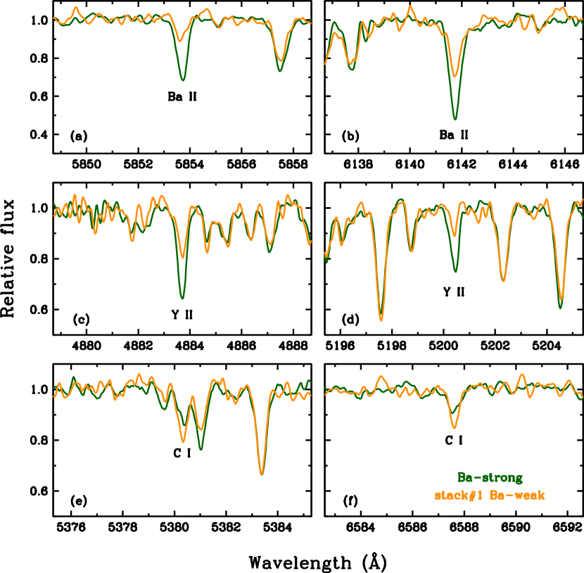
Figure 5: Six small spectral windows chosen to display features of Ba, Y, and C in stack#1 (orange lines) and Ba-strong (green lines) spectrum. As described in the text, the Ba-strong spectrum is the mean of the spectra that were excluded from stack#1 due to their high $n$-capture line strengths.

The heavy element overabundances of Ba-strong stars are obvious by inspection of relevant transitions. Figure 5 presents the spectroscopic evidence. Panels (a) and (b) show the Ba ii 5853 Å and 6141 Å lines of stack#1 and those of a co-addition of the three Ba-strong stars excluded from this stack. Significant Ba strength differences are evident, most clearly for the 5853 Å line. The 6141 Å feature is partially blended with an Fe i line, lessening the total difference. These sharp contrasts in Ba ii strengths are shared by very strong 4554 Å, strong-but-blended 4934 Å, clean and strong 6496 Å, and high excitation weak-but-blended 4130 Å. We computed synthetic spectra of the 4554, 5853, 6141, and 6496 Å lines, deriving $\langle$[Ba/H]$\rangle$ = $-$0.58 ($\sigma$ = 0.16) for stack#1 and $\langle$[Ba/H]$\rangle$ = $+$1.00 ($\sigma$ = 0.15) for the Ba-strong spectrum. The 1.6 dex overabundance in the Ba-strong stars confirms the Ba ii line strength differences seen in Figure 5. However, much caution is warranted on the magnitude of the overabundance, because nearly all Ba ii lines are very saturated in the Ba-strong stars. Therefore they are sensitive to adopted $\xi_{\rm t}$ and to outer-atmosphere line formation effects that are not accounted for in our standard modeling approach. Such very strong lines typically yield unrealistically large abundances of Fe-group elements in RRc stars, and thus are ignored in our model analyses.

Fortunately other heavy $n$-capture elements are easily detected in our Ba-strong stars: La ($Z$ = 57), Eu (63), and to a lesser extent Nd (60). Six lines of La ii are seen, and the most useful ones at 4123, 4920, and 4921 Å yield for the mean three-star Ba-strong spectrum $\langle$[La/H]$\rangle$ $\simeq$ $+$0.2, while for the stack#1 spectrum we obtain $\langle$[La/H]$\rangle$ $\simeq$ $-$0.4. Lines of Eu ii at 4129 and 4205 Å suggest $\langle$[Eu/H]$\rangle$ $\simeq$ $+$0.4 for the Ba-strong stars while they are undetectable in the stack#1 spectrum. Taken together, the three heavy $n$-capture elements have [X/H] $\sim$ $+$0.2 to 1.0, or [X/Fe] $+$0.7 to $+$1.5 in the Ba-strong spectrum while the stack#1 spectrum has [X/H] = $-$0.6 to $-$0.4 or [X/Fe] =  $-$0.1 to $+$0.1.

The overabundances extend to the lighter $n$-capture elements Sr, Y, and Zr ($Z$ = 38$-$40). Panels (c) and (d) of Figure 5 show that the Ba-strong stars exhibit much stronger Y ii lines than those of stack#1. From these lines we derive $\langle$[Y/H]$\rangle$ $\simeq$ $+$0.2, or $\langle$[Y/Fe]$\rangle$ $\simeq$ $+$0.6 in the Ba-strong stars, while two lines of Zr ii in the noisy and crowded 4200 Å spectral domain yield $\langle$[Zr/H]$\rangle$ $\simeq$ $+$0.4, or $\langle$[Y/H]$\rangle$ $\simeq$ $+$0.8. We did not attempt syntheses of the extremely strong Sr 4077 and 4215 Å resonance lines, but inspection of our spectra argues for the same abundance enhancement in Ba-strong stars for Sr as well.

In contrast, the evolutionary-sensitive light element C shows no abundance difference between the Ba-strong spectrum and that of stack#1. In fact, the C i high excitation lines ($\chi$ $>$ 7.5 eV) displayed in Figure 5 panels (e) and (f) appear to be weaker in the Ba-strong stars. This is confirmed by our spectrum syntheses of these two lines plus C i 5052 Å: $\langle$[C/H]$\rangle$ $\simeq$ $-$0.3 in the Ba-strong spectrum and $\langle$[C/H]$\rangle$ $\simeq$ $-$0.1 in stack#1. The lack of C enhancement in the Ba-strong spectrum is confirmed by our failed attempt to detect the CH G-band. Even at T_eff $\sim$ 7000 K, a substantial C overabundance would have produced measurable CH absorption near the bandheads in the 4300$-$4325 Å region.

In summary, all $n$-capture elements are very overabundant but C is not in the Ba-strong stars. Setting aside analytically-difficult Ba, we suggest that [$\langle$Y,Zr,La,Eu$\rangle$/Fe] $\simeq$ $\sim$ $+$0.7. This cannot be the result of rapid $n$-capture nucleosynthesis (the $r$-process), because the signature element of the $r$-process is greatly enhanced Eu/La values; this is contrary to our result. However, slow $n$-capture (the $s$-process) cannot be the cause either: not only is there no La/Eu overabundance, there is no evidence for enhanced C, which is a general characteristic of $s$-process-rich stars. We conclude that stellar evolutionary processes cannot be blamed for the large heavy element abundances in our Ba-strong stars. Therefore, we think that these stars are HADS.

5 CONCLUSIONS AND DISCUSSION

The two basic results of this paper are that (1) the K13 high resolution-but-low $S/N$ spectra of RRc candidates yield reliable [Fe/H] metallicities on average for RRc stars, and (2) among the K13 RRc sample there are a few high metallicity stars with overabundances of $n$-capture elements that identify them as $\delta$ Scuti stars. Here we consider the new metallicities in more detail. Following Chadid et al. (2017) and Sneden et al. (2017), we chose Layden’s (1995) division between metal-poor (MP) and metal-rich (MR) RRL stars at [Fe/H] = $-$1. The MR sample should be dominated by Galactic thin and thick-disk members, and the MP sample should contain mostly halo members. The exact choice of the MP/MR metallicity division is not important for our discussion.

The K13 RRc metallicities, now confirmed by our stacked-spectrum analyses, exhibit a small but statistically significant anti-correlation with photometric pulsational periods. An inverse relationship between [Fe/H] and period for RRab stars has been known for some time. Preston (1959) defined a metallicity-sensitive Ca ii K-line strength index $\Delta S$ from low-resolution spectra of about 100 RRab variables. His Figure 4 showed that the highest metallicity stars ([Fe/H] $\sim$ 0.0, $\Delta S$ $\sim$ 0) have periods $\langle P\rangle$ $\sim$ 0.4 days while the lowest metallicity stars ([Fe/H] $\sim$ $-$2.5, $\Delta S$ $\sim$ 10) have $\langle P\rangle$ $\sim$ 0.7 days. Preston also suggested that a period-metallicity anticorrelation exists for RRc stars, but this conclusion was based on only nine such stars in his sample.

In Figure 6 we use the data of Table 2 to show the metallicity-period relationship for our RRc spectrum stacks, plotting points for both the original K13 metallicities and those newly derived in this paper. The metallicity-period anticorrelation is evident in this plot. However, a few cautions should be borne in mind. First, note the “mean stack ranges” in the plot that is placed in the lower left corner. The dimensions of this cross were formed by calulating the means of the spreads of periods and metallicities in each of the 28 stacks. This is representative, but individual stacks can have larger/smaller spreads in either quantity. The ranges suggest that typical stacks have only small star-to-star scatter in [Fe/H] values but large scatter in their pulsational periods. Second, the points at the extreme metallicity ends should not be over-interpreted. For example, there are just four stars comprising the most metal-poor stack#28, and seven in the most metal-rich stack#1 (discussed in §4). Third, on our revised metallicity scale, the total number of MR stars is only 38 (14% of our sample).

With these caveats in mind, the metallicity-period trend for RRc stars is clear in Figure 6 whether the original K13 stack [Fe/H] values or the ones derived in this paper are used. The new metallicities and those of K13 agree at [Fe/H] $\sim$ $-$1.8, with the new scale yielding higher [Fe/H] values at the low metallicity end and lower at the high end (Table 2, Figure 2). The new metallicities thus steepen the slope of the RRc metallicity-period relationship. Additionally, the slope appears to be different in the MR and MP regimes (again, with either the K13 or the new metallicities). If one ignores our defined MR/MP split at [Fe/H] = $-$1.0, the MP metallicity-period relationship could extend up to [Fe/H] $\sim$ $-$0.8; the slope change may affect only the most metal-rich RRc stars. We do not have a physical explanation for this effect, and suggest that more MR RRc stars be identified and studied at high spectral resolution in the future.

A medium-resolution spectroscopic survey by Layden (1994) derived [Fe/H] metallicities for about 300 field RRab stars. In that work, measured “psuedoequivalent widths” of the K-line and Balmer lines H$\beta$, H$\gamma$, and H$\delta$ were transformed into metallicities using the high-resolution [Fe/H] abundances of Butler (1975) and Butler et al. (1982), and ultimately tied to the globular cluster metallicity scale of Zinn & West (1984). Chadid et al. (2017) analyzed 28 newly acquired RRab du Pont echelle spectra and reconsidered the abundance results from earlier high resolutions studies (Clementini et al. 1995, Fernley & Barnes 1996, Lambert et al. 1996, Nemec et al. 2013, Liu et al. 2013, Pancino et al. 2015 and For et al. 2011b). These yielded an extensive set of [Fe/H] metallicities and [X/Fe] abundance ratios on an internally consistent system. The various [Fe/H] values were correlated with those of Layden; see their §3.3. Mean regression lines in these correlations were used to suggest a common transformation between the Layden metallicity scale and that from high resolution spectroscopy.

The trend with metallicity for the Chadid et al. (2017) data can be described well by a linear relationship, [Fe/H]_Chadid = 1.100[Fe/H]_Layden + 0.055 . We have used this formula to shift the Layden (1994) [Fe/H] values on to a scale that should be more consistent with the one we have derived for the RRc stars of the present study. In Figure 7 we reproduce Layden’s Figure 1 with the recomputed RRab metallicities, and add in data for the RRc metallicities and their ASAS periods. Inspection of Figure 7 suggests that RRc stars with [Fe/H] $\sim$ $-$2.5 have periods $P$ $\simeq$ 0.35 to 0.40 days while those with [Fe/H] $\sim$ $-$0.2 have periods $P$ $\simeq$ 0.25 to 0.30 days. Linear regression lines for the whole data sets are: $P_{\rm RRc}=-0.04{[\rm Fe/H]_{RRc}}+0.25$, and $P_{\rm RRab}=-0.10{[\rm Fe/H]_{RRab}}+0.39$. Given the large star-to-star scatter in periods at all metallicities and our adjustements to the metallicities of both RR Lyrae groups, the slopes of these trends are similar. Finally, we caution the reader that the RRAb and RRc sample selection criteria are not the same, and thus more detailed comparison of the period-metallicity offsets between the RRab and RRc stars is not warranted at this time.

Figure 1: A small part of the short-wavelength interval in the K13 10-star stack #15 (lower spectrum), and in two of the stars in this stack. Star 151955-1924.9 (middle spectrum) has the highest $S/N$ in the stack, and 064615-4319.2 (top spectrum) as the lowest $S/N$ in the stack.

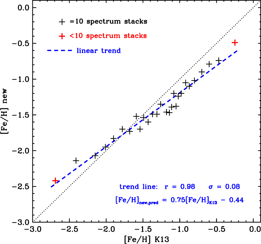
Figure 2: Comparison of metallicities from co-added K13 spectra and the mean values derived in the original K13 analyses. The dotted line represents equality of the [Fe/H] values. The blue dashed line represents the linear regression line through the data; its parameters are entered in the figure.

Figure 4: Correlations of [Fe/H] metallicity (panel a) and [Ba/H] abundances (panel b) in $\delta$ Scuti stars. In panel (a) the dotted line represents the solar value, [Fe/H] = 0, and the dashed line represents the mean of the data points, [Fe/H] = $+$0.12. In panel (b) the dashed line shows a linear regression through the data with the exclusion of the anomalous values for HD 176643 ($v$sin$i$ = 27 km s^-1, [Ba/H] = 2.2) and HD 73798 ($v$sin$i$ = 200 km s^-1, [Ba/H] = 1.0). These data were taken from Ishikawa (1975), Mittermayer & Weiss (2003), Yushchenko et al. (2005), Fossati et al. (2008a, b), Balona et al. (2011), Catanzaro & Ripepi (2014), Escorza et al. (2016), and Joshi et al. (2017).

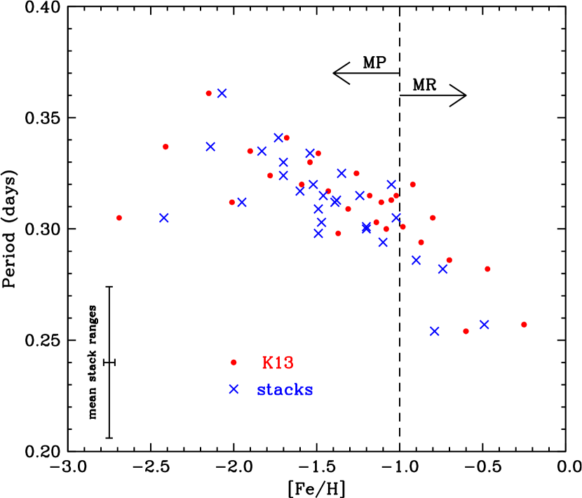
Figure 6: Pulsational period plotted as a function of [Fe/H] metallicity for our stacked spectra. The red dots are K13 values and the blue crosses are from the present study (Table 2. The black dashed line represents the division adpoted in the paper betwee metal-rich (MR) and metal-poor (MP) stars. The mean stack ranges drawn with black solid lines represents mean ranges of [Fe/H] and period in a single stack.

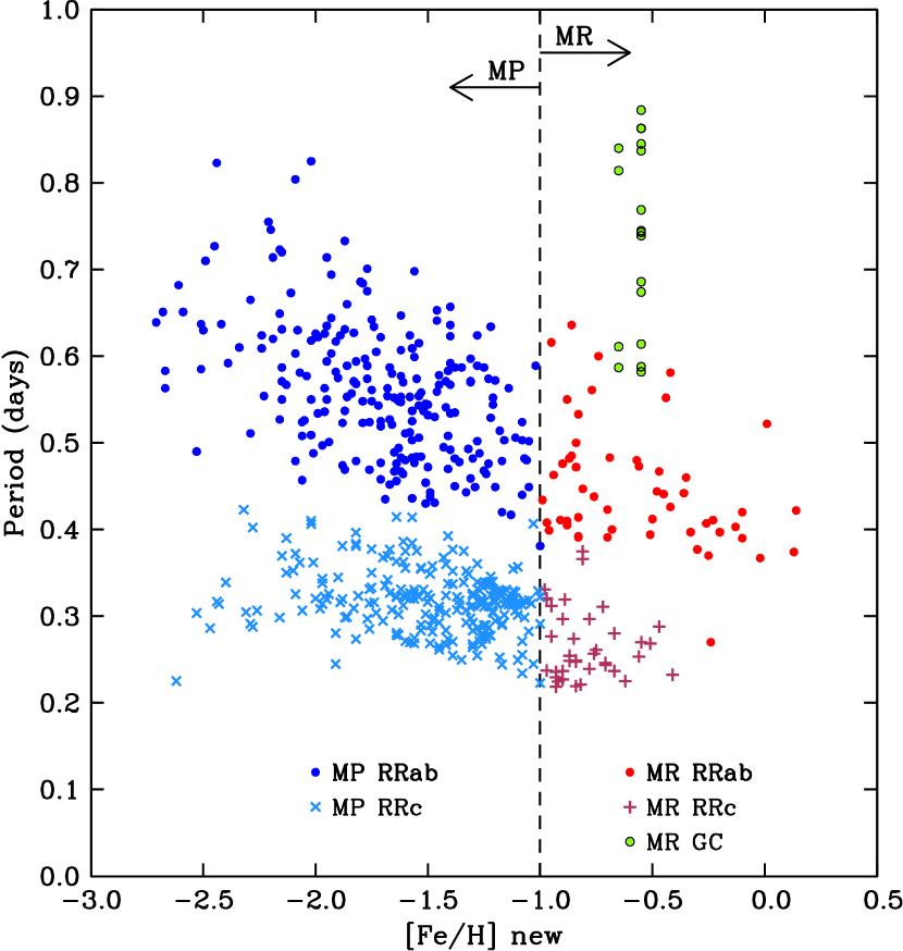
Figure 7: Correlation of RR Lyrae pulsational periods with [Fe/H] metallicities for our RRc stars and the RRab stars of Layden (1994, 1995a). This figure adds our program RRc stars (Table 1) to the RRab stars shown in Figure 1 of Layden (1995a), later adapted as Figure 1 of Chadid et al. (2017). The point types and colors are given in the figure legend. The axis label “[Fe/H] new” means that the RRc metallicities are those of this paper, and the RRab metallicities are those of Layden (1994) rescaled by Chadid et al. (2017). The points for globular clusters (GC) are those of NGC 6388 and NGC 6441, two anomalous MR clusters with very extended horizontal branches (Rich et al., 1997); their [Fe/H] values are unchanged.. The division between metal-poor (MP) and metal-rich (MR) stars at [Fe/H] = $-$1.0 is as in Figure 6. See the text for more discussion of the metallicity scales.

Table 1: RRc Program Stars

Star Name	$P$ (d)	$HJD_{0}$ (d)	$V_{max}$	$V_{amp}$	$S/N$	[Fe/H]	stack #
ASAS	ASAS	ASAS	ASAS	ASAS	K13	K13
124115-4056.9	0.232417	1871.657	12.18	0.35	9.9	$+$0.04	1
012052+2143.7	0.287790	2626.416	10.81	0.37	8.2	$-$0.04	1
095845-5927.8	0.268609	1869.479	11.88	0.50	12.4	$-$0.10	no
141107-4212.2	0.269753	1888.518	12.40	0.41	8.7	$-$0.15	1
195123+0835.0	0.253592	2383.449	10.55	0.11	20.3	$-$0.16	no
054810-2001.4	0.225147	1869.255	8.16	0.34	25.6	$-$0.24	no
210841-5509.1	0.280250	1871.323	13.36	0.54	9.5	$-$0.31	1
045648+1818.3	0.236865	2622.164	11.54	0.37	22.4	$-$0.31	1
185248-5113.8	0.246210	1965.345	13.26	0.39	12.8	$-$0.36	1
042421+0048.8	0.243670	1929.411	12.47	0.31	21.9	$-$0.36	1
203145-2158.7	0.310712	1874.096	11.27	0.37	13.7	$-$0.38	2
083947+1417.4	0.260931	2623.553	11.64	0.37	18.4	$-$0.41	2
071045+1059.2	0.256969	2387.941	12.73	0.39	16.0	$-$0.43	2
082955-6434.6	0.239448	1869.325	12.15	0.57	16.2	$-$0.45	2
224249-7430.3	0.296880	1870.379	11.92	0.18	16.4	$-$0.46	2
143814-4025.6	0.374705	1904.010	13.11	0.53	14.9	$-$0.49	2
192436+0631.4	0.366142	2185.100	12.25	0.54	9.7	$-$0.49	2
115116-5548.3	0.221350	1873.407	10.17	0.36	24.1	$-$0.51	2
182240-4242.9	0.247590	1948.606	12.72	0.36	17.1	$-$0.53	2
175613-4346.3	0.249139	1948.575	11.10	0.47	13.4	$-$0.54	2
175845-5516.4	0.219404	1940.512	11.76	0.35	19.9	$-$0.54	3
045815-2244.5	0.274048	1869.539	12.11	0.41	15.2	$-$0.55	3
155552-2148.6	0.254144	1920.296	11.38	0.44	24.1	$-$0.57	3
185644-3622.6	0.248500	1948.350	9.89	0.38	18.2	$-$0.58	3
121553-5157.4_2	0.319399	1871.920	12.25	0.43	15.5	$-$0.60	3
142032-1432.0	0.296683	1903.631	12.76	0.42	18.9	$-$0.61	3
164410-0112.6	0.227060	1936.644	13.31	0.44	20.1	$-$0.61	3
164128-1029.6	0.236743	1938.338	12.59	0.45	8.4	$-$0.62	3
211058-2140.7	0.224800	1873.283	10.26	0.13	10.0	$-$0.64	3
132225-2042.3	0.235934	1886.414	10.72	0.40	30.5	$-$0.65	3
081012-2903.0	0.229656	1869.397	9.53	0.28	35.9	$-$0.65	4
095438-6240.5	0.218941	1869.191	12.27	0.54	15.8	$-$0.66	4
221135-4222.3	0.311920	1871.329	13.13	0.50	10.7	$-$0.68	4
234439-0148.6	0.276854	1869.174	12.23	0.38	4.9	$-$0.68	4

(This table is available in its entirety in machine-readable form.)

Table 2: Comparison with K13

stack#	count	[Fe/H]	$\Delta$[Fe/H]	[Fe/H]	Teff	log g	$\xi_{\rm t}$	$\langle P\rangle$
		K13	K13	new	new	new	km s-1,new	d
1	7	-0.25	0.40	-0.49	6950	2.6	3.2	0.2567
2	10	-0.47	0.16	-0.74	7000	2.4	3.1	0.2824
3	10	-0.60	0.11	-0.79	7150	2.7	3.3	0.2537
4	10	-0.70	0.10	-0.90	7150	2.3	3.1	0.2859
5	10	-0.80	0.10	-1.02	7100	2.8	3.0	0.3049
6	10	-0.87	0.04	-1.10	7050	2.4	3.0	0.2940
7	10	-0.92	0.07	-1.05	7150	2.6	3.3	0.3198
8	10	-0.98	0.04	-1.20	7000	2.6	3.0	0.3006
9	10	-1.02	0.04	-1.24	7000	2.8	3.0	0.3145
10	10	-1.05	0.02	-1.38	6900	2.5	3.0	0.3127
11	10	-1.08	0.02	-1.20	7000	2.3	2.2	0.2996
12	10	-1.11	0.03	-1.39	6900	2.4	3.0	0.3116
13	10	-1.14	0.01	-1.47	6850	2.2	2.5	0.3031
14	10	-1.18	0.05	-1.46	6900	2.2	2.9	0.3153
15	10	-1.26	0.07	-1.35	7100	2.5	2.8	0.3246
16	10	-1.31	0.05	-1.49	7100	2.4	2.6	0.3086
17	10	-1.37	0.06	-1.49	6950	2.7	2.4	0.2981
18	10	-1.43	0.05	-1.60	6900	2.6	2.6	0.3169
19	10	-1.49	0.05	-1.54	6900	2.8	2.8	0.3337
20	10	-1.54	0.04	-1.70	7000	2.7	3.0	0.3304
21	10	-1.59	0.05	-1.52	7100	2.7	2.2	0.3200
22	10	-1.68	0.10	-1.73	7100	2.6	2.8	0.3410
23	10	-1.78	0.10	-1.70	7100	3.1	2.5	0.3236
24	10	-1.90	0.10	-1.83	7100	2.9	2.2	0.3347
25	10	-2.01	0.10	-1.95	7100	2.9	2.4	0.3123
26	10	-2.15	0.17	-2.07	6900	2.9	1.6	0.3607
27	10	-2.41	0.35	-2.14	7000	2.8	1.8	0.3372
28	4	-2.69	0.14	-2.42	7000	1.9	2.0	0.3052

References

- Antonello et al. (1986) Antonello, E., Broglia, P., Conconi, P., & Mantegazza, L. 1986, A&A, 169, 122
- Balona et al. (2011) Balona, L. A., Ripepi, V., Catanzaro, G., et al. 2011, MNRAS, 414, 792
- Butler (1975) Butler, D. 1975, ApJ, 200, 68
- Butler et al. (1982) Butler, D., Manduca, A., Bell, R. A., & Deming, D. 1982, AJ, 87, 640
- Catanzaro & Ripepi (2014) Catanzaro, G., & Ripepi, V. 2014, MNRAS, 441, 1669
- Chadid et al. (2017) Chadid, M., Sneden, C., & Preston, G. W. 2017, ApJ, 835, 187
- Clementini et al. (1995) Clementini, G., Carretta, E., Gratton, R., et al. 1995, AJ, 110, 2319
- Den Hartog et al. (2014) Den Hartog, E. A., Ruffoni, M. P., Lawler, J. E., et al. 2014, ApJS, 215, 23
- Escorza et al. (2016) Escorza, A., Zwintz, K., Tkachenko, A., et al. 2016, A&A, 588, A71
- Feast et al. (2008) Feast, M. W., Laney, C. D., Kinman, T. D., van Leeuwen, F., & Whitelock, P. A. 2008, MNRAS, 386, 2115
- Fernley & Barnes (1996) Fernley, J., & Barnes, T. G. 1996, A&A, 312, 957
- Fernley et al. (1990) Fernley, J. A., Skillen, I., Jameson, R. F., & Longmore, A. J. 1990, MNRAS, 242, 685
- For et al. (2011a) For, B.-Q., Preston, G. W., & Sneden, C. 2011a, ApJS, 194, 38
- For et al. (2011b) For, B.-Q., Sneden, C., & Preston, G. W. 2011b, ApJS, 197, 29
- Fossati et al. (2008a) Fossati, L., Bagnulo, S., Landstreet, J., et al. 2008a, A&A, 483, 891
- Fossati et al. (2008b) Fossati, L., Kolenberg, K., Reegen, P., & Weiss, W. 2008b, A&A, 485, 257
- Govea et al. (2014) Govea, J., Gomez, T., Preston, G. W., & Sneden, C. 2014, ApJ, 782, 59
- Ishikawa (1975) Ishikawa, M. 1975, PASJ, 27, 1
- Jones et al. (1988) Jones, R. V., Carney, B. W., & Latham, D. W. 1988, ApJ, 326, 312
- Joshi et al. (2017) Joshi, S., Semenko, E., Moiseeva, A., et al. 2017, MNRAS, 467, 633
- Kelson (2003) Kelson, D. D. 2003, PASP, 115, 688
- Kollmeier et al. (2013) Kollmeier, J. A., Szczygieł, D. M., Burns, C. R., et al. 2013, ApJ, 775, 57
- Kramida et al. (2015) Kramida, A., Yu. Ralchenko, Reader, J., & and NIST ASD Team. 2015, NIST Atomic Spectra Database (ver. 5.3), [Online]. Available: http://physics.nist.gov/asd [2017, May 12]. National Institute of Standards and Technology, Gaithersburg, MD.
- Kurucz (2011) Kurucz, R. L. 2011, Canadian Journal of Physics, 89, 417
- Lambert et al. (1996) Lambert, D. L., Heath, J. E., Lemke, M., & Drake, J. 1996, ApJS, 103, 183
- Lawler et al. (2013) Lawler, J. E., Guzman, A., Wood, M. P., Sneden, C., & Cowan, J. J. 2013, ApJS, 205, 11
- Layden et al. (2013) Layden, A., Anderson, T., & Husband, P. 2013, ArXiv e-prints, arXiv:1310.0549
- Layden (1994) Layden, A. C. 1994, AJ, 108, 1016
- Layden (1995a) —. 1995a, AJ, 110, 2312
- Layden (1995b) —. 1995b, AJ, 110, 2288
- Liu et al. (2013) Liu, S., Zhao, G., Chen, Y.-Q., Takeda, Y., & Honda, S. 2013, Research in Astronomy and Astrophysics, 13, 1307
- Liu (1991) Liu, T. 1991, PASP, 103, 205
- Liu & Janes (1989) Liu, T., & Janes, K. A. 1989, ApJS, 69, 593
- Marconi et al. (2015) Marconi, M., Coppola, G., Bono, G., et al. 2015, ApJ, 808, 50
- Mittermayer & Weiss (2003) Mittermayer, P., & Weiss, W. W. 2003, A&A, 407, 1097
- Nemec et al. (2013) Nemec, J. M., Cohen, J. G., Ripepi, V., et al. 2013, ApJ, 773, 181
- O’Brian et al. (1991) O’Brian, T. R., Wickliffe, M. E., Lawler, J. E., Whaling, W., & Brault, J. W. 1991, Journal of the Optical Society of America B Optical Physics, 8, 1185
- Pancino et al. (2015) Pancino, E., Britavskiy, N., Romano, D., et al. 2015, MNRAS, 447, 2404
- Pojmanski (2002) Pojmanski, G. 2002, Acta Astron., 52, 397
- Pojmanski et al. (2005) Pojmanski, G., Pilecki, B., & Szczygiel, D. 2005, Acta Astron., 55, 275
- Preston (1959) Preston, G. W. 1959, ApJ, 130, 507
- Preston (2011) —. 2011, AJ, 141, 6
- Rich et al. (1997) Rich, R. M., Sosin, C., Djorgovski, S. G., et al. 1997, ApJ, 484, L25
- Rodríguez et al. (2000) Rodríguez, E., López-González, M. J., & López de Coca, P. 2000, A&AS, 144, 469
- Ruffoni et al. (2014) Ruffoni, M. P., Den Hartog, E. A., Lawler, J. E., et al. 2014, MNRAS, 441, 3127
- Smith (1995) Smith, H. A. 1995, Cambridge Astrophysics Series, 27
- Sneden (1973) Sneden, C. 1973, ApJ, 184, 839
- Sneden et al. (2016) Sneden, C., Cowan, J. J., Kobayashi, C., et al. 2016, ApJ, 817, 53
- Sneden et al. (2017) Sneden, C., Preston, G. W., & Chadid, M. 2017, ApJ, in press
- Szczygieł & Fabrycky (2007) Szczygieł, D. M., & Fabrycky, D. C. 2007, MNRAS, 377, 1263
- Szczygieł et al. (2009) Szczygieł, D. M., Pojmański, G., & Pilecki, B. 2009, Acta Astron., 59, 137
- Tody (1993) Tody, D. 1993, in Astronomical Society of the Pacific Conference Series, Vol. 52, Astronomical Data Analysis Software and Systems II, ed. R. J. Hanisch, R. J. V. Brissenden, & J. Barnes, 173
- Wood et al. (2013) Wood, M. P., Lawler, J. E., Sneden, C., & Cowan, J. J. 2013, ApJS, 208, 27
- Yushchenko et al. (2005) Yushchenko, A., Gopka, V., Kim, C., et al. 2005, MNRAS, 359, 865
- Zacharias et al. (2013) Zacharias, N., Finch, C. T., Girard, T. M., et al. 2013, AJ, 145, 44
- Zacharias et al. (2004) Zacharias, N., Urban, S. E., Zacharias, M. I., et al. 2004, AJ, 127, 3043
- Zinn & West (1984) Zinn, R., & West, M. J. 1984, ApJS, 55, 45