Strong and uniform convergence in the teleportation simulation of
bosonic Gaussian channels

Abstract

In the literature on the continuous-variable bosonic teleportation protocol due to [Braunstein and Kimble, Phys. Rev. Lett., 80(4):869, 1998], it is often loosely stated that this protocol converges to a perfect teleportation of an input state in the limit of ideal squeezing and ideal detection, but the exact form of this convergence is typically not clarified. In this paper, I explicitly clarify that the convergence is in the strong sense, and not the uniform sense, and furthermore, that the convergence occurs for any input state to the protocol, including the infinite-energy Basel states defined and discussed here. I also prove, in contrast to the above result, that the teleportation simulations of pure-loss, thermal, pure-amplifier, amplifier, and additive-noise channels converge both strongly and uniformly to the original channels, in the limit of ideal squeezing and detection for the simulations. For these channels, I give explicit uniform bounds on the accuracy of their teleportation simulations. I then extend these uniform convergence results to particular multi-mode bosonic Gaussian channels. These convergence statements have important implications for mathematical proofs that make use of the teleportation simulation of bosonic Gaussian channels, some of which have to do with bounding their non-asymptotic secret-key-agreement capacities. As a byproduct of the discussion given here, I confirm the correctness of the proof of such bounds from my joint work with Berta and Tomamichel from [Wilde, Tomamichel, Berta, IEEE Trans. Inf. Theory 63(3):1792, March 2017]. Furthermore, I show that it is not necessary to invoke the energy-constrained diamond distance in order to confirm the correctness of this proof.

I Introduction

The quantum teleportation protocol is one of the most powerful primitives in quantum information theory PhysRevLett.70.1895 . By sharing entanglement and making use of a classical communication link, a sender can transmit an arbitrary quantum state to a receiver. In resource-theoretic language, the resources of a maximally entangled state of two qubits

$$|\Phi^{+}\rangle_{AB}=(|00\rangle_{AB}+|11\rangle_{AB})/\sqrt{2}$$ (1)

and two classical bit channels can be used to simulate an ideal qubit channel from the sender to the receiver Bennett04 ; DHW05RI . Generalizing this, a maximally entangled state of two qudits

$$|\Phi_{d}\rangle_{AB}=d^{-1/2}\sum_{i=0}^{d-1}|i\rangle_{A}|i\rangle_{B}$$ (2)

and two classical channels, each of dimension $d$, can be used to simulate an ideal $d$-dimensional quantum channel PhysRevLett.70.1895 . The teleportation primitive has been extended in multiple non-trivial ways, including a method to simulate an unideal channel using a noisy, mixed resource state (BDSW96, , Section V) (see also HHH99 ; WPG07 ; NFC09 ; Mul12 ) and as a way to implement nonlocal quantum gates GC99 ; STM11 . The former extension has been used to bound the rates at which quantum information can be conveyed over a quantum channel assisted by local operations and classical communication (LOCC) BDSW96 ; Mul12 , and more generally, as a way to reduce a general LOCC-assisted protocol to one that consists of preparing a resource state followed by a single round of LOCC BDSW96 ; Mul12 .

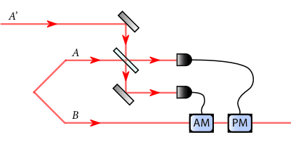
Figure 1: Depiction of the bosonic continuous-variable teleportation protocol from prl1998braunstein , described in the main text. “AM” and “PM” denote amplitude and phase modulators, which implement the displacement operator needed in the teleportation protocol.

Due in part to the large experimental interest in bosonic continuous-variable quantum systems, given their practical applications adesso14 ; S17 , the teleportation protocol was extended to this paradigm prl1998braunstein (see Figure 1). The standard protocol begins with a sender and receiver sharing a two-mode squeezed vacuum state of the following form:

$$|\Phi(N_{S})\rangle_{AB}\equiv\frac{1}{\sqrt{N_{S}+1}}\sum_{n=0}^{\infty}\left(\sqrt{\frac{N_{S}}{N_{S}+1}}\right)^{n}|n\rangle_{A}|n\rangle_{B},$$ (3)

where $N_{S}\in[0,\infty)$ represents the squeezing strength and $\{|n\rangle\}_{n}$ denotes the photon-number basis. Suppose that the goal is to teleport a mode $A^{\prime}$. The sender mixes, on a 50-50 beamsplitter, the mode $A^{\prime}$ with the mode $A$ of the state in (3). Afterward, the sender performs homodyne detection on the modes emerging from the beamsplitter and forwards the measurement results over classical channels to the receiver, who possesses mode $B$ of the above state. Finally, the receiver performs a unitary displacement operation on mode $B$. In the limit as $N_{S}\rightarrow\infty$ and in the limit of ideal homodyne detection, this continuous-variable teleportation protocol is often loosely stated in the literature to simulate an ideal channel on any state of the mode $A^{\prime}$, such that this state is prepared in mode $B$ after the protocol is finished. Due to the lack of a precise notion of convergence being given, there is the potential for confusion regarding mathematical proofs that make use of the continuous-variable teleportation protocol.

With this in mind, one purpose of the present paper is to clarify the precise kind of convergence that occurs in continuous-variable quantum teleportation, which is typically not discussed in the literature on this topic. In particular, I prove that the convergence is in the strong topology sense, and not in the uniform topology sense (see, e.g., (SH08, , Section 3) for discussions of these notions of convergence). I then show how to extend this strong convergence result to the teleportation simulation of $n$ parallel ideal channels, and I also show how this strong convergence extends to the teleportation simulation of $n$ ideal channels that could be used in any context.

Strong convergence and uniform convergence are then discussed for the teleportation simulation of bosonic Gaussian channels. For this latter case, and in contrast to the result discussed above for the continuous-variable teleportation protocol, I prove that the teleportation simulations of the pure-loss, thermal, pure-amplifier, amplifier, and additive-noise channels converge both strongly and uniformly to the original channels, in the limit of ideal squeezing and detection for the simulations. Here I give explicit uniform bounds on the accuracy of the teleportation simulations of these channels, and I suspect that these bounds will be useful in future applications. After this development, I then extend these uniform convergence results to particular multi-mode bosonic Gaussian channels.

These convergence results are important, even if they might be implicit in prior works, as they provide meaningful clarification of mathematical proofs that make use of teleportation simulation, such as those given in recent work on bounding non-asymptotic secret-key-agreement capacities. In particular, one can employ these convergence statements to confirm the correctness of the proof of such bounds given in my joint work with Berta and Tomamichel from WTB16 . Furthermore, these strong convergence statements can be used to conclude that the energy-constrained diamond distance is not necessary to arrive at a proof of the bounds from WTB16 . Another byproduct of the discussion given in the present paper is that it is clarified that the methods of WTB16 allow for bounding secret-key rates of rather general protocols that make use of infinite-energy states, such as the Basel states in (20) and (124). Although there should be great skepticism concerning whether these infinite-energy Basel states could be generated in practice, this latter byproduct is nevertheless of theoretical interest.

The rest of the paper proceeds as follows. In the next section, I discuss the precise form of convergence that occurs in continuous-variable quantum teleportation and then develop various extensions of this notion of convergence. I then prove that teleportation simulations of the pure-loss, thermal, pure-amplifier, amplifier, and additive-noise channels converge both strongly and uniformly to the original channels in the limit of ideal squeezing and detection for the simulations. The uniform convergence results are then extended to the teleportation simulations of particular multi-mode bosonic Gaussian channels. Section III gives a physical interpretation of the aforementioned convergence results, by means of the CV Teleportation Game. After that, Section IV briefly reviews what is meant by a secret-key-agreement protocol and non-asymptotic secret-key-agreement capacity. Finally, in Section V, I review the proof of (WTB16, , Theorem 24) and carefully go through some of its steps therein, confirming its correctness, while showing how the strong convergence of teleportation simulation applies. In Section VI, I conclude with a brief summary and a discussion.

II Notions of quantum channel convergence, with applications to teleportation simulation

One main technical issue discussed in this paper is how the continuous-variable bosonic teleportation protocol from prl1998braunstein  converges to an identity channel in the limit of infinite squeezing and ideal detection. This issue is often not explicitly clarified in the literature on the topic, even though it has been implicit for some time in various works that the convergence is to be understood in the strong sense (topology of strong convergence), and not necessarily the uniform sense (topology of uniform convergence) (see, e.g., (SH08, , Section 3)). For example, in the original paper prl1998braunstein , the following statement is given regarding this issue:

“Clearly, for $r\rightarrow\infty$ the teleported state of Eq. (4) reproduces the original unknown state.”

Although it is clear that this statement implies convergence in the strong sense, it could be helpful to clarify this point, and the purpose of this section is to do so.

In what follows, I first recall the definitions of strong and uniform convergence from (SH08, , Section 3). I then discuss the precise form of convergence that occurs in continuous-variable bosonic teleportation and show how strong convergence and uniform convergence are extremely different in the setting of continuous-variable teleportation. After that, I prove that strong convergence of a channel sequence implies strong convergence of $n$-fold tensor powers of these channels and follow this with a proof that strong convergence of a channel sequence implies strong convergence of $n$ uses of these channels in any context in which they could be invoked. I also prove that the teleportation simulations of pure-loss, thermal, pure-amplifier, amplifier, and additive-noise channels converge both strongly and uniformly to the original channels, in the limit of ideal squeezing and detection for the simulations. The uniform convergence results are then extended to the teleportation simulations of particular multi-mode bosonic Gaussian channels.

II.1 Definitions of strong and uniform convergence

Before discussing the precise statement of convergence in the continuous-variable bosonic teleportation protocol, let us begin by recalling general definitions of strong and uniform convergence from (SH08, , Section 3). I adopt slightly different definitions from those given in (SH08, , Section 3), in order to suit the needs of the present paper, but note that they are equivalent to the original definitions as shown in SH08 and (Sh17, , Lemma 2). In this context, see also Sh17a . Let $\{\mathcal{N}_{A\rightarrow B}^{k}\}_{k}$ denote a sequence of quantum channels (completely positive, trace-preserving maps), which each accept as input a trace-class operator acting on a separable Hilbert space $\mathcal{H}_{A}$ and output a trace-class operator acting on a separable Hilbert space $\mathcal{H}_{B}$. This sequence converges strongly to a channel $\mathcal{N}_{A\rightarrow B}$ if for all density operators $\rho_{RA}$ acting on $\mathcal{H}_{R}\otimes\mathcal{H}_{A}$, where $\mathcal{H}_{R}$ is an arbitrary, auxiliary separable Hilbert space, the following limit holds

$$\lim_{k\rightarrow\infty}\varepsilon(k,\rho_{RA})=0,$$ (4)

where the infidelity is defined as

$$\varepsilon(k,\rho_{RA})\equiv\\ 1-F((\operatorname{id}_{R}\otimes\mathcal{N}_{A\rightarrow B}^{k})(\rho_{RA}),(\operatorname{id}_{R}\otimes\mathcal{N}_{A\rightarrow B})(\rho_{RA})),$$ (5)

$\operatorname{id}_{R}$ denotes the identity map on the auxiliary space, and $F(\tau,\omega)\equiv\left\|\sqrt{\tau}\sqrt{\omega}\right\|_{1}^{2}$ is the quantum fidelity U76 , defined for density operators $\tau$ and $\omega$. The quantum fidelity obeys a data processing inequality, which is the statement that

$$F(\mathcal{M}(\tau),\mathcal{M}(\omega))\geq F(\tau,\omega),$$ (6)

for states $\tau$ and $\omega$ and a quantum channel $\mathcal{M}$. We can summarize strong convergence more compactly as the following mathematical statement:

$$\sup_{\rho_{RA}}\lim_{k\rightarrow\infty}\varepsilon(k,\rho_{RA})=0.$$ (7)

Due to purification, the Schmidt decomposition theorem, and the data processing inequality for fidelity, we find that for every mixed state $\rho_{RA}$, there exists a pure state $\psi_{R^{\prime}A}$ with the auxiliary Hilbert space $\mathcal{H}_{R^{\prime}}$ taken to be isomorphic to $\mathcal{H}_{A}$, such that

$$\varepsilon(k,\rho_{RA})\leq\varepsilon(k,\psi_{R^{\prime}A}).$$ (8)

Thus, when considering strong convergence, it suffices to consider only pure states $\psi_{R^{\prime}A}$, so that

$$\sup_{\rho_{RA}}\lim_{k\rightarrow\infty}\varepsilon(k,\rho_{RA})=\sup_{\psi_{R^{\prime}A}}\lim_{k\rightarrow\infty}\varepsilon(k,\psi_{R^{\prime}A}).$$ (9)

Strong convergence is strictly different from uniform convergence (SH08, , Section 3), which amounts to a swap of the supremum and the limit in (7). That is, the channel sequence $\{\mathcal{N}_{A\rightarrow B}^{k}\}_{k}$ converges uniformly to the channel $\mathcal{N}_{A\rightarrow B}$ if the following holds

$$\lim_{k\rightarrow\infty}\sup_{\rho_{RA}}\varepsilon(k,\rho_{RA})=0.$$ (10)

Even though this swap might seem harmless and is of no consequence in finite dimensions, the issue is important to consider in infinite-dimensional contexts, especially for bosonic channels. That is, a sequence of channels could converge in the strong sense, but be as far as possible from converging in the uniform sense, and an example of this behavior is given in the next subsection.

It was also stressed in SH08 that the topology of uniform convergence is too strong for physical applications and should typically not be considered.

II.2 Strong and uniform convergence considerations for continuous-variable teleportation

We now turn our attention to convergence in the continuous-variable bosonic teleportation protocol and focus on (prl1998braunstein, , Eq. (9)), which states that an unideal continuous-variable bosonic teleportation protocol with input mode$~{}A$ realizes the following additive-noise quantum Gaussian channel $\mathcal{T}_{A}^{\bar{\sigma}}$ on an input density operator $\rho_{A}$:

$$\rho_{A}\rightarrow\mathcal{T}_{A}^{\bar{\sigma}}(\rho_{A})\equiv\int d^{2}\alpha\ G_{\bar{\sigma}}(\alpha)\ D(\alpha)\rho_{A}D(-\alpha),$$ (11)

where $D(\alpha)$ is a displacement operator S17 and

$$G_{\bar{\sigma}}(\alpha)\equiv\frac{1}{\pi\bar{\sigma}}\exp\!\left(-\frac{\left|\alpha\right|^{2}}{\bar{\sigma}}\right)$$ (12)

is a zero-mean, circularly symmetric complex Gaussian probability density function with variance $\bar{\sigma}>0$. To be clear, the integral in (11) is over the whole complex plane $\alpha\in\mathbb{C}$. For an explicit proof of (11), one can also consult TBS02 ; BST02 . The variance parameter $\bar{\sigma}$ quantifies unideal squeezing and unideal detection. Thus, for any $\bar{\sigma}>0$, the teleportation channel $\mathcal{T}_{A}^{\bar{\sigma}}$ is unideal and intuitively becomes ideal in the limit $\bar{\sigma}\rightarrow 0$. However, it is this convergence that needs to be made precise. To examine this, we need a measure of the channel input-output dissimilarity, and the entanglement infidelity is a good choice, which is essentially the choice made in prl1998braunstein for quantifying the performance of unideal bosonic teleportation. For a fixed pure state $\psi_{RA}\equiv|\psi\rangle\langle\psi|_{RA}$ of modes $R$ and $A$, the entanglement infidelity of the channel $\mathcal{T}_{A}^{\bar{\sigma}}$ with respect to $\psi_{RA}$ is defined as

$$\varepsilon(\bar{\sigma},\psi_{RA})\equiv 1-\langle\psi|_{RA}(\operatorname{id}_{R}\otimes\mathcal{T}_{A}^{\bar{\sigma}})(|\psi\rangle\langle\psi|_{RA})|\psi\rangle_{RA}.$$ (13)

Examining (prl1998braunstein, , Eq. (11)), we see that the entanglement infidelity can alternatively be written as

$$\varepsilon(\bar{\sigma},\psi_{RA})=1-\int d^{2}\alpha\ G_{\bar{\sigma}}(\alpha)\left|\chi_{\psi_{A}}(\alpha)\right|^{2},$$ (14)

where $\chi_{\psi_{A}}(\alpha)=\operatorname{Tr}\{D(\alpha)\psi_{A}\}$ is the Wigner characteristic function of the reduced density operator $\psi_{A}$. By applying the Hölder inequality, we conclude that $\chi_{\psi_{A}}(\alpha)$ is bounded for all $\alpha\in\mathbb{C}$ because

$$\left|\operatorname{Tr}\{D(\alpha)\psi_{A}\}\right|\leq\left\|D(\alpha)\right\|_{\infty}\left\|\psi_{A}\right\|_{1}=1.$$ (15)

Exploiting the continuity of $\chi_{\psi_{A}}(\alpha)$ at $\alpha=0$ and the fact that $\chi_{\psi_{A}}(0)=1$ (Hol11, , Theorem 5.4.1), as well as invoking the boundedness of $\chi_{\psi_{A}}(\alpha)$ and (WZ77, , Theorem 9.8) regarding the convergence of nascent delta functions, we then conclude that for a given state $\psi_{RA}$, the following strong convergence holds

$$\lim_{\bar{\sigma}\rightarrow 0}\varepsilon(\bar{\sigma},\psi_{RA})=0,$$ (16)

which can be written, as before, more compactly as

$$\sup_{\psi_{RA}}\lim_{\bar{\sigma}\rightarrow 0}\varepsilon(\bar{\sigma},\psi_{RA})=0.$$ (17)

Note that, as before and due to (9), Eq. (17) implies that

$$\sup_{\rho_{RA}}\lim_{\bar{\sigma}\rightarrow 0}\varepsilon(\bar{\sigma},\rho_{RA})=0$$ (18)

for any mixed state $\rho_{RA}$ where

$$\varepsilon(\bar{\sigma},\rho_{RA})\equiv 1-F(\rho_{RA},(\operatorname{id}_{R}\otimes\mathcal{T}_{A}^{\bar{\sigma}})(\rho_{RA}))$$ (19)

and $\mathcal{H}_{R}$ is an arbitrary auxiliary separable Hilbert space.

One should note here that the convergence in (17) already calls into question any claim regarding the necessity of an energy constraint for the states that are to be teleported using the continuous-variable teleportation protocol. Clearly, the state $\psi_{RA}$ to be teleported could be chosen as the following Basel state:

$$|\beta\rangle_{RA}=\sqrt{\frac{6}{\pi^{2}}}\sum_{n=1}^{\infty}\sqrt{\frac{1}{n^{2}}}|n\rangle_{R}|n\rangle_{A},$$ (20)

which has mean photon number equal to $\infty$, but it also satisfies (16). Such a state is called a “Basel state,” due to its normalization factor being connected with the well known Basel problem, which establishes that $\sum_{n=1}^{\infty}1/n^{2}=\pi^{2}/6$. For $\hat{n}=\sum_{n=0}^{\infty}n|n\rangle\langle n|$ the photon-number operator, one can easily check that the mean photon number $\operatorname{Tr}\{(\hat{n}_{R}+\hat{n}_{A})\beta_{RA}\}=\infty$, due to the presence of the divergent harmonic series after $\hat{n}_{A}$ multiplies the reduced density operator $\beta_{A}$. Thus, the only constraint needed for the convergence in (17) is that the state to be teleported be a state (i.e., normalizable). Ref. P17 claims that it is necessary for there to be an energy constraint for strong convergence in teleportation; however, the example of the Basel states given above proves that such an energy constraint is not necessary.

It is also important to note that an exchange of the limit and the supremum in (17) leads to a drastically different conclusion:

$$\lim_{\bar{\sigma}\rightarrow 0}\sup_{\psi_{RA}}\varepsilon(\bar{\sigma},\psi_{RA})=1.$$ (21)

The drastic difference is due to the fact that for all fixed $\bar{\sigma}>0$, one can find a sequence of states $\{\psi_{RA}^{k}\}_{k}$ such that $\sup_{k}\varepsilon(\bar{\sigma},\psi_{RA}^{k})=1$, establishing (21). For example, one could pick each $\psi_{RA}^{k}$ to be a two-mode squeezed vacuum state with squeezing parameter increasing with increasing $k$. In the limit of large squeezing, the ideal channel and the additive-noise channel for any $\bar{\sigma}>0$ become perfectly distinguishable, having infidelity approaching one, implying (21). One can directly verify this calculation by employing the covariance matrix representation of the two-mode squeezed vacuum and the additive-noise channel, as well as the overlap formula in (S17, , Eq. (4.51)) to calculate entanglement fidelity.

I now give details of the aforementioned calculation, regarding how the continuous-variable bosonic teleportation protocol from prl1998braunstein does not converge uniformly to an ideal channel. Consider a two-mode squeezed vacuum state $\Phi(N_{S})$ with mean photon number $N_{S}$ for one of its reduced modes, as defined in (3). Such a state has a Wigner-function covariance matrix S17  as follows:

$$\begin{bmatrix}2N_{S}+1&2\sqrt{N_{S}(N_{S}+1)}\\ 2\sqrt{N_{S}(N_{S}+1)}&2N_{S}+1\end{bmatrix}\\ \oplus\begin{bmatrix}2N_{S}+1&-2\sqrt{N_{S}(N_{S}+1)}\\ -2\sqrt{N_{S}(N_{S}+1)}&2N_{S}+1\end{bmatrix}.$$ (22)

After sending one mode of this state through an additive-noise channel with variance $\bar{\sigma}$ (corresponding to an unideal continuous-variable bosonic teleportation), the covariance matrix becomes as follows, corresponding to a state $\tau(N_{S},\bar{\sigma})$:

$$\begin{bmatrix}2N_{S}+1&2\sqrt{N_{S}(N_{S}+1)}\\ 2\sqrt{N_{S}(N_{S}+1)}&2N_{S}+1+2\bar{\sigma}\end{bmatrix}\\ \oplus\begin{bmatrix}2N_{S}+1&-2\sqrt{N_{S}(N_{S}+1)}\\ -2\sqrt{N_{S}(N_{S}+1)}&2N_{S}+1+2\bar{\sigma}\end{bmatrix}.$$ (23)

The overlap $\operatorname{Tr}\{\omega\sigma\}$ of two zero-mean, two-mode Gaussian states $\omega$ and $\sigma$ is given by (S17, , Eq. (4.51))

$$\operatorname{Tr}\{\omega\sigma\}=4/\sqrt{\det(V_{\omega}+V_{\sigma})},$$ (24)

where $V_{\omega}$ and $V_{\sigma}$ are the Wigner-function covariance matrices of $\omega$ and $\sigma$, respectively. We can then employ this formula to calculate the overlap

$$\langle\Phi(N_{S})|\tau(N_{S},\bar{\sigma})|\Phi(N_{S})\rangle=\operatorname{Tr}\{\Phi(N_{S})\tau(N_{S},\bar{\sigma})\}$$ (25)

as

$$\langle\Phi(N_{S})|\tau(N_{S},\bar{\sigma})|\Phi(N_{S})\rangle=\frac{1}{\bar{\sigma}+2\bar{\sigma}N_{S}+1}.$$ (26)

Thus, for a fixed $\bar{\sigma}>0$ and in the limit as $N_{S}\rightarrow\infty$, we find that $1-\langle\Phi(N_{S})|\tau(N_{S},\bar{\sigma})|\Phi(N_{S})\rangle\rightarrow 1$, so that the continuous-variable bosonic teleportation protocol from prl1998braunstein  does not converge uniformly to an ideal channel.

To summarize, the kind of convergence considered in (17) is the strong sense (topology of strong convergence), whereas the kind of convergence considered in (21) is the uniform sense (topology of uniform convergence) (see, e.g., (SH08, , Section 3)). That is, (17) demonstrates that unideal continuous-variable bosonic teleportation converges strongly to an ideal quantum channel in the limit of ideal squeezing and detection, whereas (21) demonstrates that it does not converge uniformly.

II.3 Strong and uniform convergence for tensor-power channels

A natural consideration to make in the context of quantum Shannon theory is the convergence of $n$ uses of a channel on a general state of $n$ systems, where $n$ is a positive integer. To this end, suppose that the strong convergence in (7) holds for the sequence $\{\mathcal{N}_{A\rightarrow B}^{k}\}_{k}$ of channels. Then it immediately follows that the sequence $\{(\mathcal{N}_{A\rightarrow B}^{k})^{\otimes n}\}_{k}$ converges strongly to $\mathcal{N}_{A\rightarrow B}^{\otimes n}$. Indeed, for an arbitrary density operator $\rho_{RA^{n}}$ acting on $\mathcal{H}_{R}\otimes\mathcal{H}_{A}^{\otimes n}$, we are now interested in bounding the infidelity for the tensor-power channels $(\mathcal{N}_{A\rightarrow B}^{k})^{\otimes n}$ and $\mathcal{N}_{A\rightarrow B}^{\otimes n}$:

$$\varepsilon^{(n)}(k,\rho_{RA^{n}})\equiv\\ 1-F((\operatorname{id}_{R}\otimes(\mathcal{N}_{A\rightarrow B}^{k})^{\otimes n})(\rho_{RA^{n}}),(\operatorname{id}_{R}\otimes\mathcal{N}_{A\rightarrow B}^{\otimes n})(\rho_{RA^{n}})),$$ (27)

in the limit as $k\rightarrow\infty$. By employing the fact that

$$P(\tau,\omega)\equiv\sqrt{1-F(\tau,\omega)}$$ (28)

obeys the triangle inequality R02 ; R03 ; GLN04 ; R06 , we conclude that, for an arbitrary density operator $\rho_{RA^{n}}$, the following inequality holds

$$P\left[(\operatorname{id}_{R}\otimes(\mathcal{N}_{A\rightarrow B}^{k})^{\otimes n})(\rho_{RA^{n}}),(\operatorname{id}_{R}\otimes\mathcal{N}_{A\rightarrow B}^{\otimes n})(\rho_{RA^{n}})\right]$$

$$\leq\sum_{i=1}^{n}P\left[(\operatorname{id}_{R}\otimes(\mathcal{N}_{A\rightarrow B}^{k})^{\otimes i}\otimes\mathcal{N}_{A\rightarrow B}^{\otimes n-i})(\rho_{RA^{n}}),(\operatorname{id}_{R}\otimes(\mathcal{N}_{A\rightarrow B}^{k})^{\otimes i-1}\otimes\mathcal{N}_{A\rightarrow B}^{\otimes n-i+1})(\rho_{RA^{n}})\right]$$ (29)

$$\leq\sum_{i=1}^{n}P\left[(\operatorname{id}_{R}\otimes\operatorname{id}_{A}^{\otimes i-1}\otimes\mathcal{N}_{A\rightarrow B}^{k}\otimes\mathcal{N}_{A\rightarrow B}^{\otimes n-i})(\rho_{RA^{n}}),(\operatorname{id}_{R}\otimes\operatorname{id}_{A}^{\otimes i-1}\otimes\mathcal{N}_{A\rightarrow B}\otimes\mathcal{N}_{A\rightarrow B}^{\otimes n-i})(\rho_{RA^{n}})\right].$$ (30)

The first inequality follows from the triangle inequality for $P(\tau,\omega)$, and the second follows from data processing for the fidelity under the channel

$$\operatorname{id}_{R}\otimes(\mathcal{N}_{A\rightarrow B}^{k})^{\otimes i-1}\otimes\operatorname{id}_{A}^{\otimes n-i+1}$$ (31)

acting on the states

$$(\operatorname{id}_{R}\otimes\operatorname{id}_{A}^{\otimes i-1}\otimes\mathcal{N}_{A\rightarrow B}^{k}\otimes\mathcal{N}_{A\rightarrow B}^{\otimes n-i})(\rho_{RA^{n}}),$$ (32)

$$(\operatorname{id}_{R}\otimes\operatorname{id}_{A}^{\otimes i-1}\otimes\mathcal{N}_{A\rightarrow B}\otimes\mathcal{N}_{A\rightarrow B}^{\otimes n-i})(\rho_{RA^{n}}).$$ (33)

The method used in (29)–(30) is related to the telescoping approach of LS09 , employed in the context of continuity of quantum channel capacities (see the proof of (LS09, , Theorem 11) in particular). Now employing strong convergence of the channel sequence $\{\mathcal{N}_{A\rightarrow B}^{k}\}_{k}$ and the fact that $\mathcal{N}_{A\rightarrow B}^{\otimes n-i}(\rho_{RA^{n}})$ is a fixed state independent of $k$ for each $i\in\{1,\ldots,n\}$, we conclude that for all density operators $\rho_{RA^{n}}$

$$\lim_{k\rightarrow\infty}\varepsilon^{(n)}(k,\rho_{RA^{n}})=0.$$ (34)

This result can be summarized more compactly as

$$\sup_{\rho_{RA}}\lim_{k\rightarrow\infty}\varepsilon(k,\rho_{RA})=0\\ \Longrightarrow\sup_{\rho_{RA^{n}}}\lim_{k\rightarrow\infty}\varepsilon^{(n)}(k,\rho_{RA^{n}})=0.$$ (35)

That is, the strong convergence of the channel sequence $\{\mathcal{N}_{A\rightarrow B}^{k}\}_{k}$ implies the strong convergence of the tensor-power channel sequence $\{(\mathcal{N}_{A\rightarrow B}^{k})^{\otimes n}\}_{k}$ for any finite $n$.

For the case of continuous-variable teleportation, we have that $n$ unideal teleportations with the same performance corresponds to the tensor-power channel $(\mathcal{T}_{A}^{\bar{\sigma}})^{\otimes n}$. By appealing to (17) and (35), or alternatively employing Wigner characteristic functions, (Hol11, , Theorem 5.4.1), and (WZ77, , Theorem 9.8), the following convergence holds: for a pure state $\psi_{RA^{n}}$, we have that

$$\lim_{\bar{\sigma}\rightarrow 0}\varepsilon^{(n)}(\bar{\sigma},\psi_{RA^{n}})=0,$$ (36)

where

$$\varepsilon^{(n)}(\bar{\sigma},\psi_{RA^{n}})\equiv\\ 1-\langle\psi|_{RA^{n}}(\operatorname{id}_{R}\otimes(\mathcal{T}_{A}^{\bar{\sigma}})^{\otimes n})(|\psi\rangle\langle\psi|_{RA^{n}})|\psi\rangle_{RA^{n}}.$$ (37)

Again, more compactly, this is the same as

$$\sup_{\psi_{RA^{n}}}\lim_{\bar{\sigma}\rightarrow 0}\varepsilon^{(n)}(\bar{\sigma},\psi_{RA^{n}})=0.$$ (38)

and drastically different from

$$\lim_{\bar{\sigma}\rightarrow 0}\sup_{\psi_{RA^{n}}}\varepsilon^{(n)}(\bar{\sigma},\psi_{RA^{n}})=1.$$ (39)

I end this subsection by noting the following proposition, having to do with the strong convergence of parallel compositions of strongly converging channel sequences. In fact, the parallel composition result in (35) could be proven by using only the following proposition and iterating.

Proposition 1

Let $\{\mathcal{N}_{A_{1}\rightarrow B_{1}}^{k}\}_{k}$ be a channel sequence that converges strongly to a channel $\mathcal{N}_{A_{1}\rightarrow B_{1}}$, and let $\{\mathcal{M}_{A_{2}\rightarrow B_{2}}^{k}\}_{k}$ be a channel sequence that converges strongly to a channel $\mathcal{M}_{A_{2}\rightarrow B_{2}}$. Then the channel sequence $\{\mathcal{N}_{A_{1}\rightarrow B_{1}}^{k}\otimes\mathcal{M}_{A_{2}\rightarrow B_{2}}^{k}\}_{k}$ converges strongly to $\mathcal{N}_{A_{1}\rightarrow B_{1}}\otimes\mathcal{M}_{A_{2}\rightarrow B_{2}}$.

Proof. A proof is similar to what is given above, and I give it for completeness. Let $\rho_{RA_{1}A_{2}}$ be an arbitrary state. Consider that

$$\!\!\!\!\!\!\!\!P((\operatorname{id}_{R}\otimes\mathcal{N}_{A_{1}\rightarrow B_{1}}^{k}\otimes\mathcal{M}_{A_{2}\rightarrow B_{2}}^{k})(\rho_{RA_{1}A_{2}}),(\operatorname{id}_{R}\otimes\mathcal{N}_{A_{1}\rightarrow B_{1}}\otimes\mathcal{M}_{A_{2}\rightarrow B_{2}})(\rho_{RA_{1}A_{2}}))$$

$$\leq P((\operatorname{id}_{R}\otimes\mathcal{N}_{A_{1}\rightarrow B_{1}}^{k}\otimes\mathcal{M}_{A_{2}\rightarrow B_{2}}^{k})(\rho_{RA_{1}A_{2}}),(\operatorname{id}_{R}\otimes\mathcal{N}_{A_{1}\rightarrow B_{1}}^{k}\otimes\mathcal{M}_{A_{2}\rightarrow B_{2}})(\rho_{RA_{1}A_{2}}))$$

$$\qquad+P((\operatorname{id}_{R}\otimes\mathcal{N}_{A_{1}\rightarrow B_{1}}^{k}\otimes\mathcal{M}_{A_{2}\rightarrow B_{2}})(\rho_{RA_{1}A_{2}}),(\operatorname{id}_{R}\otimes\mathcal{N}_{A_{1}\rightarrow B_{1}}\otimes\mathcal{M}_{A_{2}\rightarrow B_{2}})(\rho_{RA_{1}A_{2}}))$$

$$\leq P((\operatorname{id}_{RA_{1}}\otimes\mathcal{M}_{A_{2}\rightarrow B_{2}}^{k})(\rho_{RA_{1}A_{2}}),\mathcal{M}_{A_{2}\rightarrow B_{2}}(\rho_{RA_{1}A_{2}}))$$

$$\qquad+P((\operatorname{id}_{R}\otimes\mathcal{N}_{A_{1}\rightarrow B_{1}}^{k}\otimes\operatorname{id}_{A_{2}})(\rho_{RA_{1}A_{2}}),(\operatorname{id}_{R}\otimes\mathcal{N}_{A_{1}\rightarrow B_{1}}\otimes\operatorname{id}_{A_{2}})(\rho_{RA_{1}A_{2}})).$$ (40)

The first inequality follows from the triangle inequality and the second from data processing. Using the strong convergence of $\{\mathcal{N}_{A_{1}\rightarrow B_{1}}^{k}\}_{k}$ and $\{\mathcal{M}_{A_{2}\rightarrow B_{2}}^{k}\}_{k}$, applying the inequality in (40), and taking the limit $k\rightarrow\infty$, we find that

$$\lim_{k\rightarrow\infty}P((\mathcal{N}_{A_{1}\rightarrow B_{1}}^{k}\otimes\mathcal{M}_{A_{2}\rightarrow B_{2}}^{k})(\rho_{RA_{1}A_{2}}),(\mathcal{N}_{A_{1}\rightarrow B_{1}}\otimes\mathcal{M}_{A_{2}\rightarrow B_{2}})(\rho_{RA_{1}A_{2}}))=0.$$ (41)

Since the state $\rho_{RA_{1}A_{2}}$ was arbitrary, the proof is complete.   

II.4 Strong and uniform convergence in arbitrary contexts

The most general way to distinguish $n$ uses of two different quantum channels is by means of an adaptive protocol. Such adaptive channel discrimination protocols have been considered extensively in the literature in the context of finite-dimensional quantum channel discrimination (see, e.g., WY06 ; CDP08 ; DFY09 ; HHLW10 ; CMW14 ; TW16 ). However, to the best of my knowledge, the issues of strong and uniform convergence have not yet been considered explicitly in the literature in the context of infinite-dimensional channel discrimination using adaptive strategies. The purpose of this section is to clarify these issues by defining strong and uniform convergence in this general context and then to prove explicitly that strong convergence of a channel sequence $\{\mathcal{N}_{A\rightarrow B}^{k}\}_{k}$ to $\mathcal{N}_{A\rightarrow B}$ implies strong convergence of $n$ uses of each channel in $\{\mathcal{N}_{A\rightarrow B}^{k}\}_{k}$ to $n$ uses of $\mathcal{N}_{A\rightarrow B}$ in the rather general sense described below.

To clarify what is meant by an adaptive protocol for channel discrimination, suppose that the task is to distinguish $n$ uses of the channel $\mathcal{N}_{A\rightarrow B}^{k}$ from $n$ uses of the channel $\mathcal{N}_{A\rightarrow B}$. The most general protocol for doing so begins with the preparation of a state $\rho_{R_{1}A_{1}}$, where system $A_{1}$ is isomorphic to the channel input system $A$ and $R_{1}$ corresponds to an arbitrary auxiliary separable Hilbert space. The system $A_{1}$ is then fed in to the first channel use of $\mathcal{N}_{A\rightarrow B}^{k}$ or $\mathcal{N}_{A\rightarrow B}$, depending on which of these channels is chosen from the start. The resulting state is then either

$$\mathcal{N}_{A\rightarrow B}^{k}(\rho_{R_{1}A_{1}})\quad\text{ or }\quad\mathcal{N}_{A\rightarrow B}(\rho_{R_{1}A_{1}}),$$ (42)

depending on which channel is selected, and where I have omitted the identity map on $R_{1}$ for simplicity. After this, the discriminator applies a quantum channel $\mathcal{A}_{R_{1}B_{1}\rightarrow R_{2}A_{2}}^{(1)}$, where $R_{2}$ corresponds to another arbitrary separable Hilbert space, which need not be isomorphic to $R_{1}$, and $A_{2}$ corresponds to a separable Hilbert space isomorphic to the channel input $A$. The discriminator then calls the second use of $\mathcal{N}_{A\rightarrow B}^{k}$ or $\mathcal{N}_{A\rightarrow B}$, such that the state is now either

$$(\mathcal{N}_{A_{2}\rightarrow B_{2}}^{k}\circ\mathcal{A}_{R_{1}B_{1}\rightarrow R_{2}A_{2}}^{(1)}\circ\mathcal{N}_{A_{1}\rightarrow B_{1}}^{k})(\rho_{R_{1}A_{1}}),$$ (43)

or

$$(\mathcal{N}_{A_{2}\rightarrow B_{2}}\circ\mathcal{A}_{R_{1}B_{1}\rightarrow R_{2}A_{2}}^{(1)}\circ\mathcal{N}_{A_{1}\rightarrow B_{1}})(\rho_{R_{1}A_{1}}).$$ (44)

This process continues for $n$ channel uses, and then the final state is either

$$\omega_{R_{n}B_{n}}^{k}\equiv\\ \left(\mathcal{N}_{A_{n}\rightarrow B_{n}}^{k}\circ\left[\bigcirc_{j=1}^{n-1}\mathcal{A}_{R_{j}B_{j}\rightarrow R_{j+1}A_{j+1}}^{(j)}\circ\mathcal{N}_{A_{j}\rightarrow B_{j}}^{k}\right]\right)(\rho_{R_{1}A_{1}}),$$ (45)

or

$$\omega_{R_{n}B_{n}}\equiv\\ \left(\mathcal{N}_{A_{n}\rightarrow B_{n}}\circ\left[\bigcirc_{j=1}^{n-1}\mathcal{A}_{R_{j}B_{j}\rightarrow R_{j+1}A_{j+1}}^{(j)}\circ\mathcal{N}_{A_{j}\rightarrow B_{j}}\right]\right)(\rho_{R_{1}A_{1}}).$$ (46)

Let $\mathcal{P}^{(n)}$ denote the full protocol, which consists of the state preparation $\rho_{R_{1}A_{1}}$ and the $n-1$ channels $\{\mathcal{A}_{R_{j}B_{j}\rightarrow R_{j+1}A_{j+1}}^{(j)}\}_{j=1}^{n-1}$. The infidelity in this case, for the fixed protocol $\mathcal{P}^{(n)}$, is then equal to

$$\varepsilon_{\text{ad}}^{(n)}(k,\mathcal{P}^{(n)})\equiv 1-F(\omega_{R_{n}B_{n}}^{k},\omega_{R_{n}B_{n}}).$$ (47)

Figure 2 depicts these channels and states, which are used in a general adaptive strategy to discriminate three uses of $\mathcal{N}_{A\rightarrow B}^{k}$ from three uses of $\mathcal{N}_{A\rightarrow B}$.

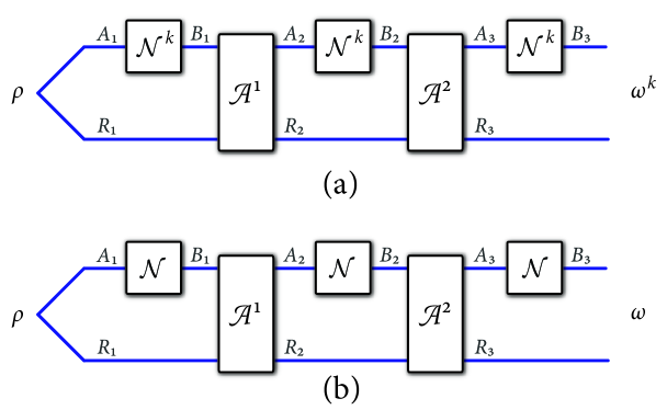
Figure 2: Adaptive protocol for distinguishing three uses of the channel $\mathcal{N}_{A\rightarrow B}^{k}$ from three uses of $\mathcal{N}_{A\rightarrow B}$. The protocol is denoted by $\mathcal{P}^{(3)}$ and consists of state preparation $\rho_{R_{1}A_{1}}$, as well as the channels $\mathcal{A}_{R_{1}B_{1}\rightarrow R_{2}A_{2}}^{(1)}$ and $\mathcal{A}_{R_{2}B_{2}\rightarrow R_{3}A_{3}}^{(2)}$. (a) The protocol $\mathcal{P}^{(3)}$ is used with three uses of the channel $\mathcal{N}_{A\rightarrow B}^{k}$, and the final state is $\omega_{R_{3}B_{3}}^{k}$. (b) The protocol $\mathcal{P}^{(3)}$ is used with three uses of the channel $\mathcal{N}_{A\rightarrow B}$, and the final state is $\omega_{R_{3}B_{3}}$. Strong convergence of the channel sequence $\{\mathcal{N}_{A\rightarrow B}^{k}\}_{k}$ to $\mathcal{N}_{A\rightarrow B}$ implies that, given a fixed protocol $\mathcal{P}^{(3)}$, the infidelity of the states $\omega_{R_{3}B_{3}}^{k}$ and $\omega_{R_{3}B_{3}}$ converges to zero in the limit as $k\rightarrow\infty$.

In this general context, strong convergence corresponds to the following statement: for a given protocol $\mathcal{P}^{(n)}$, the following limit holds

$$\lim_{k\rightarrow\infty}\varepsilon_{\text{ad}}^{(n)}(k,\mathcal{P}^{(n)})=0,$$ (48)

or more compactly,

$$\sup_{\mathcal{P}^{(n)}}\lim_{k\rightarrow\infty}\varepsilon_{\text{ad}}^{(n)}(k,\mathcal{P}^{(n)})=0.$$ (49)

Uniform convergence again corresponds to a swap of the supremum and limit

$$\lim_{k\rightarrow\infty}\sup_{\mathcal{P}^{(n)}}\varepsilon_{\text{ad}}^{(n)}(k,\mathcal{P}^{(n)})=0,$$ (50)

and again, it should typically be avoided in physical applications as it is too strong and not needed for most purposes, following the suggestions of (SH08, , Section 3).

I now explicitly show that strong convergence of the sequence $\{\mathcal{N}_{A\rightarrow B}^{k}\}_{k}$ implies strong convergence of $n$ uses of each channel in this sequence in this general sense. The proof is elementary and similar to that in (29)–(30), making use of the triangle inequality and data processing of fidelity. It bears similarities to numerous prior results in the literature BBBV97 ; BBHT98 ; Z99 ; BHLS03 ; CMW14 ; TGW14 ; TGW14Nat ; Christandl2017 , in which adaptive protocols were analyzed. For simplicity, we can focus on the case of $n=3$ and then the proof is easily extended. Begin by considering a fixed protocol $\mathcal{P}^{(3)}$. Then consider that

$$\sqrt{\varepsilon_{\text{ad}}^{(3)}(k,\mathcal{P}^{(3)})} =P\left[\omega_{R_{3}B_{3}}^{k},\omega_{R_{3}B_{3}}\right]$$

$$=P\left[\left(\mathcal{N}^{k}\circ\mathcal{A}^{(2)}\circ\mathcal{N}^{k}\circ\mathcal{A}^{(1)}\circ\mathcal{N}^{k}\right)(\rho_{R_{1}A_{1}}),\left(\mathcal{N}\circ\mathcal{A}^{(2)}\circ\mathcal{N}\circ\mathcal{A}^{(1)}\circ\mathcal{N}\right)(\rho_{R_{1}A_{1}})\right]$$

$$\leq P\left[\left(\mathcal{N}^{k}\circ\mathcal{A}^{(2)}\circ\mathcal{N}^{k}\circ\mathcal{A}^{(1)}\circ\mathcal{N}^{k}\right)(\rho_{R_{1}A_{1}}),\left(\mathcal{N}^{k}\circ\mathcal{A}^{(2)}\circ\mathcal{N}^{k}\circ\mathcal{A}^{(1)}\circ\mathcal{N}\right)(\rho_{R_{1}A_{1}})\right]$$

$$\qquad+P\left[\left(\mathcal{N}^{k}\circ\mathcal{A}^{(2)}\circ\mathcal{N}^{k}\circ\mathcal{A}^{(1)}\circ\mathcal{N}\right)(\rho_{R_{1}A_{1}}),\left(\mathcal{N}^{k}\circ\mathcal{A}^{(2)}\circ\mathcal{N}\circ\mathcal{A}^{(1)}\circ\mathcal{N}\right)(\rho_{R_{1}A_{1}})\right]$$

$$\qquad+P\left[\left(\mathcal{N}^{k}\circ\mathcal{A}^{(2)}\circ\mathcal{N}\circ\mathcal{A}^{(1)}\circ\mathcal{N}\right)(\rho_{R_{1}A_{1}}),\left(\mathcal{N}\circ\mathcal{A}^{(2)}\circ\mathcal{N}\circ\mathcal{A}^{(1)}\circ\mathcal{N}\right)(\rho_{R_{1}A_{1}})\right]$$

$$\leq P\left[\mathcal{N}^{k}(\rho_{R_{1}A_{1}}),\mathcal{N}(\rho_{R_{1}A_{1}})\right]$$

$$\qquad+P\left[\mathcal{N}^{k}\left[(\mathcal{A}^{(1)}\circ\mathcal{N})(\rho_{R_{1}A_{1}})\right],\mathcal{N}\left[(\mathcal{A}^{(1)}\circ\mathcal{N})(\rho_{R_{1}A_{1}})\right]\right]$$

$$\qquad+P\left[\mathcal{N}^{k}\left[(\mathcal{A}^{(2)}\circ\mathcal{N}\circ\mathcal{A}^{(1)}\circ\mathcal{N})(\rho_{R_{1}A_{1}})\right],\mathcal{N}\left[(\mathcal{A}^{(2)}\circ\mathcal{N}\circ\mathcal{A}^{(1)}\circ\mathcal{N})(\rho_{R_{1}A_{1}})\right]\right],$$ (51)

where I have omitted some system labels for simplicity. The first inequality follows from the triangle inequality and the second from data processing of the fidelity under the channels

$$\mathcal{N}^{k}\circ\mathcal{A}^{(2)}\circ\mathcal{N}^{k}\circ\mathcal{A}^{(1)},\text{ and}$$ (52)

$$\mathcal{N}^{k}\circ\mathcal{A}^{(2)}.$$ (53)

The inequality in (51) can be understood as saying that the overall distinguishability of the $n$ uses of $\mathcal{N}^{k}$ and $\mathcal{N}$, as captured by $P\left[\omega_{R_{3}B_{3}}^{k},\omega_{R_{3}B_{3}}\right]$, is limited by the sum of the distinguishabilities at every step in the discrimination protocol (this is similar to the observations made in BBBV97 ; BBHT98 ; Z99 ; BHLS03 ; CMW14 ; TGW14 ; TGW14Nat ; Christandl2017 ). Now employing the inequality in (51), the facts that

$$\rho_{R_{1}A_{1}},$$ (54)

$$(\mathcal{A}^{(1)}\circ\mathcal{N})(\rho_{R_{1}A_{1}}),\text{ and}$$ (55)

$$(\mathcal{A}^{(2)}\circ\mathcal{N}\circ\mathcal{A}^{(1)}\circ\mathcal{N})(\rho_{R_{1}A_{1}})$$ (56)

are fixed states independent of $k$, the strong convergence of $\{\mathcal{N}_{A\rightarrow B}^{k}\}_{k}$, and taking the limit $k\rightarrow\infty$ on both sides of the inequality in (51), we conclude that for any fixed protocol $\mathcal{P}^{(3)}$, the following limit holds

$$\lim_{k\rightarrow\infty}\varepsilon_{\text{ad}}^{(3)}(k,\mathcal{P}^{(3)})=0.$$ (57)

By the same reasoning with the triangle inequality and data processing, the argument extends to any finite positive integer $n$, so that for any fixed protocol $\mathcal{P}^{(n)}$, the following limit holds

$$\lim_{k\rightarrow\infty}\varepsilon_{\text{ad}}^{(n)}(k,\mathcal{P}^{(n)})=0.$$ (58)

We can summarize the above development more compactly as

$$\sup_{\rho_{RA}}\lim_{k\rightarrow\infty}\varepsilon(k,\rho_{RA})=0\\ \Longrightarrow\sup_{\mathcal{P}^{(n)}}\lim_{k\rightarrow\infty}\varepsilon_{\text{ad}}^{(n)}(k,\mathcal{P}^{(n)})=0.$$ (59)

That is, strong convergence of the channel sequence $\{\mathcal{N}_{A\rightarrow B}^{k}\}_{k}$ implies strong convergence of $n$ uses of each channel $\mathcal{N}_{A\rightarrow B}^{k}$ in this sequence in any context in which the $n$ uses of $\mathcal{N}_{A\rightarrow B}^{k}$ could be invoked.

I end this subsection by noting the following proposition, having to do with the strong convergence of serial compositions of channel sequences. In fact, the serial composition result in (59) for adaptive protocols could be proven by employing only the following proposition and iterating.

Proposition 2

Let $\{\mathcal{N}_{A\rightarrow B}^{k}\}_{k}$ be a channel sequence that converges strongly to a channel $\mathcal{N}_{A\rightarrow B}$, and let $\{\mathcal{M}_{B\rightarrow C}^{k}\}_{k}$ be a channel sequence that converges strongly to a channel $\mathcal{M}_{B\rightarrow C}$. Then the channel sequence $\{\mathcal{M}_{B\rightarrow C}^{k}\circ\mathcal{N}_{A\rightarrow B}^{k}\}_{k}$ converges strongly to $\mathcal{M}_{B\rightarrow C}\circ\mathcal{N}_{A\rightarrow B}$.

Proof. A proof is similar to what is given above, and I give it for completeness. Let $\rho_{RA}$ be an arbitrary state. Consider that

$$P((\mathcal{M}_{B\rightarrow C}^{k}\circ\mathcal{N}_{A\rightarrow B}^{k})(\rho_{RA}),(\mathcal{M}_{B\rightarrow C}\circ\mathcal{N}_{A\rightarrow B})(\rho_{RA}))$$

$$\leq P((\mathcal{M}_{B\rightarrow C}^{k}\circ\mathcal{N}_{A\rightarrow B}^{k})(\rho_{RA}),(\mathcal{M}_{B\rightarrow C}^{k}\circ\mathcal{N}_{A\rightarrow B})(\rho_{RA}))$$

$$+P((\mathcal{M}_{B\rightarrow C}^{k}\circ\mathcal{N}_{A\rightarrow B})(\rho_{RA}),(\mathcal{M}_{B\rightarrow C}\circ\mathcal{N}_{A\rightarrow B})(\rho_{RA}))$$

$$\leq P(\mathcal{N}_{A\rightarrow B}^{k}(\rho_{RA}),\mathcal{N}_{A\rightarrow B}(\rho_{RA}))$$

$$+P((\mathcal{M}_{B\rightarrow C}^{k}\circ\mathcal{N}_{A\rightarrow B})(\rho_{RA}),(\mathcal{M}_{B\rightarrow C}\circ\mathcal{N}_{A\rightarrow B})(\rho_{RA})).$$ (60)

The first inequality follows from the triangle inequality and the second from data processing. Using the strong convergence of $\{\mathcal{N}_{A\rightarrow B}^{k}\}_{k}$ and $\{\mathcal{M}_{B\rightarrow C}^{k}\}_{k}$, the fact that $\mathcal{N}_{A\rightarrow B}(\rho_{RA})$ is a fixed state independent of $k$, applying the inequality in (60), and taking the limit $k\rightarrow\infty$, we find that

$$\!\!\!\!\lim_{k\rightarrow\infty}P((\mathcal{M}_{B\rightarrow C}^{k}\circ\mathcal{N}_{A\rightarrow B}^{k})(\rho_{RA}),(\mathcal{M}_{B\rightarrow C}\circ\mathcal{N}_{A\rightarrow B})(\rho_{RA}))\\ =0.$$ (61)

Since the state $\rho_{RA}$ was arbitrary, the proof is complete.   

II.5 Strong convergence in the teleportation simulation of bosonic Gaussian channels

The teleportation simulation of a bosonic Gaussian channel is another important notion to discuss. As found in NFC09 , single-mode, phase-covariant bosonic channels, such as the thermal, amplifier, or additive-noise channels, can be simulated by employing the bosonic teleportation protocol from prl1998braunstein . More general classes of bosonic Gaussian channels can be simulated as well WPG07 . In this subsection, I exclusively discuss single-mode bosonic Gaussian channels and extend the results later to particular multi-mode bosonic Gaussian channels. Denoting the original channel by $\mathcal{G}$, an unideal teleportation simulation of it realizes the bosonic Gaussian channel $\mathcal{G}^{\bar{\sigma}}\equiv\mathcal{G}\circ\mathcal{T}^{\bar{\sigma}}$, where $\mathcal{T}^{\bar{\sigma}}$ is the additive-noise channel from (11). This unideal teleportation simulation is possible due to the displacement covariance of bosonic Gaussian channels. Again, it is needed to clarify the meaning of the convergence $\mathcal{G}=\lim_{\bar{\sigma}\rightarrow 0}\mathcal{G}^{\bar{\sigma}}$. Based on the previous discussions in this paper, it is clear that the convergence should be considered in the strong sense in most applications: for a state $\rho_{RA}$, we have that

$$\lim_{\bar{\sigma}\rightarrow 0}\left[1-F((\operatorname{id}_{R}\otimes\mathcal{G}_{A})(\rho_{RA}),(\operatorname{id}_{R}\otimes\mathcal{G}_{A}^{\bar{\sigma}})(\rho_{RA}))\right]=0,$$ (62)

where $F$ denotes the quantum fidelity. This equality follows as a consequence of (16) and the data-processing inequality for fidelity.

As a consequence of (36) and data processing, we also have the following convergence for a teleportation simulation of the tensor-power channel $\mathcal{G}^{\otimes n}$: for a state $\rho_{RA^{n}}$, we have that

$$\lim_{\bar{\sigma}\rightarrow 0}\left[1-F(\mathcal{G}_{A}^{\otimes n}(\rho_{RA^{n}}),(\mathcal{G}_{A}^{\bar{\sigma}})^{\otimes n}(\rho_{RA^{n}}))\right]=0,$$ (63)

where the identity map $\operatorname{id}_{R}$ is omitted for simplicity.

Finally, the argument from Section II.4 applies to the teleportation simulation of bosonic Gaussian channels as well. In more detail, the strong convergence of $\mathcal{G}^{\bar{\sigma}}$ to $\mathcal{G}$ in the limit $\bar{\sigma}\rightarrow 0$ implies strong convergence of $n$ uses of $\mathcal{G}^{\bar{\sigma}}$ to $n$ uses of $\mathcal{G}$ in the general sense discussed in Section II.4. That is, as a consequence of (17) and (59), we have that

$$\sup_{\mathcal{P}^{(n)}}\lim_{\bar{\sigma}\rightarrow 0}\varepsilon_{\text{ad}}^{(n)}(\bar{\sigma},\mathcal{P}^{(n)})=0,$$ (64)

where $\varepsilon_{\text{ad}}^{(n)}(\bar{\sigma},\mathcal{P}^{(n)})$ is defined by replacing $\mathcal{N}_{A\rightarrow B}^{k}$ with $\mathcal{G}^{\bar{\sigma}}$ and $\mathcal{N}_{A\rightarrow B}$ with $\mathcal{G}$ in (45), (46), and (47).

II.6 Uniform convergence in the teleportation simulations of pure-loss, thermal, pure-amplifier, amplifier, and additive-noise channels

I now prove that the teleportation simulations of pure-loss, thermal, pure-amplifier, amplifier, and additive-noise channels converge uniformly to the original channels, in the limit of ideal squeezing and detection for the simulations. The argument for uniform convergence is elementary, using the structure of these channels and their teleportation simulations, as well as a data processing argument that is the same as that which was employed in TW16 ; SWAT17 . Note that these uniform convergence results are in contrast to the teleportation simulation of the ideal channel, where the convergence occurs in the strong sense but not in the uniform sense.

To prove the uniform convergence of the teleportation simulations of the aforementioned channels, let us start with the thermal channel. Consider that the thermal channel $\mathcal{L}_{\eta,N_{B}}$ of transmissivity $\eta\in(0,1)$ and thermal photon number $N_{B}\geq 0$ is completely specified by its action on the $2\times 1$ mean vector $s$ and $2\times 2$ covariance matrix $V$ of a single-mode input S17 :

$$s \rightarrow Xs,$$ (65)

$$V \rightarrow XVX^{T}+Y,$$ (66)

where

$$X =\sqrt{\eta}I_{2},$$ (67)

$$Y =(1-\eta)(2N_{B}+1)I_{2},$$ (68)

and $I_{2}$ denotes the $2\times 2$ identity matrix. An unideal teleportation simulation of a thermal channel is equivalent to the serial concatenation of the additive-noise channel $\mathcal{T}^{\bar{\sigma}}$ with variance $\bar{\sigma}>0$, followed by the thermal channel $\mathcal{L}_{\eta,N_{B}}$, as discussed in Section II.5. Since the additive-noise channel has the same action as in (65) and (66), but with

$$X =I_{2},$$ (69)

$$Y =2\bar{\sigma}I_{2},$$ (70)

we find, after composing and simplifying, that the simulating channel $\mathcal{L}_{\eta,N_{B}}\circ\mathcal{T}^{\bar{\sigma}}$ has the same action as in (65) and (66), but with

$$X =\sqrt{\eta}I_{2},$$ (71)

$$Y =\left[\eta 2\bar{\sigma}+(1-\eta)(2N_{B}+1)\right]I_{2}$$ (72)

$$=(1-\eta)(2\left[N_{B}+\eta\bar{\sigma}/(1-\eta)\right]+1)I_{2}.$$ (73)

This latter finding means that the simulating channel $\mathcal{L}_{\eta,N_{B}}\circ\mathcal{T}^{\bar{\sigma}}$ is equivalent to the thermal channel $\mathcal{L}_{\eta,N_{B}+\eta\bar{\sigma}/(1-\eta)}$, i.e.,

$$\mathcal{L}_{\eta,N_{B}}\circ\mathcal{T}^{\bar{\sigma}}=\mathcal{L}_{\eta,N_{B}+\eta\bar{\sigma}/(1-\eta)}.$$ (74)

Let us set

$$N_{B}^{\prime}\equiv N_{B}+\eta\bar{\sigma}/(1-\eta).$$ (75)

Note that any thermal channel $\mathcal{L}_{\eta,N_{B}}$ can be realized in three steps:

1. prepare an environment mode in a thermal state $\theta(N_{B})$ of mean photon number $N_{B}\geq 0$, where

   $$\theta(N_{B})=\frac{1}{N_{B}+1}\sum_{n=0}^{\infty}\left(\frac{N_{B}}{N_{B}+1}\right)^{n}|n\rangle\langle n|,$$ (76)

2. interact the channel input mode with the environment mode at a unitary beamsplitter $\mathcal{B}_{\eta}$ of transmissivity $\eta$, and

3. discard the environment mode.

This observation and that in (74) are what lead to uniform convergence of the simulating channel $\mathcal{L}_{\eta,N_{B}^{\prime}}$ to the original channel $\mathcal{L}_{\eta,N_{B}}$ in the limit as $\bar{\sigma}\rightarrow 0$. Indeed, let $\rho_{RA}$ be an arbitrary input state, with $R$ a reference system corresponding to an arbitrary separable Hilbert space and system $A$ the channel input. Then we find that

$$P((\operatorname{id}_{R}\otimes\mathcal{L}_{\eta,N_{B}})(\rho_{RA}),(\operatorname{id}_{R}\otimes\mathcal{L}_{\eta,N_{B}^{\prime}})(\rho_{RA}))$$

$$\leq P((\operatorname{id}_{R}\otimes\mathcal{B}_{\eta})[\rho_{RA}\otimes\theta(N_{B})],(\operatorname{id}_{R}\otimes\mathcal{B}_{\eta})[\rho_{RA}\otimes\theta(N_{B}^{\prime})])$$

$$=P(\rho_{RA}\otimes\theta(N_{B}),\rho_{RA}\otimes\theta(N_{B}^{\prime}))$$

$$=P(\theta(N_{B}),\theta(N_{B}^{\prime}))$$

$$\equiv e(N_{B},\eta,\bar{\sigma}),$$ (77)

where $e(N_{B},\eta,\bar{\sigma})$ explicitly evaluates to

$$e(N_{B},\eta,\bar{\sigma})=\\ \Bigg{[}1-\Big{[}\sqrt{\left(N_{B}+1\right)\left(N_{B}+\eta\bar{\sigma}/(1-\eta)+1\right)}\\ -\sqrt{N_{B}\left[N_{B}+\eta\bar{\sigma}/(1-\eta)\right]}\Big{]}^{-2}\Bigg{]}^{1/2}.$$ (78)

The explicit evaluation in (78) is a direct consequence of (TW16, , Eqs. (34)–(35)), found by evaluating the fidelity between two thermal states of respective mean photon numbers $N_{B}$ and $N_{B}+\eta\bar{\sigma}/(1-\eta)$. See also H75 ; S98 for formulas for the fidelity of single-mode Gaussian states. The first inequality in (77) follows from data processing. The first equality follows from unitary invariance of the metric $P$ and the second from its invariance under tensoring in the same state $\rho_{RA}$. To summarize the inequality in (77), it is stating that the distinguishability of the channels $\mathcal{L}_{\eta,N_{B}}$ and $\mathcal{L}_{\eta,N_{B}^{\prime}}$, when allowing for any input probe state $\rho_{RA}$, is limited by the distinguishability of the environment states $\theta(N_{B})$ and $\theta(N_{B}^{\prime})$, and this is similar to the observations made in TW16 ; SWAT17 . Thus, the bound in (77) is a uniform bound, holding for all input states $\rho_{RA}$, and so we conclude that

$$\sup_{\rho_{RA}}P((\operatorname{id}_{R}\otimes\mathcal{L}_{\eta,N_{B}})(\rho_{RA}),(\operatorname{id}_{R}\otimes\mathcal{L}_{\eta,N_{B}^{\prime}})(\rho_{RA}))\\ \leq e(N_{B},\eta,\bar{\sigma}).$$ (79)

Now taking the limit $\bar{\sigma}\rightarrow 0$ and using the fact that $\lim_{\bar{\sigma}\rightarrow 0}e(N_{B},\eta,\bar{\sigma})=0$ for $\eta\in(0,1)$ and $N_{B}\geq 0$, we find that

$$\lim_{\bar{\sigma}\rightarrow 0}\sup_{\rho_{RA}}P((\operatorname{id}_{R}\otimes\mathcal{L}_{\eta,N_{B}})(\rho_{RA}),(\operatorname{id}_{R}\otimes\mathcal{L}_{\eta,N_{B}^{\prime}})(\rho_{RA}))=0.$$ (80)

Thus, the teleportation simulation $\mathcal{L}_{\eta,N_{B}}\circ\mathcal{T}^{\bar{\sigma}}$ of the thermal channel $\mathcal{L}_{\eta,N_{B}}$ of transmissivity $\eta\in(0,1)$ and thermal photon number $N_{B}\geq 0$ converges uniformly to the thermal channel.

The above uniform convergence result holds in particular for a pure-loss channel of transmissivity $\eta\in(0,1)$, because this channel is a thermal channel with $N_{B}=0$. That is, the environment state for the pure-loss channel is a vacuum state, and its teleportation simulation is a thermal channel with the same transmissivity and environment state given by a thermal state of mean photon number $\eta\bar{\sigma}/(1-\eta)$. In this case, the uniform upper bound $e(N_{B}=0,\eta,\bar{\sigma})$ simplifies to

$$e(N_{B}=0,\eta,\bar{\sigma})=\sqrt{1-\frac{1}{\eta\bar{\sigma}/(1-\eta)+1}},$$ (81)

for which we clearly have that $\lim_{\bar{\sigma}\rightarrow 0}e(N_{B}=0,\eta,\bar{\sigma})=0$. Thus, the teleportation simulation of a pure-loss channel $\mathcal{L}_{\eta,N_{B}=0}$ converges uniformly to $\mathcal{L}_{\eta,N_{B}=0}$.

Similar results hold for the pure-amplifier and amplifier channels. Indeed, to see this, let us begin by considering a general amplifier channel $\mathcal{A}_{G,N_{B}}$ of gain $G>1$ and thermal photon number $N_{B}\geq 0$. Such a channel has the action as in (65) and (66), but with

$$X =\sqrt{G}I_{2},$$ (82)

$$Y =(G-1)(2N_{B}+1)I_{2}.$$ (83)

By similar reasoning as before, the teleportation simulation $\mathcal{A}_{G,N_{B}}\circ\mathcal{T}^{\bar{\sigma}}$ of the amplifier channel has the action as in (65) and (66), but with

$$X =\sqrt{G}I_{2},$$ (84)

$$Y =\left[G2\bar{\sigma}+(G-1)(2N_{B}+1)\right]I_{2}$$ (85)

$$=(G-1)(2\left[N_{B}+G\bar{\sigma}/(G-1)\right]+1)I_{2}.$$ (86)

Thus, the teleportation simulation $\mathcal{A}_{G,N_{B}}\circ\mathcal{T}^{\bar{\sigma}}$ is equivalent to an amplifier channel $\mathcal{A}_{G,N_{B}+G\bar{\sigma}/(G-1)}$:

$$\mathcal{A}_{G,N_{B}}\circ\mathcal{T}^{\bar{\sigma}}=\mathcal{A}_{G,N_{B}+G\bar{\sigma}/(G-1)}.$$ (87)

An amplifier channel $\mathcal{A}_{G,N_{B}}$ can be realized by the following three steps:

1. prepare an environment mode in a thermal state $\theta(N_{B})$ of mean photon number $N_{B}\geq 0$,

2. interact the channel input mode with the environment mode using a unitary two-mode squeezer $\mathcal{S}_{G}$ of gain $G$, and

3. discard the environment mode.

For an arbitrary state $\rho_{RA}$, we find the following upper bound by the same reasoning as in (77), but replacing the beamsplitter $\mathcal{B}_{\eta}$ therein by the two-mode squeezer $\mathcal{S}_{G}$,

$$P((\operatorname{id}_{R}\otimes\mathcal{A}_{G,N_{B}})(\rho_{RA}),(\operatorname{id}_{R}\otimes\mathcal{A}_{G,N_{B}^{\prime\prime}})(\rho_{RA}))\\ \leq P(\theta(N_{B}),\theta(N_{B}^{\prime\prime}))\equiv e(N_{B},G,\bar{\sigma})$$ (88)

where

$$N_{B}^{\prime\prime}\equiv N_{B}+G\bar{\sigma}/(G-1)$$ (89)

and

$$e(N_{B},G,\bar{\sigma})=\\ \Bigg{[}1-\Big{[}\sqrt{\left(N_{B}+1\right)\left(N_{B}+G\bar{\sigma}/(G-1)+1\right)}\\ -\sqrt{N_{B}\left[N_{B}+G\bar{\sigma}/(G-1)\right]}\Big{]}^{-2}\Bigg{]}^{1/2}.$$ (90)

Again, the inequality in (88) is the statement that the distinguishability of the channels $\mathcal{A}_{G,N_{B}}$ and $\mathcal{A}_{G,N_{B}^{\prime\prime}}$, when allowing for any input probe state $\rho_{RA}$, is limited by the distinguishability of the channel environment states $\theta(N_{B})$ and $\theta(N_{B}^{\prime\prime})$. Given that the bound in (88) is a uniform bound holding for all input states $\rho_{RA}$, this implies that

$$\sup_{\rho_{RA}}P((\operatorname{id}_{R}\otimes\mathcal{A}_{G,N_{B}})(\rho_{RA}),(\operatorname{id}_{R}\otimes\mathcal{A}_{G,N_{B}^{\prime\prime}})(\rho_{RA}))\\ \leq e(N_{B},G,\bar{\sigma})$$ (91)

We can then take the limit $\bar{\sigma}\rightarrow 0$ and use the fact that $\lim_{\bar{\sigma}\rightarrow 0}e(N_{B},G,\bar{\sigma})=0$ for all $G>1$ and $N_{B}\geq 0$ to find that

$$\lim_{\bar{\sigma}\rightarrow 0}\sup_{\rho_{RA}}P((\operatorname{id}_{R}\otimes\mathcal{A}_{G,N_{B}})(\rho_{RA}),(\operatorname{id}_{R}\otimes\mathcal{A}_{G,N_{B}^{\prime\prime}})(\rho_{RA}))=0.$$ (92)

Thus, the teleportation simulation $\mathcal{A}_{G,N_{B}}\circ\mathcal{T}^{\bar{\sigma}}$ of the amplifier channel $\mathcal{A}_{G,N_{B}}$ converges uniformly to it, for all $G>1$ and thermal photon number $N_{B}\geq 0$.

The pure-amplifier channel is a special case of the amplifier channel $\mathcal{A}_{G,N_{B}}$ with $N_{B}=0$, so that the above analysis applies and the teleportation simulation of the pure-amplifier channel $\mathcal{A}_{G,N_{B}=0}$ converges uniformly to it. Indeed, the uniform upper bound $e(N_{B}=0,G,\bar{\sigma})$ simplifies as

$$P((\operatorname{id}_{R}\otimes\mathcal{A}_{G,N_{B}=0})(\rho_{RA}),(\operatorname{id}_{R}\otimes\mathcal{A}_{G,G\bar{\sigma}/(G-1)})(\rho_{RA}))\\ \leq e(N_{B}=0,G,\bar{\sigma})=\sqrt{1-\frac{1}{G\bar{\sigma}/(G-1)+1}},$$ (93)

and so it is clear that

$$\lim_{\bar{\sigma}\rightarrow 0}\sup_{\rho_{RA}}P(\mathcal{A}_{G,0}(\rho_{RA}),\mathcal{A}_{G,G\bar{\sigma}/(G-1)}(\rho_{RA}))=0,$$ (94)

where I have omitted the identity maps $\operatorname{id}_{R}$ acting on system $R$ for simplicity.

A similar argument establishes that the teleportation simulation of the additive-noise channel $\mathcal{T}^{\xi}$ with variance $\xi>0$ converges uniformly to it. To see this, let us begin by noting that any additive-noise channel $\mathcal{T}^{\xi}$ can be realized by the following three steps:

1. Prepare a continuous classical environment register according to the complex Gaussian distribution $G_{\xi}(\alpha)$, as defined in (12).

2. Based on the classical value $\alpha$ in the environment register, apply a unitary displacement operation $D(\alpha)$ to the channel input. This step can be described as an interaction channel $\mathcal{C}$ between the channel input and the environment register.

3. Finally, discard the environment register.

Also, note that the fidelity between two complex Gaussian distributions of variances $\xi_{1},\xi_{2}>0$ is given by

$$F(G_{\xi_{1}},G_{\xi_{2}})=\frac{4\xi_{1}\xi_{2}}{\left(\xi_{1}+\xi_{2}\right)^{2}},$$ (95)

which one may verify directly or consult CA79 . Then, proceeding as in the previous proofs, we have for an arbitrary input state $\rho_{RA}$ that

$$P((\operatorname{id}_{R}\otimes\mathcal{T}^{\xi})(\rho_{RA}),(\operatorname{id}_{R}\otimes\mathcal{T}^{\xi+\bar{\sigma}})(\rho_{RA}))$$

$$\leq P((\operatorname{id}_{R}\otimes\mathcal{C})(\rho_{RA}\otimes G_{\xi}),(\operatorname{id}_{R}\otimes\mathcal{C})(\rho_{RA}\otimes G_{\xi+\bar{\sigma}}))$$

$$\leq P(\rho_{RA}\otimes G_{\xi},\rho_{RA}\otimes G_{\xi+\bar{\sigma}})$$

$$=P(G_{\xi},G_{\xi+\bar{\sigma}})$$

$$=\sqrt{1-\frac{4\xi(\xi+\bar{\sigma})}{(2\xi+\bar{\sigma})^{2}}}.$$ (96)

The first and second inequalities follow from data processing. The first equality follows because the metric $P$ is invariant under tensoring in the same state $\rho_{RA}$. The final equality follows from the definition of the metric $P$ and the formula in (95). As in the other proofs, the inequality in (96) is intuitive, indicating that the distinguishability of the channels $\mathcal{T}^{\xi}$ and $\mathcal{T}^{\xi+\bar{\sigma}}$ is limited by the distinguishability of the underlying classical distributions $G_{\xi}$ and $G_{\xi+\bar{\sigma}}$. The bound in (96) is a uniform bound, holding for all input states $\rho_{RA}$, and so we conclude that

$$\sup_{\rho_{RA}}P((\operatorname{id}_{R}\otimes\mathcal{T}^{\xi})(\rho_{RA}),(\operatorname{id}_{R}\otimes\mathcal{T}^{\xi+\bar{\sigma}})(\rho_{RA}))\\ \leq\sqrt{1-\frac{4\xi(\xi+\bar{\sigma})}{(2\xi+\bar{\sigma})^{2}}}.$$ (97)

Finally, we take the limit as $\bar{\sigma}\rightarrow 0$ to establish the uniform convergence of the teleportation simulation of the additive-noise channel of variance $\xi>0$ to itself:

$$\lim_{\bar{\sigma}\rightarrow 0}\sup_{\rho_{RA}}P((\operatorname{id}_{R}\otimes\mathcal{T}^{\xi})(\rho_{RA}),(\operatorname{id}_{R}\otimes\mathcal{T}^{\xi+\bar{\sigma}})(\rho_{RA}))=0.$$ (98)

Remark 3

By the results of TW16 , the uniform upper bounds in (79), (91), and (97) are all achievable and are thus equalities. The achievable strategy consists of taking the input states $\rho_{RA}$ to be a sequence of two-mode squeezed vacuum states with photon number $N_{S}$ tending to infinity.

Remark 4

On the one hand, the thermal, amplifier, and additive-noise channels are the single-mode bosonic Gaussian channels that are of major interest in applications, as stressed in (HG12, , Section 3.5) and (H12, , Section 12.6.3). On the other hand, one could consider generalizing the results of this section to arbitrary single-mode bosonic Gaussian channels. In doing so, one should consider the Holevo classification of single-mode bosonic Gaussian channels Holevo2007 . However, there is little reason to generalize the contents of this section to other channels in the Holevo classification. The thermal and amplifier channels form the class $C$ discussed in Holevo2007 , and the additive-noise channels form the class $B_{2}$ from Holevo2007 , which I have already considered in this section. The classes that remain are labeled $A$, $B_{1}$, and $D$. The channels in classes $A$ and $D$ are entanglement breaking, as proved in Holevo2008 . Thus, the channels in classes $A$ and $D$ can be directly realized by the action of an LOCC on the input state (without any need for an entangled resource state), and thus we would never have any reason to be interested in the teleportation simulation of these channels. The final remaining class is $B_{1}$, but channels in the class $B_{1}$ do not seem to be interesting in physical applications.

Remark 5

The class $B_{1}$ has been considered in P18 , where it was shown that the teleportation simulation of a channel in this class does not converge uniformly, similar to what occurs for the identity channel. Based on the above, and the fact that the ideal channel and channels in the class $B_{1}$ have unconstrained quantum capacity equal to infinity Holevo2007 , as well as the fact that channels in the classes $C$ and $B_{2}$ have finite unconstrained quantum capacity SWAT17 , we can conclude that, among the single-mode bosonic Gaussian channels that are not entanglement breaking, their teleportation simulations converge uniformly if and only if their unconstrained quantum capacity is finite. This establishes a non-trivial link between teleportation simulation and unconstrained quantum capacity.

II.7 Generalization of uniform convergence results to multi-mode bosonic Gaussian channels

In this section, I discuss a generalization of the results of the previous section to the case of multi-mode bosonic Gaussian channels . Before doing so, I give a brief review of bosonic Gaussian states and channels (see CEGH08 for a more comprehensive review). Let

$$\hat{R}\equiv\left[\hat{q}_{1},\ldots,\hat{q}_{m},\hat{p}_{1},\ldots,\hat{p}_{m}\right]\equiv\left[\hat{x}_{1},\ldots,\hat{x}_{2m}\right]$$ (99)

denote a row vector of position- and momentum-quadrature operators, satisfying the canonical commutation relations:

$$\left[\hat{R}_{j},\hat{R}_{k}\right]=i\Omega_{j,k},\quad\text{where}\quad\Omega\equiv\begin{bmatrix}0&1\\ -1&0\end{bmatrix}\otimes I_{m},$$ (100)

and $I_{m}$ denotes the $m\times m$ identity matrix. We take the annihilation operator for the $j$th mode as $\hat{a}_{j}=(\hat{q}_{j}+i\hat{p}_{j})/\sqrt{2}$. For $z$ a column vector in $\mathbb{R}^{2m}$, we define the unitary displacement operator $D(z)=D^{\dagger}(-z)\equiv\exp(i\hat{R}z)$. Displacement operators satisfy the following relation:

$$D(z)D(z^{\prime})=D(z+z^{\prime})\exp\!\left(-\frac{i}{2}z^{T}\Omega z^{\prime}\right).$$ (101)

Every state $\rho\in\mathcal{D}(\mathcal{H})$ has a corresponding Wigner characteristic function, defined as

$$\chi_{\rho}(z)\equiv\operatorname{Tr}\{D(z)\rho\},$$ (102)

and from which we can obtain the state $\rho$ as

$$\rho=\int\frac{d^{2m}z}{\left(2\pi\right)^{m}}\ \chi_{\rho}(z)\ D^{{\dagger}}(z).$$ (103)

A quantum state $\rho$ is Gaussian if its Wigner characteristic function has a Gaussian form as

$$\chi_{\rho}(\xi)=\exp\left(-\frac{1}{4}z^{T}V^{\rho}z+i\left[\mu^{\rho}\right]^{T}z\right),$$ (104)

where $\mu^{\rho}$ is the $2m\times 1$ mean vector of $\rho$, whose entries are defined by $\mu_{j}^{\rho}\equiv\langle\hat{R}_{j}\rangle_{\rho}$ and $V^{\rho}$ is the $2m\times 2m$ covariance matrix of $\rho$, whose entries are defined as

$$V_{j,k}^{\rho}\equiv\langle\{\hat{R}_{j}-\mu_{j}^{\rho},\hat{R}_{k}-\mu_{k}^{\rho}\}\rangle_{\rho}.$$ (105)

The following condition holds for a valid covariance matrix: $V\geq i\Omega$, which is a manifestation of the uncertainty principle.

A $2m\times 2m$ matrix $S$ is symplectic if it preserves the symplectic form: $S\Omega S^{T}=\Omega$. According to Williamson’s theorem W36 , there is a diagonalization of the covariance matrix $V^{\rho}$ of the form,

$$V^{\rho}=S^{\rho}\left(D^{\rho}\oplus D^{\rho}\right)\left(S^{\rho}\right)^{T},$$ (106)

where $S^{\rho}$ is a symplectic matrix and $D^{\rho}\equiv\operatorname{diag}(\nu_{1},\ldots,\nu_{m})$ is a diagonal matrix of symplectic eigenvalues such that $\nu_{i}\geq 1$ for all $i\in\left\{1,\ldots,m\right\}$. Computing this decomposition is equivalent to diagonalizing the matrix $iV^{\rho}\Omega$ (WTLB16, , Appendix A).

The Hilbert–Schmidt adjoint of a Gaussian quantum channel $\mathcal{N}_{X,Y}$ from $m$ modes to $m$ modes has the following effect on a displacement operator $D(z)$ CEGH08 :

$$D(z)\longmapsto D(Xz)\exp\left(-\frac{1}{4}z^{T}Yz+iz^{T}d\right),$$ (107)

where $X$ is a real $2m\times 2m$ matrix, $Y$ is a real $2m\times 2m$ positive semi-definite matrix, and $d\in\mathbb{R}^{2m}$, such that they satisfy

$$Y\geq i\left[\Omega-X^{T}\Omega X\right].$$ (108)

The effect of the channel on the mean vector $\mu^{\rho}$ and the covariance matrix $V^{\rho}$ is thus as follows:

$$\mu^{\rho} \longmapsto X^{T}\mu^{\rho}+d,$$ (109)

$$V^{\rho} \longmapsto X^{T}V^{\rho}X+Y.$$ (110)

All Gaussian channels are covariant with respect to displacement operators, and this is the main reason why they are teleportation simulable, as noted in WPG07 ; NFC09 . That is, the following relation holds

$$\mathcal{N}_{X,Y}(D(z)\rho D^{{\dagger}}(z))=D(X^{T}z)\mathcal{N}_{X,Y}(\rho)D^{{\dagger}}(X^{T}z).$$ (111)

Just as every quantum channel can be implemented as a unitary transformation on a larger space followed by a partial trace S55 , so can Gaussian channels be implemented as a Gaussian unitary on a larger space with some extra modes prepared in the vacuum state, followed by a partial trace CEGH08 . Given a Gaussian channel $\mathcal{N}_{X,Y}$ with $Z$ such that $Y=ZZ^{T}$ we can find two other matrices $X_{E}$ and $Z_{E}$ such that there is a symplectic matrix

$$S=\begin{bmatrix}X^{T}&Z\\ X_{E}^{T}&Z_{E}\end{bmatrix},$$ (112)

which corresponds to the Gaussian unitary transformation on a larger space.

Alternatively, for certain Gaussian channels, there is a realization that is analogous to those discussed in the previous section for the thermal, amplifier, and additive-noise channels. In particular, consider a Gaussian channel with $X$ and $Y$ matrices as discussed above, and suppose that the mean vector $d=0$ (note that the condition $d=0$ is not particularly restrictive because it just corresponds to a unitary displacement at the input or output of the channel, and capacities or distinguishability measures do not change under such unitary actions). Whenever the matrix $\Omega-X^{T}\Omega X$ is full rank, implying then by (108) that $Y$ is full rank, the Gaussian channel can be realized as follows (CEGH08, , Theorem 1):

$$\rho_{A}\rightarrow\mathcal{N}_{X,Y}(\rho_{A})=\operatorname{Tr}_{E}\{U_{AE}(\rho_{A}\otimes\gamma_{E}(Y))U_{AE}^{{\dagger}}\},$$ (113)

where $\rho_{A}$ is the $m$-mode input, $\gamma_{E}(Y)$ is a zero-mean, $m$-mode Gaussian state with covariance matrix given by $KYK^{T}$, where $K$ is the invertible matrix discussed around (CEGH08, , Eqs. (27)–(28)), and $U_{AE}$ is a Gaussian unitary acting on $2m$ modes.

Given the above result, we can then generalize the argument from the previous section to argue that the teleportation simulations of these channels converge uniformly. Indeed, as discussed in WPG07 and as a generalization of the single-mode case discussed previously, the teleportation simulation of a Gaussian channel $\mathcal{N}_{X,Y}$ realizes the Gaussian channel $\mathcal{N}_{X,Y+\bar{\sigma}I}$, where $\bar{\sigma}>0$ is a parameter characterizing the squeezing strength and the unideal detections involved in the teleportation simulation. Thus, as before, the teleportation simulation of a Gaussian channel simply acts as an additive-noise channel concatenated with the original channel, and the effect is that the noise matrix for the channel realized from the teleportation simulation is $Y+\bar{\sigma}I$, while the $X$ matrix is unaffected. Thus, invoking (CEGH08, , Theorem 1), the teleportation simulation $\mathcal{N}_{X,Y+\bar{\sigma}I}$ can be realized as the following transformation:

$$\rho_{A}\rightarrow\mathcal{N}_{X,Y}(\rho_{A})=\operatorname{Tr}_{E}\{U_{AE}(\rho_{A}\otimes\gamma_{E}(Y+\bar{\sigma}I))U_{AE}^{{\dagger}}\}.$$ (114)

Then we are led to the following theorem:

Theorem 6

Let $\mathcal{N}_{X,Y}$ be a multi-mode quantum Gaussian channel of the form in (107)–(110), such that $\Omega-X^{T}\Omega X$ is full rank. Then its teleportation simulation converges uniformly, in the sense that

$$\sup_{\rho_{RA}}P[(\operatorname{id}_{R}\otimes\mathcal{N}_{X,Y})(\rho_{RA}),(\operatorname{id}_{R}\otimes\mathcal{N}_{X,Y+\bar{\sigma}I})(\rho_{RA})]\\ \leq P(\gamma_{E}(Y),\gamma_{E}(Y+\bar{\sigma}I)),$$ (115)

where $\gamma_{E}(Y)$ is defined in (113),

$$\lim_{\bar{\sigma}\rightarrow 0}P(\gamma_{E}(Y),\gamma_{E}(Y+\bar{\sigma}I))=0,$$ (116)

and one can use the explicit formula (PS00, , Section IV) for the fidelity of multi-mode, zero-mean Gaussian states to find an analytical expression for

$$P(\gamma_{E}(Y),\gamma_{E}(Y+\bar{\sigma}I))=\sqrt{1-F(\gamma_{E}(Y),\gamma_{E}(Y+\bar{\sigma}I))},$$ (117)

for $\bar{\sigma}>0$.

Proof. The proof of this theorem follows the same strategy given in the previous section, which in turn was used in TW16 ; SWAT17 . In detail, letting $\rho_{RA}$ be an arbitrary state, we have that

$$P[(\operatorname{id}_{R}\otimes\mathcal{N}_{X,Y})(\rho_{RA}),(\operatorname{id}_{R}\otimes\mathcal{N}_{X,Y+\bar{\sigma}I})(\rho_{RA})]$$

$$\leq P[U_{AE}(\rho_{RA}\otimes\gamma_{E}(Y))U_{AE}^{{\dagger}},U_{AE}(\rho_{RA}\otimes\gamma_{E}(Y^{\bar{\sigma}}))U_{AE}^{{\dagger}}]$$

$$=P[\rho_{RA}\otimes\gamma_{E}(Y),\rho_{RA}\otimes\gamma_{E}(Y+\bar{\sigma}I)]$$

$$=P[\gamma_{E}(Y),\gamma_{E}(Y+\bar{\sigma}I)],$$ (118)

where $Y^{\bar{\sigma}}\equiv Y+\bar{\sigma}I$. The justification of these steps are the same as before, namely, data processing and unitary invariance. The above bound is clearly a uniform bound, holding for all states $\rho_{RA}$, and so we conclude (115).   

III Physical Interpretation with the CV Teleportation Game

We can interpret the results in the previous sections of this paper in a game-theoretic way, in order to further elucidate the physical meaning of the two kinds of convergence that we have considered in this paper. Let us consider a competitive game (call it the CV Teleportation Game) between a Distinguisher and a Teleporter, while an independent Referee determines who wins the game. At the outset, the Referee flips an unbiased coin and tells the outcome to the Teleporter. If the coin outcome is heads, then the Teleporter will apply the ideal channel. If it is tails, then he will apply the CV teleportation protocol. The game is such that either the Distinguisher reveals his strategy to the Teleporter beforehand, or vice versa. Furthermore, the Referee always learns the strategies of both the Distinguisher and the Teleporter. Everyone involved plays honestly. A particular instance of the game is depicted in Figure 3.

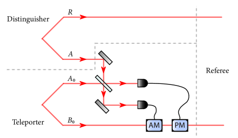
Figure 3: Depiction of the CV Teleportation Game, in the case that the coin outcome is tails, so that the Teleporter applies the continuous-variable bosonic teleportation protocol to the mode $A$ that the Distinguisher sends.

I now outline the full game in the case that the Distinguisher reveals his strategy to the Teleporter. In this case, the Distinguisher picks a pure state $\psi_{RA}$ and sends mode $A$ to the Teleporter and mode $R$ to the Referee. The Distinguisher also reveals a classical description of the state $\psi_{RA}$ to the Referee, and also to the Teleporter in this case. Based on this, the Teleporter can compute the entanglement infidelity $\varepsilon(\bar{\sigma},\psi_{RA})$ from (13) and can adjust the teleportation imperfection $\bar{\sigma}>0$ of his setup accordingly such that $\varepsilon(\bar{\sigma},\psi_{RA})\approx 0$. The Referee then reports the coin flip outcome to the Teleporter. If heads, then the Teleporter does nothing to mode $A$ (ideal channel); if tails, the Teleporter applies the continuous-variable bosonic teleportation protocol to mode $A$. The Teleporter sends the output mode to the Referee. The Referee then performs the optimal binary measurement H69 ; H73hel ; Hel76 to distinguish the two possible resulting states. If the measurement outcome is “heads,” then the channel applied by the Teleporter is decided to be the ideal channel. If the measurement outcome is “tails,” then the channel applied by the Teleporter is decided to be the teleportation channel. This procedure is then repeated a large number of times. If the fraction of rounds in which the coin flips match exceeds $3/4$, then the Distinguisher wins. Otherwise, the Teleporter wins.

To analyze the above physical setup, consider that the probability of distinguishing the channels in any single round is given by H69 ; H73hel ; Hel76

$$\Pr\{X=Y\}=\frac{1}{2}\left(1+\frac{1}{2}\left\|\psi_{RA}-\mathcal{T}_{A}^{\bar{\sigma}}(\psi_{RA})\right\|_{1}\right),$$ (119)

where $X$ is a Bernoulli random variable modeling the coin flip and $Y$ is a Bernoulli random variable modeling the measurement outcome. In the above described case in which the Distinguisher reveals his strategy, this means that the Teleporter can follow and choose $\bar{\sigma}$ as small as needed to guarantee that $\Pr\{X=Y\}<3/4$. Thus, with this structure to the game, the Teleporter wins with high probability after a large number of repetitions. In fact, based on well known relations between trace distance and fidelity Kholevo1972 ; FG98 , and the result given in (17), we have that

$$\sup_{\psi_{RA}}\inf_{\bar{\sigma}>0}\left\|\psi_{RA}-\mathcal{T}_{A}^{\bar{\sigma}}(\psi_{RA})\right\|_{1}=0.$$ (120)

Now suppose that the opposite scenario occurs in which the Teleporter reveals his strategy (and commits to it). This means that the teleportation imperfection $\bar{\sigma}>0$ is fixed at the outset. Then the Distinguisher can choose his input state to be the two-mode squeezed vacuum state $\Phi(N_{S})_{RA}$ such that $\varepsilon(\bar{\sigma},\Phi(N_{S})_{RA})\approx 1$, as considered in (21). This in turn means that the Distinguisher can guarantee that $\Pr\{X=Y\}>3/4$. Thus, in this case, the Distinguisher wins with high probability after a large number of repetitions. In fact, in this latter case, as a consequence of (21), we have that

$$\inf_{\bar{\sigma}>0}\sup_{\psi_{RA}}\left\|\psi_{RA}-\mathcal{T}_{A}^{\bar{\sigma}}(\psi_{RA})\right\|_{1}=2.$$ (121)

One may criticize whether the above game is truly physical. Indeed, it is never possible in practice to apply the ideal channel. Depending on the physical situation, the actual channel might be a pure-loss, thermal, pure-amplifier, amplifier or additive-noise channel, for example (one could further criticize “pure-loss” or “pure-amplifier”, but let us leave that). Let $\mathcal{G}_{A}$ denote one of these single-mode, phase-insensitive bosonic Gaussian channels. Suppose instead that the game changes in the following way: If the coin outcome is heads, then the Teleporter will apply the channel $\mathcal{G}$. If it is tails, then he will apply the teleportation simulation $\mathcal{G}_{A}\mathcal{\circ T}_{A}^{\bar{\sigma}}$ of $\mathcal{G}_{A}$.

There is a striking, physically observable difference in this case. No matter whether the Distinguisher reveals his strategy to the Teleporter, or the other way around, the Teleporter always wins with high probability! This is a direct consequence of the inequalities in (79), (91), and (97). Indeed, independent of the revealing, the Teleporter can simply compute the teleportation imperfection $\bar{\sigma}>0$, while incorporating his knowledge of the channel parameters, in order to always guarantee that $\Pr\{X=Y\}<3/4$. Thus, as a consequence of the mathematical fact that the teleportation simulations of these Gaussian channels converge both uniformly and strongly, so that

$$\inf_{\bar{\sigma}>0}\sup_{\psi_{RA}}\left\|\mathcal{G}_{A}\mathcal{(}\psi_{RA})-\mathcal{G}_{A}\mathcal{\circ T}_{A}^{\bar{\sigma}}(\psi_{RA})\right\|_{1}\\ =\sup_{\psi_{RA}}\inf_{\bar{\sigma}>0}\left\|\mathcal{G}_{A}\mathcal{(}\psi_{RA})-\mathcal{G}_{A}\mathcal{\circ T}_{A}^{\bar{\sigma}}(\psi_{RA})\right\|_{1}=0,$$ (122)

the physically observable consequence is that the Teleporter always has the advantage in this modified (and physically more realistic) version of the CV Teleportation Game.

Note that other variations of the CV Teleportation Game are possible. One could allow for the Distinguisher to employ entangled strategies among the different rounds, or even adaptive channels in between rounds. The results given in Propositions 1 and 2 can be used to analyze these other, richer variations of the CV Teleportation Game, but here I will not go into the details.

IV Non-asymptotic secret-key-agreement capacities

I now briefly review secret-key-agreement capacities of a quantum channel and some results from WTB16 . The secret-key-agreement capacity of a quantum channel is equal to the optimal rate at which a sender and receiver can use a quantum channel many times, as well as a free assisting classical channel, in order to establish a reliable and secure secret key. It is relevant in the context of quantum key distribution bb84 ; SBPC+09 . More generally, since capacity is a limiting notion that can never be reached in practice, one can consider a fixed $(n,P^{\leftrightarrow},\varepsilon)$ secret-key-agreement protocol that uses a channel $n$ times and has $\varepsilon$ error, while generating a secret key at the rate $P^{\leftrightarrow}$ WTB16 . Such protocols were explicitly discussed in TGW14 ; TGW14Nat ; WTB16 , as well as the related developments in Goodenough2015 ; AML16 ; Christandl2017 ; BA17 ; KW17 ; KW17a ; RKBKMA17 ; TSW17 . For a fixed integer $n$ and a fixed error $\varepsilon\in(0,1)$, the non-asymptotic secret-key-agreement capacity of a quantum channel $\mathcal{N}$ is written as $P_{\mathcal{N}}^{\leftrightarrow}(n,\varepsilon)$ and is equal to the optimal secret-key rate $P$ subject to these constraints WTB16 . That is,

$$P_{\mathcal{N}}^{\leftrightarrow}(n,\varepsilon)\equiv\sup\{P^{\leftrightarrow}\ |\ (n,P^{\leftrightarrow},\varepsilon)\text{ is achievable using }\leftrightarrow\},$$ (123)

where $\leftrightarrow$ indicates the free use of LOCC between every use of the quantum channel.

If an $(n,P^{\leftrightarrow},\varepsilon)$ protocol takes place over a bosonic channel, the stated definition of a secret-key-agreement protocol makes no restriction on the photon number of the channel input states, and as such, it is called an unconstrained protocol. The corresponding capacity is called the unconstrained secret-key-agreement capacity. For example, in such a scenario, a sender and receiver could freely make use of the following classically correlated Basel state with mean photon number equal to $\infty$:

$$\overline{\beta}_{AB}\equiv\frac{6}{\pi^{2}}\sum_{n=1}^{\infty}\frac{1}{n^{2}}|n\rangle\langle n|_{A}\otimes|n\rangle\langle n|_{B},$$ (124)

which represents a dephased version of the state in (20). Even though it is questionable whether such states are physically realizable in practice, they are certainly normalizable, and thus allowed to be used in principle in an unconstrained secret-key-agreement protocol.

One of the main results of WTB16 is the following bound on $P_{\mathcal{L}_{\eta}}^{\leftrightarrow}(n,\varepsilon)$ when the channel is taken to be a pure-loss channel $\mathcal{L}^{\eta}$ of transmissivity $\eta\in(0,1)$:

$$P_{\mathcal{L}_{\eta}}^{\leftrightarrow}(n,\varepsilon)\leq-\log_{2}(1-\eta)+C(\varepsilon)/n,$$ (125)

where

$$C(\varepsilon)\equiv\log_{2}6+2\log_{2}(\left[1+\varepsilon\right]/\left[1-\varepsilon\right]).$$ (126)

This bound was established by proving that $P^{\leftrightarrow}\leq-\log_{2}(1-\eta)+C(\varepsilon)/n$ for any fixed $(n,P^{\leftrightarrow},\varepsilon)$ unconstrained protocol. As a consequence of this uniform bound, one can then take a supremum over all $P^{\leftrightarrow}$ such that there exists an $(n,P^{\leftrightarrow},\varepsilon)$ protocol and conclude (125), as was done in the proof of (WTB16, , Theorem 24). Similar reasoning was employed in WTB16  in order to arrive at bounds on the unconstrained capacities of other bosonic Gaussian channels.

A critical tool used to establish (125) is the simulation of a quantum channel via teleportation (BDSW96, , Section V) (see also (Mul12, , Theorem 14 & Remark 11)), which, as discussed previously, has been extended to bosonic states and channels NFC09 ; WPG07 , by making use of the well known bosonic teleportation protocol from prl1998braunstein . More generally, one can allow for general local operations and classical communication (LOCC) when simulating a quantum channel from a resource state (HHH99, , Eq. (11)), known as LOCC channel simulation. This tool is used to reduce any arbitrary LOCC-assisted protocol over a teleportation-simulable channel to one in which the LOCC assistance occurs after the final channel use. Another critical idea is the reinterpretation of a three-party secret-key-agreement protocol as a two-party private-state generation protocol and employing entanglement measures such as the relative entropy of entanglement as a bound for the secret-key rate HHHO05 ; HHHO09 . Finally, one can employ the Chen formula for the relative entropy of Gaussian states PhysRevA.71.062320 , as well as a formula from WTLB16 for the relative entropy variance of Gaussian states. These tools were foundational for the results of (WTB16, , Theorem 24) in order to argue for bounds on secret-key-agreement capacities of bosonic Gaussian channels.

A key point mentioned above, which is critical to and clearly stated in the proof of (WTB16, , Theorem 24), is as follows: the proof begins by considering a fixed $(n,P^{\leftrightarrow},\varepsilon)$ protocol and then establishes a uniform bound on $P^{\leftrightarrow}$, independent of the details of the particular protocol. The discussion given in this paper clarifies that strong convergence in teleportation simulation suffices for the proof of (WTB16, , Theorem 24). Furthermore, there is no need to invoke the energy-constrained diamond distance Sh17 ; Win17  in order to establish the correctness of the proof.

V Detailed review of the proof of Theorem 24 in WTB17

We can now step through the relevant parts of the proof of (WTB16, , Theorem 24) carefully, in order to clarify its correctness. It is worthwhile to do so, given that Ref. P17 recently questioned the proof of (WTB16, , Theorem 24). I highlight, in italics, quotations from the proof of (WTB16, , Theorem 24) for clarity and follow each quotation with a brief discussion. The proof begins by stating that:

“First, consider an arbitrary $(n,P^{\leftrightarrow},\varepsilon)$ protocol for the thermalizing channel $\mathcal{L}_{\eta,N_{B}}$. It consists of using the channel $n$ times and interleaving rounds of LOCC between every channel use. Let $\zeta_{\hat{A}\hat{B}}^{n}$ denote the final state of Alice and Bob at the end of this protocol.”

It is crucial to note here that this is saying, as it is written, that we should really start with a particular, fixed $(n,P^{\leftrightarrow},\varepsilon)$ protocol. This does not mean that we should be considering a sequence of such protocols or protocols involving unnormalizable states. Thus, proceeding by fixing an $(n,P^{\leftrightarrow},\varepsilon)$ protocol, the proof continues with

“By the teleportation reduction procedure […], such a protocol can be simulated by preparing $n$ two-mode squeezed vacuum (TMSV) states each having energy $\mu-1/2$ (where we think of $\mu\geq 1/2$ as a very large positive real), sending one mode of each TMSV through each channel use, and then performing continuous-variable quantum teleportation prl1998braunstein to delay all of the LOCC operations until the end of the protocol. Let $\rho_{\eta,N_{B}}^{\mu}$ denote the state resulting from sending one share of the TMSV through the thermalizing channel, and let $\zeta_{\hat{A}\hat{B}}^{\prime}(n,\mu)$ denote the state at the end of the simulation.”

This means, as it states, that the fixed protocol can be simulated with some error by replacing each channel use of $\mathcal{L}_{\eta,N_{B}}$ with the simulating channel $\mathcal{L}_{\eta,N_{B}}^{\mu}$, for $\mu\in[0,\infty)$. Here, the original channel $\mathcal{L}_{\eta,N_{B}}$ is in correspondence with $\mathcal{G}_{A}$ from Section II.5, $\mathcal{L}_{\eta,N_{B}}^{\mu}$ with $\mathcal{G}_{A}^{\bar{\sigma}}$, and $\mu$ with $\bar{\sigma}$, in the sense that the limit $\mu\to\infty$ is in correspondence with the limit $\bar{\sigma}\to 0$. Furthermore, since this is an LOCC simulation and the original protocol consists of channel uses of $\mathcal{L}_{\eta,N_{B}}$ interleaved by LOCC, it is possible to write the simulating protocol as one that consists of a single round of LOCC on the state $[\rho_{\eta,N_{B}}^{\mu}]^{\otimes n}$, as observed in BDSW96 ; NFC09 ; Mul12 . Continuing,

“Let $\varepsilon_{\operatorname{TP}}(n,\mu)$ denote the “infidelity” of the simulation:

$$\varepsilon_{\operatorname{TP}}(n,\mu)\equiv 1-F(\zeta_{\hat{A}\hat{B}}^{n},\zeta_{\hat{A}\hat{B}}^{\prime}(n,\mu)).\ \ \ \text{\textquotedblright}$$ (127)

In the context of the proof, this infidelity clearly corresponds to the infidelity of the simulation of the fixed protocol. One might argue that the notation $\varepsilon_{\operatorname{TP}}(n,\mu)$ somehow hides this dependence on a fixed protocol, but the dependence of $\varepsilon_{\operatorname{TP}}(n,\mu)$ on a fixed protocol is clear from the context and the fact that the quantity $1-F(\zeta_{\hat{A}\hat{B}}^{n},\zeta_{\hat{A}\hat{B}}^{\prime}(n,\mu))$ itself clearly depends on a fixed protocol as stated. This infidelity is similar to that in (47), except the initial state of the protocol is constrained to be a separable, unentangled state shared between the sender and receiver, and each channel $\mathcal{A}^{(j)}$ in the protocol is constrained to be an LOCC channel between the sender and receiver. Continuing,

“Due to the fact that continuous-variable teleportation induces a perfect quantum channel when infinite energy is available prl1998braunstein , the following limit holds for every $n$:

$$\limsup_{\mu\rightarrow\infty}\varepsilon_{\operatorname{TP}}(n,\mu)=0.\ \ \ \text{\textquotedblright}$$ (128)

This is indeed a key step for the proof. In the context of the proof given, the convergence is as it is written and is to be understood in the strong sense of (64): for a fixed protocol used in conjunction with the $n$ teleportation simulations, the infidelity converges to zero in the limit of ideal squeezing and ideal detection (as $\mu\rightarrow\infty$ or, equivalently, as $\bar{\sigma}\rightarrow 0$). Note that here we are employing the notion of strong convergence in (64), given that the original protocol has LOCC channels interleaved between every use of $\mathcal{L}_{\eta,N_{B}}$.

Continuing the proof, “By using that $\sqrt{1-F(\rho,\sigma)}$ is a distance measure for states $\rho$ and $\sigma$ (and thus obeys a triangle inequality) […], the simulation leads to an $(n,P^{\leftrightarrow},\varepsilon(n,\mu))$ protocol for the thermalizing channel, where

$$\varepsilon(n,\mu)\equiv\min\!\left\{1,\left[\sqrt{\varepsilon}+\sqrt{\varepsilon_{\operatorname{TP}}(n,\mu)}\right]^{2}\right\}.$$ (129)

Observe that $\limsup_{\mu\rightarrow\infty}\varepsilon(n,\mu)=\varepsilon$, so that the simulated protocol has equivalent performance to the original protocol in the infinite-energy limit.”

This last part that I have recalled is saying how the error of the simulating protocol is essentially equal to the sum of the error of the original protocol and the error from substituting the original $n$ channels with $n$ unideal teleportations. It is a straightforward consequence of the triangle inequality for the metric $\sqrt{1-F}$, as recalled there, and thus captures a correct propagation of errors.

From this point on in the proof, using other techniques, the following bound is concluded on the rate $P^{\leftrightarrow}$ of the fixed $(n,P^{\leftrightarrow},\varepsilon)$ protocol by invoking the meta-converse in (WTB16, , Theorem 11):

$$P^{\leftrightarrow}\leq D(\rho_{\eta,N_{B}}^{\mu}\|\sigma_{\eta,N_{B}}^{\mu})+\sqrt{\frac{2V(\rho_{\eta,N_{B}}^{\mu}\|\sigma_{\eta,N_{B}}^{\mu})}{n(1-\varepsilon(n,\mu))}}\\ +C(\varepsilon(n,\mu))/n.$$ (130)

This bound holds for all $\mu$ sufficiently large, $\varepsilon\in(0,1)$, and positive integers $n$, and as such, it is a uniform bound. Given the uniform bound, the limit $\mu\rightarrow\infty$ is then taken to arrive at

$$P^{\leftrightarrow}\leq-\log\!\left(\left(1-\eta\right)\eta^{N_{B}}\right)-g(N_{B})+\sqrt{\frac{2V_{\mathcal{L}_{\eta,N_{B}}}}{n\left(1-\varepsilon\right)}}+\frac{C(\varepsilon)}{n}.$$ (131)

Since this latter bound is itself a uniform bound, holding for all $(n,P^{\leftrightarrow},\varepsilon)$ protocols, it is then concluded that

$$P_{\mathcal{L}_{\eta,N_{B}}}^{\leftrightarrow}(n,\varepsilon)\leq-\log\!\left(\left(1-\eta\right)\eta^{N_{B}}\right)-g(N_{B})\\ +\sqrt{\frac{2V_{\mathcal{L}_{\eta,N_{B}}}}{n\left(1-\varepsilon\right)}}+\frac{C(\varepsilon)}{n}.$$ (132)

Further arguments are given in the proof of (WTB16, , Theorem 24) to establish the bound in (125) for the pure-loss channel.

To summarize, the original proof of (WTB16, , Theorem 24) as given there is correct as it is written. The proof of (WTB16, , Theorem 24) as written there establishes that for a fixed $(n,P^{\leftrightarrow},\varepsilon)$ protocol, the bound in (131) holds. Furthermore, one might think that a proof may only be given by employing the energy-constrained diamond distance, but this is clearly not the case either, as demonstrated above.

VI Conclusion

The continuous-variable, bosonic quantum teleportation protocol from prl1998braunstein is often loosely stated to simulate an ideal quantum channel in the limit of infinite squeezing and ideal homodyne detection. The precise form of convergence is typically not clarified in the literature, and as a consequence, this has the potential to lead to confusion in mathematical proofs that employ this protocol.

This paper has clarified various notions of channel convergence, with applications to the continuous-variable bosonic teleportation protocol from prl1998braunstein , and extended these notions to various contexts. This paper provided an explicit proof that the continuous-variable bosonic teleportation protocol from prl1998braunstein converges strongly to an ideal quantum channel in the limit of ideal squeezing and detection. At the same time, this paper proved that this protocol does not converge uniformly to an ideal quantum channel, and this highlights the role of the present paper in providing a precise clarification of the convergence that occurs in the continuous-variable bosonic teleportation protocol from prl1998braunstein . I also proved that the teleportation simulations of the pure-loss, thermal, pure-amplifier, amplifier, and additive-noise channels converge both strongly and uniformly to the original channels, which is in contrast to what occurs in the teleportation simulation of the ideal channel. I suspect that the explicit uniform bounds in (79), (91), and (97), on the accuracy of the teleportation simulations of these channels, will be useful in future applications. The uniform convergence results were then generalized to the teleportation simulations of particular multi-mode bosonic Gaussian channels. Finally, I gave a physical interpretation of the convergence results discussed in this paper, by means of the CV Teleportation Game of Section III.

I also reviewed the proof of (WTB16, , Theorem 24) and confirmed its correctness as it is written there. One might think that it is necessary to use the energy-constrained diamond distance to arrive at a proof of (125), but this is clearly not the case.

It would be interesting in future work to explore physical scenarios of interest in which different topologies of convergence lead to physically distinct outcomes, as was the case in the CV Teleportation Game. Recent work in this direction is available in Sh17a and Win17 .

- [1] Charles H. Bennett, Gilles Brassard, Claude Crépeau, Richard Jozsa, Asher Peres, and William K. Wootters. Teleporting an unknown quantum state via dual classical and Einstein-Podolsky-Rosen channels. Physical Review Letters, 70(13):1895–1899, March 1993.
- [2] Charles H. Bennett. A resource-based view of quantum information. Quantum Information and Computation, 4:460–466, December 2004.
- [3] Igor Devetak, Aram W. Harrow, and Andreas Winter. A resource framework for quantum Shannon theory. IEEE Transactions on Information Theory, 54(10):4587–4618, October 2008. arXiv:quant-ph/0512015.
- [4] Charles H. Bennett, David P. DiVincenzo, John A. Smolin, and William K. Wootters. Mixed-state entanglement and quantum error correction. Physical Review A, 54(5):3824–3851, November 1996. arXiv:quant-ph/9604024.
- [5] Michał Horodecki, Paweł Horodecki, and Ryszard Horodecki. General teleportation channel, singlet fraction, and quasidistillation. Physical Review A, 60(3):1888–1898, September 1999. arXiv:quant-ph/9807091.
- [6] Michael M. Wolf, David Pérez-García, and Geza Giedke. Quantum capacities of bosonic channels. Physical Review Letters, 98(13):130501, March 2007. arXiv:quant-ph/0606132.
- [7] Julien Niset, Jaromír Fiurasek, and Nicolas J. Cerf. No-go theorem for Gaussian quantum error correction. Physical Review Letters, 102(12):120501, March 2009. arXiv:0811.3128.
- [8] Alexander Müller-Hermes. Transposition in quantum information theory. Master’s thesis, Technical University of Munich, September 2012.
- [9] Daniel Gottesman and Isaac L. Chuang. Demonstrating the viability of universal quantum computation using teleportation and single-qubit operations. Nature, 402(6760):390–393, November 1999. arXiv:quant-ph/9908010.
- [10] Akihito Soeda, Peter S. Turner, and Mio Murao. Entanglement cost of implementing controlled-unitary operations. Physical Review Letters, 107(18):180501, October 2011. arXiv:1008.1128.
- [11] Samuel L. Braunstein and H. J. Kimble. Teleportation of continuous quantum variables. Physical Review Letters, 80(4):869–872, January 1998.
- [12] Gerardo Adesso, Sammy Ragy, and Antony R. Lee. Continuous variable quantum information: Gaussian states and beyond. Open Systems and Information Dynamics, 21(01–02):1440001, June 2014. arXiv:1401.4679.
- [13] Alessio Serafini. Quantum Continuous Variables. CRC Press, 2017.
- [14] Maksim E. Shirokov and Alexander S. Holevo. On approximation of infinite-dimensional quantum channels. Problems of Information Transmission, 44(2):73–90, 2008. arXiv:0711.2245.
- [15] Mark M. Wilde, Marco Tomamichel, and Mario Berta. Converse bounds for private communication over quantum channels. IEEE Transactions on Information Theory, 63(3):1792–1817, March 2017. arXiv:1602.08898.
- [16] Maksim E. Shirokov. Energy-constrained diamond norms and their use in quantum information theory. Problems of Information Transmission, 54(1):20–33, January 2018. arXiv:1706.00361.
- [17] Maksim E. Shirokov. Strong convergence of quantum channels: continuity of the Stinespring dilation and discontinuity of the unitary dilation. December 2017. arXiv:1712.03219.
- [18] Armin Uhlmann. The “transition probability” in the state space of a *-algebra. Reports on Mathematical Physics, 9(2):273–279, 1976.
- [19] Masahiro Takeoka, Masashi Ban, and Masahide Sasaki. Quantum channel of continuous variable teleportation and nonclassicality of quantum states. Journal of Optics B: Quantum and Semiclassical Optics, 4(2):114, April 2002. arXiv:quant-ph/0110031.
- [20] Masashi Ban, Masahide Sasaki, and Masahiro Takeoka. Continuous variable teleportation as a generalized thermalizing quantum channel. Journal of Physics A: Mathematical and General, 35(28):L401, 2002.
- [21] Alexander S. Holevo. Probabilistic and Statistical Aspects of Quantum Theory. Scuola Normale Superiore Pisa, 2011.
- [22] Richard L. Wheeden and Antoni Zygmund. Measure and Integral: An Introduction to Real Analysis. Chapman & Hall/CRC Pure and Applied Mathematics. CRC Press, 1977.
- [23] Pirandola et al. November 2017. arXiv:1711.09909v1.
- [24] Alexey E. Rastegin. Relative error of state-dependent cloning. Physical Review A, 66(4):042304, October 2002.
- [25] Alexey E. Rastegin. A lower bound on the relative error of mixed-state cloning and related operations. Journal of Optics B: Quantum and Semiclassical Optics, 5(6):S647, December 2003. arXiv:quant-ph/0208159.
- [26] Alexei Gilchrist, Nathan K. Langford, and Michael A. Nielsen. Distance measures to compare real and ideal quantum processes. Physical Review A, 71(6):062310, June 2005. arXiv:quant-ph/0408063.
- [27] Alexey E. Rastegin. Sine distance for quantum states. February 2006. arXiv:quant-ph/0602112.
- [28] Debbie Leung and Graeme Smith. Continuity of quantum channel capacities. Communications in Mathematical Physics, 292(1):201–215, November 2009. arXiv:0810.4931.
- [29] Guoming Wang and Mingsheng Ying. Unambiguous discrimination among quantum operations. Physical Review A, 73(4):042301, April 2006. arXiv:quant-ph/0512142.
- [30] Giulio Chiribella, Giacomo M. D’Ariano, and Paolo Perinotti. Memory effects in quantum channel discrimination. Physical Review Letters, 101(18):180501, October 2008. arXiv:0803.3237.
- [31] Runyao Duan, Yuan Feng, and Mingsheng Ying. Perfect distinguishability of quantum operations. Physical Review Letters, 103(21):210501, November 2009. arXiv:0908.0119.
- [32] Aram W. Harrow, Avinatan Hassidim, Debbie W. Leung, and John Watrous. Adaptive versus nonadaptive strategies for quantum channel discrimination. Physical Review A, 81(3):032339, March 2010. arXiv:0909.0256.
- [33] Tom Cooney, Milan Mosonyi, and Mark M. Wilde. Strong converse exponents for a quantum channel discrimination problem and quantum-feedback-assisted communication. Communications in Mathematical Physics, 344(3):797–829, June 2016. arXiv:1408.3373.
- [34] Masahiro Takeoka and Mark M. Wilde. Optimal estimation and discrimination of excess noise in thermal and amplifier channels. November 2016. arXiv:1611.09165.
- [35] Charles H. Bennett, Ethan Bernstein, Gilles Brassard, and Umesh Vazirani. Strengths and weaknesses of quantum computing. SIAM Journal on Computing, 26(5):1510–1523, 1997. arXiv:quant-ph/9701001.
- [36] Michel Boyer, Gilles Brassard, Peter Hoyer, and Alain Tapp. Tight bounds on quantum searching. Fortschritte der Physik, 46(4-5):493–505, June 1998. arXiv:quant-ph/9605034.
- [37] Christof Zalka. Grover’s quantum searching algorithm is optimal. Physical Review A, 60(4):2746–2751, October 1999. arXiv:quant-ph/9711070.
- [38] Charles H. Bennett, Aram W. Harrow, Debbie W. Leung, and John A. Smolin. On the capacities of bipartite Hamiltonians and unitary gates. IEEE Transactions on Information Theory, 49(8):1895–1911, August 2003. arXiv:quant-ph/0205057.
- [39] Masahiro Takeoka, Saikat Guha, and Mark M. Wilde. The squashed entanglement of a quantum channel. IEEE Transactions on Information Theory, 60(8):4987–4998, August 2014. arXiv:1310.0129.
- [40] Masahiro Takeoka, Saikat Guha, and Mark M. Wilde. Fundamental rate-loss tradeoff for optical quantum key distribution. Nature Communications, 5:5235, October 2014. arXiv:1504.06390.
- [41] Matthias Christandl and Alexander Müller-Hermes. Relative entropy bounds on quantum, private and repeater capacities. Communications in Mathematical Physics, 353(2):821–852, July 2017. arXiv:1604.03448.
- [42] Kunal Sharma, Mark M. Wilde, Sushovit Adhikari, and Masahiro Takeoka. Bounding the energy-constrained quantum and private capacities of bosonic thermal channels. August 2017. arXiv:1708.07257.
- [43] Alexander S. Holevo. Some statistical problems for quantum Gaussian states. IEEE Transactions on Information Theory, 21(5):533–543, September 1975.
- [44] Horia Scutaru. Fidelity for displaced squeezed thermal states and the oscillator semigroup. Journal of Physics A: Mathematical and General, 31(15):3659, April 1998. arXiv:quant-ph/9708013.
- [45] Guy B. Coleman and Harry C. Andrews. Image segmentation by clustering. Proceedings of the IEEE, 67(5):773–785, 1979.
- [46] Alexander S. Holevo and Vittorio Giovannetti. Quantum channels and their entropic characteristics. Reports on Progress in Physics, 75(4):046001, April 2012. arXiv:1202.6480.
- [47] Alexander S. Holevo. Quantum Systems, Channels, Information. de Gruyter Studies in Mathematical Physics (Book 16). de Gruyter, November 2012.
- [48] Alexander S. Holevo. One-mode quantum Gaussian channels: Structure and quantum capacity. Problems of Information Transmission, 43(1):1–11, March 2007. arXiv:quant-ph/0607051.
- [49] Alexander S. Holevo. Entanglement-breaking channels in infinite dimensions. Problems of Information Transmission, 44(3):171–184, September 2008. arXiv:0802.0235.
- [50] Pirandola et al. April 2018. arXiv:1712.01615v4.
- [51] I am indebted to an anonymous referee for suggesting this multi-mode generalization.
- [52] Filippo Caruso, Jens Eisert, Vittorio Giovannetti, and Alexander S. Holevo. Multi-mode bosonic Gaussian channels. New Journal of Physics, 10:083030, August 2008. arXiv:0804.0511.
- [53] John Williamson. On the algebraic problem concerning the normal forms of linear dynamical systems. American Journal of Mathematics, 58(1):141–163, January 1936.
- [54] Mark M. Wilde, Marco Tomamichel, Seth Lloyd, and Mario Berta. Gaussian hypothesis testing and quantum illumination. Physical Review Letters, 119(12):120501, September 2017. arXiv:1608.06991.
- [55] William F. Stinespring. Positive functions on C*-algebras. Proceedings of the American Mathematical Society, 6:211–216, 1955.
- [56] Gh.-S. Paraoanu and Horia Scutaru. Fidelity for multimode thermal squeezed states. Physical Review A, 61(2):022306, January 2000. arXiv:quant-ph/9907068.
- [57] Carl W. Helstrom. Quantum detection and estimation theory. Journal of Statistical Physics, 1:231–252, 1969.
- [58] Alexander S. Holevo. Statistical decision theory for quantum systems. Journal of Multivariate Analysis, 3(4):337–394, December 1973.
- [59] Carl W. Helstrom. Quantum Detection and Estimation Theory. Academic, New York, 1976.
- [60] Alexander S. Holevo. On quasiequivalence of locally normal states. Theoretical and Mathematical Physics, 13(2):1071–1082, November 1972.
- [61] Christopher A. Fuchs and Jeroen van de Graaf. Cryptographic distinguishability measures for quantum mechanical states. IEEE Transactions on Information Theory, 45(4):1216–1227, May 1998. arXiv:quant-ph/9712042.
- [62] Charles H. Bennett and Gilles Brassard. Quantum cryptography: Public key distribution and coin tossing. In Proceedings of IEEE International Conference on Computers Systems and Signal Processing, pages 175–179, Bangalore, India, December 1984.
- [63] Valerio Scarani, Helle Bechmann-Pasquinucci, Nicolas J. Cerf, Miloslav Dušek, Norbert Lütkenhaus, and Momtchil Peev. The security of practical quantum key distribution. Reviews of Modern Physics, 81(3):1301, September 2009. arXiv:0802.4155.
- [64] Kenneth Goodenough, David Elkouss, and Stephanie Wehner. Assessing the performance of quantum repeaters for all phase-insensitive Gaussian bosonic channels. New Journal of Physics, 18(6):063005, June 2016. arXiv:1511.08710.
- [65] Koji Azuma, Akihiro Mizutani, and Hoi-Kwong Lo. Fundamental rate-loss trade-off for the quantum internet. Nature Communications, 7:13523, November 2016. arXiv:1601.02933.
- [66] Stefan Bäuml and Koji Azuma. Fundamental limitation on quantum broadcast networks. Quantum Science and Technology, 2(2):024004, June 2017. arXiv:1609.03994.
- [67] Eneet Kaur and Mark M. Wilde. Amortized entanglement of a quantum channel and approximately teleportation-simulable channels. Journal of Physics A, 51(3):035303, January 2018. arXiv:1707.07721.
- [68] Eneet Kaur and Mark M. Wilde. Upper bounds on secret key agreement over lossy thermal bosonic channels. Physical Review A, 96(6):062318, December 2017. arXiv:1706.04590.
- [69] Luca Rigovacca, Go Kato, Stefan Baeuml, M. S. Kim, W. J. Munro, and Koji Azuma. Versatile relative entropy bounds for quantum networks. New Journal of Physics, 20:013033, January 2018. arXiv:1707.05543.
- [70] Masahiro Takeoka, Kaushik P. Seshadreesan, and Mark M. Wilde. Unconstrained capacities of quantum key distribution and entanglement distillation for pure-loss bosonic broadcast channels. Physical Review Letters, 119(15):150501, October 2017. arXiv:1706.06746.
- [71] Karol Horodecki, Michał Horodecki, Paweł Horodecki, and Jonathan Oppenheim. Secure key from bound entanglement. Physical Review Letters, 94(16):160502, April 2005. arXiv:quant-ph/0309110.
- [72] Karol Horodecki, Michal Horodecki, Pawel Horodecki, and Jonathan Oppenheim. General paradigm for distilling classical key from quantum states. IEEE Transactions on Information Theory, 55(4):1898–1929, April 2009. arXiv:quant-ph/0506189.
- [73] Xiao-yu Chen. Gaussian relative entropy of entanglement. Physical Review A, 71(6):062320, June 2005. arXiv:quant-ph/0402109.
- [74] Andreas Winter. Energy-constrained diamond norm with applications to the uniform continuity of continuous variable channel capacities. December 2017. arXiv:1712.10267.