Scattering using real-time path integrals

Abstract

Background: Path integrals are a powerful tool for solving problems in quantum theory that are not amenable to a treatment by perturbation theory. Most path integral computations require an analytic continuation to imaginary time. While imaginary time treatments of scattering are possible, imaginary time is not a natural framework for treating scattering problems. More importantly, quantum algorithms for calculating path integrals require real-time evolution.

Purpose: To test a recently introduced method for performing direct calculations of scattering observables using real-time path integrals in order to understand the challenges facing real-time path integral calculations of scattering observables.

Method: The computations are based on a new interpretation of the path integral as the expectation value of a potential functional on cylinder sets of continuous paths with respect to a complex probability distribution. The method can in principle be applied to arbitrary short-range potentials.

Results: The method is applied to compute matrix elements of Møller wave operators applied to narrow wave packets. These are used to calculate half-shell sharp-momentum transition matrix elements for one-dimensional potential scattering. The calculations for half-shell transition operator matrix elements converge to the numerical solution of the Lippmann-Schwinger equation.

Conclusions: This work presents a proof in principle that scattering observables can be computed using real-time Feynman path integrals. While the computational method is not efficient, it can be improved. It provides a laboratory for studying quantum computational algorithms that are applicable to scattering problems.

I Introduction

The purpose of this paper is to explore the possibility of using real-time path integral methods Feynman (1948)Feynman and Hibbs (1965) to calculate scattering observables. The proposed computational method is based on a recent formulation of the path integral Muldowney (2012)Nathanson and Jørgensen (2015)Nathanson (2015) that replaces the integral over paths by the expectation value of the potential functional, $F[\gamma]:=e^{-i\int V(\gamma(t))dt}$, with respect to a complex probability distribution on a space of paths. The space of paths is cylinder sets of paths with fixed starting and end points. The method is not limited to quadratic potentials; it can be used to compute real-time path integrals for arbitrary short-range potentials.

The motivation for this work is that path integrals provide one of the most reliable methods to study strongly interacting quantum systems. In cases of physical interest the path integral is analytically continued to imaginary time, so the integrals can be approximated using Monte-Carlo methods Richtmyer et al. (1947)Metropolis and S. (1949). The most important experimental observables are scattering observables. While clever methods have been developed to extract scattering observables from Euclidean path integrals Luscher and Wolff (1990)Luscher (1986)Bing-Nan et al. (2016)Luu and Savage (2011)Aiello and Polyzou (2016), imaginary time is not the most natural setting for computing scattering observables.

In the future it is anticipated that path integral computations will be performed by quantum computers. These computations require real-time evolution. While the technology for quantum computation is not mature, an investigation of real-time methods for the computation of path integrals is warranted. These investigations can be used to study the efficiency of real-time computational methods in anticipation of future developments in quantum computing. While most applications of real-time path integrals to scattering are limited to generating perturbative expansions Faddeev and Slavnov (1980), there are related works on the formulation of scattering theory based on real-time path integrals Rosenfelder (2009) Carron and Rosenfelder (2011) Campbell et al. (1975).

This paper investigates the application of the formulation of the path integral in Muldowney (2012)Nathanson and Jørgensen (2015)Nathanson (2015) to directly calculate scattering observables in real time. While this test is limited to potential scattering in one dimension, the computation uses strongly convergent time-dependent methods that are applicable to general scattering reactions in quantum mechanics and quantum field theory. While the calculations presented in this paper are not applicable to these complex reactions, the long term goal of quantum information science is be able to treat realistic reactions, so it make sense to investigate methods that are not limited to the one-dimensional case.

Compared to Euclidean methods, which use Monte Carlo integration, the real-time path integral in this work is approximated by matrix elements of powers of a large matrix, which can be computed efficiently. The matrix approximates a unitary transfer matrix that generates the contribution due to multiple paths in parallel, one time step at a time.

The theory of complex probabilities was first contemplated by R. Henstock Henstock (1963)Bartle (2001), based on a generalized theory of integration that he co-developed with J. Kurzweil. The Henstock-Kurzweil integral is similar to a Riemann integral, except the usual $\epsilon$-$\delta$ definition is replaced by: for any prescribed error, $\epsilon$, there is a positive function, $\delta(x)$ (called a gauge), where the intervals $I_{n}$ and evaluation points $x_{n}$ in the Riemann sums satisfy $I_{n}\in[x_{n}-\delta(x_{n}),x_{n}+\delta(x_{n})]$. In the Henstock-Kurzweil case the points and intervals are correlated or tagged and the evaluation point is normally taken as one of the endpoints of the interval. Henstock-Kurzweil integral reduces to the Riemann integral when the gauge function, $\delta(x)$, is a constant.

One advantage of the Henstock-Kurzweil integral is that it can still be approximated to arbitrary accuracy by generalized Riemann sums. The class of Henstock-integrable functions contains the Lebesgue measurable functions as well as functions that are not absolutely integrable. These considerations generalize to infinite dimensional integrals, which are inductive limits of finite dimensional integrals over cylinder sets that have a well-defined volume and correlated evaluation points and times. Precise definitions for the interested reader can be found in Muldowney (2012)Nathanson and Jørgensen (2015)Nathanson (2015).

In classical probability theory the probability is a non-negative function on a collection of sets. It has the property that the probability that a measurement will fall in a set or its complement is 1 and the probability that a measurements will fall in a countable union of disjoint sets is the sum of the probabilities that the measurement will fall in each set. If the sets are generated by intervals under complements and countable unions, the collection of sets are Lebesgue measurable sets and probability is a Lebesgue integrable function. Because Henstock-Kurzweil integrable functions include Lebesgue integrable functions, Henstock proposed the replacement of a probability theory based on countably additive positive measures by one based on finitely additive generalized Riemann sums. The two formulations of probability coincide for real probabilities, but the Henstock formulation of probability extends to non-positive and complex probabilities. This was further explored by P. Muldowney. He developed a suggestion of Henstock that the Feynman path integral could be understood using this framework. Muldowney Muldowney (2012) proved that the method converges to a local solution of the Schrödinger equation. It was recently shown by P. Jørgensen and one of the authors Nathanson and Jørgensen (2015)Nathanson (2015) that the local solutions could be patched together to construct a global solution of the Schrödinger equation, and a unitary one-parameter time-evolution group. The unitary one-parameter time-evolution group is used to formulate the scattering problem. In addition, the support of the complex probability is on paths that are almost everywhere continuous Nathanson (2015), leading to a rigorous interpretation of the real-time path integral as the expectation of a functional of continuous paths with respect to a complex probability distribution.

The approach taken in this paper is a numerical implementation of the formulation of the path integral as the expectation of a potential functional with respect to a complex probability distribution. Gill and Zachary Gill and Zachary (2008) investigated an alternative direct application of the Henstock-Kurzweil integral to path integrals.

While this is just a reinterpretation of the ordinary path integral, it leads to a computational method that is not limited to quadratic potentials. In this paper this method is applied to treat a one-dimensional scattering problem with a Gaussian potential. While this is a simple problem, from a path integral perspective it involves approximating a large-dimensional oscillating integral. The computational method used in this work computes the transition matrix elements in a straightforward, but inefficient way. The efficiency of the method can be significantly improved, although it is unlikely to be competitive with standard methods using ordinary computers.

An appealing property of this method is that the interpretation of the calculation as the expectation value of a potential functional with respect to a complex probability distribution on a space of continuous paths is not lost in the numerical implementation. In particular the computational algorithm can be deconstructed to find the approximate complex probability for any given cylinder set of paths.

Since the discussion that follows is somewhat detailed, a brief summary that outlines the essential elements of the computational method is given below. The new method starts like the ordinary path integral. It is based on the Trotter product formula Reed and Simon (1980), which is used to express the unitary time-evolution operator as a strong limit

$$e^{-iHt}=\lim_{N\to\infty}(e^{-i{p^{2}\over 2\mu}{t\over N}}e^{-iV{t\over N}})^{N}$$ (1)

provided that ${{p}^{2}\over 2\mu}+V$ is essentially self-adjoint. It has recently been shown that the limit exists for a class of Hamiltonians with singular potentials that have self-adjoint extensions Nathanson and Jørgensen (2017).

The next step is to insert complete sets of intermediate states that separately diagonalize both the kinetic energy, $p^{2}/2\mu$, and potential energy, $V$. The integrals over the intermediate momenta are Gaussian Fresnel integrals which can be performed analytically. What remains is the large $N$ limit of $N$-dimensional integrals over the real line. Each integral is interpreted as an integral over all space at a given time slice. These steps are standard Feynman and Hibbs (1965) and can be found in any textbook that covers path integrals. The new steps are:

• Replace each of the $N$ integrals over the real line by a sum of integrals over small intervals. These intervals represent windows that a path passes through at each time slice. The limit that the width of the finite intervals vanish, and the finite endpoints of the semi-infinite intervals become infinite is eventually taken. For computational purposes the intervals should be sufficiently small so the potential is approximately constant on each interval and is approximately zero on the semi-infinite intervals.

• The next step is to perform the integrals over the different products of N intervals, one for each time slice, assuming that the potential is zero. The results are complex quantities that are labeled by $N$ space intervals, $\{I_{n_{1}},\dots I_{n_{N}}\}$; one interval for each time slice. Each sequence of intervals defines a cylinder set. A cylinder set is an ordered set of $N$ windows at $N$ intermediate times. Every path goes through a unique cylinder set. Thus each cylinder set represents an equivalence class of paths. It is elementary to show that the sum of these integrals over all possible N-fold products of intervals (cylinder sets) is 1. This allows these integrals to be interpreted as complex probabilities that a path is an element of the associated cylinder set.

• If the intervals are sufficiently small so the potential is approximately locally constant on each interval, then the sum of products of the complex probabilities with $e^{-i\sum V(x_{i})\Delta t}$, where $x_{i}$ is any sample point in the $i^{th}$ interval in the cylinder set, converges to the “path integral” defined by the Trotter product formula. Because the potential is only needed at a finite set of sample points, this last step makes the method applicable to any-short range potential,

The new interpretation is that the ill-defined real-time path integral is replaced by a well-defined expectation value of the potential functional with respect to a complex probability distribution on cylinder sets of continuous paths. This brief summary is discussed in more detail in what follows.

There are two problems that must be overcome to make this into a computational method. They can be summarized by noting that (1) it is not clear that the complex probabilities can be computed analytically; they involve $N$-dimensional integrals and (2) even if they could be computed either analytically or numerically, there are too many of them. If there are $M$ intervals in each of $N$ time slices, the number of cylinder sets is $M^{N}$, where the final result is obtained in the limit that both $M$ and $N$ become infinite.

The challenge of this work is to overcome these obstacles without giving up the interpretation of the path integral as the expectation value of a functional of paths with respect to a complex probability distribution of paths.

The virtue of this formulation of the “path integral” is that the non-existent path integral is replaced by the well-defined expectation value of a potential functional of continuous paths with respect to a complex probability distribution on cylinder sets of continuous paths.

While the test problem treated in this paper can be computed more efficiently by directly solving the Lippmann-Schwinger equation, path integrals are a powerful tool for solving problems in quantum field theory that are not limited by perturbation theory. While the methods discussed in this paper do not directly apply to the field theoretic case, they provide a laboratory for testing computational strategies that could be implemented in the future on a quantum computer.

The paper is organized as follows. The next section includes a brief discussion of the scattering formalism that will be used in the rest of the paper. This formalism is based on standard time-dependent scattering theory. The time-dependent method has the advantage that it is in principle applicable to multi-particle scattering in three dimensions, scattering with long-range potentials Dollard (1964) Dollard and Friedman (1978) and scattering in quantum field theory Haag (1958)Ruelle (1962). Using a method that can be applied to a large class of scattering reactions is preferred for developing algorithms that might be implemented on a quantum computer in the future. Section three discusses the Feynman path integral formulation of the scattering problem. The fourth section introduces the reinterpretation of the path integral as the expectation value of the potential functional with respect to a complex probability on a space of continuous paths. Section five introduces a factorization of the complex probabilities that makes numerical computations possible. Section six analyzes the test calculation for scattering from a simple short-range potential in one dimension. A summary and concluding remarks appear in section seven.

II Scattering observables using time-dependent methods

The application that will be considered in this work is scattering in one-dimension using an attractive Gaussian potential, $V(x)=-v_{0}e^{-(x/r_{0})^{2}}$. The goal is to calculate sharp-momentum transition matrix elements using a path-integral treatment of time-dependent scattering. The sharp-momentum transition matrix elements are simply related to the scattering cross section. The method can be formally generalized to compute sharp-momentum transition matrix elements for multi-particle scattering in three-dimensions. Because this method is ultimately based on the Trotter product formula, which requires a strong limit, the desired matrix elements need to be extracted using narrow wave packets.

In quantum mechanics the probability for scattering from an initial state $|\psi_{i}\rangle$ to a final state $|\psi_{f}\rangle$, is

$$P=|\langle\psi_{f}(t)|\psi_{i}(t)\rangle|^{2}=|\langle\psi_{f}(0)|\psi_{i}(0)\rangle|^{2}.$$ (2)

The time-independence of the scattering probability follows from the unitarity of the time-evolution operator. Since this probability is independent of time, it can be computed at any convenient common time. In a scattering experiment the initial state, $|\psi_{i}(t)\rangle$, is simple long before the collision; it looks like a system of free moving particles, $|\psi_{i0}(t)\rangle$. Similarly, the final state, $|\psi_{f}(t)\rangle$, has a simple form long after the collision; it looks like a system of free moving particles, $|\psi_{f0}(t)\rangle$. The difficulty is that there is no common time when both states have a simple form. Time-dependent scattering theory provides a means to express the initial and final scattering states at a common time in terms of states of asymptotically free particles at a common time. The free particle states are easily computed at any time.

The relation of the initial and final states to the asymptotic system of free particles, described by $|\psi_{f0}(t)\rangle$ and $|\psi_{i0}(t)\rangle$, is given by the scattering asymptotic conditions:

$$\lim_{t\to\infty}\||\psi_{f}(t)\rangle-|\psi_{f0}(t)\rangle\|=0\qquad\lim_{t\to-\infty}\||\psi_{i}(t)\rangle-|\psi_{i0}(t)\rangle\|=0.$$ (3)

In the general multichannel or field theoretic case these expressions have the form

$$\lim_{t\to\infty}\|e^{-iHt}|\psi_{f}(0)\rangle-\Phi_{\alpha}e^{-iH_{\alpha}t}|\psi_{f\alpha}(0)\rangle\|=0\qquad\lim_{t\to-\infty}\|e^{-iHt}|\psi_{i}(0)\rangle-\Phi_{\beta}e^{-iH_{\beta}t}|\psi_{i\beta}(0)\rangle\|=0$$ (4)

where $H$ is the Hamiltonian of the system, $\alpha$ and $\beta$ represent the final and initial scattering channels, $\Phi_{\alpha}$ and $\Phi_{\beta}$ are injection operators that map spaces of asymptotically free point particles into the physical Hilbert space by including the internal structure of the asymptotic particles, $H_{\alpha}$ and $H_{\beta}$ are the energies of the free asymptotic particles and $|\psi_{i\beta}(0)\rangle$ and $|\psi_{i\beta}(0)\rangle$ are products of sharp momentum wave packets in the total momentum and spin of each asymptotic fragment. In quantum field theories the $\Phi_{\alpha/\beta}$ are products of the quasilocal functions of fields that create one-body states out of the vacuum in Haag-Ruelle theory Haag (1958)Ruelle (1962). There are also $\Phi_{\alpha/\beta}$’s for Coulomb and other long-range interactions Dollard (1964) Dollard and Friedman (1978).

The unitarity of $e^{iHt}$ can be used to write this as

$$\lim_{t\to\infty}\||\psi_{f}(0)\rangle-e^{iHt}\Phi_{\alpha}e^{-iH_{\alpha}t}|\psi_{f\alpha}(0)\rangle\|=0\qquad\lim_{t\to-\infty}\||\psi_{i}(0)\rangle-e^{iHt}\Phi_{\beta}e^{-iH_{\beta}t}|\psi_{i\beta}(0)\rangle\|=0.$$ (5)

The important point is that in all cases the limits are strong and the dynamics enters via $e^{-iHt}$ which can in principle be computed by a path integral. The only non-trivial input is the channel injection operators $\Phi_{\alpha}$, which are products of bound states or products of interpolating fields that create point-mass eigenstates out of the vacuum.

For two-body scattering (5) has the form

$$\lim_{t\to\infty}\||\psi_{f}(0)\rangle-e^{iHt}e^{-iH_{0}t}|\psi_{f0}(0)\rangle\|=0\qquad\lim_{t\to-\infty}\||\psi_{i}(0)\rangle-e^{iHt}e^{-iH_{0}t}|\psi_{i0}(0)\rangle\|=0$$ (6)

where $H=H_{0}+V$ is the Hamiltonian of the two-body system. These formulas express the initial and final scattering states at the common time, $t=0$, in terms of the corresponding non-interacting states at the same time.

While these expressions formally involve the limits $t\to\pm\infty$, if $t=0$ is taken as the time of the collision, the limit is realized at the finite times when $\pm t$ are large enough for the interacting particles to be outside of the range of the interaction. In a real experiment the times when the beam and target are prepared and when the reaction products are seen in detectors are finite; the infinite-time limits are a simple way to ensure that $t$ is large enough to reach the limiting form. This means that in a realistic calculation the limit can be replaced by a direct evaluation at a sufficiently large finite $t$ or $-t$. The minimum size of this $t$ depends on the range of the interaction, the size of the wave packets, and momentum distribution in the wave packet. When finite times are used in calculations, the minimal size of $t$ needs to be determined for each calculation.

Because it appears in equation (6) it is useful to define the operator

$$\Omega(t):=e^{iHt}e^{-iH_{0}t}.$$ (7)

The operator $\Omega(t)$ is a unitary operator that, for sufficiently large $\pm t$, transforms the initial or final non-interacting wave packet at time $t=0$ to the initial or final interacting wave packet at $t=0$. Equation (6) shows

$$|\psi_{i}(0)\rangle\approx\Omega(-t)|\psi_{i0}(0)\rangle$$ (8)

as $t$ gets sufficiently large.

The quantities of physical interest are the on-shell transition matrix elements. For the simplest case of scattering by a short-range potential, $V(x)$, the transition matrix elements are related to $\Omega(t)$ by

$$\langle\mathbf{p}_{f}|T(E_{i}+i0^{+})|\mathbf{p}_{i}\rangle=\lim_{t\to-\infty}\langle\mathbf{p}_{f}|V\Omega(t)|\mathbf{p}_{i}\rangle$$ (9)

where

$$T(z)=V+V(z-H)^{-1}V$$ (10)

is the transition operator and $E_{i}={\mathbf{p}_{i}^{2}\over 2m}={\mathbf{p}_{f}^{2}\over 2m}$. Because the limit on the right is a strong limit, it only exists if the sharp-momentum generalized eigenstate, $|\mathbf{p}_{i}\rangle$, is replaced by normalizable a wave packet.

A useful approximation is to use a narrow Gaussian wave packet, centered about the initial momentum, $\mathbf{p}_{i}$, with a delta-function normalization:

$$\int d\mathbf{p}\langle\mathbf{p}|\psi_{i0}\rangle=1.$$ (11)

With this choice Lippmann and Schwinger (1950),

$$\langle\mathbf{p}_{f}|T(E_{i})|\mathbf{p}_{i}\rangle\approx\langle\mathbf{p}_{f}|V\Omega(-t)|\mathbf{p}_{i}\rangle\approx\langle\mathbf{p}_{f}|V\Omega(-t)|\psi_{i0}(0)\rangle$$ (12)

in the large $t$, narrow wave packet limit. Gaussian wave packets are minimal uncertainty states, which provide maximal control over both the momentum resolution and spatial width of the free wave packet. For computational purposes, the width of the wave packet in momentum should be chosen so $\langle\mathbf{p}_{f}|T(E_{i})|\mathbf{p}_{i}\rangle$ varies slowly on the support of the wave packet.

In this work “path integral” methods are used to compute the right-hand side of equation (12). Because the path integral is formulated in terms of paths in the coordinate representation, the actual quantity that needs to be computed (in one dimension) is the Fourier transform

$$\langle{p}_{f}|V\Omega(-t)|\psi_{i0}(0)\rangle={1\over\sqrt{2\pi}}\int dxe^{-ip_{f}x}\langle{x}|V\Omega(-t)|\psi_{i0}(0)\rangle$$ (13)

for a sufficiently large $t$ and narrow wave packet. This can be computed by a direct computation of the Fourier transform or by integrating over a narrow final-state wave packet, $\langle\psi_{f0}(0)|$, centered about ${p}_{f}$ with a delta-function normalization:

$$\langle{p}_{f}|V\Omega(-t)|\psi_{i0}(0)\rangle\approx\langle\psi_{f0}(0)|V\Omega(-t)|\psi_{i0}(0)\rangle.$$ (14)

The transition matrix elements in (12) are directly related to scattering matrix elements, cross sections, phase shifts and, in this one-dimensional case, to reflection and transmission coefficients. In the one-dimensional case scattering matrix elements are related to transition matrix elements by

$$\langle p|S|p^{\prime}\rangle=\delta(p-p^{\prime})-2\pi i\delta(E-E^{\prime})\langle p|T(E+i0^{+})|p^{\prime}\rangle$$ (15)

where $p=\pm p^{\prime}$. The phase shifts are defined by

$$\langle E(\pm)|S|E^{\prime}\rangle=\delta(E-E^{\prime})e^{2i\delta_{\pm}(E)}=\sqrt{{m\over p}}\langle p|S|p^{\prime}\rangle\sqrt{{m\over p^{\prime}}}.$$ (16)

There are two values depending on whether the final state has momentum parallel or anti-parallel to the initial state.

Using $|p\rangle=|E\rangle\sqrt{{p\over m}}$ in (15) gives

$$e^{2i\delta_{+}(E)}=1-2\pi i{m\over|p|}\langle p|T(E+i0^{+})|p\rangle$$ (17)

$$e^{2i\delta_{-}(E)}=-2\pi i{m\over|p|}\langle-p|T(E+i0^{+})|p\rangle.$$ (18)

This leads to the following expressions for the phase shifts in terms of the real and imaginary parts of the on-shell transition matrix elements:

$$\delta_{+}(E)={1\over 2}\tan^{-1}({-2\pi mRe(\langle p|T(E+i0^{+})|p\rangle)\over|p|+2\pi mIm(\langle p|T(E+i0^{+})|p\rangle)})$$ (19)

$$\delta_{-}(E)={1\over 2}\tan^{-1}({-Re(\langle-p|T(E+i0^{+})|p\rangle)\over Im(\langle-p|T(E+i0^{+})|p\rangle)}).$$ (20)

The on-shell transition matrix elements are related to the transmission and reflection coefficients by

$$T=1-{2\pi ip\over m}\langle p|T(E+i0^{+})|p\rangle\qquad R=-{2\pi ip\over m}\langle-p|T(E+i0^{+})|p\rangle.$$ (21)

The expression $|R|^{2}+|T|^{2}=1$ expresses the unitarity of the scattering operator

$$S_{++}^{*}S_{++}+S_{+-}^{*}S_{-+}=1$$ (22)

III Scattering using the Feynman path integral

The dynamical quantity needed as input to equation (12) is

$$\langle x|V\Omega(-t)|\psi_{i0}(0)\rangle=\langle x|Ve^{-iHt}|\psi_{i0}(-t)\rangle.$$ (23)

for sufficiently large $t$. The initial state at time zero is a Gaussian approximation to a delta function with the initial momentum, $p_{i}$:

$$\langle p|\psi_{i0}(0)\rangle={1\over 2\sqrt{\pi}\Delta p}e^{-{(p-p_{i})^{2}\over 4(\Delta p)^{2}}}.$$ (24)

Here $\Delta p$ is the quantum mechanical uncertainty in $p$ for this wave packet. This wave packet needs to be evolved to $-t$ using the free time evolution. The result is

$$\langle p|\psi_{i0}(-t)\rangle={1\over 2\sqrt{\pi}\Delta p}e^{-{(p-p_{i})^{2}\over 4(\Delta p)^{2}}+i{p^{2}\over 2\mu}t}.$$ (25)

These wave packets are needed in the coordinate basis in the path integral. The Fourier transform of (25) can be computed analytically and expressed in terms of the momentum or coordinate uncertainty of the wave packet:

$$\langle x|\psi_{i0}(t)\rangle=(2\pi)^{-1/2}\sqrt{{1\over 1+i{2(\Delta p)^{2}t\over\mu}}}e^{-{(\Delta p)^{2}\over 1+{4(\Delta p)^{4}t^{2}\over\mu^{2}}}(x-{p_{i}t\over\mu})^{2}}e^{i{1\over 1+{4(\Delta p)^{4}t^{2}\over\mu^{2}}}(xp_{i}+2x^{2}(\Delta p)^{4}{t\over\mu}-{t\over\mu}{p_{i}^{2}\over 2})}=$$ (26)

$$(2\pi)^{-1/2}\sqrt{{1\over 1+i{t\over 2(\Delta x)^{2}\mu}}}e^{-{1\over 4\Delta x^{2}}{1\over 1+{t^{2}\over 4\Delta x^{4}\mu^{2}}}(x-{p_{i}t\over\mu})^{2}}e^{i{1\over 1+{t^{2}\over 4\Delta x^{4}\mu^{2}}}(xp_{i}+{x^{2}t\over 8\Delta x^{4}\mu}-{t\over\mu}{p_{i}^{2}\over 2})}.$$ (27)

where $\Delta p\Delta x={1\over 2}$, since Gaussian wave functions represent minimal uncertainty states. Equations (26) and (27) have the form a Gaussian with a moving center multiplied by an oscillating function. These equations show that the center of this initial wave packet moves with its classical velocity, $v=p_{i}/\mu$, so the center of the wave packet is located at ${x}(t)={{p}_{i}\over\mu}t$, where $\mu$ is the mass and $p_{i}$ is the mean momentum of the initial wave packet. Ignoring the spreading of the wave packet, it will be in the range of the interaction for a time $t\approx{(R+\Delta x)\mu\over|\mathbf{p}_{i}|}$, where $R$ is the range of the potential and $\Delta x$ is the width of the wave packet. This suggests that the asymptotic time for scattering will be reached for $t>{(R+\Delta x)\mu\over|{p}_{i}|}$. Because the potential appears in (12) in the expression for the transition matrix elements, only the values of $\langle{x}|e^{-iHt}|\psi_{i}(-t)\rangle$ inside the range of the potential are needed to calculate the transition matrix elements.

Equation (23) can be expressed exactly as

$$\langle x|Ve^{-iHt}|\psi_{i0}(-t)\rangle=\lim_{N\to\infty}\langle x|V\left(e^{-iH{t/N}}\right)^{N}|\psi_{i0}(-t)\rangle.$$ (28)

In the “$x$” representation the wave function in (28) has the form

$$\int\langle x|e^{-i({p^{2}\over 2\mu}+V)t}|x_{i}\rangle dx_{i}\langle x_{i}|\psi_{i0}(-t)\rangle=\lim_{N\to\infty}\int\langle x|(e^{-i({p^{2}\over 2\mu}+V)\Delta t})^{N}|x_{i}\rangle dx_{i}\langle x_{i}|\psi_{i0}(-t)\rangle.$$ (29)

where $\Delta t:=t/N$.

The only contributions to the large $N$ limit come from the first-order terms in $\Delta t$. This follows from the Trotter product formula Reed and Simon (1980), which gives conditions for the operator version of

$$e^{x}=\lim_{N\to\infty}(1+{x/N})^{N}$$ (30)

to hold when $N\to\infty$ as a strong limit.

Using this property, the limit in (29) can be replaced by

$$\lim_{N\to\infty}\int\langle x|\underbrace{e^{-i{p^{2}\over 2\mu}\Delta t}e^{-iV\Delta t}\cdots e^{-i{p^{2}\over 2\mu}\Delta t}e^{-iV\Delta t}}_{N-\mbox{times}}|x_{i}\rangle dx_{i}\langle x_{i}|\psi_{i0}(-t)\rangle.$$ (31)

The following replacements were used in (29) to get (31)

$$e^{-i({p^{2}\over 2\mu}+V)\Delta t}\to 1-i({p^{2}\over 2\mu}+V)\Delta t\to(1-i{p^{2}\over 2\mu}\Delta t)(1-iV\Delta t)\to e^{-i{p^{2}\over 2\mu}\Delta t}e^{-iV\Delta t}.$$ (32)

This representation has the advantage that unitary time evolution is expressed as the limit of products of unitary operators.

The next step is to insert complete sets of intermediate position and momentum eigenstates so ${p^{2}\over 2\mu}$ and $V$ each become multiplication operators. This leads to the expression

$$\langle x_{0}|e^{-iHt}|\psi_{i0}(-t)\rangle=\lim_{N\to\infty}\int\prod_{n=1}^{N}{dp_{n}dx_{n}\over 2\pi}e^{ip_{i}(x_{n-1}-x_{n})-i{p_{n}^{2}\over 2\mu}\Delta t-iV(x_{n})\Delta t}\langle x_{N}|\psi_{i0}(-t)\rangle.$$ (33)

The $p_{n}$ integrals are Gaussian Fresnel integrals and can be performed by completing the square in the exponent

$$\langle x_{0}|e^{-iHt}|\psi_{i0}(-t)\rangle=\lim_{N\to\infty}\int\prod_{n=1}^{N}{dp_{n}dx_{n}\over 2\pi}e^{-i{\Delta t\over 2\mu}(p_{n}-{\mu\over\Delta t}(x_{n-1}-x_{n}))^{2}+i{\mu\over 2\Delta t}(x_{n-1}-x_{n})^{2}-iV(x_{n})\Delta t}\langle x_{N}|\psi_{i0}(-t)\rangle.$$ (34)

The general structure of the resulting momentum integrals is

$$\int_{-\infty}^{\infty}e^{-iap^{2}+ibp}dp=\sqrt{\pi\over ia}e^{ib^{2}/(4a)}.$$ (35)

These integrals are computed by completing the square in the exponent, shifting the origin, and evaluating the resulting integral by contour integration over a pie shaped path with one edge along the positive real $p$ axis and the other making a $45$ degree angle between the positive real and negative imaginary $p$ axis.

The resulting integral over the $N$ momentum variables is

$$\langle x_{0}|e^{-iHt}|\psi_{i0}(-t)\rangle=$$

$$\lim_{N\to\infty}({\mu\over 2\pi i\Delta t})^{N/2}\int\prod_{i=n}^{N}dx_{n}e^{i{\mu\over 2\Delta t}(x_{n-1}-x_{n})^{2}-iV(x_{n})\Delta t}\langle x_{N}|\psi_{i0}(-t)\rangle.$$ (36)

This is the standard form of the path integral derived by Feynman. The path integral interpretation is obtained by factoring a $\Delta t$ out of the sum in the exponent to get

$$\langle x_{0}|e^{-itH}|\psi_{i0}(-t)\rangle=\lim_{N\to\infty}({\mu\over 2\pi i\Delta t})^{N/2}\int e^{i\sum_{n=1}^{N}\left({\mu\over 2}({x_{n-1}-x_{n}\over\Delta t})^{2}-V(x_{n})\right)\Delta t}\prod_{m=1}^{N}dx_{m}\langle x_{N}|\psi_{i0}(-t)\rangle.$$ (37)

This looks like an integral over piece-wise linear paths between points in the $N$ time slices, $(x_{N}\to x_{N-1}\to\cdots\to x_{0})$, weighted with the imaginary exponential of a finite difference “approximation” of the action:

$$A\approx\sum_{n=1}^{N}\left({\mu\over 2}({x_{n-1}-x_{n}\over\Delta t})^{2}-V(x_{n})\right)\Delta t.$$ (38)

This is in quotes because, due to the integrals, the numerator in the finite difference does not get small as $\Delta t\to 0$, so the interpretation of ${x_{n-1}-x_{n}\over\Delta t}$ as an approximate derivative is not justified.

Irrespective of any concerns about the interpretation, this expression is mathematically well-defined as a limit of finite dimensional integrals. It converges as a result of the Trotter product formula, however it is not very useful for computational purposes because of the large dimensionality of the integrals needed for convergence, except in the case of quadratic interactions, where the integrals can be computed analytically.

IV The Muldowney-Nathanson-Jørgensen path integral

To compute the path integral for scattering it is necessary to overcome several obstacles. These include the large dimensionality of the integrals, the need to compute with general short-range interactions, the oscillatory nature of the integrals, and the spreading of the scattering wave packets. The purpose of this work is to investigate some methods that have the potential to overcome these obstacles.

The proposed computations are a consequence of the reformulation of the path integral due to Muldowney Muldowney (2012), Nathanson and Jørgensen Nathanson and Jørgensen (2015)Nathanson (2015). This provides a means for treating a large class of interactions, and eliminates the questionable “finite difference” approximation of the kinetic energy in (37). There still remain oscillations associated with the potential term; but they are only relevant inside of the finite range of the potential.

This method replaces the usual interpretation of the path integral by assigning a “complex probability” to subsets of paths, and computing the expectation value of the random variable $F[\gamma]=e^{-i\int V(\gamma(t))dt}$ with respect to this complex probability distribution. In this expression $\gamma(t)$ is a path between $x_{N}$ and $x_{0}$ , This differs from the standard interpretation in that the action functional is replaced by a potential functional, and the “measure” is replaced by a complex probability distribution. The random variable $e^{-i\int V(\gamma(t))dt}$ differs from 1 only on the portion of the path, $\gamma(t)$, that is in the range of the potential. The potential functional does not suffer from the interpretational difficulties of the action functional in the standard path integral.

This is still a computationally intractable problem. In order to make this computationally tractable, the complex probability is approximately factored into a product of complex probabilities for each “time step”. These one-step “complex probabilities” have the advantage that they can be computed analytically and that the analytic calculation treats the free propagation exactly. The important simplification is that the one-step complex probability can be approximated by a matrix and the multi-step probability is approximately the $N$-fold product of the same matrix. This reduces the calculation of the transition matrix elements to the computation of powers of a matrix applied to a vector. In this case the usual Monte Carlo integration is replaced by matrix multiplication, which can be performed efficiently.

Finally, the use of the operator $\Omega(t)$ in (7) means that the quantity being computed in (9) and (12) is a deformation of the initial free wave packet, at the time of collision, to the corresponding interacting packet at the same time. In this case both the free and interacting wave packets remain localized near the origin and the parameter $t$ interpolates between the free and interacting localized states. The spreading of the wave packet is only relevant during the time of collision, and even during that time some cancellations are expected. Thus, the relevant parts of the calculation take place in a finite space-time volume.

The fundamental new idea that is the key to the computational strategy, proposed by Muldowney, is to decompose the integral over each $x_{n}$ in (36) into a sum of integrals over $M_{n}+1$ intervals, $I_{mn}$, at the $n^{th}$ time slice:

$$\int dx_{n}=\sum_{m=0}^{M_{n}}\int_{I_{mn}}dx_{n}.$$ (39)

The intervals $I_{mn}$ are chosen to be disjoint and cover the real line. They are taken to have the general form

$$\underbrace{(-\infty,x_{1n})}_{I_{0n}},\underbrace{[x_{1n},x_{2n})}_{I_{1n}},\cdots,\underbrace{[x_{M-1,n},x_{M,n})}_{I_{M-1,n}},\underbrace{[x_{M,n},\infty)}_{I_{M},n}.$$ (40)

Using this decomposition the limit in (37) becomes

$$\langle x_{0}|e^{-itH}|\psi_{i0}(-t)\rangle=\lim_{N\to\infty}({\mu\over 2\pi i\Delta t})^{N/2}\sum_{m_{1}\cdots m_{N}}\prod_{n=1}^{N}\int_{I_{m_{n}}}dx_{n}e^{i{\mu\over 2\Delta t}(x_{n-1}-x_{n})^{2}-iV(x_{n})\Delta t}\langle x_{N}|\psi_{i0}(-t)\rangle.$$ (41)

The sum is over the $(M_{1}+1)\times\cdots\times(M_{N}+1)$ $N$-fold Cartesian products of intervals (cylinder sets) for the $N$ time slices. Each continuous path from $x_{N}$ to $x_{0}$ goes through one interval in each time slice and is thus an element of a unique cylinder set. The $m_{n}$ sums range over $0\leq m_{n}\leq M_{n}$, $1\leq n\leq N$. Up to this point everything is independent of how the intervals are chosen. For potentials and initial wave packets that are smooth, it is enough to choose the intervals sufficiently small so that the interaction and initial free wave packet are approximately constant on each interval, $I_{mn}$. Then the contribution from the potential can be factored out of the integral over the interval, and be replaced by evaluating the potential at any point $y_{mn}\in I_{mn}$ in the interval. In the calculations exhibited in section 6, $y_{mn}$ is taken to be the midpoint of the interval $I_{mn}$. Because of this, the potential no longer explicitly appears in the integrand, opening up the possibility to treat a large class of potentials. In the limit of small intervals this becomes exact. Thus, the replacement

$$e^{-i\sum_{n=1}^{N}V(x_{n})\Delta t}\langle x_{N}|\psi_{i0}(-t)\rangle\to e^{-i\sum_{n=1}^{N}V(y_{mn})\Delta t}\langle y_{mN}|\psi_{i0}(-t)\rangle.$$ (42)

in the integrand of equation (41) is expected to be a good approximation on the cylinder set $I_{m_{0}}\times I_{m_{1}}\times\cdots\times I_{m_{N}}$.

Formally the Henstock theory of integration, which is the basis of the probabilistic interpretation, restricts the choice of intervals, evaluation points and time slices needed for convergence. However, for smooth short-ranged potentials and wave packets, the Henstock integrals reduce to ordinary Riemann integrals. Motivated by this, it is assumed that convergence can be achieved using uniformly spaced time slices and intervals of fixed size. Numerical convergence provides an indication of the validity of this assumption.

The replacement (42) leads to the following approximate expression

$$\langle x_{0}|e^{-iHs}|\psi_{i0}(-t)\rangle\approx\lim_{N\to\infty}\lim_{I_{mn}\to 0}({\mu\over 2\pi i\Delta t})^{N/2}\sum_{m1\cdots mN}\prod_{n=1}^{N}(\int_{I_{mn}}dx_{n}e^{i{\mu\over 2\Delta t}(x_{n-1}-x_{n})^{2}})e^{-iV(y_{mn})\Delta t}\psi_{i0}(y_{mN},-t).$$ (43)

The integrals,

$$P(x_{0},I_{m1}\cdots I_{mN}):=({\mu\over 2\pi i\Delta t})^{N/2}\prod_{n=1}^{N}\int_{I_{mn}}dx_{n}e^{i{\mu\over 2\Delta t}(x_{n-1}-x_{n})^{2}},$$ (44)

are interpreted as complex probabilities to arrive at $x_{0}$ by passing through the sequence of intervals $I_{mN}\cdots I_{m1}$. The probability interpretation follows because the sum of these quantities over all intervals is 1, independent of $x_{0}$:

$$\sum_{{m1}\cdots{mN}}P(x_{0},I_{m1},\cdots,I_{mN})=1.$$ (45)

This is because, using a simple change of variables, the sum can be transformed to the product of $N$ Gaussian-Fresnel integrals that are normalized to unity.

Specifically, $P(x_{0},I_{m1},\cdots,I_{mN})$ is interpreted as the “complex probability” for a path to pass through $I_{mN}$ at time $t_{N}$, $I_{mN-1}$ at time $t_{N-1}$, $\cdots$, $I_{m1}$ at time $t_{m1}$, and end up at $x_{0}$ at time $t$. The set of paths that pass through $I_{mN}$ at time $t_{N}$, $\cdots,I_{m1}$ at time $t_{1}$ define a cylinder set of paths. The right most (initial time) interval only gets contributions from the sample points $y_{mN}$ that are in the support of the initial wave packet. Equation (45) is consistent with the requirement that every path goes through one and only one cylinder set with complex probability 1.

In Nelson (1964) Nelson defines a path integral by analytically continuing the mass in the kinetic energy term. His probability is related to the analytic continuation in the mass of Muldowney’s complex probability.

In this notation the “path integral” becomes

$$\langle x_{0}|e^{-iHt}|\psi_{i0}(-t)\rangle=\lim_{N\to\infty}\lim_{Vol(I_{mn})\to 0}\sum_{m1\cdots mN}P(x_{0},I_{m1},\cdots,I_{mN})e^{-i\sum_{n=1}^{N}V(y_{mn})\Delta t}\langle y_{mN}|\psi_{i0}(-t)\rangle.$$ (46)

For the half-infinite intervals, $I_{0n}$ and $I_{Mn}$ the upper and lower boundaries increase (resp. decrease) in the limit. Equation (46) is like a Riemann integral with a complex volume element, except it is interpreted as the expectation of the random variable $e^{-i\sum_{n=1}^{N}V(y_{mn})\Delta t}\langle y_{mN}|\psi_{i0}(-t)\rangle$ with respect to the complex probability distribution $P(x_{0},I_{m1},\cdots,I_{mN})$. Nathanson and Jørgensen show that the complex probability $P(x_{0},I_{m1}\cdots I_{mN})$ is concentrated on continuous paths and (46) converges to a global solution of the Schrödinger equation in the limit of finer partitions and more time slices.

This reformulation of Feynman’s original path integral provides a justification to represent time evolution in quantum mechanics as an average over paths with complex probabilities. Transition matrix elements require an additional multiplication by the potential followed by the Fourier transform of the resulting quantity. For the case of equally spaced sample points this becomes

$$\int\langle p_{f}|x\rangle V(x)dx\sum_{m0,m1\cdots mN}P(x,I_{m1},\cdots,I_{mN})e^{-i\sum_{n=1}^{N}V(y_{mn})\Delta t}\langle y_{mN}|\psi_{i0}(-t)\rangle\approx$$

$${1\over\sqrt{2\pi}}\sum_{m0,m1,\cdots,mN}e^{-ip_{f}y_{m0}}\delta yV(y_{m0})P(y_{m0},I_{m_{1}}\cdots I_{m_{N}})e^{-i\sum_{n=1}^{N}V(y_{m_{n}})\Delta t}\langle y_{m_{N}}|\psi_{i0}(-t)\rangle$$ (47)

where $\delta y$ is the width of the $I_{m_{N}}$ interval, and the sum is over the final sample points and the finite intervals, $I_{1_{N}}\cdots I_{M-1,N}$.

V Factorization

The input to the Muldowney-Nathanson-Jørgensen formulation of the path integral is the complex probabilities that a path will be in a particular cylinder set of paths. Even if the probabilities $P(x_{0},I_{m_{1}1},\cdots,I_{m_{N}N})$ could be computed analytically, there are $(M+1)^{N}$ cylinder sets in the limit that $M$ and $N$ become infinite. Summing over all of these configurations is not computationally feasible.

On the other hand, for the case of a single time step, the same approximations that were made for multiple time steps lead to the following

$$\langle x_{N-1}|e^{-iH\Delta t}|\psi_{i0}(-t)\rangle\approx\sum_{m}P(x_{N-1},I_{mN})e^{-iV(y_{mN})\Delta t}\langle y_{mN}|\psi_{i0}(-t)\rangle.$$ (48)

This approximates the transformed wave function after one time step. The factorization follows if this wave function is used as the initial state in the transformation to the next time step

$$\langle x_{N-2}|e^{-iH2\Delta t}|\psi_{i0}(-t)\rangle\approx\sum_{m_{N-1}}P(x_{N-2},I_{m{(N-1)}})e^{-iV(y_{m{(N-1)}})\Delta t}\langle y_{m(N-1)}|e^{-iH\Delta t}|\psi_{i0}(-t)\rangle\approx$$

$$\sum_{m(N-1),{m{N}}}P(x_{N-2},I_{m({N-1}})e^{-iV(y_{m(N-1)})\Delta t}P(y_{{(N-1)}},I_{mN})e^{-iV(y_{mN})\Delta t}\langle y_{mN}|\psi_{i0}(-t)\rangle.$$ (49)

Repeating this for all $N$ time steps gives the following approximation

$$\langle x_{0}|e^{-iHt}|\psi_{i0}(-t)\rangle\approx\sum P(x_{0},I_{m1})e^{-iV(y_{m1})\Delta t}\prod_{n=2}^{N}P(y_{m({n-1})},I_{nm})e^{-iV(y_{mn})\Delta t}\langle y_{mN}|\psi_{i0}(-t)\rangle$$ (50)

where the sum is over the cylinder sets. The factorization leads to the following approximation of the complex probability on the cylinder set $\{I_{m1},\cdots,I_{mN}\}$:

$$P(x_{0},I_{m1},\cdots,I_{mN})\approx P(x_{0},I_{m1})\prod_{n=2}^{N}P(y_{m({n-1})},I_{nm})$$ (51)

With this approximation (12) becomes

$$\langle x_{0}|V|e^{-iHt}|\psi_{i0}(-t)\rangle\approx$$

$$\sum_{m1\cdots mN}V(x_{0})P(x_{0},I_{m1})e^{-iV(y_{m1})\Delta t}\prod_{n=2}^{N}P(y_{m({n-1})},I_{nm})e^{-iV(y_{mn})\Delta t}\langle y_{mN}|\psi_{i0}(-t)\rangle.$$ (52)

This representation has a significant advantage over (46) because the matrix elements

$$K_{m,k}=P(y_{m},I_{k})e^{-iV(y_{k})\Delta t}$$ (53)

where

$$P(y_{m},I_{k})=({\mu\over 2\pi i\Delta t})^{1/2}\int_{x_{k}}^{x_{k+1}}dxe^{i{\mu\over 2\Delta t}(y_{m}-x)^{2}}=\sqrt{{1\over i\pi}}\int_{\sqrt{{\mu\over 2\Delta t}}(x_{k}-y_{m})}^{\sqrt{{\mu\over 2\Delta t}}(x_{k+1}-y_{m})}e^{i\beta^{2}}d\beta$$ (54)

can be computed analytically, and powers of this matrix can be computed efficiently. The integrals in (54) for finite intervals are Fresnel integrals of the form

$$I[a,b]=\int_{a}^{b}e^{ix^{2}}dx=\sqrt{\pi\over 2}(C_{c}(b)-C_{c}(a))+i\sqrt{\pi\over 2}(S_{c}(b)-S_{c}(a)).$$ (55)

where

$$C_{c}(x)=\sqrt{{2\over\pi}}\int_{0}^{x}\cos(t^{2})dt\qquad S_{c}(x)=\sqrt{{2\over\pi}}\int_{0}^{x}\sin(t^{2})dt.$$ (56)

Note that these definitions differ from the definitions of Fresnel integrals given in Abramowitz and Stegun (1964) Abramowitz and Stegun. They are related by

$$C_{c}(\sqrt{{\pi\over 2}}x)=C_{AS}(x)\qquad S_{c}(\sqrt{{\pi\over 2}}x)=S_{AS}(x).$$ (57)

For the semi-infinite interval with $a=-\infty$

$$I[-\infty,b]=\int_{-\infty}^{b}e^{ix^{2}}dx={1\over 2}\int_{-\infty}^{\infty}e^{ix^{2}}dx-\int_{b}^{0}e^{ix^{2}}dx=\sqrt{{\pi\over 2}}\left({1+i\over 2}+C_{c}(b)+iS_{c}(b)\right).$$ (58)

and for $b=\infty$

$$I[a,\infty]=\int_{a}^{\infty}e^{ix^{2}}dx={1\over 2}\int_{-\infty}^{\infty}e^{ix^{2}}dx-\int_{0}^{a}e^{ix^{2}}dx=\sqrt{{\pi\over 2}}\left({1+i\over 2}-C_{c}(a)-iS_{c}(a)\right).$$ (59)

Using these formulas leads to the following expressions for the one-step matrix $K_{mk}$ when $I_{k}$ is a finite interval:

$$K_{mk}=P(y_{m},I_{k})e^{-iV(y_{k})\Delta t}=$$

$${1\over 2}\left((C_{c}(\sqrt{{\mu\over 2\Delta t}}(x_{k+1}-y_{m}))-C_{c}(\sqrt{{\mu\over 2\Delta t}}(x_{k}-y_{m}))+S_{c}(\sqrt{{\mu\over 2\Delta t}}(x_{k+1}-y_{m}))-S_{c}(\sqrt{{\mu\over 2\Delta t}}(x_{k}-y_{m})))\right.$$

$$\left.+i(S_{c}(\sqrt{{\mu\over 2\Delta t}}(x_{k+1}-y_{m}))-S_{c}(\sqrt{{\mu\over 2\Delta t}}(x_{k}-y_{m}))-C_{c}(\sqrt{{\mu\over 2\Delta t}}(x_{k+1}-y_{m}))+C_{c}(\sqrt{{\mu\over 2\Delta t}}(x_{k}-y_{m})))\right)e^{-iV(y_{k})\Delta t}.$$ (60)

For $x_{k}=x_{0}=-\infty$:

$$K_{mk}=P(y_{m},I_{k0})e^{-iV(y_{k})\Delta t}=$$

$${1\over 2}\left(1+(C_{c}(\sqrt{{\mu\over 2\Delta t}}(x_{1}-y_{m}))+S_{c}(\sqrt{{\mu\over 2\Delta t}}(x_{1}-y_{m})))+i(S_{c}(\sqrt{{\mu\over 2\Delta t}}(x_{1}-y_{m}))-C_{c}(\sqrt{{\mu\over 2\Delta t}}(x_{1}-y_{m})))\right)e^{-iV(y_{0})\Delta t}$$ (61)

and for $x_{k+1}=x_{M+1}\infty$:

$$K_{mM}=P(y_{m},I_{M})e^{-iV(y_{M})\Delta t}=$$

$${1\over 2}\left(1-(S_{c}(\sqrt{{m\over 2\Delta t}}(x_{M}-y_{m}))+C_{c}(\sqrt{{m\over 2\Delta t}}(x_{M}-y_{m})))-i(S_{c}(\sqrt{{m\over 2\Delta t}}(x_{M}-y_{m}))-C_{c}(\sqrt{{m\over 2\Delta t}}(x_{M}-y_{m})))\right)e^{-iV(y_{M})\Delta t}.$$ (62)

Combining these approximations the expression for $\langle\psi_{f0}(0)|V|e^{-iH\Delta t}|\psi_{i0}(-t)\rangle$ is approximately given by

$$\langle x|V|e^{-iHt}|\psi_{i0}(-t)\rangle\approx\sum_{mk}V(x)P(x,I_{m})e^{-iV(y_{m})t}K^{N-1}_{mk}\langle y_{k}|\psi_{i0}(-t)\rangle$$ (63)

where $K_{mn}$ is the $(M+1)\times(M+1)$ matrix in equations (60-62). This matrix only requires $M+1$ values of the potential. The other elements needed for this computation are the minimal uncertainty wave function at time $-t$ at the same $M+1$ points and the potential.

The above formulas are for one-dimensional scattering. The three-dimensional case involves products of these expressions. Transition matrix elements can be extracted from (63) using (13).

VI Computational considerations

To test this method, approximate transition matrix elements are computed for the example of a particle of mass $\mu$ scattering from an attractive Gaussian potential in one dimension. These computations provide a laboratory that can be used to develop strategies for formulating realistic computations on a quantum computer.

From a mathematical perspective the complex probability interpretation assumes that all of the integrals are Henstock-Kurzweil integrals. This means that for given prescribed error, there are restrictions on how to choose the intervals and evaluation points. On the half-infinite intervals the potential is approximately zero and the Henstock-Kurzweil integral is a Fresnel integral that can be computed exactly, while for the finite intervals the Henstock-Kurzweil integrals are Riemann integrals, so convergence can be realized using sufficiently fine, uniformly spaced, space and time grids.

In order keep the analysis as simple as possible (1) $N$ time slices are chosen to be equally spaced and (2) the number, $M-1$, and width $\delta x$ of the finite intervals on each time slice are chosen to be identical.

There are a number of constraints that have to be satisfied in order to get a converged approximation. The Trotter product formula gives the exact result in the limit that $(p^{2}/2\mu)\Delta t$ and $V\Delta t$ vanish. In a computation these terms need to be small. In the first term $p$ is an unbounded operator, but the limit is a strong limit, so most of the momentum will be centered near the mean momentum of the initial free particle state. The potential needs to be approximately constant on each spatial interval. The Trotter condition also requires that $m\delta x^{2}/2\Delta t$ is small. A second constraint is that the uncertainty in the momentum of the initial state should be less than the momentum. This avoids having slow moving or backward moving parts of the wave packet that will feel the potential for long times. Because of the uncertainty principle, making $\Delta p$ small makes $\Delta x$ large - which increases the time that the wave packet feels the potential. Both $P(x,I_{m})$ and $e^{iV(x)\Delta t}$ oscillate, so the widths on the intervals on each time slice need to be small enough so these quantities are approximately constant on each interval. These limits can be realized by choosing sufficiently small time steps and sufficiently narrow intervals. The cost is higher powers of larger matrices.

Both the range of the potential and spatial width of the initial wave packet determine the active volume that needs to be broken into small intervals. The velocity of the wave packet determines the elapsed time that the initial wave packet interacts with the potential.

The condition that ${\mu(\delta x)^{2}\over 2\Delta t}$ is small requires $N/M^{2}$ to be small, where $N$ is the number of time steps and $M$ is the number of intervals per time step. This means that shortening the time step may require including more intervals at each time step.

For the test an initial wave packet with the dimensionless parameters used in the calculations are listed in table I.

Table 1: initial wave packet parameters

mass	$\mu=1.0$
initial momentum	$p_{i}=5.0$
momentum uncertainty	$\Delta p_{i}=0.25$
position uncertainty	$\Delta x=2.0$
initial velocity	$v_{i}=p_{i}/\mu=5.0$

The particle scatters off of a Gaussian potential of range $r_{0}$ and strength $-v_{0}$,

$$V(x)=-v_{0}e^{-(x/r_{0})^{2}}.$$ (64)

The values of the potential parameters used in the test calculations are listed in table II.

Table 2: potential parameters

strength	$v0=5.0$
range	$r0=1.0$

The Trotter product formula is justified provided that the time steps satisfy $(p^{2}/2m)\Delta t\approx 12.5\Delta t$ and $V\Delta t\approx 5\Delta t$ are small. The minimum total time is $t=\mu(r_{0}+\Delta x)/p=0.6$. The calculations require a slightly longer time for convergence, but convergence can be obtained with a surprisingly large $\Delta t$. The active volume is the sum of the width of wave packet plus the range of the potential, which is about $3.0$ units. This must be decomposed into small intervals where the potential and wave packet are approximately constant.

Graphical methods can be used to determine how long before the collision the initial wave packet is out of the range of the interaction. Figure 1 shows a plot of the potential and the initial wave packet at $t=-3.0$, before it feels the effects of the potential. The solid curve represents the potential. The dashed curve represents the real part of the initial wave function at $t=-3.0$ and the dotted curve represents the imaginary part of the initial wave function at $t=-3.0$. The non-interacting wave packet is evolved to $t=-3.0$ from $t=0.0$ so it includes the spreading of the wave packet. This figure suggests that for this initial wave packet and potential that $\Omega(-\infty)|\psi_{i0}\rangle\approx\Omega(-3.0)|\psi_{i0}\rangle$. What is relevant is the combined width of the initial wave packet and the potential which gives an estimate of the active volume where the particle feels the effect of the potential. Figure 1 indicates that the active volume is about 12 units. For a wave packet moving with speed $v=p_{i}/m=-5.0$ the wave packet will travel 15 units in a time $t=3.0$. This should be sufficiently long to move the potential out of the range of the potential. Figure 1 shows that even with the effects of wave-packet spreading, at $t=-3.0$ the wave packet has not reached the range of the potential. This suggests that $t=3.0$ is a good first guess at the time $t$ sufficient for convergence of $\Omega(-t)|\psi_{0i}(0)\rangle$.

Figure 1: Plot of the potential and the incident initial free wave packet at time $t=-3.0$.

Numerical calculations are possible because of the factorization of the complex probabilities into products of matrix elements of one-step probabilities. Table 3 shows the sum of M=5000 one-step complex probabilities computed at different points. The computation shows that these quantities behave like complex probabilities. The real part of the sum of 5000 complex probabilities is always 1.0 and the imaginary part is always 0, independent of the final $x$ value. The table indicates the stability of the sum of these large numbers of one-step complex probabilities since the cancellation of all of the imaginary terms is accurate to 15-17 significant figures.

Table 3: Sums of the real and imaginary parts of the complex probabilities.

$x$	$\sum_{n}Re(P_{n}(x))$	$\sum_{n}Im(P_{n}(x))$
-25.005001	p=1.000000$\times 10^{0}$	+ i 5.273559$\times 10^{-16}$
-20.204041	p=1.000000$\times 10^{0}$	- i 1.387779$\times 10^{-16}$
-15.003001	p=1.000000$\times 10^{0}$	+ i 2.775558$\times 10^{-17}$
-10.202040	p=1.000000$\times 10^{0}$	+ i 2.775558$\times 10^{-16}$
-5.001000	p=1.000000$\times 10^{0}$	+ i 7.771561$\times 10^{-16}$
0.200040	p=1.000000$\times 10^{0}$	+ i 3.608225$\times 10^{-16}$
5.001000	p=1.000000$\times 10^{0}$	+ i 1.665335$\times 10^{-16}$
10.202040	p=1.000000$\times 10^{0}$	+ i 5.273559$\times 10^{-16}$
15.003001	p=1.000000$\times 10^{0}$	+ i 8.049117$\times 10^{-16}$
20.204041	p=1.000000$\times 10^{0}$	+ i 1.137979$\times 10^{-15}$
25.005001	p=1.000000$\times 10^{0}$	- i 2.164935$\times 10^{-15}$

The accuracy of the numerical computation of the time evolution of the initial wave packet depends on having sufficiently small $\delta x$ and $\Delta t$. The limiting size depends on the initial wave packet.

Since the time evolution of the free wave packet can be computed analytically, one test of accuracy of the free evolution based on using products of one-step probabilities is to start with the exact initial wave packet at $t=-3.0$ and transform it back to the initial time, $t=0.0$, using multiple applications of the one-step probability matrices. This can then be compared to the exact initial wave packet at $t=0.0$. In this test $t=-3.0$ is chosen because the wave packets should be in the asymptotic region at that time. This test uses 30 time slices separated by $\Delta_{t}=0.1$ and $5000$ spatial steps between $-25.0$ and $25.0$ corresponding to a spatial resolution $\delta_{x}=0.01$. The result of this calculation is shown in figure 2. In these plots the dashed lines represent the calculated $t=0.0$ wave function while the dotted line represents the exact $t=0.0$ wave function given in (26).

These figures compare

$$\psi_{i0}(x,0.0)\qquad\mbox{to}\qquad\sum P(x,I_{n1})P(y_{n1},I_{n2})\cdots P(y_{n19},I_{n20})\langle y_{n20}|\psi_{0i}(-3.0)\rangle.$$ (65)

In both panels the real and imaginary parts of both wave functions fall on top of each other.

Figure 2: Plots of the real and imaginary parts of the free wave packet at time $t=0$ and the real and imaginary parts of the free path integral evolved wave packet from $t=-3.0$ to $t=0.0$.

A more detailed examination of the difference appears in figure 3, which shows the absolute value of the difference of the real and imaginary parts of the exact and approximate evolved free wave function divided by the real and imaginary parts of the exact wave function. The spikes in the relative error plots are located near the zeros of the exact wave functions. The relative error is smallest between $-4.0$ and $4.0$, which is at the center of the wave packet. In this region, with the exception of the spike in the imaginary part at 0, the relative error for the real and imaginary parts of the wave function in this region is bounded by .007. Outside of this region the relative error gets larger. This is in part because the path integral has a some fixed numerical uncertainty while exact wave function falls off exponentially, so the expression for the relative error has a denominator that exponentially approaches 0. In order to calculate the transition matrix elements using (13) or (14) the exact wave function (with interaction) only needs to be accurate only in the range of the potential.

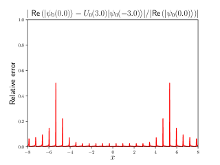
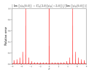
Figure 3: Relative error in the real and imaginary parts of the free path integral evolved wave packet from $t=-3$ to $t=0$.

These comparisons indicate that both the time steps and resolution are sufficiently small to evolve the free wave packet for $t=3.0$

In these calculations there was no attempt at efficiency; however because of the analytic expressions for the one-step probabilities, the one-step probabilities were computed on the fly in order to avoid storing large matrices. The resolution was chosen to be sufficiently fine to accurately represent the initial wave packet.

The next figure illustrates the effect of the potential on the evolution of the wave function. Figure 4 compares the real and imaginary parts of the scattering wave function $\langle x|\psi_{i}(0.0)\rangle=\langle x|\Omega(-3.0)|\psi_{i0}(0.0)\rangle$ (dotted line) at time $t=0.0$ to the initial wave packet $\langle x|\psi_{i0}(t=0.0)\rangle$ at $t=0.0$. The parameters used for this computation are $\Delta_{t}=0.1$, $\delta_{x}=0.01$ and $x\in[-25.0,25.0]$, which are the same parameters used to produce figures 2 and 3. The functions are calculated at the midpoint of each finite interval. Figure 4 shows the change in phase as the interaction is turned on. The dashed lines in both panels represent the initial wave packet, while the dotted lines represent the interacting wave packet.

These calculations approximate the incident scattered wave function at the collision time $(t=0.0)$. As discussed in section 2, the exact incident wave function at $t=0.0$ (or any common time) is needed to compute the differential cross section. These figures show that both the free and interacting $t=0.0$ wave functions occupy approximately the same volume, (about 20 units) which shows that using $\Omega(t)$ to calculate the scattering wave function eliminates spreading of the wave function. At time $t=0.0$ the phase of the incident wave is more dominantly shifted in the forward (right) side of the wave packet, which has spent the most time interacting with the interaction. This why these wave functions do not look like separated transmitted and reflected waves.

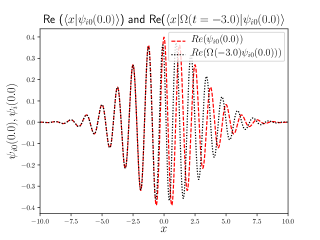
Figure 4: Shift in the phase of the real and imaginary parts of the incident wave packet at the collision time $t=0.0$

One of the complications of performing scattering calculations using real time path-integral methods is that the final expression for the transition matrix elements involves several approximations that need to be tested for convergence. With the potential turned on it is important to check that (1) the volume $[-25.0,25.0]$ is sufficiently large, the time step $\Delta t=0.1$ is sufficiently small, the resolution $\delta_{x}=0.01$ is sufficiently small, the total time $t=3.0$ is sufficiently large, and the calculation is stable with respect to changing the sample point $y_{i}$ in the interval $I_{i}$. The plots in figures 5-10 investigate the sensitivity of the time $t=0.0$ interacting wave functions to variations of the parameters used in the calculations shown in figure 4.

Note that all of the calculations assume that the evolved wave functions vanish on the half infinite intervals. This is justified both graphically and because the wave packet remains square integrable.

The Trotter product formula is justified in the small time step limit. The calculations illustrated in figure 4 used a time step $\Delta_{t}=0.1$. Figure 5 compares the real and imaginary parts of the scattered wave function $\langle x|\psi_{i}(0.0)\rangle=\langle x|\Omega(-3.0)|\psi_{i0}(0.0)\rangle$ using a time step size of $\Delta_{t}=.1$ (dashed curve) with corresponding calculations using a time step of half the size, $\Delta_{t}=.05$ (dotted curve). The plots of the real and imaginary parts of the scattered $t=0$ wave functions for $\Delta_{t}=.1$ and $\Delta_{t}=.05$ fall on top of each other. This indicates that the time resolution $\Delta_{t}$ is sufficiently fine for this calculation

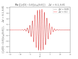
Figure 5: Plots of the real and imaginary parts of the time $t=0$ scattered wave packet calculated using Trotter time steps of $\Delta t=0.1$ and $\Delta t=0.05.$

While the Trotter approximation requires a sufficiently small time step, an accurate approximation of the wave operators requires a sufficiently large time. The initial choice of the approximating $\Omega_{-}:=\lim_{t\to-\infty}\Omega(t)$ by $\Omega(-3.0)$ was determined by examining the range of the potential and width and speed of the wave packet. Graphical methods indicated that the incident wave packed was still in the asymptotic region at $t=-3$. Figure 6 shows the effect of increasing the time from $t=3.0$ to $t=6.0$, keeping the size of the time step $\Delta_{t}=0.1$ constant, on the real and imaginary parts of the calculated scattering wave function. The plots of the wave functions for $t=-3.0$ (dashed curve) and $t=-6.0$ (dotted curve) fall on top of each other. This suggests that $t=3.0$ is sufficient for convergence.

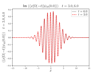
Figure 6: Plots of the real and imaginary parts of the scattered wave packet using approximate wave operators evaluated at $t=-3.0$ and $t=-6.0$.

The other limit used in this formulation of the path integral is the decomposition of the volume at each time slice into sufficiently small intervals. The spatial resolution of the intervals that define the cylinder sets should be sufficiently small that the wave function is effectively constant on them. The required resolution must be small due to the oscillating nature of the wave function, Figure 7 shows the effect of increasing the spatial resolution from 5000 intervals ($\delta_{x}=0.01$, dashed curves) to 10000 intervals ($\delta_{x}=0.005$, dotted curves) on the real and imaginary parts of the scattering wave function. In these calculations $\Delta_{t}=0.1$, $t=3.0$ and the interval is $[-25.0,25.0]$. Again the curves for the real and imaginary part of the wave function fall on top of each other. This indicates that for this problem a spatial resolution $\delta_{x}=.01$ (5000 intervals)) is sufficient for convergence.

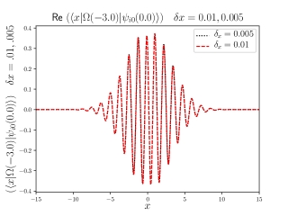
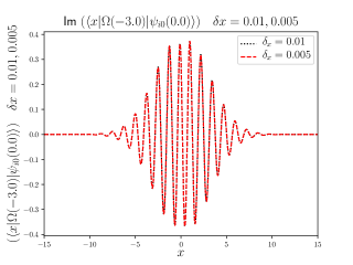
Figure 7: Plots of the real and imaginary parts of the scattered wave packet using cylinder sets with spacial resolutions of $0.01$ and $0.005$.

While the previous plots suggest that wave functions vanish outside of the volume $[-25.0,25.0]$, it is still important to check that the results are stable with respect to increasing the active volume of the calculation. Figure 8 compares calculations of the real and imaginary parts of the wave function where the volume is changed from $[-25.0,25.0]$ (dotted curves) to $[-50.0,50.0]$ (dashed curves) keeping $\delta_{x}=0.01$, $\Delta_{t}=0.1$, and $t=3.0$ Again, the calculations indicate the volume $[-25.0,25.0]$ is sufficient for convergence.

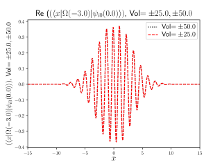
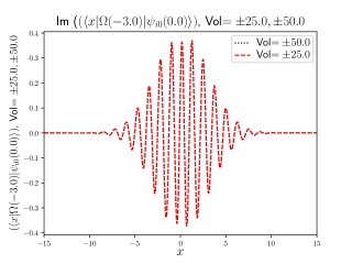
Figure 8: Plots of the real and imaginary parts of the scattered wave packet computed in the regions $[-25.0,25.0]$ and $[-50.0,50.0]$.

The size of the spatial intervals, $\delta x$, should be sufficiently small that the potential and initial wave free wave packet are approximately constant on the intervals. Figure 9 compares calculations where the potential is evaluated at the center or left endpoint of each interval for $\delta x=0.01$. Figure 9 shows the real and imaginary parts of the wave function, where the sample points are at the left (dash-dot line) and the center (dashed line) of the interval. This tests whether the potential is locally constant on each interval. These graphs show a small shift in the overall phase of the wave function. Figure 10 repeats the calculations shown in Figure 9 by increasing the resolution by a factor of 2. These figures show a corresponding reduction in the difference between the two curves. The conclusion is that the calculations in figure 4 seem to be most sensitive to the choice of the position in each interval used to evaluate the potential. This sensitivity may be due to large slope near the edges of the Gaussian potential shown in figure 1.

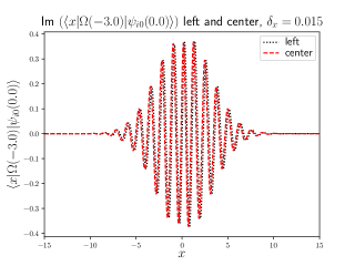
Figure 9: Plots of the real and imaginary parts of the scattered wave packet with the potential evaluated the at the center or left end of each interval for $\delta x=0.01$.

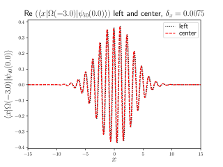
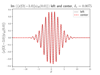
Figure 10: Plots of the real and imaginary parts of the scattered wave packet with the potential evaluated the at the center or left end of each interval for $\delta x=0.005$.

The goal of this work is to determine if these scattering wave functions can be used to calculate sharp-momentum transition matrix elements. Because the limits in the Trotter product formula are strong limits, the initial momentum was replaced by a narrow wave packet. To test the effect of the smearing, the sharp-momentum Born approximation is compared to the Born approximation where the initial sharp momentum state is replaced by a Gaussian delta function of width .25, which was used in the calculations above.

This comparison is illustrated in figure 11. The solid curve shows the Gaussian approximation to a delta function with width $\Delta p=.25$. The dotted curve shows the potential with initial momentum $p=5.0$, as a function of the final momentum. The dashed curve shows the same potential with the initial momentum replaced by the Gaussian delta function state centered at $p=5.0$ as a function of the final momentum.

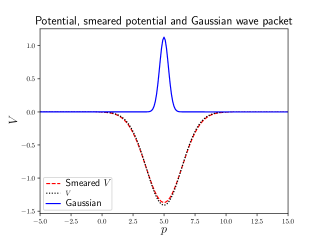
Figure 11: Plots of the delta function normalized Gaussian, the exact Born approximation to $T$, and the Born approximation smeared with the initial Gaussian wave packet.

The figure shows a small decrease in the matrix elements due to the smearing near the on-shell value.

As another test of the numerical convergence, the smeared Born approximation $\langle p|V|\Psi_{i0}(0)\rangle$ is compared to $\langle p|V\Omega_{0}(V=0,t=-3.0)|\Psi_{i0}(0.0)\rangle$, where the potential is turned off to compute $\Omega_{0}(-3.0)$. In this calculation $\delta x=0.01$ and $\Delta t=0.1$. This comparison is shown in figure 12. The imaginary part of $\langle p|V\Omega_{0}(V=0,t=-3.0)|\Psi_{i0}\rangle$, shown in the solid line should vanish, while the real parts of $\langle p|V|\Psi_{i0}(0.0)\rangle$ (dotted line) and $\langle p|V\Omega_{0}(V=0,t=-3.0)|\Psi_{i0}(0.0)\rangle$ (dashed line), should agree. The figure shows that the calculation accurately approximates the smeared Born approximation.

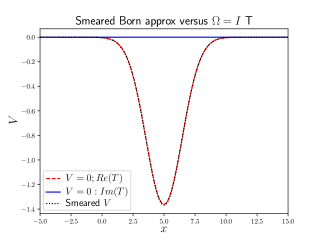
Figure 12: Plots of the exact smeared Born approximation, the real and imaginary parts of the Born approximation smeared against the wave packet computed using complex probabilities with V set to 0.

The approximate calculations give $V(x)\langle x|\Omega(-t)|\psi_{i0}\rangle$. The sharp-momentum transition matrix elements can be computed using a direct Fourier transform (13) or by integrating against Gaussian delta function with the desired final momentum (14). These two methods of calculation are compared in figure 13. In these calculations the $\Delta p$ of the final Gaussian is 0.25, which is the same value used in the initial Gaussian. The dashed curves show the real and imaginary parts of the smeared transition matrix elements computed using a direct numerical Fourier transform (dashed curves) compared to the curves which show the corresponding quantities that replace the final momentum by a Gaussian approximation to a delta function (dotted curves). For these calculations the time step was taken to be $\Delta t=0.025$, and $\delta_{x}=0.003$ which is smaller than the time step used in the calculations shown in figures 4-10. This is because the $T$-matrix calculations, which involve Fourier transforms or integration against oscillating wave packets, are more sensitive to the accuracy of the scattering wave functions. These figures show that both methods give results within a few percent of each other.

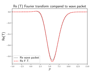
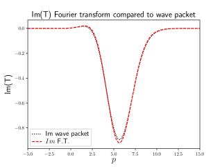
Figure 13: Plots of the real and imaginary parts of the $p=5.0$ half-shell T matrix computed by numerical Fourier transform and by smearing with a delta-function normalized Gaussian wave packet.

Figure 14 compares the real and imaginary parts of the smeared half-shell transition matrix elements (using the direct Fourier transform method (dotted curves) to sharp momentum half-shell transition matrix elements computed by numerically solving the Lippmann-Schwinger equation (dashed curves). As with the other calculation, errors are a few percent at the on-shell point. The comparison is between a sharp-momentum matrix element and a matrix element where the initial state is smeared with a narrow wave packet, so there will be some residual difference due to the smearing. The relative error for the real and imaginary parts are illustrated in figure 15. While the relative errors can be large, they are a few percent near the on shell point, $p=5.0$. All of the errors can be reduced by increasing the number of time steps and intervals.

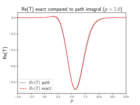
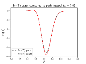
Figure 14: Plots of the real and imaginary parts of the half-shell transition matrix computed using the Fourier transform of the path integral calculation and by numerical solution of the Lippmann-Schwinger equation ($p=5.0$).

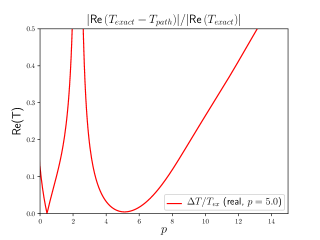
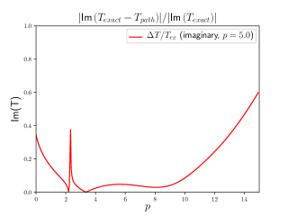
Figure 15: Plot of the absolute value of the relative error of the real and imaginary parts of the half-shell transition matrix path integral calculated using path integrals and the Lippmann-Schwinger equation where $p=5.0$ is the on-shell point.

In this one-dimensional problem there are two on-shell transition matrix elements corresponding to the transmitted wave and reflected wave. The calculations exhibited in the series of figures above are only for the transmitted wave. The on-shell matrix element for the reflected wave can be evaluated by changing the sign of the final momentum either in the Fourier transform on in the Gaussian approximation to the delta function. At this energy the transition matrix elements for the reflected wave are about five orders of magnitude smaller that those of the transmitted wave and are not reliable.

Phase shifts, transmission and reflection coefficients can be computed from the transition matrix elements. The results for $\Delta t=0.025$, $\delta_{x}=0.003$ between $-15.0$ and $15.0$, $\Delta p=0.25$ are shown below. For the Fourier Transform method the transition matrix elements are

$$\langle p|T|p\rangle=-8.04\times 10^{-01}-i8.17\times 10^{-01}\qquad\langle-p|T|p\rangle=-2.41\times 10^{-06}+i3.16\times 10^{-06}.$$

The phase shift for forward scattering is

$$\delta(p)=23.0^{\circ}.$$

A numerical calculation of the Lippmann-Schwinger equation gives a phase shift of $\delta(p)=25.4^{\circ}$ which is slightly larger than the computed phase shift. The phase shift for the reflected wave involves a ratio of two small numbers, both of which are smaller than computational errors, so it was not computed.

The transmission and reflection coefficient are

$$T=-0.027+i1.01\qquad R=3.03\times 10^{-6}+i3.99\times 10^{-6}$$

and the unitarity check gives

$$|T|^{2}+|R|^{2}=1.02$$

For the Gaussian approximate delta function the transition matrix elements are

$$\langle p|T|p\rangle=-7.85e^{-01}-i7.96e^{-01}\qquad\langle-p|T|p\rangle=-2.16e^{-06}+i3.35e^{-06}.$$

and the phase shifts are

$$\delta(p)=23.0^{\circ}\qquad\delta(-p)=0.0^{\circ}$$

which agree with the phase shifts calculated using the Fourier transform method. The reflection and transmission coefficients are

$$T=-1.59\times 10^{-04}+i0.986\qquad R=2.71\times 10^{-06}+i4.2\times 10^{-06}\\$$

and the unitarity check gives

$$|T|^{2}+|R|^{2}=0.972$$

Note that there are slight differences in the unitary checks for the two methods of computation.

For the calculations at $p=5.0$, the momentum was sufficiently high that the amplitude of the reflected wave was negligible relative to the transmitted wave.

Two additional calculations were performed at lower momenta ($p=2.5$ and $p=1.0$) that have larger amplitude reflected waves. For these calculations the width of the initial wave packet in momentum had to be sufficiently small so the spreading in position would not outrun the motion of the center of the wave packet. Decreasing the momentum width of the initial wave packet increases the spatial volume of the wave packet. This, along with the slower moving wave packet, increases the time that the particle feels the potential.

The results of these calculations are summarized in table III. The calculations in the table used the direct Fourier transform method, although it gives the same phase shifts as the Gaussian wave packet method. The calculations at $p=1.0$ used $15000$ spatial intervals between $-35.0$ and $35.0$ with a spatial resolution of $\delta_{x}=0.0047$. The total time was $t=45.0$ which was broken up into and $1000$ time steps of size $\Delta t=0.045$. The width of the initial wave packet was $\Delta p=0.1$.

The calculations at $p=2.5$ used $16000$ spatial intervals between $-15.0$ and $15.0$ with a spatial resolution of $\delta_{x}=.0019$. The total time was $t=7.0$ which was broken up into and $1000$ time steps of size $\Delta t=0.007$. The width of the initial wave packet was $\Delta p=0.2$. The phase shifts and unitarity checks for the three calculations are shown in table 2

Table 4: Phase shifts and unitarity checks

$p$	$\phi^{t}$	$\phi^{t}_{e}$	$\phi^{r}$	$\phi^{r}_{e}$	$R^{2}+T^{2}$
1	-49.1∘	-44.9∘	0.4∘	0.1∘	0.7
2.5	82.7∘	82.9∘	-74.8∘	-52.1∘	0.9
5.	23.0∘	25.4∘	0.0∘	0.0∘	1.0

The half-shell transition matrix elements for these two momenta are shown in figures 16-19. The real and imaginary parts of the calculated $p=1.0$ half-shell transition matrix elements are compared to the same quantities by numerically solving the Lippmann-Schwinger equation in figure 16. The path integral calculation reproduces the qualitative features of the solution of the Lippmann Schwinger equation. The corresponding relative errors for these two calculations are shown in figure 17. The relative errors are between 0.1 and 0.2 near the on-shell point.

These lower energy calculations required larger volumes and more time steps than the calculation at $p=5.0$, resulting in a much slower convergence.

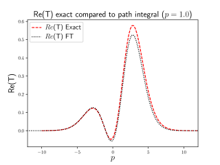
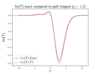
Figure 16: Plots of the real and imaginary parts of the half-shell transition matrix computed using the Fourier transform of the path integral calculation and by numerical solution of the Lippmann-Schwinger equation ($p=1.0$).

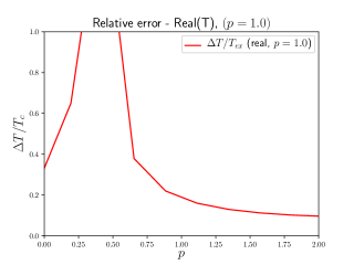
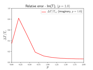
Figure 17: Plot of the absolute value of the relative error of the real and imaginary parts of the half-shell transition matrix path integral calculated using path integrals and the Lippmann-Schwinger equation where $p=1.0$ is the on-shell point.

The real and imaginary parts of the half-shell transition matrix elements for $p=2.5$ computed with the path integral and Lippmann Schwinger equation are compared in figures 18 and 19. The real part of the transition matrix element is almost a factor of 10 smaller than the imaginary part. In addition, from the graph, near the on shell point $p=-2.5$ the real and imaginary parts of the transition operator are near 0 so the calculation of the phase shift, which for the reflected wave is a function of the ratio of these two small quantities, is dominated by computational errors.

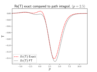
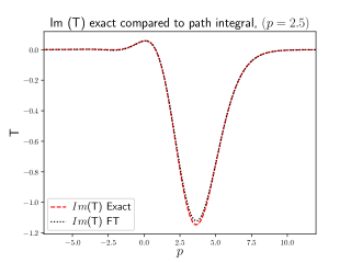
Figure 18: Plots of the real and imaginary parts of the half-shell transition matrix computed using the Fourier transform of the path integral calculation and by numerical solution of the Lippmann-Schwinger equation ($p=2.5$).

The corresponding relative error in the real and imaginary parts of the transition matrix at $p=2.5$ are shown in figures 19. They are about $.03$ at the on shell point.

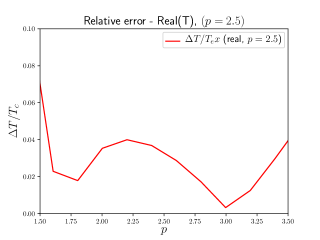
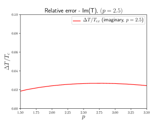
Figure 19: Plot of the absolute value of the relative error of the real and imaginary parts of the half-shell transition matrix path integral calculated using path integrals and the Lippmann-Schwinger equation where $p=5.0$ is the on-shell point.

The results indicate that lower energy calculations require more computational resources than the higher energy calculations. There are a number of reasons for this. The slow moving wave packet must outrun the negative spreading of the initial wave packet. In addition, the higher momentum resolution needed for low-energy calculations increases the relevant volume that needs to be decomposed into products of intervals. The exhibited calculations, especially the lower energy calculations, already involved iterating large matrices ($15000\times 15000$). Fortunately these matrices do not have to be stored. The calculations are approximations in the sense that they mathematically converge to the exact result. This means that in principle they can be improved by using more computational resources (larger matrices and more time steps). We did not attempt to go beyond calculations of this size for $p=1.0$ and $p=2.5$ in part because with the brute force computational methods used in this work, small increases in resolution result in much larger calculations. For this reason convergence is slow and it makes sense to first investigate methods to improve the efficiency of the calculations, rather than to continue investigating the limits of these inefficient methods. It is clear from the above discussions, that calculations of zero-energy observables, like scattering lengths, would be very difficult. This is because it would be necessary to use narrow wave packets in momentum that would result require large volumes.

VII Summary and Conclusions

This work demonstrated both the feasibility and challenges of performing scattering calculations using real-time path integrals.

The exhibited calculations are based on a reinterpretation of the path integral as the expectation of a potential functional with respect to a complex probability distribution on a space of paths. The space of paths is constructed by dividing the total time into a large number of small time slices. At each time slice space is divided up into a large number of small windows, including two semi-infinite windows. The space of paths can then be decomposed into disjoint equivalence classes where equivalent paths pass thorough the same intervals at each time slice.

A complex probability is assigned to each equivalence class. It is constructed by decomposing the propagation of a free quantum mechanical system into a sum of parts associated with each equivalence class. Interactions are introduced by considering the effects of the potential at each window. Mathematically the time evolution of an initial wave packet is represented by an average of a path-dependent potential functional on the space of paths with respect to the complex probability distribution. The virtue of this method is that it is a real approximation in the sense that it converges to a global solution of the Schrödinger equation.

For the convergence of the calculations the equivalence class of paths must be sufficiently fine that the potential locally constant on each spatial volume element. In addition, the time steps must be sufficiently small for the Trotter product formula to converge. The fact that the complex probabilities are largely supported on continuous paths means that for smooth short-range potentials the relevant volume is finite.

One difficulty is the large number of equivalence classes. Each equivalence class can be represented as the product of $N$ one-step classes for each time step. This can be used to make an approximate factorization of the $N$-time step complex probability as a product of $N$ one-time-step probabilities. This approximation replaces the sum over the large number of equivalence classes by computing powers of a large matrix, which was used in the calculations. In this representation the contribution of each equivalence class is approximated by a particular sequence of products of matrix elements. For example, if $M_{mn}$ represents the one step probability matrix, the product of numbers

$$M_{n_{0}n_{1}}M_{n_{1}n_{2}}\cdots M_{n_{19}n_{20}}$$ (66)

is approximately the complex probability for passing through the sequence of windows $I_{n_{20}}$ at time $t_{1}$, $I_{n_{19}}$ at time $t_{2},\cdots$. This factorization represents a tremendous increase in efficiency - by using matrix algebra to treat a large number of equivalence classes of paths in parallel. Computationally this looks like replacing the path integral by successive applications of a transfer matrix to an initial state, except in this case it is possible to identify and extract the contribution of each cylinder set of paths to the free-particle time-evolution operator.

The scattering calculations were performed by approximating Møller wave operators Møller (1945) applied to normalizable wave packets. This has the advantage of removing wave packet spreading effects from the scattering calculations. The relevant volume is the region where the particles interact. It is determined by the range of the interactions and size of the free wave packets. One possible strategy to improve the efficiency would be to reduce the size of the active volume by building some of the asymptotic properties of scattering wave function into the free wave functions. This is essential for long-range potentials Dollard (1964) Mulherin and Zinnes (1970)Busalev and Matveev (1970), but similar methods could be applied to short range potentials.

The $p=5.0$ calculations presented in this paper formally involve applying the $30^{th}$ power of a $5000\times 5000$ matrix to a fixed vector (for the transition matrix element calculations the $100^{th}$ power of a $10000\times 10000$ matrix). This corresponds to averaging over $5000^{30}$ (resp $(10000)^{100}$) equivalence classes of paths. Because the one-step probabilities could be computed analytically, accurately and efficiently, matrix elements could be computed on the fly, which means that the computer storage required for these calculations amounted to storing few complex vectors of length 5000(10000). One of the surprising aspects of these calculations is the stability of the sums over the complex probabilities.

The $p=5.0$ calculations presented were performed in minutes on a desktop computer. The $p=1.0$ and $p=2.5$ calculations required larger space-time volumes and more time steps and took more than a day on the same computer. In terms of the number of cylinder sets the $p=1.0$ calculations presented used the equivalent of $(15000)^{1000}$ cylinder sets while the $p=2.5$ calculations used the equivalent of $(16000)^{1000}$ cylinder sets. As a result they took considerably longer. No attempt was made to be efficient. All intervals and time steps were taken to be the same size. This is the analog of computing a Riemann integral with equally spaced intervals. There is a great deal of freedom both in how to choose intervals and time slices that was not exploited. Some strategies that could be explored would be use more resolution of cylinder sets near classical paths. The structure of the potential could be used to determine and optimal decomposition of each time slice into intervals. The presented calculations simply applied the same matrix $N$ times to the initial vector. The application of the one-step probability matrix to a localized vector could be made more efficient by discarding small components of the resulting vector, reducing the size of the vector that must be stored for each time step. The one step complex probabilities approximate a unitary transfer matrix for free evolution, however exact unitarity is not forced on the resulting matrices. Designing the one step probability so the matrix is exactly unitary may reduce errors.

Beyond the numerical considerations, this framework is appealing in that the input is a potential functional $F[\gamma]$; this picture is retained both exactly and in approximation. This is in contrast to the usual path integral where the relevant weight functional formally looks like an action, but the terms that represent the time derivatives have no legitimate interpretation as derivatives in the Trotter product formula. In the MNJ formulation, these terms do not appear explicitly; they are contained in the expression for the one-step probabilities

While the calculations in this paper are motivated by the complex probability interpretation, the computational strategy can be understood directly from Feynman’s work. His path integral results in the kernel $K(x,t;x^{\prime},t^{\prime})$ of the time evolution operator (see equation (4.2) of Feynman and Hibbs (1965))

$$\langle x|\psi(t)\rangle=\int K(x,t;x^{\prime},t^{\prime})dx^{\prime}\langle x^{\prime}|\psi(t^{\prime})\rangle$$ (67)

This can be expressed as the product of propagation over many time steps (see equation (2.33) of Feynman and Hibbs (1965)) :

$$\langle x|\psi(t)\rangle=\int K(x,t;x_{1},t_{1})dx_{1}K(x_{1},t_{1};x_{2},t_{2})dx_{2}\cdots K(x_{N-1},t_{N-1};x_{N},t_{N})dx_{N}\langle x_{N}|\psi(t_{N})\rangle$$ (68)

If the time intervals $t_{j+1}-t_{j}$, are sufficiently small then

$$K(x_{j+1},t_{j+1};x_{j},t_{j})\approx K_{0}(x_{j+1},t_{j+1};x_{j},t_{j})e^{-iV(x_{j})(t_{j+1}-t_{j})}$$ (69)

where $K_{0}(x_{j+1},t_{j+1};x_{j},t_{j})$ is the free time-evolution kernel. This is justified by the Trotter product formula. Finally, if the integrals were replaced by numerical quadratures, this would become

$$\langle x|\psi(t)\rangle\approx\sum K_{0}(x,t;x_{1n_{1}},t_{1})e^{-iV(x_{1n_{1}})(t-t_{1})}\Delta_{x_{1n_{1}}}K_{0}(x_{1n_{1}},t_{1};x_{2n_{2}},t_{2})e^{-iV(x_{2n_{2}})(t_{1}-t_{2})}\Delta_{x_{2n_{2}}}\cdots\times$$

$$K_{0}(x_{(N-1)n_{N-1}},t_{N-1};x_{Nn_{N}},t_{N})e^{-iV(x_{Nn_{N}})(t_{N-1}-t_{N})}\Delta_{x_{Nn_{N}}}\langle x_{N}|\psi(t_{N})\rangle\Delta_{x_{2n_{2}}}.$$ (70)

The approximation

$$K_{0}(x_{1n_{1}},t_{1};x_{2n_{2}},t_{2})\Delta_{x_{2n_{2}}}\approx\int_{x_{2n_{2}}-\Delta_{x_{2n_{2}}}/2}^{x_{2n_{2}}+\Delta_{x_{2n_{2}}}/2}K_{0}(x_{1n_{1}},t_{1};x,t_{2})dx$$ (71)

corresponds to the one-step probability used in this work. If this replacement is made in (70) the result is equivalent to (46). The important features to emphasize are (1) because of the small time steps, the potential can be factored out and evaluated at one of the quadrature points and (2) the free particle kernel is known. It is these two features that make non-trivial calculations possible.

The short time kernel

$$K_{0}(x,t;x^{\prime},t+\Delta t)$$

can be computed analytically leading to the following unitary kernel for the approximate transfer matrix:

$$TM(x,t;x^{\prime},t+\Delta t)=K_{0}(x,t;x^{\prime},t+\Delta t)e^{-iV(x^{\prime})}$$

$$P(x^{\prime}\to x,dx,\Delta t):=dxTM(x,t;x^{\prime},t+\Delta t)$$

can be interpreted as a one-step complex probability for a particle initially at $x^{\prime}$ to end up within $dx$ of $x$ in time $\Delta t$. A direct numerical calculation with this kernel may be more efficient that the brute force calculation illustrated above.

The interesting question is how this method scales to more particles or fields? While it is difficult to answer this question without performing a test calculation and taking advantage of efficiencies, For small time steps the Trotter formula justifies the replacements

$$e^{-i(\sum H_{i}+\sum V_{ij})\Delta t}\to\prod e^{-iH_{i}\Delta t}e^{-i\sum V_{ij}\Delta t}\to\prod e^{-iH_{i}\Delta t}\prod e^{-iV_{ij}\Delta t}.$$

In this form there are more products for a given time step, but the non-trivial products only involve exponentials of single pairwise potentials or one-body free propagators. Each of these operators, $e^{-iH_{i}\Delta t}$ or $e^{-iV_{ij}\Delta t}$, only act on the variables associated with particle $i$ or particles $i$ and $j$ in the many-body wave function. This suggest that the non-trivial part a few-body calculation scales with the number of interacting pairs. There are other factors, in that both the relevant volume and interaction time will increase as more particles are added. In addition serious challenges with storing the vector representing the evolved many-body wave function must be overcome..

The exhibited one-dimensional calculations are of comparable difficulty to computing three-dimensional two-body scattering calculations using partial waves in the center of mass frame. Time-dependent methods based on numerical computation of wave operators have been successfully applied to treat-three body $n$-$D$ breakup with strong $+$ Coulomb interactions Kröger and Slobodrian (1984). These calculation suggest that with some improvements in efficiency that real path integral scattering calculations involving two or three particles might be possible.

While this work demonstrates that scattering observables can be directly computed using real-time path integrals, the calculations used in this work cannot compete with conventional computational methods. These methods may provide a useful laboratory for investigating the efficiency of different approximation methods for treating real time evolution, which is needed for scattering calculations on a quantum computer.

Conceptually, the one-step probability multiplied by the one-step potential functional, $e^{-iV(y_{i})\Delta t}$, which is the key to the computational method, is essentially a transfer matrix, which is a unitarized version of using the Hamiltonian to solve the Schrödinger equation for finite time by taking many small time steps. This has a lot in common with evolving a product of smeared field operators with the Heisenberg equations of motion. Also, the one-step complex probability is essentially free propagation over short time, which is also well understood in the field-theory case.

One of the authors (WP) would like to acknowledge the generous support of the US Department of Energy, Office of Science, grant number DE-SC0016457 who supported this research effort.

References

- Feynman (1948) R. Feynman, Reviews of Modern Physics 2, 367 (1948).
- Feynman and Hibbs (1965) R. Feynman and A. R. Hibbs, Quantum Mechanics and Path Integrals (McGraw-Hill, USA, 1965).
- Muldowney (2012) P. Muldowney, A Modern Theory of Random Variation (Wiley, N.J., 2012).
- Nathanson and Jørgensen (2015) E. S. Nathanson and E. Jørgensen, Palle, J. Math. Phys. 56, 092102 (2015).
- Nathanson (2015) E. S. Nathanson, University of Iowa Thesis (2015).
- Richtmyer et al. (1947) D. Richtmyer, J. Pasta, and S. Ulam, LANL report LAMS 551 (1947).
- Metropolis and S. (1949) N. Metropolis and U. S., Journal of the American Statistical Association 44, 335 (1949).
- Luscher and Wolff (1990) M. Luscher and U. Wolff, Nuclear Physics B339, 222 (1990).
- Luscher (1986) M. Luscher, Comm. Math. Phys. 105, 153 (1986).
- Bing-Nan et al. (2016) L. Bing-Nan, L. T. A., D. Lee, and U. G. Meißner, Phys. Letters B 760, 309 (2016).
- Luu and Savage (2011) T. Luu and M. J. Savage, Phys. Rev. D. 83, 114508 (2011).
- Aiello and Polyzou (2016) G. J. Aiello and W. N. Polyzou, Phys. Rev. D 93, 056003 (2016).
- Faddeev and Slavnov (1980) L. D. Faddeev and A. A. Slavnov, Gauge Fields, Introduction to Quantum Theory, vol. I (Benjamin Cummings, Reading, Mass., 1980).
- Rosenfelder (2009) R. Rosenfelder, Phys. Rev. A 79, 012701 (2009).
- Carron and Rosenfelder (2011) J. Carron and R. Rosenfelder, Phys. Letters. A 375, 3781 (2011).
- Campbell et al. (1975) W. B. Campbell, P. Finkler, C. E. C. E. Jones, and M. N. Misheloff, Phys. Rev. D 12, 2363 (1975).
- Henstock (1963) R. Henstock, Theory of Integration (Butterworths, London, 1963).
- Bartle (2001) R. G. Bartle, A modern theory of integration, vol. 32 (American Mathematical Society, Providence, RI, 2001).
- Gill and Zachary (2008) T. Gill and W. Zachary, Real Analysis Exchange 34, 1 (2008).
- Reed and Simon (1980) M. Reed and B. Simon, Methods of Modern Mathematical Physics, vol. I (Academic Press, San Diego, 1980).
- Nathanson and Jørgensen (2017) E. S. Nathanson and E. Jørgensen, Palle, J. Math. Phys. 58, 122101 (2017).
- Dollard (1964) J. D. Dollard, J. Math. Phys. 5, 729 (1964).
- Dollard and Friedman (1978) J. D. Dollard and C. N. Friedman, Annals Phys. 111, 251 (1978).
- Haag (1958) R. Haag, Phys. Rev. 112, 669 (1958).
- Ruelle (1962) D. Ruelle, Helv. Phys. Acta. 35, 147 (1962).
- Lippmann and Schwinger (1950) B. A. Lippmann and J. Schwinger, Physical Review 79, 409 eq 1.63 (1950).
- Nelson (1964) E. Nelson, Journal of Mathematical Physics 5, 332 (1964).
- Abramowitz and Stegun (1964) M. Abramowitz and I. Stegun, Handbook of Mathematical Functions, vol. 55 (National Bureau of Standards, Washington DC., 1964).
- Møller (1945) C. Møller, Det. Kggl. Danske Videnskaberbernes Selskab, Matematisk-Fysiske Meddelelser 23(1) (1945).
- Mulherin and Zinnes (1970) D. Mulherin and I. I. Zinnes, J. Math. Phys. 11, 1402 (1970).
- Busalev and Matveev (1970) V. S. Busalev and V. B. Matveev, Theoret. and Math. Phys. 2, 266 (1970).
- Kröger and Slobodrian (1984) H. Kröger and R. J. Slobodrian, Phys. Rev. C. 30, 1390 (1984).