Resource Sharing of a Computing Access
Point for Multi-user Mobile Cloud Offloading
with Delay Constraints

Abstract

We consider a mobile cloud computing system with multiple users, a remote cloud server, and a computing access point (CAP). The CAP serves both as the network access gateway and a computation service provider to the mobile users. It can either process the received tasks from mobile users or offload them to the cloud. We jointly optimize the offloading decisions of all users, together with the allocation of computation and communication resources, to minimize the overall cost of energy consumption, computation, and maximum delay among users. The joint optimization problem is formulated as a mixed-integer program. We show that the problem can be reformulated and transformed into a non-convex quadratically constrained quadratic program, which is NP-hard in general. We then propose an efficient solution to this problem by semidefinite relaxation and a novel randomization mapping method. Furthermore, when there is a strict delay constraint for processing each user’s task, we further propose a three-step algorithm to guarantee the feasibility and local optimality of the obtained solution. Our numerical results show that the proposed solutions give nearly optimal performance under a wide range of parameter settings, and the addition of a CAP can significantly reduce the cost of multi-user task offloading compared with conventional mobile cloud computing where only the remote cloud server is available.

1 Introduction

Mobile Cloud Computing (MCC) extends the capabilities of mobile devices to improve user experience[2][3][4]. Mobile users can offload tasks to the cloud, using abundant cloud resources to help them gather, store, and process data. However, the interaction between mobile devices and the cloud introduces some key challenges in the system design. For example, the decision on whether to offload tasks to the cloud needs to balance the tradeoff between energy consumption and computing performance. Furthermore, the communication delay between mobile users and the cloud needs to be taken into consideration [2].

With an aim to reduce the communication delay in task offloading, Mobile Edge Computing (MEC), as defined by the European Telecommunications Standards Institute (ETSI), is a distributed MCC system where computing resources are installed locally at or near the base station of a cellular network [5][6][7]. MEC shares similarities with micro cloud centers [8], cloudlets[9], cyber-foraging[10], and fog computing [11], except that the MEC computing servers are managed by a mobile service provider, which allows more direct control and resource management.

Similar to the concept of MEC, in this work, we use the general term computing access point (CAP), which refers to a wireless access point or a cellular base station with built-in computation capability. For example, CAPs may be provided by Internet service providers as a value-added service. Mobile devices that wish to offload a task first sends it to the CAP. The CAP may serve its conventional networking function and forward the task to the remote cloud server, or directly process the task by itself. The additional option of computation by the CAP reduces the need for access to the remote cloud server, and hence can potentially decrease the communication delay and also the overall energy and computation cost. However, the availability of CAP adds an extra dimension of variability for offloading decisions. Each task may be processed locally at the mobile device, at the CAP, or at the remote cloud server. Furthermore, both computation and communication resources need to be considered in different offloading choices. This makes optimizing the mobile task offloading decision even more challenging.

In this work, we study the interaction among multiple users, the CAP, and the cloud. In a multi-user scenario, to offload tasks, we need to allocate communication and computation resources among competing users. We jointly consider both the offloading decision and resource allocation among all users, with an aim to conserve energy and maintain service quality for all of them. For this joint optimization problem, an optimal offloading decision must take into consideration the computation and communication energies, computation costs, and communication and processing delays at all local user devices, as well as the resource constraints and capabilities of the CAP and the remote cloud. The contributions of this work are summarized as follows:

• We focus on jointly optimizing the offloading decisions as well as the computation and communication resource allocation for multiple mobile users with one CAP and one remote cloud server. We formulate the joint optimization problem to minimize a weighted sum of costs of energy, computation, and the maximum delay among all users. This results in a mixed integer programming problem. To solve this challenging problem, we first reformulate and transform the problem into a non-convex quadratically constrained quadratic program (QCQP) [12], which is still NP-hard in general. To obtain a solution to this problem, we then propose an efficient heuristic algorithm, termed shareCAP, based on semidefinite relaxation (SDR) [13] and a novel randomization mapping method.

• We further study the scenario where there is a strict processing deadline for each user’s task. With these additional delay constraints, the proposed shareCAP method can no longer be directly applied to find a solution due to the absence of a feasibility guarantee. To solve this more complicated optimization problem, we further propose a three-step algorithm named shareCAP-D, consisting of SDR, adaptive adjustment, and sequential tuning, to iteratively find a solution. We show that shareCAP-D guarantees a locally optimal solution.

• Through numerical study, by comparing with an optimal offloading policy obtained by exhaustive search, we demonstrate that the proposed shareCAP and shareCAP-D methods give nearly optimal performance under a wide range of parameter settings. Furthermore, we observe that the addition of a CAP can significantly reduce the energy and computational costs of the system, as compared with the conventional MCC where only the remote cloud server is available for task offloading.

The rest of this paper is organized as follows. Related works are reviewed in Section 2. In Section 3, we describe the system model for mobile cloud computing with a CAP and formulate the optimization problem. In Section 4, we transform our problem to a QCQP problem and solve it through the SDR approach. In Section 5, we further study the scenario with strict delay constraints. In Section 6, we extend our work to sum delays optimization. Numerical results are presented in Section 7, followed by conclusion in Section 8.

Notations: We denote by $\mathbf{a}^{T}$ and $\mathbf{A}^{T}$ the transpose of vector $\mathbf{a}$ and matrix $\mathbf{A}$, respectively. The notation $\mathrm{diag}(\mathbf{a})$ denotes the diagonal matrix with diagonal elements being elements of vector $\mathbf{a}$. The trace function of matrix $\mathbf{A}$ is denoted by $\mathrm{Tr}(\mathbf{A})$. We use $\mathbf{A}(i,j)$ to denote the $(i,j)\mathrm{th}$ entry of matrix $\mathbf{A}$. We use $\mathbf{A}\succeq 0$ to indicate that $\mathbf{A}$ is a positive semi-definite matrix.

2 Related Work

Many existing works study task offloading from mobile users to the local (or remote) processor in two-tier cloud systems. For a single mobile user offloading its entire application to the cloud, the authors of [14, 15, 16] presented different energy models to analyze whether or not to offload application to the cloud, and the tradeoff between energy consumption and computing performance was studied in [17, 18]. Furthermore, many studies have considered partitioning an application into multiple tasks. Among them, MAUI [19], Clonecloud [20], and Thinkair [21] are systems proposed to enable a mobile device to offload tasks to the cloud. These works focus on the implementation of offloading mechanisms from the mobile device to the cloud, and the discussion on optimizing the offloading decisions was limited. In [22] and [23], heuristic offloading policies were proposed for a mobile user with sequential tasks. In [24, 25, 26], the problem of cloud offloading for a mobile user with dependent tasks was studied. In [27], offloading a mobile user’s tasks in an intermittently connected cloud system was considered. The impact of mobility was considered in [28], where the authors proposed an opportunistic offloading algorithm. All of the studies above focus on a single mobile user.

Task offloading by multiple mobile users have been considered in [29, 30, 31, 32, 33, 34, 35, 36, 37], where each user has a single application or task to be offloaded to the cloud in its entirety. In [29, 30, 31], the authors considered optimizing offloading decisions, aiming to maximize the revenue of the mobile cloud service providers under a fixed resource usage per user. The cooperation among selfish service providers to improve the revenue was further studied in [31]. The authors of [32, 33] studied the allocation of radio and computation resources in the scenario where all tasks are always offloaded. The joint optimization of offloading decision and communication and computation resources for system utility maximization was considered in [34], where where the number of tasks that can be offloaded is limited by the transmission bandwidth; a heuristic algorithm was proposed to obtain the resource allocation and offloading decision sequentially. Game theoretic approaches were adopted in [35, 36, 37] to study decentralized decision control in systems where offloading decisions are made by mobile users as selfish players. However, these game theoretic works focus on the offloading decisions for each user without considering the allocation of communication and computation resources. Furthermore, a multi-user scenario where each user has multiple independent tasks was considered in [38], where the offloading decision algorithm were proposed by minimizing the weighted cost of energy consumption and worst-case offloading delay. The authors of [39] considered a mobile device cloud, which is composed purely of proximal mobile devices, and a task scheduling mechanism was proposed for concurrent application management. Coordination of local mobile devices forming a mobile cloud has been studied in [40]. All of the studies above focus on a two-tier cloud network consisting of only mobile users and another tier of local or remote processors.

The three-tier network consisting of mobile users, a local computing node (e.g., cloudlet or CAP), and a remote cloud server has been studied in [41, 42, 43, 44, 45]. Without considering resource allocation, centralized heuristic algorithms for offloading decisions were proposed in [41, 42, 43], while a game theoretic approach was considered to distributedly obtain the offloading decision in [44]. Despite these works, the joint optimization of the offloading decision and the allocation of computation and communication resources for a general three-tier system has not been investigated before. The joint optimization problem is much more complicated to solve, because the offloading decision and resource allocation are inter-dependent.

In our recent work [45], a multi-user scenario where each user has multiple independent tasks was considered for joint optimization of offloading and allocation of communication and computation resources. The differences of this work and [45] are as follows: 1) The problem structures are different, leading to different problem formulations and solution approaches; 2) For the single-task per user case studied in this paper, we propose a low-complexity algorithm that is shown to achieve nearly optimal performance. This combined advantage in both the complexity and performance cannot be achieved by the algorithm proposed in [45]; 3) In this work, we further study the scenario where a strict processing deadline is imposed on each user’s task, which cannot be addressed by the solution approach proposed in [45].

3 System Model and Problem Formulation

In this section, we first introduce the model of mobile cloud computing with a CAP, detailing the costs of processing locally, at the CAP, and at the cloud. We then explain the joint offloading decision and resource allocation optimization problem to minimize a weighted sum cost.

3.1 System Model

3.1.1 Mobile Cloud with CAP

Consider a cloud access network with $N$ mobile users, one CAP, and one remote cloud server, as shown in Fig. 1. The CAP is a wireless access point (or a cellular base station) with built-in computation capability that may be provided by Internet service providers as a value-added service. Instead of just serving as a relay to always forward received tasks from users to the cloud, the CAP also has the capability to process user tasks subject to its resource constraint. We denote the set of all users by $\mathcal{N}=\{1,...,N\}$. Each mobile user has one task to be either processed locally or offloaded to the CAP, and the CAP determines whether to process each received task by itself or further offload it to the cloud for processing. Since there are multiple tasks offloaded to the CAP and some of them are processed by the CAP, we need to further allocate the communication and computation resources available at the CAP.

Figure 1: System model

We assume that all tasks are available at time zero. This is similar to many existing studies [15, 16, 17, 18, 33, 35, 36, 37, 34]. If the tasks arrive dynamically in time, we may apply our model and the proposed solution in a quasi-static manner, where the system processes the tasks in batches that are collected over time intervals [46].

3.1.2 Offloading Decision

Denote the offloading decisions for user $i$ by $x^{l}_{i},x^{a}_{i},x^{c}_{i}\in\{0,1\}$, indicating whether user $i$’s task is processed locally, at the CAP, or at the cloud, respectively. The offloading decisions are constrained by

$$x^{l}_{i}+x^{a}_{i}+x^{c}_{i}=1,\ i\in\mathcal{N}.$$ (1)

Notice that only one of $x^{l}_{i}$, $x^{a}_{i}$, and $x^{c}_{i}$ for user $i$ can be $1$.

3.1.3 Cost of Local Processing

The input data size, output data size, and processing cycles of user $i$’s task are denoted by $D_{{\textrm{in}}}(i)$, $D_{{\textrm{out}}}(i)$, and $Y(i)$, respectively. Similar to [16, 17, 18, 33, 35, 36, 37, 34], we assume that these quantities are known, which may be achieved by applying a program profiler [19, 20, 21]. We assume that the additional instructions required for remote processing can be downloaded directly by the CAP or the cloud via their access to a high-capacity wired network. When the task is processed locally, the processing energy is denoted by $E^{l}_{i}$ and the processing time is denoted by $T^{l}_{i}$.

3.1.4 Cost of CAP Processing

For user $i$’s task being offloaded to the CAP, we denote the energy consumed by wireless transmission (to the CAP) and reception (from the CAP) at user $i$ by $E^{t}_{i}$ and $E^{r}_{i}$, respectively. We further denote the uplink and downlink transmission times between user $i$ and the CAP by $T^{t}_{i}=D_{{\textrm{in}}}(i)/(\eta^{u}_{i}c^{u}_{i})$ and $T^{r}_{i}=D_{{\textrm{out}}}(i)/(\eta^{d}_{i}c^{d}_{i})$, respectively, where $c^{u}_{i}$ and $c^{d}_{i}$ are uplink bandwidth and downlink bandwidth allocated to user $i$, and $\eta_{i}^{u}$ and $\eta_{i}^{d}$ are the spectral efficiency of uplink and downlink transmission between user $i$ and the CAP, respectively. Furthermore, $c^{u}_{i}$ and $c^{d}_{i}$ are limited by the uplink bandwidth $C_{\textrm{UL}}$ and downlink bandwidth $C_{\textrm{DL}}$ as follows

$$\sum_{i=1}^{N}c^{u}_{i}\leq C_{\mathrm{UL}},$$ (2)

and

$$\sum_{i=1}^{N}c^{d}_{i}\leq C_{\mathrm{DL}}.$$ (3)

Since some uplink and downlink transmissions may overlap with each other, there is also a total bandwidth constraint

$$\sum_{i=1}^{N}(c^{u}_{i}+c^{d}_{i})\leq C_{\mathrm{Total}}.$$ (4)

If this task is processed by the CAP, denote its processing time by $T^{a}_{i}=Y(i)/f^{a}_{i}$, where $f^{a}_{i}$ is the assigned processing rate, which is limited by the total processing rate $f_{A}$ at the CAP as

$$\sum_{i=1}^{N}f^{a}_{i}\leq f_{A}.$$ (5)

The usage cost associated with the CAP processing user $i$’s task is denoted by $C_{i}^{a}$. The usage cost may depend on the data size and processing cycles of a task, as well as the hardware and energy cost to maintain the CAP. Detailed modeling of the usage cost is outside the scope of this work. Here we simply assume that $C^{a}_{i}$ is given for all $i$.

3.1.5 Cost of Cloud Processing

TABLE I: Notation and corresponding description.

Notation	Description
$D_{{\textrm{in}}}(i)$, $D_{{\textrm{out}}}(i)$	input data size and output data size of
	user $i$’s task
$Y(i)$	processing cycles of user $i$’s task
$E^{l}_{i}$	local processing energy of user $i$’s task
$E^{t}_{i}$, $E^{r}_{i}$	uplink transmitting energy and
	downlink receiving energy of user $i$’s
	task to and from the CAP
$T^{l}_{i}$, $T^{a}_{i}$, $T^{c}_{i}$	local processing time, CAP processing
	time, and cloud processing time of
	user $i$’s task
$T^{t}_{i}$, $T^{r}_{i}$	uplink transmission time and
	downlink transmission time of
	user $i$’s task between the mobile user
	and the CAP
$T^{ac}_{i}$	transmission time of user $i$’s task
	between the CAP and the cloud
$C_{\textrm{UL}}$, $C_{\textrm{DL}}$	uplink bandwidth and downlink
	bandwidth for transmission between
	mobile users and the CAP
$C_{\textrm{Total}}$	total transmission bandwidth between
	mobile users and the CAP
$c^{u}_{i}$, $c^{d}_{i}$	uplink bandwidth and downlink
	bandwidth assigned to user $i$
$\eta_{i}^{u}$, $\eta_{i}^{d}$	spectral efficiency of uplink and
	downlink transmission between user $i$
	and the CAP
$C^{a}_{i}$, $C^{c}_{i}$	CAP usage cost and cloud usage cost
	of user $i$’s task
$r^{ac}$	transmission rate for each user
	between the CAP and the cloud
$f^{c}$	cloud processing rate for each user
$f_{A}$	total CAP processing rate
$f^{a}_{i}$	CAP processing rate assigned to user $i$
$\alpha$	weight of the CAP usage cost
$\beta$	weight of the cloud usage cost
$\rho_{i}$	weight of the energy consumption of
	user $i$’s task

If a task is further offloaded to the cloud from the CAP, besides all the costs mentioned above (except $T^{a}_{i}$ and $C^{a}_{i}$ related to the task processing cost by the CAP), there is an additional transmission time between the CAP and the cloud, denoted by $T^{ac}_{i}=(D_{{\textrm{in}}}(i)+D_{{\textrm{out}}}(i))/r^{ac}$, where $r^{ac}$ is the transmission rate between the CAP and the cloud. Also, the cloud processing time is denoted by $T^{c}_{i}=Y(i)/f^{c}$, where $f^{c}$ is the cloud processing rate for each user. The rate $r^{ac}$ is assumed to be a pre-determined value regardless of the number of users. This is because the CAP-cloud link is likely to be a high-capacity wired connection as compared with the limited wireless links between the mobile users and the CAP, thus there is no need to consider bandwidth sharing among the users. Similarly, $f^{c}$ is also assumed to be a pre-determined value because of the high computational capacity and dedicated service of the remote cloud server. Thus, $T^{ac}_{i}$ and $T^{c}_{i}$ only depend on task $i$ itself. Finally, the cloud usage cost of processing user $i$’s task at the cloud is denoted by $C^{c}_{i}$.

The above notations are summarized in Table I.

3.2 Problem Formulation

Our goal is to reduce the mobile users’ energy consumption and maintain the service quality to their tasks. To do so, we define the total system cost as the weighted sum of total energy consumption, the costs to offload and process all tasks, and the corresponding maximum transmission and processing delays among all users. We aim to minimize the total system cost by jointly optimizing the task offloading decision vector $\mathbf{x}_{i}=[x^{l}_{i},x^{a}_{i},x^{c}_{i}]^{T}$ and the communication and CAP processing resource allocation vector $\textbf{r}_{i}=[c^{u}_{i},\ c^{d}_{i},\ f^{a}_{i}]^{T}$.

For user $i$’s task being offloaded to the CAP, we define $E^{A}_{i}$ as the weighted transmission energy and processing cost. Similarly, we define $E_{i}^{C}$ as the weighted transmission energy and processing cost if the task is offloaded to the cloud. They are given by

$$E^{A}_{i}=(E^{t}_{i}+E^{r}_{i}+\alpha C^{a}_{i}),\allowdisplaybreaks$$

and

$$E^{C}_{i}=(E^{t}_{i}+E^{r}_{i}+\beta C^{c}_{i}),\allowdisplaybreaks$$

where $\alpha$ and $\beta$ are the relative weights between the transmission energy and the processing cost in $E_{i}^{A}$ and $E_{i}^{C}$, respectively. The local processing delay at user $i$, denoted by $T^{L}_{i}$, is given by

$$T^{L}_{i}=T^{l}_{i}x^{l}_{i}.\allowdisplaybreaks$$

Also, define $T^{A}_{i}$ and $T^{C}_{i}$ as the transmission and processing delay at the CAP and the cloud, respectively. We have

$$T^{A}_{i}=\left(\frac{D_{{\textrm{in}}}(i)}{\eta^{u}_{i}c^{u}_{i}}+\frac{D_{{\textrm{out}}}(i)}{\eta^{d}_{i}c^{d}_{i}}+\frac{Y(i)}{f^{a}_{i}}\right)x^{a}_{i},\allowdisplaybreaks$$

and

$$T^{C}_{i}=\left(\frac{D_{{\textrm{in}}}(i)}{\eta^{u}_{i}c^{u}_{i}}+\frac{D_{{\textrm{out}}}(i)}{\eta^{d}_{i}c^{d}_{i}}+T^{ac}_{i}+T^{c}_{i}\right)x^{c}_{i}.\allowdisplaybreaks$$

The values of $T^{L}_{i}$, $T^{A}_{i}$, and $T^{C}_{i}$ depend on the offloading decisions $\mathbf{x}_{i}$ and the communication and CAP processing resource allocation $\textbf{r}_{i}$. The joint optimization of offloading and resource allocation is formulated as follows

$$\min\limits_{\{\mathbf{x}_{i}\},\{\mathbf{r}_{i}\}} \quad\bigg{[}\sum_{i=1}^{N}\rho_{i}(E^{l}_{i}x^{l}_{i}+E^{A}_{i}x^{a}_{i}+E^{C}_{i}x^{c}_{i})$$

$$\quad+\max_{i}\{T^{L}_{i}+T^{A}_{i}+T^{C}_{i}\}\bigg{]}\allowdisplaybreaks$$ (6)

s.t. $$\quad\eqref{a},\eqref{b},\eqref{c},\eqref{cap_total},\eqref{d},$$

$$\quad c^{u}_{i},c^{d}_{i},f^{a}_{i}\geq 0,\ i\in\mathcal{N},\allowdisplaybreaks$$ (7)

$$\quad x^{l}_{i},x^{a}_{i},x^{c}_{i}\in\{0,1\},\ i\in\mathcal{N},$$ (8)

where $\rho_{i}$ is the weight on energy consumption relative to the delay. The proposed optimization problem (6) can be solved by any controller in this network after collecting all required information. In practice, the controller could be the CAP. That is, each user provides its information to the CAP, and the CAP will broadcast the obtained offloading decisions (and the corresponding resource allocations) to all users by solving problem (6).

Notice that in problem (6), the cost of delay is considered in the total system cost objective. We put different emphasis on delay by adjusting $\rho_{i}$. Note that, since processing delay is in the objective instead of as a constraint in problem (6), any offloading decision and resource allocation are feasible. However, in practice, there are applications that require strict processing deadlines, and some offloading decisions may not satisfy the strict delay constraint for a task. This scenario will be further discussed in Section 5.

4 ShareCAP Offloading Solution

For the scenario without any delay constraint, we show in this section that optimization problem (6) has an equivalent QCQP formulation that is NP-hard in general. We then present our proposed solution through the SDR and randomization mapping approach.

4.1 Overview of the Proposed Solution

Given some offloading decisions $\textbf{x}_{i}$, problem (6) concerns only the resource allocation vector $\mathbf{r}_{i}$ as

$$\min\limits_{\{\textbf{r}_{i}\}} \quad\bigg{(}E+\max_{i}\{T^{L}_{i}+T^{A}_{i}+T^{C}_{i}\}\bigg{)}$$ (9)

s.t. $$\quad\eqref{b},\eqref{c},\eqref{cap_total},\eqref{d},\mathrm{and}\ \eqref{f},$$

where

$$E\triangleq\sum_{i=1}^{N}\rho_{i}(E^{l}_{i}x^{l}_{i}+E^{A}_{i}x^{a}_{i}+E^{C}_{i}x^{c}_{i}).$$

Note that $E$ only depends on $\textbf{x}_{i}$, and thus can be treated as a constant. The resource allocation problem (9) is convex. It can be solved optimally using standard convex optimization approaches such as the interior-point method. Since there are a finite number of offloading decisions, a globally optimal solution for problem (6) can be obtained by exhaustive search among $3^{N}$ possible offloading decisions. However, the complexity grows exponentially with the number of users and thus impractical.

In order to find an efficient solution to problem (6), we first transform it into a separable QCQP with a linear objective, and then propose a separable SDR approach and a novel randomization mapping method to recover the binary offloading decisions. Once we obtain the binary offloading decisions, we can easily solve problem (9) to find the corresponding optimal resource allocation. We name our method the shareCAP offloading and resource allocation solution.

4.2 QCQP Reformulation and Semidefinite Relaxation

We first replace the integer constraint (8) by

$$x^{s}_{i}(x^{s}_{i}-1)=0,\ i\in\mathcal{N},$$ (10)

for $s\in\{l,a,c\}$. Then, we move the delay term from the objective to the constraints by introducing additional auxiliary variable $t$. Optimization problem (6) is equivalent to the following problem

$$\min\limits_{\{\mathbf{x}_{i}\},\{\mathbf{r}_{i}\},\ t} \quad\sum_{i=1}^{N}\rho_{i}(E^{l}_{i}x^{l}_{i}+E^{A}_{i}x^{a}_{i}+E^{C}_{i}x^{c}_{i})+t\allowdisplaybreaks$$ (11)

s.t. $$\quad T^{l}_{i}x^{l}_{i}+\left(\frac{D_{{\textrm{in}}}(i)}{\eta^{u}_{i}c^{u}_{i}}+\frac{D_{{\textrm{out}}}(i)}{\eta^{d}_{i}c^{d}_{i}}+\frac{Y(i)}{f^{a}_{i}}\right)x^{a}_{i}\allowdisplaybreaks$$

$$\quad+\left(\frac{D_{{\textrm{in}}}(i)}{\eta^{u}_{i}c^{u}_{i}}+\frac{D_{{\textrm{out}}}(i)}{\eta^{d}_{i}c^{d}_{i}}+T^{ac}_{i}+T^{c}_{i}\right)x^{c}_{i}\leq t,\ i\in\mathcal{N},\allowdisplaybreaks$$ (12)

$$\quad\eqref{a},\eqref{b},\eqref{c},\eqref{cap_total},\eqref{d},\eqref{f},\ \mathrm{and}\ \eqref{xy_new}.$$

We now show that the optimization problem (11) can be transformed into a separable QCQP problem by the following steps.

First, we introduce additional auxiliary variables $\textbf{d}_{i}\triangleq(D^{u}_{i},D^{d}_{i},D^{a}_{i})$. Constraint (12) can be equivalently replaced by the following four constraints

$$T^{l}_{i}x^{l}_{i}+D^{u}_{i}+D^{d}_{i}+D^{a}_{i}+(T^{ac}_{i}+T^{c}_{i})x^{c}_{i}\leq t,\ i\in\mathcal{N},$$ (13)

$$\frac{D_{{\textrm{in}}}(i)(x^{a}_{i}+x^{c}_{i})}{\eta^{u}_{i}c^{u}_{i}}\leq D^{u}_{i},\ i\in\mathcal{N},$$ (14)

$$\frac{D_{{\textrm{out}}}(i)(x^{a}_{i}+x^{c}_{i})}{\eta^{d}_{i}c^{d}_{i}}\leq D^{d}_{i},\ i\in\mathcal{N},$$ (15)

and

$$\frac{Y(i)x^{a}_{i}}{f^{a}_{i}}\leq D^{a}_{i},\ i\in\mathcal{N},$$ (16)

where constraint (13) is the overall delay constraint, constraints (14) to (16) correspond to the uplink transmission time, the downlink transmission time, and the CAP processing time, respectively.

Next, we vectorize the variables and parameters in (11). Define

$$\mathbf{w}_{0}\triangleq[t,\ \mathbf{0}_{1\times 8}]^{T},$$ (17)

and

$$\mathbf{w}_{i}\triangleq[x^{l}_{i},x^{a}_{i},x^{c}_{i},c^{u}_{i},D^{u}_{i},c^{d}_{i},D^{d}_{i},f^{a}_{i},D^{a}_{i}]^{T},\ i\in\mathcal{N},$$ (18)

which is the decision vector for user $i$ containing all decision variables. Then, we can rewrite the objective in (11) as

$$\sum_{i=0}^{N}\mathbf{b}_{i}^{T}\mathbf{w}_{i},$$ (19)

where

$$\mathbf{b}_{0}\triangleq[1,\mathbf{0}_{1\times 8}]^{T},\allowdisplaybreaks$$

and

$$\mathbf{b}_{i}\triangleq\rho_{i}[E^{l}_{i},E^{A}_{i},E^{C}_{i},\mathbf{0}_{1\times 6}]^{T},\ \mathrm{for}\ i\neq 0.\allowdisplaybreaks$$

In the following, we present each constraint in problem (11) in a corresponding matrix form. For the overall delay constraint (13), it can be rewritten as

$$\sum_{k=0}^{N}({\mathbf{b}^{c}_{ik}})^{T}\mathbf{w}_{k}\leq 0,\ i\in\mathcal{N},$$ (20)

where

$$\mathbf{b}^{c}_{i0}\triangleq[-1,\mathbf{0}_{1\times 8}]^{T},\allowdisplaybreaks$$

$$\mathbf{b}^{c}_{ii}\triangleq[T^{l}_{i},0,(T^{ac}_{i}+T^{c}_{i}),0,1,0,1,0,1]^{T},\allowdisplaybreaks$$

$$\mathbf{b}^{c}_{ik}\triangleq 0,\ \mathrm{for}\ k\neq 0,i.\allowdisplaybreaks$$

The matrix forms of constraints (14) - (16) are

$$\mathbf{w}_{i}^{T}\mathbf{A}^{\mu}_{i}\mathbf{w}_{i}+({\mathbf{b}^{\mu}_{i}})^{T}\mathbf{w}_{i}\leq 0,\ \mu\in\{u,d,a\},\ i\in\mathcal{N},\allowdisplaybreaks$$ (21)

where

$$\mathbf{A}^{u^{\prime}}_{i}\triangleq-0.5\begin{bmatrix}0&\eta^{u}_{i}\\ \eta^{u}_{i}&0\\ \end{bmatrix},\ \ \allowdisplaybreaks\mathbf{A}^{d^{\prime}}_{i}\triangleq-0.5\begin{bmatrix}0&\eta^{d}_{i}\\ \eta^{d}_{i}&0\\ \end{bmatrix},\allowdisplaybreaks$$

$$\mathbf{A}^{u}_{i}\triangleq\begin{bmatrix}\mathbf{0}_{3\times 3}&\mathbf{0}_{3\times 2}&\mathbf{0}_{3\times 4}\\ \mathbf{0}_{2\times 3}&\mathbf{A}^{u^{\prime}}_{i}&\mathbf{0}_{2\times 4}\\ \mathbf{0}_{4\times 3}&\mathbf{0}_{4\times 2}&\mathbf{0}_{4\times 4}\\ \end{bmatrix},\allowdisplaybreaks$$

$$\mathbf{A}^{d}_{i}\triangleq\begin{bmatrix}\mathbf{0}_{5\times 5}&\mathbf{0}_{5\times 2}&\mathbf{0}_{5\times 2}\\ \mathbf{0}_{2\times 5}&\mathbf{A}^{d^{\prime}}_{i}&\mathbf{0}_{2\times 2}\\ \mathbf{0}_{2\times 5}&\mathbf{0}_{2\times 2}&\mathbf{0}_{2\times 2}\\ \end{bmatrix},\allowdisplaybreaks$$

$$\mathbf{A}^{a^{\prime}}_{i}\triangleq-0.5\begin{bmatrix}0&1\\ 1&0\\ \end{bmatrix},\ \ \allowdisplaybreaks\mathbf{A}^{a}_{i}\triangleq\begin{bmatrix}\mathbf{0}_{7\times 7}&\mathbf{0}_{7\times 2}\\ \mathbf{0}_{2\times 7}&\mathbf{A}^{a^{\prime}}_{i}\\ \end{bmatrix},\allowdisplaybreaks$$

$$\mathbf{b}^{u}_{i}\triangleq[0,D_{\textrm{in}}(i),D_{\textrm{in}}(i),\mathbf{0}_{1\times 6}]^{T},$$

$$\mathbf{b}^{d}_{i}\triangleq[0,D_{\textrm{out}}(i),D_{\textrm{out}}(i),\mathbf{0}_{1\times 6}]^{T},$$

$$\mathbf{b}^{a}_{i}\triangleq[0,Y(i),0,\mathbf{0}_{1\times 6}]^{T}.\allowdisplaybreaks$$

We then replace the offloading placement constraint (1) with

$$({\mathbf{b}^{P}_{i}})^{T}\mathbf{w}_{i}=1,\ i\in\mathcal{N},\allowdisplaybreaks$$ (22)

where $\mathbf{b}^{P}_{i}\triangleq[1,1,1,\mathbf{0}_{1\times 6}]^{T}.$ For uplink and downlink bandwidth resource constraints (2) and (3), we rewrite them as

$$\sum_{i=1}^{N}({\mathbf{b}^{U}_{i}})^{T}\mathbf{w}_{i}\leq C_{\mathrm{UL}},\allowdisplaybreaks$$ (23)

and

$$\sum_{i=1}^{N}({\mathbf{b}^{D}_{i}})^{T}\mathbf{w}_{i}\leq C_{\mathrm{DL}},\allowdisplaybreaks$$ (24)

where

$$\mathbf{b}^{U}_{i}\triangleq[0,0,0,1,\mathbf{0}_{1\times 5}]^{T},\ \ \mathbf{b}^{D}_{i}\triangleq[\mathbf{0}_{1\times 5},1,0,0,0]^{T}.$$

Similarly, the total bandwidth constraint (4) is as follows

$$\sum_{i=1}^{N}({\mathbf{b}^{S}_{i}})^{T}\mathbf{w}_{i}\leq C_{\mathrm{Total}},\allowdisplaybreaks$$ (25)

where $\mathbf{b}^{S}_{i}\triangleq[0,0,0,1,0,1,0,0,0]^{T}.$ The constraint (5) on the CAP processing resource allocation can be rewritten as

$$\sum_{i=1}^{N}({\mathbf{b}^{A}_{i}})^{T}\mathbf{w}_{i}\leq f_{A},\allowdisplaybreaks$$ (26)

where $\mathbf{b}^{A}_{i}\triangleq[\mathbf{0}_{1\times 7},1,0]^{T}.$ Constraint (7), which ensures that all variables are nonnegative, is replaced by

$$\mathbf{w}_{i}\succeq 0,\ i\in\mathcal{N}\cup\{0\}.\allowdisplaybreaks$$ (27)

Finally, we rewrite integer constraint (10) as

$$\mathbf{w}_{i}^{T}\textrm{diag}(\mathbf{e}_{j})\mathbf{w}_{i}-(\mathbf{e}_{j})^{T}\mathbf{w}_{i}=0,\ j\in\{1,2,3\},\ i\in\mathcal{N},\allowdisplaybreaks$$ (28)

where each $\mathbf{e}_{j}$ is a $9\times 1$ standard unit vector with the $j$th entry being $1$. By further defining $\mathbf{z}_{i}\triangleq[\mathbf{w}_{i}^{T}1]^{T}$, for $i$ in $\mathcal{N}\cup\{0\}$, and together with the above matrix form expressions, optimization problem (11) can now be transformed into the following equivalent homogeneous separable QCQP formulation

$$\min\limits_{\{\mathbf{z}_{i}\}} \quad\sum_{i=0}^{N}\mathbf{z}_{i}^{T}\mathbf{G}_{i}\mathbf{z}_{i}\allowdisplaybreaks$$ (29)

s.t. $$\quad\sum_{k=0}^{N}\mathbf{z}_{k}^{T}\mathbf{G}^{c}_{ik}\mathbf{z}_{k}\leq 0,\ i\in\mathcal{N},\allowdisplaybreaks$$ (30)

$$\quad\mathbf{z}_{i}^{T}\mathbf{G}^{\mu}_{i}\mathbf{z}_{i}\leq 0,\ \mu\in\{u,d,a\},\ i\in\mathcal{N},\allowdisplaybreaks$$ (31)

$$\quad\mathbf{z}_{i}^{T}\mathbf{G}^{P}_{i}\mathbf{z}_{i}=1,\ i\in\mathcal{N},$$ (32)

$$\quad\sum_{i=1}^{N}\mathbf{z}_{i}^{T}\mathbf{G}^{U}_{i}\mathbf{z}_{i}\leq C_{\mathrm{UL}},$$ (33)

$$\quad\sum_{i=1}^{N}\mathbf{z}_{i}^{T}\mathbf{G}^{D}_{i}\mathbf{z}_{i}\leq C_{\mathrm{DL}},$$ (34)

$$\quad\sum_{i=1}^{N}\mathbf{z}_{i}^{T}\mathbf{G}^{S}_{i}\mathbf{z}_{i}\leq C_{\mathrm{Total}},$$ (35)

$$\quad\sum_{i=1}^{N}\mathbf{z}_{i}^{T}\mathbf{G}^{A}_{i}\mathbf{z}_{i}\leq f_{A},\allowdisplaybreaks$$ (36)

$$\quad\mathbf{z}_{i}^{T}\mathbf{G}^{I}_{j}\mathbf{z}_{i}=0,\ j\in\{1,2,3\},\ i\in\mathcal{N},\allowdisplaybreaks$$ (37)

$$\quad\mathbf{z}_{i}\succeq 0,\ i\in\mathcal{N}\cup\{0\},\allowdisplaybreaks$$ (38)

where

$$\mathbf{G}_{i}\triangleq\begin{bmatrix}\mathbf{0}&\frac{1}{2}\mathbf{b}_{i}\\ \frac{1}{2}\mathbf{b}_{i}^{T}&0\\ \end{bmatrix},$$

$$\mathbf{G}^{c}_{ik}\triangleq\begin{bmatrix}\mathbf{0}&\frac{1}{2}\mathbf{b}^{c}_{ik}\\ \frac{1}{2}{(\mathbf{b}^{c}_{ik}})^{T}&0\\ \end{bmatrix},$$

$$\mathbf{G}^{\mu}_{i}\triangleq\begin{bmatrix}\mathbf{A}^{\mu}_{i}&\frac{1}{2}\mathbf{b}^{\mu}_{i}\\ \frac{1}{2}{(\mathbf{b}^{\mu}_{i})}^{T}&0\\ \end{bmatrix},\ \ \mu\in\{u,d,a\},$$

$$\mathbf{G}^{\pi}_{i}\triangleq\begin{bmatrix}\mathbf{0}&\frac{1}{2}\mathbf{b}^{\pi}_{i}\\ \frac{1}{2}{(\mathbf{b}^{\pi}_{i})}^{T}&0\\ \end{bmatrix},\ \ \pi\in\{P,U,D,S,A\},$$

$$\mathbf{G}^{I}_{j}\triangleq\begin{bmatrix}\textrm{diag}(\mathbf{e}_{j})&-\frac{1}{2}\mathbf{e}_{j}\\ -\frac{1}{2}\mathbf{e}_{j}^{T}&0\\ \end{bmatrix},\ \ j\in\{1,2,3\}.$$

Comparing the optimization problems (11) and (29), all constraints have one-to-one corresponding matrix representations. Specifically, constraint (30) is the overall delay constraint, constraint (31) comes from the additional auxiliary constraints (14)-(16), constraint (32) is the offloading placement constraint, constraints (33) and (34) correspond to uplink and downlink bandwidth resource constraints, constraint (35) is the total bandwidth constraint, constraint (36) is the constraint on the CAP processing resource allocation, and constraint (37) corresponds to the integer constraint (10). Therefore, optimization problem (29) is equivalent to the original problem (6).

Note that optimization problem (29) is a non-convex separable QCQP problem, which is NP-hard in general. To solve it, we apply a separable SDR approach to relax it into a separable semidefinite programming (SDP) problem. Define $\mathbf{Z}_{i}\triangleq{\bf z}_{i}{\bf z}_{i}^{T}$. We then have

$$\mathbf{z}_{i}^{T}\mathbf{G}\mathbf{z}_{i}=\textrm{Tr}(\mathbf{G}\mathbf{Z}_{i}),$$ (39)

with $\textrm{rank}(\mathbf{Z}_{i})=1$. By dropping the rank constraint $\textrm{rank}(\mathbf{Z}_{i})=1$, we relax problem (29) into the following separable SDP problem

$$\min\limits_{\{\mathbf{Z}_{i}\}} \quad\sum_{i=0}^{N}\textrm{Tr}(\mathbf{G}_{i}\mathbf{Z}_{i})\allowdisplaybreaks$$ (40)

s.t. $$\quad\sum_{k=0}^{N}\textrm{Tr}(\mathbf{G}^{c}_{ik}\mathbf{Z}_{k})\leq 0,\ i\in\mathcal{N},\allowdisplaybreaks$$ (41)

$$\quad\textrm{Tr}(\mathbf{G}^{\mu}_{i}\mathbf{Z}_{i})\leq 0,\ \mu\in\{u,d,a\},\ i\in\mathcal{N},\allowdisplaybreaks$$ (42)

$$\quad\textrm{Tr}(\mathbf{G}^{P}_{i}\mathbf{Z}_{i})=1,\ i\in\mathcal{N},\allowdisplaybreaks$$ (43)

$$\quad\sum_{i=1}^{N}\textrm{Tr}(\mathbf{G}^{U}_{i}\mathbf{Z}_{i})\leq C_{\mathrm{UL}},\allowdisplaybreaks$$ (44)

$$\quad\sum_{i=1}^{N}\textrm{Tr}(\mathbf{G}^{D}_{i}\mathbf{Z}_{i})\leq C_{\mathrm{DL}},\allowdisplaybreaks$$ (45)

$$\quad\sum_{i=1}^{N}\textrm{Tr}(\mathbf{G}^{S}_{i}\mathbf{Z}_{i})\leq C_{\mathrm{Total}},\allowdisplaybreaks$$ (46)

$$\quad\sum_{i=1}^{N}\textrm{Tr}(\mathbf{G}^{A}_{i}\mathbf{Z}_{i})\leq f_{A},\allowdisplaybreaks$$ (47)

$$\quad\textrm{Tr}(\mathbf{G}^{I}_{j}\mathbf{Z}_{i})=0,\ j\in\{1,2,3\},\ i\in\mathcal{N},\allowdisplaybreaks$$ (48)

$$\quad\mathbf{Z}_{i}(10,10)=1,\ i\in\mathcal{N}\cup\{0\},$$ (49)

$$\quad\mathbf{Z}_{i}\succeq 0,\ i\in\mathcal{N}\cup\{0\}.$$ (50)

The above problem can be solved efficiently in polynomial time using standard SDP software, such as SeDuMi [47]. Denote $\mathbf{Z}_{i}^{*}$ as the optimal solution of the SDP problem (40). We need to obtain the offloading decision $\mathbf{x}_{i}$ of the original problem (6) from $\mathbf{Z}_{i}^{*}$. In the following, we propose a randomization method to obtain our binary offloading decisions.

4.3 Binary Offloading Decisions via Randomization

One might consider using a common approach [13] to obtain an integer solution from the relaxed SDP problem, by randomly generating vectors from the Gaussian distribution with zero mean and covariance ${\bf Z}_{i}^{*}$ for $L$ times, and then mapping them to the integer set $\{0,1\}^{3N}$ by using the sign of each element in these vectors. Among the generated vectors, the one that yields the best objective value of the original problem would be chosen as the desired solution. However, the above randomization procedure does not produce a feasible solution due to the offloading decision placement constraint (1). Instead, using the structure of ${\bf Z}_{i}$ and constraints in problem (40), we propose the following randomization method for a feasible solution.

Denote the offloading solution vector as

$${\bf x}\triangleq[{\bf x}_{1}^{T},\ldots,{\bf x}_{N}^{T}]^{T},$$

where ${\bf x}_{i}\triangleq[x^{l}_{i},x^{a}_{i},x^{c}_{i}]^{T}$, for $i\in\mathcal{N}$. Since we have removed the rank-1 constraint from problem (29) to arrive at the relaxed problem (40), the obtained solution ${\bf Z}_{i}^{*}$ for problem (40) does not directly provide a feasible binary solution for the offloading decisions. Our goal is to obtain appropriate offloading decisions from ${\bf Z}_{i}^{*}$ by mapping its elements to binary numbers. Note that only the first three elements in ${\bf z}_{i}$ correspond to the offloading decision variables for user $i$ (see ${\bf w}_{i}$ in (18)). Also, since $\mathbf{Z}_{i}={\bf z}_{i}{\bf z}_{i}^{T}$ and $\mathbf{z}_{i}(10)=1$, we know that the last row of $\mathbf{Z}_{i}$ satisfies ${\bf Z}_{i}(10,j)={\bf z}_{i}(j)$, for all $j$. Hence, we can use the values of ${\bf Z}^{*}_{i}(10,j)$ to recover the binary offloading decision ${\bf z}_{i}(j)$, for $j=1,2,3$. Before providing the details of the proposed randomization method, we first show the property of ${\bf Z}^{*}_{i}(10,j)$, for $j=1,2,3$, in the following lemma.

Lemma 1.

For the optimal solution ${\bf Z}^{*}_{i}$ of problem (40), ${\bf Z}^{*}_{i}(10,j)\in[0,1]$, for $j=1,2,3$, and $i\in\mathcal{N}$.

Proof:

After dropping rank-1 constraint $\textrm{rank}(\mathbf{Z}_{i})=1$, in the relaxed problem (40), constraint (48) can only guarantee that ${\bf Z}_{i}(j,j)={\bf Z}_{i}(10,j)(={\bf Z}_{i}(j,10))$ for $j=1,2,3$. To show that ${\bf Z}^{*}_{i}(10,j)$ $\in[0,1]$, for $j=1,2,3$, we note that, first, ${\bf Z}_{i}^{*}(j,j)\geq 0$ since ${\bf Z}_{i}^{*}\succeq 0$, which means ${\bf Z}^{*}_{i}(10,j)\geq 0$, for $j=1,2,3$. In addition, constraint (43) guarantees that

$${\bf Z}^{*}_{i}(10,1)+{\bf Z}^{*}_{i}(10,2)+{\bf Z}^{*}_{i}(10,3)=1.\allowdisplaybreaks$$

Thus, we have ${\bf Z}^{*}_{i}(10,j)\in[0,1]$, for $j=1,2,3$. ∎

Based on Lemma 1, we consider a probabilistic mapping method to find $\mathbf{x}$. We take ${\bf Z}^{*}_{i}(10,j)$ as the probability of ${\bf z}_{i}(j)=1$, i.e., $\mathrm{prob}({\bf z}_{i}(j)=1)={\bf Z}^{*}_{i}(10,j),\ \mathrm{for}\ j=1,2,3$. Denote

$$\mathbf{p}_{i}\triangleq[p^{l}_{i},p^{a}_{i},p^{c}_{i}]^{T}\triangleq[{\bf Z}_{i}^{*}(10,1),{\bf Z}_{i}^{*}(10,2),{\bf Z}_{i}^{*}(10,3)]^{T}.\allowdisplaybreaks$$

Equivalently, this means $\mathrm{prob}(x_{i}^{s}=1)=p_{i}^{s},\ \mathrm{for}\ s=l,a,c$. We reconstruct $[x_{i}^{l},x_{i}^{a},x_{i}^{c}]$ using $\mathbf{p}_{i}$ as marginal probabilities, while satisfying constraint (1). This leads to our proposed probabilistic randomization method as follows.

Let

$$U^{l}_{i}=p^{l}_{i}(1-p^{a}_{i})(1-p^{c}_{i}),\allowdisplaybreaks$$

$$U^{a}_{i}=(1-p^{l}_{i})p^{a}_{i}(1-p^{c}_{i}),\allowdisplaybreaks$$

and

$$U^{c}_{i}=(1-p^{l}_{i})(1-p^{a}_{i})p^{c}_{i}.\allowdisplaybreaks$$

To satisfy the placement constraint (1), we define random vector $\mathbf{u}_{i}$, which represent the location that user $i$’s task will be processed, as follows:

$$\mathbf{u}_{i}=\begin{cases}[1,0,0]^{T},&\text{with probability}\ P^{l}_{i}\ \text{(local processing)},\\ [0,1,0]^{T},&\text{with probability}\ P^{a}_{i}\ \text{(CAP processing)},\\ [0,0,1]^{T},&\text{with probability}\ P^{c}_{i}\ \text{(cloud processing)},\\ \end{cases}$$ (51)

where

$$P^{s}_{i}=\frac{U^{s}_{i}}{U^{l}_{i}+U^{a}_{i}+U^{c}_{i}}\ ,\ s\in\{l,a,c\},\allowdisplaybreaks$$

and

$$P^{l}_{i}+P^{a}_{i}+P^{c}_{i}=1.\allowdisplaybreaks$$

We generate $M$ i.i.d. feasible offloading solutions $\mathbf{x}^{(m)}=[(\mathbf{u}_{1}^{(m)})^{T}\ldots(\mathbf{u}_{N}^{(m)})^{T}]^{T}$ using the above procedure, for $m=1,...,M,$ and solve the corresponding resource allocation problem (9) for each $\mathbf{x}^{(m)}$. We then choose among these feasible solutions the one that gives the minimum objective value of the optimization problem (6) to obtain the offloading solution ${\bf x}^{\mathrm{sdr}}$ and the corresponding optimal resource allocation $\{{\bf r}_{i}^{\mathrm{sdr}^{*}}\}$. For the best decision, in practice, we should also compare ${\bf x}^{\mathrm{sdr}}$ with the solutions from local processing only and cloud processing only methods, and select the one that gives the minimum cost as the final offloading decision ${\bf x}^{\mathrm{sdr}^{*}}$ and the corresponding optimal resource allocation $\{{\bf r}_{i}^{\mathrm{sdr}^{*}}\}$.

The details of the overall shareCAP offloading and resource allocation algorithm are given in Algorithm 1. Notice that the SDP problem (40) can be solved within precision $\epsilon$ by the interior point method in at most $O(\sqrt{N}\log(1/\epsilon))$ iterations in which the amount of work per iteration is $O(N^{6})$ [48]. This compares well with the $3^{N}$ choices in exhaustive search to find an optimal offloading decision. In addition, we observe from numerical results that a small number of randomization trials (e.g., $M=10$) is enough to give system performance very close to the optimal one.

Remark 1.

The proposed solution can be easily extended to the general case where the number of processing cycles for each task on different CPUs are different because these quantities are constants in optimization problem (6).

Algorithm 1 ShareCAP Offloading Algorithm

1:Obtain optimal solution ${\bf Z}_{i}^{*}$ of the SDP problem (40). Extract ${\bf Z}^{*}_{i}(10,j)$, for $j=1,2,3$, from $\mathbf{Z}_{i}^{*}$. Set the number of randomization trials as $M$.

2:Record the values of ${\bf Z}^{*}_{i}(10,j)$, for $j=1,2,3$, as ${\bf p}_{i}$.

3:for $m=1,...,M$ do

4:     $\mathbf{x}^{(m)}=[\mathbf{u}_{1}^{(m)},\ldots,\mathbf{u}_{N}^{(m)}]^{T}$ with $\mathbf{u}_{i}^{(m)}$ generated as in

5:         (51);

6:     Given $\mathbf{x}^{(m)}$, solve resource allocation problem (9)

7:         and record the minimum cost value of (9) as $J^{(m)}$;

8:end for

9:Choose among ${\bf x}^{(1)},\ldots,{\bf x}^{(M)}$ the one that yields the minimum system cost: ${\bf x}^{\mathrm{sdr}}=\mathrm{argmin}_{\{\mathbf{x}^{(m)}\}}J^{(m)}$

10:Compare the minimum cost of (9) under ${\bf x}^{\mathrm{sdr}}$ with those under the local processing only and cloud processing only solutions. Select the one that yields the minimum system cost as ${\bf x}^{\mathrm{sdr}^{*}}$.

11:Output: the proposed offloading solution ${\bf x}^{\mathrm{sdr}^{*}}$ and the corresponding optimal resource allocation $\{{\bf r}_{i}^{\mathrm{sdr}^{*}}\}$.

5 Offloading with Delay Constraints

Time-sensitive applications in practice may have strict processing deadlines, which complicates the offloading decisions and resource allocation. In this section, we further study the scenario where each task must be completed before some given deadline. That is, there is a strict delay constraint for each user’s task given by

$$T^{L}_{i}+T^{A}_{i}+T^{C}_{i}\leq T_{i},\ i\in\mathcal{N},$$ (52)

where we note that only one of $T_{i}^{L}$, $T_{i}^{A}$, and $T_{i}^{C}$ is non-zero by their definitions and constraint (1). To ensure that at least one feasible offloading solution exists, we assume that local processing time $T^{l}_{i}\leq T_{i}$ so that each user can at least process its task locally to meet the deadline regardless of the availability of the remote processing. With above additional delay constraints, the optimization problem becomes

$$\min\limits_{\mathbf{x},\{\mathbf{r}_{i}\}} \quad\bigg{[}\sum_{i=1}^{N}\rho_{i}(E^{l}_{i}x^{l}_{i}+E^{A}_{i}x^{a}_{i}+E^{C}_{i}x^{c}_{i})$$

$$\quad+\max_{i}\{T^{L}_{i}+T^{A}_{i}+T^{C}_{i}\}\bigg{]}\allowdisplaybreaks$$ (53)

s.t. $$\quad\eqref{a},\eqref{b},\eqref{c},\eqref{cap_total},\eqref{d},\eqref{f},\eqref{g},\ \mathrm{and}\ \eqref{eq_delay}.$$

Due to additional delay constraints (52), the optimization problem (53) is more complicated than the original problem (6). In addition, different from (6) where any offloading decision is always feasible, only some offloading decisions are feasible for problem (53). To solve this problem, in the following, we modify the original shareCAP solution and propose a three-step algorithm, named sharedCAP with Delay Constraints (shareCAP-D). Furthermore, we will show that the newly obtained binary offloading decision $\mathbf{x}$ and computation and communication resource allocation $\{\mathbf{r}_{i}\}$ by shareCAP-D algorithm are locally optimal.

5.1 Step 1: QCQP Transformation and Semidefinite Relaxation

As mentioned above, optimization problem (53) is more complicated, since individual strict delay constraints are imposed to all users’ tasks. Following the similar procedure in Section 4.2, we move the delay term from the objective to the constraints by introducing additional auxiliary variables $t$, and rewrite (53) as

$$\min\limits_{\{\mathbf{x}_{i}\},\{\mathbf{r}_{i}\},\ t} \quad\sum_{i=1}^{N}\rho_{i}(E^{l}_{i}x^{l}_{i}+E^{A}_{i}x^{a}_{i}+E^{C}_{i}x^{c}_{i})+t\allowdisplaybreaks$$ (54)

s.t. $$\quad T^{l}_{i}x^{l}_{i}+\left(\frac{D_{{\textrm{in}}}(i)}{\eta^{u}_{i}c^{u}_{i}}+\frac{D_{{\textrm{out}}}(i)}{\eta^{d}_{i}c^{d}_{i}}+\frac{Y(i)}{f^{a}_{i}}\right)x^{a}_{i}\allowdisplaybreaks$$

$$\quad+\left(\frac{D_{{\textrm{in}}}(i)}{\eta^{u}_{i}c^{u}_{i}}+\frac{D_{{\textrm{out}}}(i)}{\eta^{d}_{i}c^{d}_{i}}+T^{ac}_{i}+T^{c}_{i}\right)x^{c}_{i}\leq T_{i},\ i\in\mathcal{N},\allowdisplaybreaks$$ (55)

$$\quad\eqref{a},\eqref{b},\eqref{c},\eqref{cap_total},\eqref{d},\eqref{f},\eqref{xy_new},\ \mathrm{and}\ \eqref{problem_new.a},$$

where constraint (55) comes from the strict delay constraint (52). Comparing optimization problem (54) with problem (11), we observe that they share a similar structure, except that problem (54) has the additional delay constraint (55). Therefore, we can apply a similar procedure to transform problem (54) into a non-convex separable QCQP problem, and solve the corresponding separable SDP relaxation problem.

Rewriting the additional constraint (55) into a matrix form, we have

$$\mathbf{z}_{i}^{T}\mathbf{G}^{C}_{i}\mathbf{z}_{i}\leq T_{i},\ i\in\mathcal{N},$$ (56)

where $\mathbf{z}_{i}$ is defined as in Section 4.2, and

$$\mathbf{b}^{C}_{i}\triangleq[T^{l}_{i},0,(T^{ac}_{i}+T^{c}_{i}),0,1,0,1,0,1]^{T},\allowdisplaybreaks$$

$$\mathbf{G}^{C}_{i}\triangleq\begin{bmatrix}\mathbf{0}_{9\times 9}&\frac{1}{2}\mathbf{b}^{C}_{i}\\ \frac{1}{2}{(\mathbf{b}^{C}_{i}})^{T}&0\\ \end{bmatrix}.$$

The optimization problem (54) can now be transformed into the following equivalent separable QCQP formulation

$$\min\limits_{\{\mathbf{z}_{i}\}} \quad\sum_{i=0}^{N}\mathbf{z}_{i}^{T}\mathbf{G}_{i}\mathbf{z}_{i}$$ (57)

s.t. $$\quad\eqref{Eq_homo_QCQP.a}-\eqref{Eq_homo_QCQP.h},\mathrm{and}\ \eqref{Eq_homo_QCQP_delay.a}.$$

Similar to (39), we have $\mathbf{Z}_{i}=\mathbf{z}_{i}\mathbf{z}_{i}^{T}$ and

$$\mathbf{z}_{i}^{T}\mathbf{G}^{C}_{i}\mathbf{z}_{i}=\textrm{Tr}(\mathbf{G}^{C}_{i}\mathbf{Z}_{i}).$$

Therefore, we can further reformulate problem (57) into a separable SDP problem as follows

$$\min\limits_{\{\mathbf{Z}_{i}\}} \quad\sum_{i=0}^{N}\textrm{Tr}(\mathbf{G}_{i}\mathbf{Z}_{i})\allowdisplaybreaks$$ (58)

s.t. $$\quad\textrm{Tr}(\mathbf{G}^{C}_{i}\mathbf{Z}_{i})\leq T_{i},\ i\in\mathcal{N},$$ (59)

$$\quad\eqref{Eq_SDP_QCQP.a}-\eqref{Eq_SDP_QCQP.i},$$

which is SDP problem (40) with the additional delay constraint (59). Note that SDP problem (58) is a relaxation of problem (54) and always feasible, so that we can obtain the optimal solution$\{\mathbf{Z}_{i}^{*}\}$. However, the randomization procedure introduced in Section 4.3 cannot be directly applied to find a feasible solution for problem (53) due to the individual delay constraint for each user’s task (52). In other words, there is no feasibility guarantee for the randomly generated offloading vector $\mathbf{x}$ w.r.t (52) and hence its associated resource allocation problem.

To deal with this issue, we propose a deterministic approach in which we choose an initial offloading solution that will subsequently be improved in Steps 2 and 3 below.

Initial offloading solution: First, we have ${\bf x}_{i}=[x^{l}_{i},x^{a}_{i},x^{c}_{i}]^{T}$ and $\mathbf{p}_{i}=[p^{l}_{i},p^{a}_{i},p^{c}_{i}]^{T}$ as defined in Section 4.3. Applying Lemma 1, we can guarantee that $p_{i}^{s}\in[0,1],\ s\in\{l,a,c\}$. Then, we recover the offloading decisions ${\bf x}_{i}^{\text{sdr}}$ using ${\bf p}_{i}$ as follows:

$$\mathbf{x}_{i}^{\text{sdr}}=\begin{cases}[1,0,0]^{T},&\text{if}\ \smash{\displaystyle\max_{s\in\{l,a,c\}}}p_{i}^{s}=p^{l}_{i}\ \text{(local processing)},\\ [0,1,0]^{T},&\text{if}\ \smash{\displaystyle\max_{s\in\{l,a,c\}}}p_{i}^{s}=p^{a}_{i}\ \text{(CAP processing)},\\ [0,0,1]^{T},&\text{if}\ \smash{\displaystyle\max_{s\in\{l,a,c\}}}p_{i}^{s}=p^{c}_{i}\ \text{(cloud processing)},\\ \end{cases}$$ (60)

and obtain the overall offloading decision as

$${\bf x}^{\text{sdr}}=[({\bf x}_{1}^{\text{sdr}})^{T},\ldots,({\bf x}_{N}^{\text{sdr}})^{T}]^{T}.$$

Since an offloading decision ${\bf x}^{\text{sdr}}$ generated using the above procedure may not satisfy individual delay constraints (52), in the following, we introduce an adaptive adjustment procedure to obtain a feasible solution through iteration, with ${\bf x}^{\text{sdr}}$ as the initial solution.

5.2 Step 2: Obtaining a Feasible Solution via Adaptive Adjustment

Similar to (9), optimization problem (53) is reduced to the optimization of computation and communication resource allocation $\{\mathbf{r}_{i}\}$ given by

$$\min\limits_{\{\textbf{r}_{i}\}} \quad\bigg{(}E+\max_{i}\{T^{L}_{i}+T^{A}_{i}+T^{C}_{i}\}\bigg{)}$$ (61)

s.t. $$\quad\eqref{b},\eqref{c},\eqref{cap_total},\eqref{d},\eqref{f},\mathrm{and}\ \eqref{eq_delay},$$

where $E$ is defined below (9). We can determine whether a given offloading decision $\mathbf{x}$ is feasible by solving problem (61) which is convex. If it is feasible, we can obtain the corresponding optimal resource allocation $\{\mathbf{r}_{i}\}$.

We now provide an adaptive adjustment procedure to obtain a feasible offloading solution iteratively. Set ${\bf x}^{\text{aa}^{*}}={\bf x}^{\text{sdr}}$. At each iteration:

1. Check the feasibility of ${\bf x}^{\text{aa}^{*}}$ by solving problem (61).

2. Define a set $N_{l}^{-}=\{i:x_{i}^{l}=0,i\in\mathcal{N}\}$, which contains all users with current decisions to offload their tasks. If ${\bf x}^{\text{aa}^{*}}$ is infeasible, randomly pick $i\in N_{l}^{-}$ and modify the decision to be local processing as $\mathbf{x}^{\text{aa}^{*}}_{i}=[1,0,0]^{T}$.

Repeat steps i and ii until $\mathbf{x}^{\text{aa}^{*}}$ is feasible for problem (61), and record the corresponding resource allocation as $\{\mathbf{r}_{i}^{\text{aa}^{*}}\}$. Then output the solution of the adaptive adjustment procedure as $(\mathbf{x}^{\text{aa}^{*}},\{\mathbf{r}_{i}^{\text{aa}^{*}}\})$.

Note that the above procedure always converges to some feasible offloading decision ${\bf x}^{\text{aa}^{*}}$ (and corresponding optimal resource allocation $\{\mathbf{r}_{i}^{\text{aa}^{*}}\}$). To see this, we note that in the worst case, the offloading solutions ${\bf x}^{\text{aa}^{*}}$ converges to the no offloading decision profile where each task is processed locally, which is feasible since $T_{i}^{l}\leq T_{i}$ for $i\in\mathcal{N}$. We summarize this property in the following proposition.

Proposition 1.

$({\bf x}^{\text{aa}^{*}},\{{\bf r}^{\text{aa}^{*}}_{i}\})$ obtained from the adaptive adjustment procedure is always a feasible solution to the original optimization problem (53) with strict delay constraints.

5.3 Step 3: Obtaining a Local Optimum via Sequential Turning

With a feasible solution $({\bf x}^{\text{aa}^{*}},\{{\bf r}^{\text{aa}^{*}}_{i}\})$ obtained in Step 2, we now propose an iterative procedure, termed sequential tuning, to further reduce the system cost and obtain a local optimum for problem (53).

Set $(\mathbf{x}^{\text{st}^{*}},\{{\bf r}^{\text{st}^{*}}_{i}\})=({\bf x}^{\text{aa}^{*}},\{{\bf r}^{\text{aa}^{*}}_{i}\})$ as the initial point. At each iteration:

1. Randomly order the list of all users.

2. Go through the user list one by one. For each examined user, check the three possible offloading decisions for its task, while keep the offloading decisions of all other users unchanged. For each offloading decision, find the total system cost by solving problem (61). As soon as some user $i$ is found to admit a lower total system cost by changing its offloading decision, update $(\mathbf{x}^{\text{st}^{*}},\{{\bf r}^{\text{st}^{*}}_{i}\})$ to the new offloading decision and resource allocation that give the lower cost, and exit the iteration.

Repeat steps i and ii until $\mathbf{x}^{\text{st}^{*}}$ converges, i.e., no change for $\mathbf{x}^{\text{st}^{*}}$ can be made. Then output the solution of the sequential turning procedure as $(\mathbf{x}^{\text{st}^{*}},\{\mathbf{r}_{i}^{\text{st}^{*}}\})$.

The above procedure is guaranteed to converge. This is because there is a finite number of possible values for $\mathbf{x}^{\text{st}}_{i}[t]$. The iteration eventually will reach some $(\mathbf{x}^{\text{st}^{*}},\{\mathbf{r}_{i}^{\text{st}^{*}}\})$, where the total system cost cannot be further reduced by modifying any user’s offloading decision (and corresponding resource allocation). It is straightforward to show that $(\mathbf{x}^{\text{st}^{*}},\{\mathbf{r}_{i}^{\text{st}^{*}}\})$ is a local optimum of problem (53), since it gives the lowest system cost in the joint binary-valued neighborhood of $\mathbf{x}$ and neighborhood of $\{\mathbf{r}_{i}\}$. This result is stated in the following proposition.

Proposition 2.

Given any feasible initial point, $(\mathbf{x}^{\text{st}^{*}},\{\mathbf{r}_{i}^{\text{st}^{*}}\})$ obtained from the sequential tuning procedure is a local optimal solution to the original optimization problem (53) with strict delay constraints.

We summarize the above three-step shareCAP-D algorithm in Algorithm 2. Note that, by design, the final solution $({\bf x}^{\text{st}^{*}},\{{\bf r}^{\text{st}^{*}}_{i}\})$ obtained by adopting the sequential tuning procedure is better than or at least as good as $({\bf x}^{\text{aa}^{*}},\{{\bf r}^{\text{aa}^{*}}_{i}\})$. In Section 7, we show that the proposed shareCAP-D method provides not only a local optimum solution but also nearly optimal performance compared with the optimal policy.

Remark 2.

The sequential tuning procedure can also be applied as an extension of shareCAP for the case without the delay constraints, to obtain a locally optimal solution with an even lower total system cost to problem (6).

Algorithm 2 ShareCAP-D Offloading Algorithm

1:Step 1: Initial offloading solution via SDR

2:Obtain optimal solution $\{{\bf Z}_{i}^{*}\}$ of the SDR problem (58). Extract the upper-left $3\times 3$ sub-matrices $\{\hat{\mathbf{Z}}_{i}^{*}\}$ from $\{{\bf Z}_{i}^{*}\}$.

3:Record the values of diagonal terms in $\hat{\mathbf{Z}}_{i}^{*}$ by ${\bf p}_{i}=[p^{l}_{i},p^{a}_{i},p^{c}_{i}]^{T}$.

4:Set ${\bf x}^{\text{sdr}}=[({\bf x}_{1}^{\text{sdr}})^{T},\ldots,({\bf x}_{N}^{\text{sdr}})^{T}]^{T}$, where $\mathbf{x}^{\text{sdr}}_{i}$ is given by (60), as the initial offloading solution.

5:Step 2: Adaptive adjustment

6:Set $\mathbf{x}^{\text{aa}^{*}}={\bf x}^{\text{sdr}}$.

7:Set $\mathrm{AA}=\mathrm{False}$.

8:while $\mathrm{AA}==\mathrm{False}$ do

9:     Check the feasibility of ${\bf x}^{\text{aa}^{*}}$ by solving problem (61);

10:     if $\mathbf{x}^{\text{aa}^{*}}$ is infeasible then

11:         Determine the set of users with offloaded task:

12:                      Set $N_{l}^{-}=\{i:x_{i}^{l}=0,i\in\mathcal{N}\}$;

13:         Randomly pick user $i\in N_{l}^{-}$ and set its offloading

14:                      decision to local processing: $\mathbf{x}^{\text{aa}^{*}}_{i}=[1,0,0]^{T}$;

15:     else

16:         Record the corresponding resource allocation

17:                      $\{{\bf r}^{\text{aa}^{*}}_{i}\}$;

18:         Set $\mathrm{AA}=\mathrm{True}$;$\triangleright$ Exit while loop

19:     end if

20:end while

21:Step 3: Sequential tuning

22:Set $(\mathbf{x}^{\text{st}^{*}},\{{\bf r}^{\text{st}^{*}}_{i}\})=({\bf x}^{\text{aa}^{*}},\{{\bf r}^{\text{aa}^{*}}_{i}\})$, and record the corresponding total system cost as $J^{\text{st}^{*}}$.

23:Set $\mathrm{ST}=\mathrm{False}$.

24:while $\mathrm{ST}==\mathrm{False}$ do

25:     Randomly order the list of all users;

26:     Set user index $j=1$;

27:     while $j\leq N$ do

28:         Keep $\mathbf{x}^{\text{st}^{*}}_{j^{\prime}},j^{\prime}\neq j,\ j^{\prime}\in\mathcal{N}$ unchanged. For the

29:                     three possible offloading choices of ${\mathbf{x}^{\text{st}^{*}}_{j}}$, find

30:                     their respective total system costs by solving

31:                     problem (61); set $J^{\mathrm{st}^{\prime}}$ as the minimum cost

32:                     among these choices, and record the

33:                     corresponding solution as $\mathbf{x}^{\mathrm{st}^{\prime}}_{j}$ and $\{\mathbf{r}_{i}^{\mathrm{st}^{\prime}}\}$;

34:         if $J^{\text{st}^{\prime}}<J^{\text{st}^{*}}$ then

35:              Set $\mathbf{x}^{\text{st}^{*}}_{j}=\mathbf{x}^{\text{st}^{\prime}}_{j}$, $\{{\bf r}^{\text{st}^{*}}_{i}\}=\{{\bf r}^{\text{st}^{\prime}}_{i}\}$, $J^{\text{st}^{*}}=J^{\text{st}^{\prime}}$;

36:              $j\leftarrow N+1$;

37:         else if $j=N$ then

38:              $j\leftarrow N+1$; $\mathrm{ST}=\mathrm{True}$; $\triangleright$ No change of ${\bf x}^{\text{st}^{*}}$

39:                                                                                                                                   can be found; exit

40:         else

41:              $j\leftarrow j+1$;

42:         end if

43:     end while

44:end while

45:Output: The offloading decision $\mathbf{x}^{\text{st}^{*}}$ and the corresponding resource allocation $\{\mathbf{r}_{i}^{\text{st}^{*}}\}$.

6 Extension to Sum Delay Optimization

In previous optimization problems (6) and (53), we have considered the maximum transmission and processing delays among all users as part of the total system cost. Our approach and proposed solution can also be extended to the consideration of the sum delay of all users’ tasks as part of the total system cost. This optimization problem is given as

$$\min\limits_{\{\mathbf{x}_{i}\},\{\mathbf{r}_{i}\}} \quad\sum_{i=1}^{N}\bigg{[}\rho_{i}(E^{l}_{i}x^{l}_{i}+E^{A}_{i}x^{a}_{i}+E^{C}_{i}x^{c}_{i})$$

$$\quad+(T^{L}_{i}+T^{A}_{i}+T^{C}_{i})\bigg{]}\allowdisplaybreaks$$ (62)

s.t. $$\quad\eqref{a},\eqref{b},\eqref{c},\eqref{cap_total},\eqref{d},\eqref{f},\mathrm{and}\ \eqref{g}.$$

Same as in problems (6) and (53), we can adjust $\rho_{i}$ to put different emphasis on the sum delay. In addition, the strictly delay constraint (52) can be included when considering time-sensitive applications.

Using a similar procedure as described in Section 4.2, we can obtain the corresponding non-convex separable QCQP problem and separable SDP relaxation problem for problem (62). The only difference between problems (62) and (6) is the structure of the resulting SDR problems. Therefore, the same approach as shareCAP or shareCAP-D (when considering the strictly delay constraint) can again be applied to obtain the final offloading decision and the corresponding optimal resource allocation for problem (62). We omit the derivation details to avoid repetition.

7 Numerical Results

In this section, we provide numerical results based on Monte Carlo repeated sampling to study the performance of both shareCAP and shareCAP-D under different parameter settings.

7.1 Parameter Setup

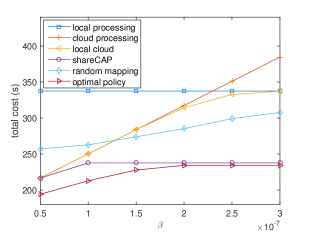
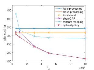
Figure 2: The total system cost versus weight $\beta$ (J/bit).

Figure 3: The total system cost versus CAP CPU rate $f_{A}$ (cycles/s).

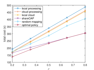
Figure 4: The total system cost versus weight $\rho_{i}=\rho$ (s/J).

Figure 5: The total system cost versus number of users.

In the following, the default parameter values are described, unless otherwise indicated later. We adopt the mobile device characteristics from [49], which is based on a Nokia mobile phone, and set the number of users as $N=8$. According to Tables 1 and 3 in [49], the mobile device has CPU rate $600\times 10^{6}$ cycles/s and processing energy consumption $\frac{1}{650\times 10^{6}}$ J/cycle, and the local computation time $3.95\times 10^{-7}$ s/bit and local processing energy consumption $3.65\times 10^{-7}$ J/bit are calculated when the x264 CBR encode application (1900 cycles/byte) is considered for $Y(i)=1900D_{\mathrm{in}}(i)$. The input and output data sizes of each task are assumed to be uniformly distributed from $10$ to $30$ MB and from $1$ to $3$ MB, respectively.

Both uplink bandwidth $C_{\mathrm{UL}}$ and downlink bandwidth $C_{\mathrm{DL}}$ between mobile users and the CAP are set to $20$ MHz, with no additional limit on the total bandwidth, and the transmission and receiving energy consumptions of the mobile user are both $1.42\times 10^{-7}$ J/bit as indicated in Table 2 in [49]. For simplicity, we set $\eta^{u}_{i}=\eta^{d}_{i}=3.5\ \mathrm{b}/\mathrm{s}/\mathrm{Hz}$ for all $i$. The CPU rates of the CAP and each server at the remote cloud are $3\times 10^{9}$ cycle/s and $2\times 10^{9}$ cycle/s, respectively. When tasks are offloaded to the cloud, the transmission rate $r^{ac}$ is $6$ Mpbs. Also, we set the values of cost $C^{a}_{i}$ and $C^{c}_{i}$ to be the same as that of the input data size $D_{\textrm{in}}(i)$, and $\alpha=1\times 10^{-8}$ J/bit and $\beta=2\times 10^{-7}$ J/bit. We further set $\rho_{i}=\rho=0.5$ s/J for all $i$. Finally, all numerical results are obtained by averaging over 100 realizations of the input and output data sizes of each task.

To study the performance of shareCAP and shareCAP-D, we compare them with the following methods: 1) the local processing only method where all tasks are processed by mobile users, 2) the cloud processing only method where all tasks are offloaded to the cloud, 3) the local-cloud offloading method where the same approximation procedure as the shareCAP method is applied except that there is no CAP, 4) the random mapping method where each task is processed at different locations with equal probability, 5) the optimal policy where the optimal value is obtained by exhaustive search. When compared with shareCAP-D, all of the adaptive adjustment procedure in Section 5 is added to all of the above methods when their offloading decisions are not feasible.

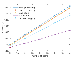
Figure 6: The total system cost versus number of users with scaled resources.

TABLE II: Average run time comparison under various number of users.

Number of	shareCAP (sec)	optimal policy (sec)
users		(exhaustive search)
6	1.65	146.48
7	1.74	445.18
8	1.90	1355.18
9	2.07	4113.86
10	2.22	12539.73
20	4.14	N/A
30	6.56	N/A
40	9.82	N/A
50	14.37	N/A

7.2 Performance of ShareCAP

In Fig. 3, we show the system cost vs. weight $\beta$ on the cloud processing cost. When $\beta$ becomes large, the total system cost puts more emphasis on the cloud usage cost. As a consequence, all tasks are more likely to be processed by either the mobile user or the CAP. The local-cloud method in this case converges to the local processing method. On the other hand, when $\beta$ decreases, the cost of cloud processing becomes insignificant, and shareCAP, local-cloud, and optimal policy all converge to cloud processing.

Though the existence of the CAP can provide additional computation capacity, all tasks processed at the CAP need to share the CAP CPU rate $f_{A}$ by optimally allocating the processing rate to each user’s task. In Fig. 3, we plots the total system cost vs. $f_{A}$. As expected, a more powerful CAP can dramatically increase system performance, and shareCAP converges to local-cloud when the CAP CPU rate is too slow to help.

In Fig. 5, we study the system cost when weight $\rho$ (weight of energy consumption relative to delay) changes. In Figs.  5, and 6, we study the system cost under various number of users $N$. In particular, in Fig. 6, the amount of limited resources (i.e., uplink and downlink bandwidth and the total CAP processing rate) is scaled proportional to the number of users $N$. From Figs. 5 to 6, We observe that with the help of the CAP, shareCAP outperforms all other methods. Furthermore, all of these figures show that, over a wide range of system parameter values, shareCAP provides performance close to that of optimal policy, where the latter, obtained by exhaustive search, has an exponential computational complexity in $N$, i.e., $O(3^{N})$. The corresponding average run times for different values of $N$ are also provided in Table II. They are obtained on a desktop PC with Intel Core i3-4150 3.5 GHz processor and 8 GB RAM. For optimal policy by exhaustive search, we only obtain the run times up to 10 users as the required computational time becomes very high for the cases beyond 10 users.

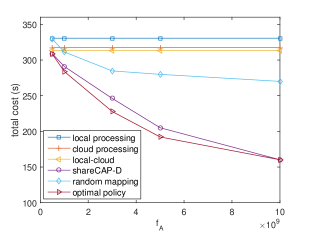
Figure 7: The total system cost versus delay factor $\theta$ with strict delay constraints.

Figure 8: The total system cost versus CAP CPU rate $f_{A}$ (cycles/s) with strict delay constraints.

7.3 Performance of ShareCAP-D

For numerical results with shareCAP-D, we assume $T_{i}\geq\theta T^{l}_{i}$ for all $i$.

Fig. 8 plots the total system cost vs. the delay factor $\theta$. We observe that shareCAP-D provides near-optimal performance unless $\theta$ is close to $1$, i.e., when the problem (53) is nearly infeasible. When $\theta$ is moderately relaxed, there are more offloading decisions can satisfy delay constraints, which allows shareCAP-D to choose a local optimum that is closer to the optimal solution.

In Fig. 8, we plots the total system cost vs. $f_{A}$ with $\theta=1.1$. We see that shareCAP-D outperforms all other methods except the optimal solution. Furthermore, we observe that shareCAP-D is the only method that can efficiently utilize the increasing CAP processing capacity, as demonstrated by it steeply declining cost curve as $f_{A}$ increases. In particular, when $f_{A}\geq 5\times 10^{9}$, shareCAP-D is nearly identical to an optimal policy.

Finally, we plot the total system cost vs. number of users $N$ with $\theta=1.1$ in Fig. 9. Though the optimization problem is more complicated due to additional delay constraints, we see that the system cost of shareCAP-D is still close to that of the optimal policy, showing the scalability of our proposed algorithm for various $N$ values.

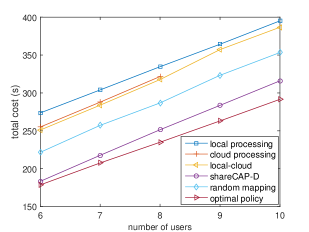
Figure 9: The total system cost versus number of users with strict delay constraints.

8 Conclusion

We have studied a mobile cloud computing system consisting of multiple users, one CAP, and one remote cloud server. We propose a new approach toward joint task offloading and allocation of computation and communication resources, to minimize the weighted total cost of energy, computation, and the maximum delay among all users. Although the optimization problem is non-convex, we propose shareCAP, an efficient heuristic algorithm using SDR and a new randomization mapping approach. For the case with strict delay constraints for each task, we propose shareCAP-D, a three-step algorithm to obtain a feasible solution that is locally optimal. Numerical results suggest that the proposed method gives nearly optimal performance over a wide range of parameter settings, and the resultant efficient utilization of a CAP can bring substantial cost benefit.

References

- [1] M.-H. Chen, M. Dong, and B. Liang, “Joint offloading decision and resource allocation for mobile cloud with computing access point,” in Proc. IEEE International Conference on Acoustics, Speech and Signal Processing (ICASSP), Mar. 2016, pp. 3516–3520.
- [2] K. Kumar, J. Liu, Y.-H. Lu, and B. Bhargava, “A survey of computation offloading for mobile systems,” Mobile Networks and Applications, vol. 18, no. 1, pp. 129–140, Feb. 2013.
- [3] N. Fernando, S. W. Loke, and W. Rahayu, “Mobile cloud computing: A survey,” Future Generation Computer Systems, vol. 29, no. 1, pp. 84 – 106, Jan. 2013.
- [4] H. T. Dinh, C. Lee, D. Niyato, and P. Wang, “A survey of mobile cloud computing: architecture, applications, and approaches,” Wireless Communications and Mobile Computing, vol. 13, no. 18, pp. 1587–1611, 2013.
- [5] ETSI Group Specification, “Mobile edge computing (MEC); framework and reference architecture,” ETSI GS MEC 003 V1.1.1, 2016.
- [6] B. Liang, “Mobile edge computing,” in Key Technologies for 5G Wireless Systems, V. W. S. Wong, R. Schober, D. W. K. Ng, and L.-C. Wang, Eds., Cambridge University Press, 2017.
- [7] T. X. Tran, A. Hajisami, P. Pandey, and D. Pompili, “Collaborative mobile edge computing in 5g networks: New paradigms, scenarios, and challenges,” IEEE Communications Magazine, vol. 55, no. 4, pp. 54–61, Apr. 2017.
- [8] A. Greenberg, J. Hamilton, D. A. Maltz, and P. Patel, “The cost of a cloud: Research problems in data center networks,” ACM SIGCOMM Computer Communication Review, vol. 39, no. 1, pp. 68–73, Dec. 2008.
- [9] M. Satyanarayanan, P. Bahl, R. Caceres, and N. Davies, “The case for VM-based cloudlets in mobile computing,” IEEE Pervasive Computing, vol. 8, no. 4, pp. 14–23, Oct. 2009.
- [10] G. Lewis and P. Lago, “Architectural tactics for cyber-foraging: Results of a systematic literature review,” Journal of Systems and Software, vol. 107, pp. 158 – 186, 2015.
- [11] F. Bonomi, R. Milito, J. Zhu, and S. Addepalli, “Fog computing and its role in the internet of things,” in Proc. ACM SIGCOMM Workshop on Mobile Cloud Computing, Aug. 2012, pp. 13–16.
- [12] S. Boyd and L. Vandenberghe, Convex Optimization. Cambridge University Press, 2004.
- [13] Z.-Q. Luo, W.-K. Ma, A.-C. So, Y. Ye, and S. Zhang, “Semidefinite relaxation of quadratic optimization problems,” IEEE Signal Processing Magazine, vol. 27, no. 3, pp. 20–34, May 2010.
- [14] K. Kumar and Y.-H. Lu, “Cloud computing for mobile users: Can offloading computation save energy?” Computer, vol. 43, no. 4, pp. 51–56, Apr. 2010.
- [15] W. Zhang, Y. Wen, K. Guan, D. Kilper, H. Luo, and D. Wu, “Energy-optimal mobile cloud computing under stochastic wireless channel,” IEEE Transactions on Wireless Communications, vol. 12, no. 9, pp. 4569–4581, Sep. 2013.
- [16] Y. Wen, W. Zhang, and H. Luo, “Energy-optimal mobile application execution: Taming resource-poor mobile devices with cloud clones,” in Proc. IEEE International Conference on Computer Communications (INFOCOM), Mar. 2012, pp. 2716–2720.
- [17] S. Barbarossa, S. Sardellitti, and P. Di Lorenzo, “Computation offloading for mobile cloud computing based on wide cross-layer optimization,” in Proc. Future Network and Mobile Summit (FutureNetworkSummit), Jul. 2013, pp. 1–10.
- [18] O. Munoz, A. Pascual-Iserte, and J. Vidal, “Optimization of radio and computational resources for energy efficiency in latency-constrained application offloading,” IEEE Transactions on Vehicular Technology, vol. 64, no. 10, pp. 4738–4755, Oct. 2015.
- [19] E. Cuervo, A. Balasubramanian, D.-k. Cho, A. Wolman, S. Saroiu, R. Chandra, and P. Bahl, “MAUI: Making smartphones last longer with code offload,” in Proc. ACM International Conference on Mobile Systems, Applications, and Services (MobiSys), Jan. 2010, pp. 49–62.
- [20] B.-G. Chun, S. Ihm, P. Maniatis, M. Naik, and A. Patti, “Clonecloud: Elastic execution between mobile device and cloud,” in Proc. ACM Conference on Computer Systems (EuroSys), Apr. 2011, pp. 301–314.
- [21] S. Kosta, A. Aucinas, P. Hui, R. Mortier, and X. Zhang, “Thinkair: Dynamic resource allocation and parallel execution in the cloud for mobile code offloading,” in Proc. IEEE International Conference on Computer Communications (INFOCOM), Mar. 2012, pp. 945–953.
- [22] Y. Zhang, H. Liu, L. Jiao, and X. Fu, “To offload or not to offload: An efficient code partition algorithm for mobile cloud computing,” in Proc. IEEE International Conference on Cloud Networking (CLOUDNET), Nov. 2012, pp. 80–86.
- [23] W. Zhang, Y. Wen, and D. O. Wu, “Energy-efficient scheduling policy for collaborative execution in mobile cloud computing,” in Proc. IEEE International Conference on Computer Communications (INFOCOM), Apr. 2013, pp. 190–194.
- [24] S. E. Mahmoodi, R. N. Uma, and K. P. Subbalakshmi, “Optimal joint scheduling and cloud offloading for mobile applications,” IEEE Transactions on Cloud Computing, Apr. 2016.
- [25] Y. H. Kao, B. Krishnamachari, M. R. Ra, and F. Bai, “Hermes: Latency optimal task assignment for resource-constrained mobile computing,” in Proc. IEEE International Conference on Computer Communications (INFOCOM), Apr. 2015, pp. 1894–1902.
- [26] H. Wu, W. Knottenbelt, K. Wolter, and Y. Sun, “An optimal offloading partitioning algorithm in mobile cloud computing,” in Proc. International Conference on Quantitative Evaluation of Systems, Aug. 2016, pp. 311–328.
- [27] Y. Zhang, D. Niyato, and P. Wang, “Offloading in mobile cloudlet systems with intermittent connectivity,” IEEE Transactions on Mobile Computing, vol. 14, no. 12, pp. 2516–2529, Dec. 2015.
- [28] T. Truong-Huu, C. K. Tham, and D. Niyato, “To offload or to wait: An opportunistic offloading algorithm for parallel tasks in a mobile cloud,” in Proc. IEEE International Conference on Cloud Computing Technology and Science, Dec. 2014, pp. 182–189.
- [29] D. T. Hoang, D. Niyato, and P. Wang, “Optimal admission control policy for mobile cloud computing hotspot with cloudlet,” in Proc. IEEE Wireless Communications and Networking Conference (WCNC), Apr. 2012, pp. 3145–3149.
- [30] D. T. Hoang, D. Niyato, and L. B. Le, “Simulation-based optimization for admission control of mobile cloudlets,” in Proc. IEEE International Conference on Communications (ICC), Jun. 2014, pp. 3764–3769.
- [31] R. Kaewpuang, D. Niyato, P. Wang, and E. Hossain, “A framework for cooperative resource management in mobile cloud computing,” IEEE Journal on Selected Areas in Communications, vol. 31, no. 12, pp. 2685–2700, Dec. 2013.
- [32] S. Ren and M. van der Schaar, “Efficient resource provisioning and rate selection for stream mining in a community cloud,” IEEE Transactions on Multimedia, vol. 15, no. 4, pp. 723–734, Jun. 2013.
- [33] S. Sardellitti, G. Scutari, and S. Barbarossa, “Joint optimization of radio and computational resources for multicell mobile-edge computing,” IEEE Transactions on Signal and Information Processing over Networks, vol. 1, no. 2, pp. 89–103, Jun. 2015.
- [34] X. Lyu, H. Tian, C. Sengul, and P. Zhang, “Multiuser joint task offloading and resource optimization in proximate clouds,” IEEE Transactions on Vehicular Technology, vol. 66, no. 4, pp. 3435–3447, Apr. 2017.
- [35] X. Chen, “Decentralized computation offloading game for mobile cloud computing,” IEEE Transactions on Parallel and Distributed Systems, vol. 26, no. 4, pp. 974–983, Apr. 2015.
- [36] E. Meskar, T. D. Todd, D. Zhao, and G. Karakostas, “Energy aware offloading for competing users on a shared communication channel,” IEEE Transactions on Mobile Computing, vol. 16, no. 1, pp. 87–96, Jan. 2017.
- [37] X. Chen, L. Jiao, W. Li, and X. Fu, “Efficient multi-user computation offloading for mobile-edge cloud computing,” IEEE/ACM Transactions on Networking, vol. 24, no. 5, pp. 2795–2808, Oct 2016.
- [38] M.-H. Chen, B. Liang, and M. Dong, “Joint offloading decision and resource allocation for multi-user multi-task mobile cloud,” in Proc. IEEE International Conference on Communications (ICC), May 2016.
- [39] H. Viswanathan, P. Pandey, and D. Pompili, “Maestro: Orchestrating concurrent application workflows in mobile device clouds,” in Proc. IEEE International Conference on Autonomic Computing (ICAC), Jul. 2016, pp. 257–262.
- [40] K. Habak, M. Ammar, K. A. Harras, and E. Zegura, “Femto clouds: Leveraging mobile devices to provide cloud service at the edge,” in Proc. IEEE International Conference on Cloud Computing, Jun. 2015, pp. 9–16.
- [41] M. R. Rahimi, N. Venkatasubramanian, S. Mehrotra, and A. V. Vasilakos, “Mapcloud: Mobile applications on an elastic and scalable 2-tier cloud architecture,” in Proc. IEEE/ACM Fifth International Conference on Utility and Cloud Computing, Nov. 2012, pp. 83–90.
- [42] M. R. Rahimi, N. Venkatasubramanian, and A. V. Vasilakos, “Music: Mobility-aware optimal service allocation in mobile cloud computing,” in Proc. IEEE International Conference on Cloud Computing, Jun. 2013, pp. 75–82.
- [43] J. Song, Y. Cui, M. Li, J. Qiu, and R. Buyya, “Energy-traffic tradeoff cooperative offloading for mobile cloud computing,” in Proc. IEEE International Symposium of Quality of Service (IWQoS), May 2014, pp. 284–289.
- [44] V. Cardellini, V. De Nitto Personé, V. Di Valerio, F. Facchinei, V. Grassi, F. Lo Presti, and V. Piccialli, “A game-theoretic approach to computation offloading in mobile cloud computing,” Mathematical Programming, vol. 157, no. 2, pp. 421–449, 2016.
- [45] M.-H. Chen, B. Liang, and M. Dong, “Joint offloading and resource allocation for computation and communication in mobile cloud with computing access point,” in Proc. IEEE International Conference on Computer Communications (INFOCOM), May 2017.
- [46] D. B. Shmoys, J. Wein, and D. P. Williamson, “Scheduling parallel machines on-line,” SIAM J. Comput., vol. 24, no. 6, pp. 1313–1331, Dec. 1995.
- [47] M. Grant, S. Boyd, and Y. Ye, “CVX: Matlab software for disciplined convex programming,” 2009. [Online]. Available: http://cvxr.com/cvx/
- [48] Y. Nesterov, A. Nemirovskii, and Y. Ye, Interior-point polynomial algorithms in convex programming. SIAM, 1994.
- [49] A. P. Miettinen and J. K. Nurminen, “Energy efficiency of mobile clients in cloud computing,” in Proc. USENIX Conference on Hot Topics in Cloud Computing (HotCloud), Jun. 2010, pp. 4–11.