Using the CIFIST grid of CO5BOLD 3D model atmospheres to study the effects of stellar granulation on photometric colours.

Abstract

Context. The atmospheres of cool stars are temporally and spatially inhomogeneous due to the effects of convection. The influence of this inhomogeneity, referred to as granulation, on colours has never been investigated over a large range of effective temperatures and gravities.

Aims. We aim to study, in a quantitative way, the impact of granulation on colours.

Methods. We use the CIFIST (Cosmological Impact of the FIrst Stars) grid of CO⁵BOLD (COnservative COde for the COmputation of COmpressible COnvection in a BOx of L Dimensions, L=2,3) hydrodynamical models to compute emerging fluxes. These in turn are used to compute theoretical colours in the $UBVRI$, 2MASS, Hipparcos, Gaia and SDSS systems. Every CO⁵BOLD model has a corresponding one dimensional (1D) plane-parallel LHD (Lagrangian HydroDynamics) model computed for the same atmospheric parameters, which we used to define a ”3D correction” that can be applied to colours computed from fluxes computed from any 1D model atmosphere code. As an example, we illustrate these corrections applied to colours computed from ATLAS models.

Results. The 3D corrections on colours are generally small, of the order of a few hundredths of a magnitude, yet they are far from negligible. We find that ignoring granulation effects can lead to underestimation of $T\rm_{eff}$ by up to 200 K and overestimation of gravity by up to 0.5 dex, when using colours as diagnostics. We have identified a major shortcoming in how scattering is treated in the current version of the CIFIST grid, which could lead to offsets of the order 0.01 mag, especially for colours involving blue and UV bands. We have investigated the Gaia and Hipparcos photometric systems and found that the $(G-H_{p})$,$(BP-RP)$ diagram is immune to the effects of granulation. In addition, we point to the potential of the RVS photometry as a metallicity diagnostic.

Conclusions. Our investigation shows that the effects of granulation should not be neglected if one wants to use colours as diagnostics of the stellar parameters of F,G,K stars. A limitation is that scattering is treated as true absorption in our current computations, thus our 3D corrections are likely an upper limit to the true effect. We are already computing the next generation of the CIFIST grid, using an approximate treatment of scattering.

1 Introduction

The use of theoretical colours computed from model atmospheres is widespread, however, so far all available grids of theoretical colours (e.g. Bessell et al. 1998; Castelli 1999; Önehag et al. 2009; Casagrande & VandenBerg 2014) are based on one dimensional (1D) static model atmospheres. Extensive computations of fluxes from the three-dimensional (3D) models of the STAGGER grid (Magic et al. 2013) have been done by Magic et al. (2015), however, so-far only the limb-darkening coefficients have been published. In a series of two papers, we wish to explore the parameter space covered by the CIFIST (Cosmological Impact of the FIrst Stars) grid of 3D models (Ludwig et al. 2009, and Ludwig et al., in preparation) that has been computed with the CO⁵BOLD (COnservative COde for the COmputation of COmpressible COnvection in a BOx of L Dimensions, L=2,3) code (Freytag et al. 2012). This effort expands on the pioneering computations of colours from CO⁵BOLD models presented earlier by Kučinskas et al. (2005) and Kučinskas et al. (2009).

For comparison with the CO⁵BOLD models, we computed two grids of 1D model atmospheres. The first was computed using the LHD  (Lagrangian HydroDynamics) 1D model atmosphere code (Caffau & Ludwig 2007) assuming a mixing length parameter $\rm\alpha_{LHD}=1.0$ . The value 1.0 is closest to the value used in the Castelli & Kurucz (2003) grid of ATLAS models; therefore we chose this value here. The effects of different choices of the mixing length parameter in the reference 1D model are further explored in Paper II of the series (Kučinskas et al. 2018). The second grid was computed using ATLAS (Kurucz 2005) assuming a mixing length parameter 1.25, and the Castelli & Kurucz (2003) Opacity Distribution Functions (ODFs) with 2 kms^-1 microturbulence. The choice of mixing length and microturbelent velocity were made to be consistent with the Castelli & Kurucz (2003) grid of ATLAS models. Both grids of models were specifically computed to match atmospheric parameters of the CO⁵BOLD models in the CIFIST grid.

The purpose of the present paper (Paper I of the series) is to present the computational methods employed and compare the fluxes and colours computed from 1D static model atmospheres to those computed from 3D hydrodynamical model atmospheres. We discuss in detail the effects of the treatment of scattering both in the computation of model atmospheres and in the computation of emerging fluxes. For the $UBVRI$, 2MASS, Hipparcos, Gaia and SDSS $ugriz$ systems we provide grids of “3D corrections” that can be applied to colours computed from 1D model atmospheres. We also provide a corresponding grid of ATLAS 3D-corrected colours.

In the second paper of the series (Kučinskas et al. 2018), we select ten model atmospheres for two different metallicities (0.0 and –2.0) that cover the main phases of stellar evolution (main sequence, turn off, sub giant, red giant) and explore the effects of granulation in the corresponding parameter space.

There are some differences of approach to the computation of colours in the two papers, which are explained in detail in Kučinskas et al. (2018). In both papers, we adopt a strictly differential approach, discussing only 3D-1D differences, which makes the above-mentioned differences irrelevant.

2 Computation of synthetic colours

2.1 Photometric systems and zero-points

Table 1: 2MASS in-band fluxes and corresponding magnitudes from Cohen et al. (2003)

Star	$FJ$	$J$	$FH$	$H$	$FK_{S}$	$K_{S}$
	$\rm Wcm^{-2}$	mag	$\rm Wcm^{-2}$	mag	$\rm Wcm^{-2}$	mag
	$\times 10^{-14}$		$\times 10^{-14}$		$\times 10^{-14}$
Vega	15.076	–0.001	12.857	–0.005	1.121	–0.001
0 mag	15.082	–0.000	12.843	–0.000	1.122	–0.000

The problem of computing synthetic colours has been thoroughly addressed in many excellent papers (e.g. Bessell et al. 1998; Castelli 1999; Önehag et al. 2009; Castelli & Kurucz 2006; Bessell & Murphy 2012; Casagrande & VandenBerg 2014). Our own approach to the problem has been extensively described in Bonifacio et al. (2017). We refer the reader to that paper for justification on our choices of zero points for the synthetic photometry and bolometric magnitudes. In this paper, we investigate the $UBVRI$ and Hipparcos-Tycho systems, using the bandpasses defined by Bessell & Murphy (2012), the 2MASS system (Cohen et al. 2003) and the Gaia system, as defined by the pre-launch bandpasses . The above are all “Vega” systems, and we tie the synthetic photometry to Vega using the CALSPEC flux of VEGA and assuming all magnitudes for Vega to be 0.03, except for the 2MASS magnitudes where we assume for Vega J=0.001, H=–0.005 and K=0.001, in order to be consistent with the zero-magnitude fluxes of Cohen et al. (2003, see table 1). As explained in Bonifacio et al. (2017), we did not define the zero points of the “Vega” systems by using a model atmosphere of Vega, since such a model cannot be computed with CO⁵BOLD, but we assumed a radius of $1\,R_{\odot}$ and a distance of 10 pc for each model atmosphere and applied to this flux the same zero points adopted for the observed fluxes. We also investigated the SDSS $ugriz$ system, which is AB type (Oke & Gunn 1983), tied to the standards defined in Fukugita et al. (1996). In the SDSS catalogue, what are reported are not magnitudes, but “luptitudes” defined in Lupton et al. (1999). A “luptitude” is defined as

$$m=-{2.5\over\ln(10)}\left[{\rm asinh}\left((f/f_{0})/(2b)\right)+\ln(b)\right]$$ (1)

where $f$ is the flux of the object ,$f_{0}$ is the flux of the 0 magnitude object, and $b$ is a constant, called the softening parameter. The softening parameter determines the magnitude of an object with zero flux, that is, a non-detection in the survey; this is the magnitude limit of the survey. It is important to keep in mind that objects with magnitudes equal or very close to this limit have essentially undefined colours and therefore should not be compared to theoretical colours. Other SDSS-like systems that are becoming increasingly popular and are used in many telescopes may use magnitudes rather than luptitudes. In order to be able to compare our computed colours directly to the SDSS catalogue, we computed luptitudes rather than magnitudes to derive SDSS colours. We note however that the difference in 3D correction between colours computed using luptitudes and magnitudes is always less than or equal to $10^{-5}$ mag. So for any practical purpose the 3D corrections provided in Tables 14 to 21 can also be applied to any SDSS-like system.

2.2 Computation of emerging fluxes

As described in greater detail in Bonifacio et al. (2017) we used the NLTE3D code to compute the emerging fluxes from the CO⁵BOLD models. Each 3D model is formed by a time series of 3D structures, usually of the order of several hundreds, that we call snapshots. Consecutive snapshots are often correlated, and including correlated events does not improve the statistic. As already mentioned, computations with 3D structures, whether this be fluxes or spectrum synthesis, are time consuming. We then select a representative number of statistically independent snapshots able to represent the model. Usually we select about 20 snapshots from a model, because we think this is a good compromise between the computation time for the fluxes or spectrum synthesis, and the representativeness of the selection for the model. This number has been found to be representative in a detailed investigation on the solar model (Caffau 2009) and we assume this to be the case for any CO⁵BOLD model. The snapshot selection is made so that its statistical properties are the same as those of the total ensemble of computed snapshots; we refer to Caffau & Ludwig (2007) for further details on this. For each model, we averaged the emerging flux from the selected snapshots.

We relied on the Castelli & Kurucz (2003) opacity distribution functions (ODFs) in order to take into account the line opacity. We used the “LITTLE” ODFs, with 1212 frequency points, rather than the “BIG” ODFs that only have 328 frequency points. The continuum opacities were computed using the iondis and opalam routines of the Linfor3D spectrum synthesis code (Steffen et al. 2017; Gallagher et al. 2017).

This approach is inconsistent, since the models have been computed using MARCS continuum and line opacities, while the fluxes have been computed assuming iondis and opalam continuum opacities and ATLAS line opacities. Since we rely mainly on a differential approach (3D-1D), we do not expect this inconsistency to be a major shortcoming, as we explain below.

2.3 The treatment of scattering

Scattering opacity has been treated as true absorption and this, in our view is the main physical limitation of our computation. The treatment of scattering enters on two occasions in our problem: first in the computation of the model, where its treatment may influence the temperature structure of the model, then in the computation of the emerging flux from the model. The choice of treating scattering as true absorption is made for computational reasons. A fully consistent treatment of scattering requires that the mean intensity $J_{\nu}$ be evaluated at each point in the computational box during the computation. Collet et al. (2011) questioned the soundness of treating scattering as true absorption and showed that it may lead to a mean temperature structure that is substantially warmer than that obtained when explicitly treating the scattering. On the other hand, they also noticed that a better and computationally less expensive approximation is to treat scattering as true absorption in the optically thick layers and ignore the scattering opacity in the optically thin layers as described in Hayek et al. (2010). In this approximation one does not really treat scattering while computing the radiative transfer, but uses an appropriate opacity table. Ludwig & Steffen (2012) computed a CO⁵BOLD model using the Hayek et al. (2010) approximation and agreed qualitatively with the conclusions of Collet et al. (2011), although in their case the influence of the treatment of scattering was clearly less important than in the example studied by Collet et al. (2011). In the Ludwig & Steffen (2012) study, the difference in mean temperature between the “true absorption” and “approximate scattering” models is about 100 K at log($\tau$)=–4, while in the Collet et al. (2011) study, this difference is about five times larger. The two models used by Ludwig & Steffen (2012) and Collet et al. (2011) have very similar atmospheric parameters, therefore we attribute this difference between the two studies to differences between the two codes used to compute the hydrodynamical simulations. We have used this model, with $T\rm_{eff}$= 5000 K, log g = 2.5, and metallicity –3.0, and another model, with the same atmospheric parameters, but computed treating scattering as true absorption, to assess the influence of scattering on the computed fluxes and colours. This particular model was chosen because it was in this case that Collet et al. (2011) obtained the largest effects of scattering. Therefore these results may be considered an upper limit to the effects of scattering.

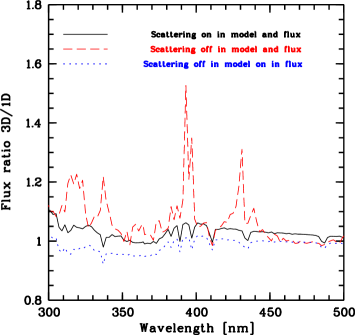
Figure 1: Ratio of the fluxes of one snapshot of the CO⁵BOLD models d3t50g25mm30n01 (scattering treated as true absorption) and d3t50g25mm30n02 (scattering in the Hayek et al. (2010) approximation) to the fluxes computed from their corresponding LHD models under different assumptions. The solid line (black) corresponds to the d3t50g25mm30n02 model, and the flux has been computed fully taking into account scattering. The dashed line (red) corresponds to the d3t50g25mm30n01 model and the flux has been computed treating scattering as true absorption. The dotted line (blue) corresponds again to the d3t50g25mm30n01 model, but in this case scattering has been properly taken into account in the flux computation.

NLTE3D can treat scattering in detail (no approximations) in the computation of the flux from a given model, but the computation is much more intensive. We limited the comparison to a single snapshot. In order to check that a single snapshot is representative, we computed the colours for each of the 20 snapshots that are our selection for this model. The snapshot-to-snapshot difference in colours was always below 0.01 mag. As we shall see below, the differences due to the different assumptions on scattering are always larger than this. Thus our comparison is meaningful.

In Fig. 1, we show the ratio of the flux computed from the CO⁵BOLD models to that of their corresponding LHD models. The dotted line corresponds to the model for which scattering has been treated as true absorption, but scattering has been taken into account in the flux computation. The dashed line corresponds to the same model; however in this case, consistently with what was done for the model computation, also in the flux computation scattering has been treated as true absorption. Finally the solid line corresponds to the model for which scattering has been treated in the approximation of Hayek et al. (2010) and scattering has been fully taken into account in the flux computation. The same approximations apply to both the 1D and 3D models. We present this in the UV-visible region where the differences due to the different treatment of scattering are largest. The first thing that is obvious is that the treatment of scattering mostly affects the spectral regions characterised by strong lines. Treating scattering as true absorption results in a flux from the CO⁵BOLD model that can be 1.2 to almost 1.6 times larger than that in the corresponding LHD model. This is not so in the case where scattering is treated using the Hayek et al. (2010) approximation in the model, and fully treated in the flux computation. In this case, the flux from the CO⁵BOLD model is only about 5% larger than that from the LHD model, but the flux ratio varies rather smoothly with wavelength, unlike what is seen when treating scattering as true absorption. The “hybrid” case, in which we treat scattering in the flux computation using a model which has been computed treating scattering as true absorption, is interesting. In the current version of the CIFIST grid (Ludwig et al. 2009) all models have been computed treating scattering as true absorption. A new version of the grid is currently being computed in which scattering is treated in the Hayek et al. (2010) approximation. In the following, for simplicity, we refer to the case where scattering has been treated as true absorption both in the model and in the flux calculations as “true absorption”; we refer to the case in which the model has been computed treating scattering in the Hayek et al. (2010) approximation and the flux has been computed fully treating scattering as “scattering”; we refer to the case in which the model has been computed treating scattering as true absorption but the flux has been computed fully taking into account scattering, as “hybrid”.

Is there anything to be gained in treating scattering in the flux computation, from the current version of the CIFIST grid? Figure 1 suggests that this is not the case. Although in this hybrid case the run of the 3D/1D ratio has a shape that is very similar to that of the scattering case, it is typically 10% smaller than what is expected in the scattering case. We are ultimately interested in colours and therefore we computed the colour-corrections (3D-1D) for all three cases shown in Fig. 1. Assuming that the scattering computations are the ones closest to the truth we find the difference in 3D correction between the scattering case and the true absorption case is on average –0.013 mag while this difference is –0.009 mag for the hybrid case. Obviously this is largest, in absolute value, for the bluest colours. For $U-B$ we find a difference in the 3D correction of –0.024 for the true absorption case and –0.18 for the hybrid case, while for the $V-K$ colour we find –0.018 for the true absorption case and –0.014 for the hybrid case. In the wavelength range 500 nm to 2500 nm (not shown in Fig. 1) the ratio of the scattering 3D/1D flux ratio to the true absorption 3D/1D flux ratio varies from 0.95 to 1.017 with a mean value of 1.003.

From this test, on one model we decided to use the fluxes computed from the CIFIST grid treating scattering as true absorption. Although the hybrid approach does present a flux that has a similar shape to the consistent scattering approach, we cannot convincingly conclude that this improvement is worth the considerable computational effort needed to perform hybrid computations of the whole grid, considering that the differences in 3D corrections are of only a few thousandths of a magnitude.

All fluxes from the ATLAS models were computed with the ATLAS code, where true absorption was assumed for the continuum scattering and no line scattering was considered. These were also the assumptions adopted in the computation of the ATLAS models.

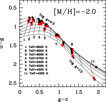
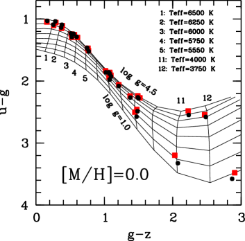
Figure 2: A $u-g$ vs.$g-z$ colour-colour diagram for solar metallicity (bottom panel) and –2.0 (upper panel). The solid lines are the lines of constant temperature and constant surface gravity defined by the Castelli & Kurucz (2003) grid. The black dots correspond to our ATLAS models, that sample points within the Castelli & Kurucz (2003) grid that correspond to the parameters of the models in the CIFIST grid. The Castelli & Kurucz (2003) grid has steps of 250 K in $T\rm_{eff}$ and 0.5 dex in $\log{\rm g}$. The red squares are the “3D-corrected” colours.

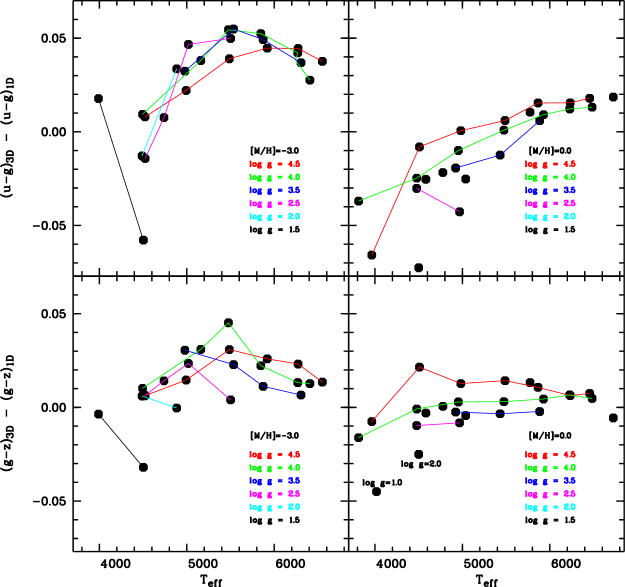
Figure 3: The 3D–1D corrections for the $g-z$ and $u-g$ colours for two metallicities: 0.0 and –3.0.

3 Results

We adopted a differential approach: for each colour, magnitude, or bolometric correction, we computed the “3D correction” as colour (CO⁵BOLD) - colour (LHD). These corrections are provided in the Tables 2 to 21. As an example of how these corrections have to be used, we also provide the ATLAS 3D–corrected colours. For each CO⁵BOLD model we computed an ATLAS model with exactly the same parameters and its emerging flux. From this flux, we computed colours and the 3D corrected colour is then simply colour (ATLAS) + “3D correction”. Clearly, this same procedure can be applied to colours computed from any grid of 1D model atmospheres.

The ATLAS models computed for this paper are almost identical to those of the Castelli & Kurucz (2003) grid. The only difference is that we used updated ODFs for which the contribution of the $\rm H_{2}O$ lines has been revised. This has only a minor effect on models cooler than 4500 K. Our computed colours from our ATLAS models precisely fall on the theoretical curves defined in the Castelli & Kurucz (2003) grid, and may be slightly off for some colours when the temperature decreases due to H₂O opacity.

Figure 2 depicts colour-colour diagrams for $g-z$ and $u-g$ bands for metallicities at [M/H]=0.0 and –2.0. If the metallicity is known (e.g. for stars in a cluster) such a diagram can be used as a diagnostic in $T\rm_{eff}$ and $\log{\rm g}$. While the corrections are generally small around the solar chemical composition, they increase with decreasing metallicity. At low metallicity, the 3D-corrected $g-z$ tends to be larger (i.e. redder), therefore, hotter temperatures will be found from observed g-z colours. At the hot end of our model grid, this change is rather large, of the order of 200 K. At solar metallicity the situation is similar for the hotter models, however for the cooler models ($T\rm_{eff}$$<4500$ K) the situation reverses and the 3D-corrected $g-z$ is smaller (bluer); thus, for a given observed $g-z,$ one would infer a cooler $T\rm_{eff}$, although by only about 50 K. A similar behaviour is observed for the $u-g$ colour at low metallicity; the 3D-corrected $u-g$ is larger, thus, for an observed $u-g,$ one infers a lower gravity, by almost 0.5  dex. At solar metallicity the situation is different. For the hotter models, there is hardly any change in $u-g$, but below 5500 K the 3D-corrected $u-g$ is smaller, implying gravities that are larger, by about 0.1 dex. The situation is illustrated in Fig.3, where the 3D-1D corrections for metallicities 0.0 and –3.0 are plotted as a function of $T\rm_{eff}$. To guide the eye, the corrections relative to models with the same surface gravity are connected by a solid line and a different colour is used for each surface gravity as given in the legend.

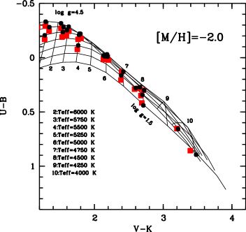
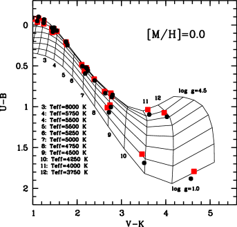
Figure 4: A $U-B$ vs. $V-K$ colour-colour diagram for solar metallicity (bottom panel) and –2.0 (upper panel). The meaning of the lines and symbols is the same as in Fig. 2.

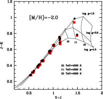
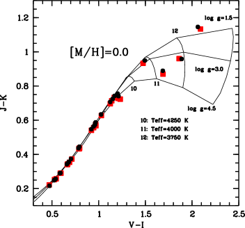
Figure 5: A $J-K$ vs. $V-I$ colour-colour diagram for solar metallicity (bottom panel) and –2.0 (upper panel). The meaning of the lines and symbols is the same as in Fig. 2.

In Fig. 4 we show the $U-B$ versus $V-K$ diagram, which is morphologically similar to the $u-g$ versus $g-z$, and thus the effect of granulation is similar. However, the use of the longer baseline colour $V-K$ makes another effect apparent. At all metallicities, the 3D-corrected colours are redder for the hotter models and bluer for the cooler models. This results in a more compressed scale in $V-K$. It is also apparent that the difference in inferred temperature is smaller in this case, less than 100 K for all gravities and metallicities.

In Fig. 5 we compare two colours that are often used as temperature indicators: $V-I$ and $J-K$. There is a tight correlation between the two colours, up to about 4250 K when the relation splits up and the two colours respond differently to changes in gravity. The “3D-corrected” colours show exactly the same behaviour, except that the relation is offset by 0.05 mag.

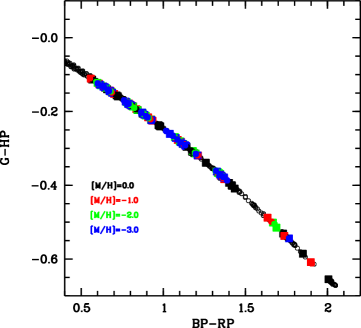
Figure 6: The colour G$-H_{p}$ as a function of the BP–RP colour. Colours computed from models of different metallicity are shown with a different colour: black for [M/H]=0.0, red for [M/H]=–1.0, green for [M/H]=–2.0 and blue for [M/H]=–3.0. Open circles are the colours computed from ATLAS models, while filled squares are the corresponding 3D-corrected colours. We stress that the Gaia bands are the pre-launch bands.

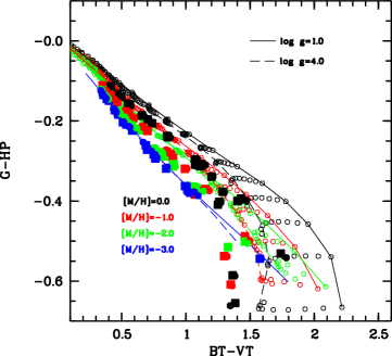
Figure 7: The colour G$-H_{p}$ as a function of the BT–VT colour. Symbols are the same as in Fig. 6. The dashed lines connect the points from the Castelli & Kurucz (2003) grid.

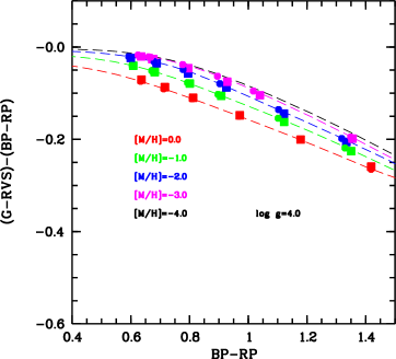
Figure 8: The $CaT$ colour as a function of the $BP-RP$ colour for models with log g=4.0. Filled circles are the colours from the ATLAS models and filled squares are the 3D-corrected colours.

Let us turn our attention to the Gaia photometry. We should warn the reader that the Gaia colours have been computed using the pre-launch transmission curves. This is useful to gain an understanding of the general properties of this photometry. Detailed comparison with the observations will be possible when the post-launch transmission curves become available, after the Gaia Data Release 2. We notice that the wide band used for the Gaia photometry, G, is sufficiently different from the analogue band of Hipparcos, $H_{p}$, that the colour G$-H_{p}$ is tightly correlated with effective temperature. Even more interestingly, it is very tightly correlated with the colour that can be formed from the Blue Prism (BP) and Red Prism (RP) spectra, BP–RP. In Fig. 6 we show how this colour-colour diagram provides a very tight correlation, essentially putting all the stars of any metallicity or gravity on the same relation. It is interesting to note that the 3D corrections do not destroy this correlation, since all the points move along the curve. This should be a very robust correlation and should prove useful to determine the effective pass-bands of the Gaia system and reddening and to detect binary systems. Any star that is an outlier with respect to such a correlation should be considered as a potential binary system. The G$-H_{p}$ correlates with any temperature-dependent colour, in particular with any colour that measures the slope of the Paschen continuum. With other colours, however, the relation splits due to gravity and metallicity dependencies. As an example, we show its correlation with the Tycho $B_{T}-V_{T}$ colour in Fig. 7. In this case the 3D corrections induce relations that are distinctly different from what is deduced from the 1D model atmospheres. Because of the splitting seen due to surface gravity and metallicity, such a colour-colour diagram has a clear diagnostic potential, however the theoretical colours must be properly modelled.

Finally let us turn our attention to the potential of the RVS colour as a metallicity diagnostic. At the faint end of the sensitivity of the RVS spectrograph (Katz et al. 2004), in the interval G=15 to G=17, it is likely that the spectra will be too noisy to allow a metallicity determination. Yet, since the spectra will be flux-calibrated one can derive an RVS magnitude, that is, a narrow-band filter centered on the IR Ca ii triplet. In ground-based observations, such a filter is not very useful, since the signal of the Ca ii lines is severely diluted by the signal coming from the atmospheric OH emission lines. Data taken from space, however, like Gaia, do not suffer from such a limitation. In Fig. 8 we show the behaviour of the $CaT$ colour as a function of the $BP-RP$ colour. We show several metallicities for log g=4.0 and it is clear that even a precision of 0.02 mag in this colour should allow an estimate of the metallicity with a precision of 0.5  dex, down to a metallicity of –3.0, at least. The colour is not strongly sensitive to gravity. However Gaia will also provide the parallaxes, thus the surface gravity will be known. It is interesting to see that the 3D corrections move the points along the curve defined by the 1D models, so that the metallicity sensitivity of the colour remains the same. The metallicity information from the RVS magnitude will be complementary to that coming from the full spectral energy distribution, derived from the prism spectra, for stars for which both will be available.

4 Conclusions

We have used the CIFIST grid of CO⁵BOLD models to investigate the effects of granulation on fluxes and colours of stars of spectral type F, G, and K. Our investigation is exploratory, since we realise that treating scattering as true absorption, as done in the current version of the CIFIST models, leads to incorrect results in the computed emerging fluxes, especially in the blue and UV regions. The influence of this assumption can be quantified in terms of colours and is of the order of 0.02 magnitudes for colours involving blue or UV bands. While the next generation of the CIFIST grid is being computed using the approximate treatment of scattering suggested by Hayek et al. (2010), we believe it is still interesting to publish the results obtained from the current version of the CIFIST grid.

The effects of granulation on colours are generally small, of a few hundredths of a magnitude; they cannot, however be considered negligible. On some colours, such as $g-z,$ the effect can translate to a temperature estimate that is hotter by 200 K.

We publish tables with 3D corrections that can be applied to colours computed from any 1D model atmosphere. For $T\rm_{eff}$$\geq 5000$K, the corrections are smooth enough, as a function of atmospheric parameters, that it is possible to interpolate the corrections between grid points; thus the coarseness of the CIFIST grid should not be a major limitation. However at the cool end there are still far too few models to allow a reliable interpolation.

We have investigated the effects on the Gaia photometric system, although only the pre-launch transmission curves are available. We confirm that a tight correlation between the G$-H_{p}$ colour and the BP–RP colour should exist, and that this correlation should be the same also after granulation effects are taken into account. We have also investigated the potential of the (G–RVS)–(BP–RP) colour as a metallicity diagnostic and we confirm that it is indeed a good indicator, even after 3D corrections have been taken into account, provided this colour can be measured with a precision of 0.02 mag or better. If one is only interested in selecting stars that are more metal-poor than –3.0, the colour is still very powerful even if the precision is of the order of 0.05  mag.

Appendix A Tables of colours and colour corrections.

In this Appendix we present the 3D-1D colour corrections for colours in the Johnson-Cousins, 2MASS, Hipparcos, Gaia and SDSS systems. Bolometric corrections are also provided for the Gaia $G$ magnitude. For each colour, we provide the colour from the ATLAS model, and the “3D-corrected” colour, that is, the ATLAS colour to which we added the corresponding 3D-1D corrections. The 3D-corrected colours can be used directly to interpret observed colours. The 3D corrections can also be used to correct colours computed from any 1D model atmosphere.

Table 2: Colours and corrections for the Johnson-Cousins system for metallicity [M/H]=0.0. In columns labelled ‘ATLAS_c’ the 3D correction has been added to the ATLAS colour.

$T\rm_{eff}$	log g	$U-B$	$U-B$	$\Delta_{U-B}$	$B-V$	$B-V$	$\Delta_{B-V}$	$V-R$	$V-R$	$\Delta_{V-R}$	$V-I$	$V-I$	$\Delta_{V-I}$
		ATLAS	ATLASc	3D-1D	ATLAS	ATLASc	3D-1D	ATLAS	ATLASc	3D-1D	ATLAS	ATLASc	3D-1D
3635	1.00	$+1.880$	$+1.792$	$-0.089$	$+1.671$	$+1.583$	$-0.014$	$+0.944$	$+0.956$	$+0.012$	$+2.062$	$+2.090$	$+0.028$
3813	4.00	$+1.123$	$+1.073$	$-0.050$	$+1.306$	$+1.256$	$+0.032$	$+0.878$	$+0.872$	$-0.006$	$+1.888$	$+1.861$	$-0.027$
4018	1.50	$+1.688$	$+1.580$	$-0.108$	$+1.541$	$+1.433$	$-0.034$	$+0.783$	$+0.764$	$-0.019$	$+1.495$	$+1.476$	$-0.019$
3964	4.50	$+1.095$	$+1.035$	$-0.060$	$+1.314$	$+1.255$	$-0.015$	$+0.844$	$+0.832$	$-0.012$	$+1.687$	$+1.689$	$+0.002$
4501	2.00	$+1.069$	$+1.011$	$-0.058$	$+1.268$	$+1.210$	$-0.027$	$+0.608$	$+0.601$	$-0.007$	$+1.149$	$+1.140$	$-0.009$
4477	2.50	$+1.004$	$+0.979$	$-0.025$	$+1.235$	$+1.210$	$-0.012$	$+0.618$	$+0.615$	$-0.003$	$+1.169$	$+1.167$	$-0.003$
4478	4.00	$+0.854$	$+0.833$	$-0.021$	$+1.136$	$+1.115$	$-0.008$	$+0.645$	$+0.640$	$-0.005$	$+1.203$	$+1.207$	$+0.005$
4509	4.50	$+0.879$	$+0.874$	$-0.005$	$+1.127$	$+1.122$	$-0.003$	$+0.658$	$+0.659$	$+0.001$	$+1.212$	$+1.231$	$+0.019$
4582	3.20	$+0.834$	$+0.813$	$-0.021$	$+1.143$	$+1.122$	$-0.008$	$+0.595$	$+0.593$	$-0.002$	$+1.123$	$+1.124$	$+0.001$
4777	3.20	$+0.679$	$+0.662$	$-0.017$	$+1.067$	$+1.049$	$-0.008$	$+0.540$	$+0.540$	$+0.000$	$+1.026$	$+1.029$	$+0.003$
4968	2.50	$+0.594$	$+0.561$	$-0.033$	$+1.019$	$+0.986$	$-0.020$	$+0.496$	$+0.494$	$-0.002$	$+0.945$	$+0.946$	$+0.001$
5038	3.00	$+0.503$	$+0.485$	$-0.019$	$+0.969$	$+0.950$	$-0.014$	$+0.481$	$+0.481$	$-0.001$	$+0.921$	$+0.922$	$+0.001$
4923	3.50	$+0.558$	$+0.543$	$-0.014$	$+0.998$	$+0.983$	$-0.009$	$+0.508$	$+0.507$	$-0.000$	$+0.967$	$+0.969$	$+0.002$
4954	4.00	$+0.529$	$+0.522$	$-0.007$	$+0.971$	$+0.965$	$-0.004$	$+0.507$	$+0.509$	$+0.002$	$+0.962$	$+0.966$	$+0.004$
4982	4.50	$+0.520$	$+0.523$	$+0.003$	$+0.951$	$+0.954$	$+0.001$	$+0.510$	$+0.516$	$+0.006$	$+0.961$	$+0.970$	$+0.010$
5432	3.50	$+0.247$	$+0.239$	$-0.008$	$+0.798$	$+0.790$	$-0.012$	$+0.411$	$+0.410$	$-0.001$	$+0.794$	$+0.795$	$+0.001$
5475	4.00	$+0.209$	$+0.212$	$+0.003$	$+0.781$	$+0.784$	$-0.005$	$+0.407$	$+0.408$	$+0.001$	$+0.784$	$+0.788$	$+0.004$
5488	4.50	$+0.202$	$+0.207$	$+0.006$	$+0.779$	$+0.784$	$+0.003$	$+0.409$	$+0.414$	$+0.005$	$+0.784$	$+0.794$	$+0.010$
5774	4.40	$+0.068$	$+0.077$	$+0.009$	$+0.680$	$+0.689$	$+0.003$	$+0.364$	$+0.368$	$+0.004$	$+0.703$	$+0.712$	$+0.009$
5884	3.50	$+0.082$	$+0.091$	$+0.009$	$+0.632$	$+0.641$	$-0.012$	$+0.342$	$+0.341$	$-0.001$	$+0.665$	$+0.667$	$+0.002$
5928	4.00	$+0.034$	$+0.043$	$+0.010$	$+0.624$	$+0.633$	$-0.004$	$+0.339$	$+0.340$	$+0.001$	$+0.659$	$+0.664$	$+0.005$
5865	4.50	$+0.031$	$+0.045$	$+0.014$	$+0.652$	$+0.666$	$+0.003$	$+0.352$	$+0.355$	$+0.004$	$+0.681$	$+0.688$	$+0.007$
6228	4.00	$-0.027$	$-0.015$	$+0.012$	$+0.531$	$+0.543$	$-0.003$	$+0.299$	$+0.300$	$+0.001$	$+0.584$	$+0.590$	$+0.006$
6233	4.50	$-0.069$	$-0.054$	$+0.014$	$+0.541$	$+0.555$	$-0.000$	$+0.303$	$+0.305$	$+0.002$	$+0.591$	$+0.595$	$+0.005$
6484	4.00	$-0.049$	$-0.036$	$+0.013$	$+0.461$	$+0.474$	$-0.003$	$+0.267$	$+0.267$	$+0.000$	$+0.522$	$+0.526$	$+0.004$
6456	4.50	$-0.101$	$-0.085$	$+0.016$	$+0.481$	$+0.497$	$+0.001$	$+0.276$	$+0.278$	$+0.002$	$+0.539$	$+0.544$	$+0.005$
6726	4.30	$-0.091$	$-0.073$	$+0.018$	$+0.411$	$+0.429$	$-0.004$	$+0.242$	$+0.239$	$-0.003$	$+0.473$	$+0.470$	$-0.003$

Table 3: Colours and corrections for the Johnson-Cousins system for metallicity [M/H]=–1.0. In columns labelled ‘ATLAS_c’ the 3D correction has been added to the ATLAS colour.

$T\rm_{eff}$	log g	$U-B$	$U-B$	$\Delta_{U-B}$	$B-V$	$B-V$	$\Delta_{B-V}$	$V-R$	$V-R$	$\Delta_{V-R}$	$V-I$	$V-I$	$\Delta_{V-I}$
		ATLAS	ATLASc	3D-1D	ATLAS	ATLASc	3D-1D	ATLAS	ATLASc	3D-1D	ATLAS	ATLASc	3D-1D
3790	4.00	$+0.882$	$+0.843$	$-0.038$	$+1.326$	$+1.288$	$-0.012$	$+0.873$	$+0.859$	$-0.013$	$+1.744$	$+1.739$	$-0.005$
4040	1.50	$+1.068$	$+0.996$	$-0.073$	$+1.339$	$+1.266$	$-0.031$	$+0.736$	$+0.718$	$-0.018$	$+1.424$	$+1.403$	$-0.021$
4001	4.50	$+0.800$	$+0.768$	$-0.032$	$+1.268$	$+1.236$	$-0.020$	$+0.818$	$+0.806$	$-0.012$	$+1.555$	$+1.560$	$+0.006$
4485	2.00	$+0.553$	$+0.526$	$-0.027$	$+1.069$	$+1.042$	$-0.021$	$+0.575$	$+0.571$	$-0.004$	$+1.137$	$+1.132$	$-0.005$
4490	2.50	$+0.484$	$+0.479$	$-0.004$	$+1.036$	$+1.031$	$-0.005$	$+0.576$	$+0.577$	$+0.001$	$+1.136$	$+1.139$	$+0.003$
4525	4.00	$+0.417$	$+0.440$	$+0.023$	$+0.978$	$+1.000$	$+0.014$	$+0.595$	$+0.609$	$+0.013$	$+1.145$	$+1.167$	$+0.022$
4499	4.50	$+0.469$	$+0.471$	$+0.003$	$+0.994$	$+0.997$	$+0.003$	$+0.624$	$+0.628$	$+0.004$	$+1.180$	$+1.193$	$+0.013$
4754	2.50	$+0.309$	$+0.307$	$-0.002$	$+0.927$	$+0.925$	$-0.010$	$+0.507$	$+0.509$	$+0.002$	$+1.013$	$+1.016$	$+0.004$
4993	2.50	$+0.179$	$+0.191$	$+0.011$	$+0.830$	$+0.842$	$-0.008$	$+0.459$	$+0.462$	$+0.003$	$+0.921$	$+0.928$	$+0.007$
4930	3.50	$+0.156$	$+0.170$	$+0.014$	$+0.836$	$+0.850$	$+0.003$	$+0.475$	$+0.482$	$+0.008$	$+0.947$	$+0.958$	$+0.011$
4986	4.00	$+0.127$	$+0.154$	$+0.027$	$+0.814$	$+0.841$	$+0.013$	$+0.469$	$+0.483$	$+0.014$	$+0.931$	$+0.950$	$+0.019$
5061	4.50	$+0.102$	$+0.125$	$+0.022$	$+0.790$	$+0.812$	$+0.008$	$+0.460$	$+0.472$	$+0.012$	$+0.910$	$+0.923$	$+0.014$
5481	3.50	$-0.067$	$-0.035$	$+0.032$	$+0.649$	$+0.680$	$+0.006$	$+0.381$	$+0.389$	$+0.008$	$+0.770$	$+0.784$	$+0.014$
5532	4.00	$-0.103$	$-0.075$	$+0.027$	$+0.639$	$+0.666$	$+0.004$	$+0.376$	$+0.383$	$+0.007$	$+0.759$	$+0.769$	$+0.010$
5473	4.50	$-0.087$	$-0.059$	$+0.027$	$+0.665$	$+0.692$	$+0.006$	$+0.388$	$+0.397$	$+0.009$	$+0.779$	$+0.791$	$+0.012$
5772	4.40	$-0.176$	$-0.150$	$+0.026$	$+0.576$	$+0.602$	$+0.006$	$+0.346$	$+0.354$	$+0.008$	$+0.700$	$+0.712$	$+0.012$
5890	3.50	$-0.133$	$-0.092$	$+0.041$	$+0.523$	$+0.564$	$+0.007$	$+0.325$	$+0.332$	$+0.007$	$+0.661$	$+0.676$	$+0.015$
5850	4.00	$-0.171$	$-0.137$	$+0.034$	$+0.545$	$+0.579$	$+0.003$	$+0.334$	$+0.338$	$+0.004$	$+0.677$	$+0.684$	$+0.007$
5923	4.50	$-0.210$	$-0.171$	$+0.039$	$+0.537$	$+0.576$	$+0.013$	$+0.328$	$+0.338$	$+0.009$	$+0.665$	$+0.679$	$+0.014$
6210	3.50	$-0.135$	$-0.102$	$+0.033$	$+0.441$	$+0.474$	$-0.005$	$+0.284$	$+0.284$	$-0.000$	$+0.581$	$+0.583$	$+0.001$
6261	4.00	$-0.196$	$-0.158$	$+0.038$	$+0.447$	$+0.485$	$+0.003$	$+0.286$	$+0.287$	$+0.001$	$+0.585$	$+0.587$	$+0.001$
6236	4.00	$-0.196$	$-0.165$	$+0.030$	$+0.442$	$+0.472$	$+0.004$	$+0.284$	$+0.288$	$+0.004$	$+0.579$	$+0.588$	$+0.009$
6238	4.50	$-0.247$	$-0.209$	$+0.037$	$+0.460$	$+0.497$	$+0.011$	$+0.291$	$+0.298$	$+0.006$	$+0.594$	$+0.604$	$+0.010$
6503	4.00	$-0.184$	$-0.153$	$+0.031$	$+0.392$	$+0.423$	$+0.002$	$+0.255$	$+0.256$	$+0.001$	$+0.524$	$+0.526$	$+0.003$
6456	4.50	$-0.251$	$-0.211$	$+0.039$	$+0.414$	$+0.454$	$+0.013$	$+0.267$	$+0.274$	$+0.007$	$+0.546$	$+0.558$	$+0.012$
6730	4.30	$-0.208$	$-0.189$	$+0.019$	$+0.359$	$+0.378$	$+0.003$	$+0.234$	$+0.236$	$+0.001$	$+0.481$	$+0.485$	$+0.004$

Table 4: Colours and corrections for the Johnson-Cousins system for metallicity [M/H]=–2.0. In columns labelled ‘ATLAS_c’ the 3D correction has been added to the ATLAS colour.

$T\rm_{eff}$	log g	$U-B$	$U-B$	$\Delta_{U-B}$	$B-V$	$B-V$	$\Delta_{B-V}$	$V-R$	$V-R$	$\Delta_{V-R}$	$V-I$	$V-I$	$\Delta_{V-I}$
		ATLAS	ATLASc	3D-1D	ATLAS	ATLASc	3D-1D	ATLAS	ATLASc	3D-1D	ATLAS	ATLASc	3D-1D
4001	1.50	$+0.895$	$+0.857$	$-0.038$	$+1.336$	$+1.298$	$-0.015$	$+0.733$	$+0.729$	$-0.004$	$+1.440$	$+1.433$	$-0.007$
4000	4.50	$+0.657$	$+0.654$	$-0.003$	$+1.255$	$+1.252$	$-0.001$	$+0.785$	$+0.784$	$-0.001$	$+1.490$	$+1.491$	$+0.000$
4506	1.50	$+0.440$	$+0.417$	$-0.023$	$+1.050$	$+1.027$	$-0.039$	$+0.568$	$+0.563$	$-0.004$	$+1.143$	$+1.139$	$-0.004$
4506	2.00	$+0.301$	$+0.300$	$-0.000$	$+0.989$	$+0.988$	$-0.011$	$+0.557$	$+0.564$	$+0.007$	$+1.126$	$+1.138$	$+0.013$
4478	2.50	$+0.344$	$+0.350$	$+0.006$	$+1.006$	$+1.012$	$+0.001$	$+0.555$	$+0.565$	$+0.010$	$+1.123$	$+1.136$	$+0.013$
4504	4.00	$+0.272$	$+0.283$	$+0.011$	$+0.960$	$+0.971$	$+0.015$	$+0.571$	$+0.582$	$+0.011$	$+1.133$	$+1.147$	$+0.015$
4539	4.50	$+0.280$	$+0.290$	$+0.010$	$+0.959$	$+0.969$	$+0.012$	$+0.576$	$+0.584$	$+0.008$	$+1.134$	$+1.146$	$+0.012$
4743	2.50	$+0.129$	$+0.132$	$+0.004$	$+0.871$	$+0.875$	$-0.014$	$+0.497$	$+0.501$	$+0.005$	$+1.013$	$+1.020$	$+0.006$
4778	2.00	$+0.164$	$+0.206$	$+0.042$	$+0.872$	$+0.914$	$-0.014$	$+0.495$	$+0.490$	$-0.005$	$+1.008$	$+0.998$	$-0.010$
5024	2.50	$-0.012$	$+0.017$	$+0.029$	$+0.745$	$+0.774$	$-0.012$	$+0.444$	$+0.448$	$+0.004$	$+0.912$	$+0.919$	$+0.007$
4976	3.50	$-0.030$	$-0.005$	$+0.026$	$+0.772$	$+0.798$	$+0.004$	$+0.454$	$+0.465$	$+0.012$	$+0.928$	$+0.943$	$+0.015$
4955	4.00	$-0.010$	$+0.022$	$+0.031$	$+0.789$	$+0.820$	$+0.010$	$+0.462$	$+0.477$	$+0.015$	$+0.940$	$+0.959$	$+0.019$
5013	4.50	$-0.019$	$+0.006$	$+0.025$	$+0.778$	$+0.803$	$+0.007$	$+0.458$	$+0.470$	$+0.012$	$+0.927$	$+0.941$	$+0.014$
5502	2.50	$-0.112$	$-0.076$	$+0.036$	$+0.563$	$+0.599$	$-0.014$	$+0.367$	$+0.366$	$-0.000$	$+0.760$	$+0.763$	$+0.002$
5505	3.50	$-0.209$	$-0.168$	$+0.041$	$+0.579$	$+0.620$	$+0.005$	$+0.371$	$+0.377$	$+0.006$	$+0.769$	$+0.777$	$+0.008$
5472	4.00	$-0.220$	$-0.177$	$+0.042$	$+0.604$	$+0.646$	$+0.016$	$+0.379$	$+0.392$	$+0.013$	$+0.782$	$+0.801$	$+0.019$
5479	4.50	$-0.221$	$-0.181$	$+0.040$	$+0.618$	$+0.658$	$+0.012$	$+0.383$	$+0.394$	$+0.012$	$+0.786$	$+0.800$	$+0.014$
5772	3.70	$-0.253$	$-0.201$	$+0.052$	$+0.509$	$+0.561$	$+0.015$	$+0.337$	$+0.345$	$+0.008$	$+0.701$	$+0.712$	$+0.012$
5734	4.40	$-0.285$	$-0.244$	$+0.041$	$+0.539$	$+0.580$	$+0.018$	$+0.347$	$+0.357$	$+0.010$	$+0.718$	$+0.732$	$+0.014$
5861	3.50	$-0.236$	$-0.189$	$+0.047$	$+0.482$	$+0.530$	$+0.007$	$+0.324$	$+0.329$	$+0.004$	$+0.675$	$+0.682$	$+0.007$
5856	4.00	$-0.282$	$-0.233$	$+0.049$	$+0.496$	$+0.544$	$+0.016$	$+0.329$	$+0.337$	$+0.008$	$+0.683$	$+0.695$	$+0.012$
5923	4.50	$-0.316$	$-0.269$	$+0.047$	$+0.494$	$+0.541$	$+0.021$	$+0.325$	$+0.335$	$+0.011$	$+0.674$	$+0.688$	$+0.015$
6287	3.50	$-0.206$	$-0.168$	$+0.038$	$+0.392$	$+0.430$	$+0.002$	$+0.271$	$+0.274$	$+0.002$	$+0.569$	$+0.574$	$+0.005$
6206	4.00	$-0.281$	$-0.246$	$+0.036$	$+0.421$	$+0.457$	$+0.008$	$+0.287$	$+0.290$	$+0.003$	$+0.600$	$+0.606$	$+0.006$
6323	4.50	$-0.331$	$-0.290$	$+0.042$	$+0.412$	$+0.453$	$+0.017$	$+0.279$	$+0.287$	$+0.007$	$+0.583$	$+0.594$	$+0.011$
6534	4.00	$-0.249$	$-0.215$	$+0.034$	$+0.362$	$+0.396$	$+0.006$	$+0.250$	$+0.252$	$+0.003$	$+0.525$	$+0.529$	$+0.005$
6533	4.50	$-0.319$	$-0.281$	$+0.038$	$+0.376$	$+0.415$	$+0.015$	$+0.257$	$+0.263$	$+0.006$	$+0.538$	$+0.547$	$+0.009$

Table 5: Colours and corrections for the Johnson-Cousins system for metallicity [M/H]=–3.0. In columns labelled ‘ATLAS_c’ the 3D correction has been added to the ATLAS colour.

$T\rm_{eff}$	log g	$U-B$	$U-B$	$\Delta_{U-B}$	$B-V$	$B-V$	$\Delta_{B-V}$	$V-R$	$V-R$	$\Delta_{V-R}$	$V-I$	$V-I$	$\Delta_{V-I}$
		ATLAS	ATLASc	3D-1D	ATLAS	ATLASc	3D-1D	ATLAS	ATLASc	3D-1D	ATLAS	ATLASc	3D-1D
3990	1.50	$+0.962$	$+0.980$	$+0.018$	$+1.437$	$+1.456$	$-0.010$	$+0.769$	$+0.771$	$+0.002$	$+1.515$	$+1.518$	$+0.003$
4503	1.50	$+0.373$	$+0.338$	$-0.035$	$+1.039$	$+1.004$	$-0.050$	$+0.583$	$+0.576$	$-0.006$	$+1.177$	$+1.171$	$-0.007$
4488	2.00	$+0.302$	$+0.298$	$-0.005$	$+1.011$	$+1.006$	$-0.016$	$+0.571$	$+0.577$	$+0.006$	$+1.159$	$+1.170$	$+0.011$
4523	2.50	$+0.214$	$+0.207$	$-0.006$	$+0.965$	$+0.958$	$-0.012$	$+0.553$	$+0.560$	$+0.007$	$+1.126$	$+1.136$	$+0.011$
4494	4.00	$+0.193$	$+0.201$	$+0.008$	$+0.973$	$+0.981$	$+0.005$	$+0.572$	$+0.578$	$+0.005$	$+1.157$	$+1.164$	$+0.007$
4522	4.50	$+0.186$	$+0.193$	$+0.007$	$+0.967$	$+0.974$	$+0.003$	$+0.571$	$+0.575$	$+0.004$	$+1.152$	$+1.156$	$+0.004$
4739	2.50	$+0.049$	$+0.060$	$+0.010$	$+0.837$	$+0.848$	$-0.007$	$+0.500$	$+0.508$	$+0.008$	$+1.027$	$+1.042$	$+0.015$
4891	1.80	$+0.049$	$+0.067$	$+0.018$	$+0.769$	$+0.787$	$-0.010$	$+0.473$	$+0.478$	$+0.005$	$+0.975$	$+0.985$	$+0.010$
4884	2.00	$+0.023$	$+0.055$	$+0.033$	$+0.767$	$+0.800$	$-0.010$	$+0.473$	$+0.475$	$+0.003$	$+0.974$	$+0.979$	$+0.005$
5018	2.50	$-0.089$	$-0.049$	$+0.041$	$+0.698$	$+0.739$	$+0.005$	$+0.443$	$+0.453$	$+0.010$	$+0.919$	$+0.937$	$+0.018$
4978	3.50	$-0.113$	$-0.087$	$+0.026$	$+0.734$	$+0.760$	$+0.013$	$+0.455$	$+0.467$	$+0.013$	$+0.938$	$+0.959$	$+0.020$
5160	4.00	$-0.186$	$-0.157$	$+0.030$	$+0.676$	$+0.706$	$+0.018$	$+0.427$	$+0.439$	$+0.012$	$+0.883$	$+0.902$	$+0.019$
4992	4.50	$-0.102$	$-0.083$	$+0.019$	$+0.759$	$+0.778$	$+0.007$	$+0.466$	$+0.473$	$+0.007$	$+0.954$	$+0.964$	$+0.010$
5501	2.50	$-0.167$	$-0.120$	$+0.047$	$+0.536$	$+0.583$	$-0.007$	$+0.363$	$+0.366$	$+0.003$	$+0.762$	$+0.769$	$+0.007$
5535	3.50	$-0.272$	$-0.227$	$+0.045$	$+0.542$	$+0.588$	$+0.015$	$+0.365$	$+0.374$	$+0.009$	$+0.764$	$+0.778$	$+0.014$
5476	4.00	$-0.282$	$-0.241$	$+0.041$	$+0.572$	$+0.613$	$+0.028$	$+0.377$	$+0.393$	$+0.016$	$+0.786$	$+0.813$	$+0.027$
5487	4.50	$-0.285$	$-0.256$	$+0.029$	$+0.586$	$+0.616$	$+0.021$	$+0.381$	$+0.392$	$+0.011$	$+0.791$	$+0.809$	$+0.018$
5789	3.70	$-0.303$	$-0.261$	$+0.041$	$+0.486$	$+0.527$	$+0.013$	$+0.333$	$+0.340$	$+0.007$	$+0.699$	$+0.712$	$+0.013$
5873	3.50	$-0.281$	$-0.239$	$+0.042$	$+0.463$	$+0.506$	$+0.007$	$+0.321$	$+0.325$	$+0.004$	$+0.675$	$+0.683$	$+0.008$
5846	4.00	$-0.328$	$-0.285$	$+0.043$	$+0.481$	$+0.523$	$+0.017$	$+0.329$	$+0.337$	$+0.008$	$+0.689$	$+0.703$	$+0.013$
5920	4.50	$-0.361$	$-0.326$	$+0.035$	$+0.478$	$+0.513$	$+0.020$	$+0.324$	$+0.334$	$+0.009$	$+0.679$	$+0.694$	$+0.015$
6306	3.50	$-0.237$	$-0.204$	$+0.033$	$+0.379$	$+0.412$	$+0.002$	$+0.268$	$+0.270$	$+0.002$	$+0.568$	$+0.573$	$+0.005$
6269	4.00	$-0.312$	$-0.277$	$+0.035$	$+0.400$	$+0.435$	$+0.011$	$+0.279$	$+0.284$	$+0.004$	$+0.589$	$+0.597$	$+0.008$
6242	4.00	$-0.315$	$-0.282$	$+0.032$	$+0.404$	$+0.437$	$+0.008$	$+0.282$	$+0.285$	$+0.003$	$+0.595$	$+0.601$	$+0.006$
6273	4.50	$-0.368$	$-0.333$	$+0.035$	$+0.411$	$+0.446$	$+0.019$	$+0.284$	$+0.292$	$+0.008$	$+0.598$	$+0.611$	$+0.013$
6408	4.00	$-0.296$	$-0.273$	$+0.023$	$+0.376$	$+0.399$	$+0.009$	$+0.264$	$+0.267$	$+0.004$	$+0.557$	$+0.565$	$+0.008$
6550	4.50	$-0.348$	$-0.317$	$+0.030$	$+0.366$	$+0.397$	$+0.013$	$+0.255$	$+0.259$	$+0.004$	$+0.538$	$+0.545$	$+0.007$

Table 6: Colours and corrections for the 2MASS and Hipparcos-Tycho systems for metallicity [M/H]=0.0. In columns labelled ‘ATLAS_c’ the 3D correction has been added to the ATLAS colour.

$T\rm_{eff}$	log g	$J-K$	$J-K$	$\Delta_{J-K}$	$V-K$	$V-K$	$\Delta_{V-K}$	$V-H_{p}$	$V-H_{p}$	$\Delta_{V-H_{p}}$	$B_{T}-V_{T}$	$B_{T}-V_{T}$	$\Delta_{B_{T}-V_{T}}$
		ATLAS	ATLASc	3D-1D	ATLAS	ATLASc	3D-1D	ATLAS	ATLASc	3D-1D	ATLAS	ATLASc	3D-1D
3635	1.00	$+1.146$	$+1.134$	$-0.012$	$+4.567$	$+4.637$	$+0.070$	$-0.179$	$-0.172$	$+0.007$	$+1.857$	$+1.840$	$-0.017$
3813	4.00	$+0.958$	$+0.960$	$+0.002$	$+4.026$	$+3.964$	$-0.061$	$-0.150$	$-0.159$	$-0.009$	$+1.346$	$+1.385$	$+0.039$
4018	1.50	$+0.949$	$+0.933$	$-0.017$	$+3.513$	$+3.463$	$-0.050$	$-0.217$	$-0.218$	$-0.001$	$+1.782$	$+1.739$	$-0.043$
3964	4.50	$+0.889$	$+0.870$	$-0.020$	$+3.627$	$+3.594$	$-0.033$	$-0.162$	$-0.164$	$-0.002$	$+1.382$	$+1.364$	$-0.018$
4501	2.00	$+0.725$	$+0.714$	$-0.011$	$+2.717$	$+2.681$	$-0.036$	$-0.225$	$-0.222$	$+0.003$	$+1.469$	$+1.430$	$-0.039$
4477	2.50	$+0.742$	$+0.733$	$-0.009$	$+2.762$	$+2.741$	$-0.021$	$-0.215$	$-0.214$	$+0.001$	$+1.419$	$+1.402$	$-0.017$
4478	4.00	$+0.756$	$+0.727$	$-0.028$	$+2.802$	$+2.762$	$-0.040$	$-0.184$	$-0.185$	$-0.001$	$+1.273$	$+1.261$	$-0.013$
4509	4.50	$+0.741$	$+0.723$	$-0.018$	$+2.781$	$+2.777$	$-0.004$	$-0.178$	$-0.177$	$+0.001$	$+1.257$	$+1.249$	$-0.008$
4582	3.20	$+0.707$	$+0.697$	$-0.010$	$+2.636$	$+2.619$	$-0.018$	$-0.202$	$-0.201$	$+0.001$	$+1.301$	$+1.288$	$-0.013$
4777	3.20	$+0.634$	$+0.628$	$-0.007$	$+2.396$	$+2.385$	$-0.011$	$-0.201$	$-0.200$	$+0.001$	$+1.213$	$+1.200$	$-0.013$
4968	2.50	$+0.564$	$+0.556$	$-0.008$	$+2.182$	$+2.162$	$-0.020$	$-0.203$	$-0.200$	$+0.003$	$+1.154$	$+1.123$	$-0.031$
5038	3.00	$+0.547$	$+0.541$	$-0.007$	$+2.120$	$+2.104$	$-0.015$	$-0.195$	$-0.193$	$+0.003$	$+1.091$	$+1.070$	$-0.022$
4923	3.50	$+0.587$	$+0.577$	$-0.010$	$+2.242$	$+2.223$	$-0.019$	$-0.194$	$-0.192$	$+0.002$	$+1.129$	$+1.114$	$-0.015$
4954	4.00	$+0.581$	$+0.572$	$-0.009$	$+2.219$	$+2.205$	$-0.014$	$-0.187$	$-0.186$	$+0.001$	$+1.098$	$+1.089$	$-0.009$
4982	4.50	$+0.574$	$+0.568$	$-0.006$	$+2.201$	$+2.199$	$-0.002$	$-0.180$	$-0.179$	$+0.001$	$+1.074$	$+1.072$	$-0.003$
5432	3.50	$+0.445$	$+0.439$	$-0.007$	$+1.781$	$+1.765$	$-0.016$	$-0.169$	$-0.167$	$+0.002$	$+0.879$	$+0.861$	$-0.018$
5475	4.00	$+0.438$	$+0.433$	$-0.005$	$+1.753$	$+1.745$	$-0.008$	$-0.165$	$-0.164$	$+0.001$	$+0.861$	$+0.852$	$-0.009$
5488	4.50	$+0.436$	$+0.434$	$-0.003$	$+1.748$	$+1.750$	$+0.002$	$-0.163$	$-0.163$	$+0.000$	$+0.861$	$+0.861$	$+0.000$
5774	4.40	$+0.374$	$+0.373$	$-0.001$	$+1.540$	$+1.543$	$+0.003$	$-0.147$	$-0.147$	$-0.001$	$+0.736$	$+0.738$	$+0.002$
5884	3.50	$+0.348$	$+0.344$	$-0.003$	$+1.453$	$+1.441$	$-0.012$	$-0.139$	$-0.136$	$+0.002$	$+0.674$	$+0.658$	$-0.017$
5928	4.00	$+0.342$	$+0.340$	$-0.002$	$+1.433$	$+1.428$	$-0.005$	$-0.136$	$-0.136$	$+0.001$	$+0.665$	$+0.658$	$-0.007$
5865	4.50	$+0.356$	$+0.354$	$-0.003$	$+1.480$	$+1.478$	$-0.002$	$-0.141$	$-0.142$	$-0.001$	$+0.702$	$+0.703$	$+0.001$
6228	4.00	$+0.289$	$+0.290$	$+0.001$	$+1.247$	$+1.247$	$-0.000$	$-0.117$	$-0.117$	$+0.000$	$+0.554$	$+0.549$	$-0.005$
6233	4.50	$+0.291$	$+0.290$	$-0.002$	$+1.255$	$+1.251$	$-0.004$	$-0.119$	$-0.119$	$-0.000$	$+0.566$	$+0.565$	$-0.001$
6484	4.00	$+0.249$	$+0.253$	$+0.004$	$+1.101$	$+1.103$	$+0.003$	$-0.102$	$-0.101$	$+0.000$	$+0.473$	$+0.469$	$-0.004$
6456	4.50	$+0.257$	$+0.257$	$+0.001$	$+1.130$	$+1.130$	$+0.000$	$-0.106$	$-0.106$	$-0.001$	$+0.496$	$+0.496$	$+0.000$
6726	4.30	$+0.216$	$+0.222$	$+0.005$	$+0.981$	$+0.982$	$+0.001$	$-0.090$	$-0.089$	$+0.001$	$+0.417$	$+0.414$	$-0.003$

Table 7: Colours and corrections for the 2MASS and Hipparcos-Tycho systems for metallicity [M/H]=–1.0. In columns labelled ‘ATLAS_c’ the 3D correction has been added to the ATLAS colour.

$T\rm_{eff}$	log g	$J-K$	$J-K$	$\Delta_{J-K}$	$V-K$	$V-K$	$\Delta_{V-K}$	$V-H_{p}$	$V-H_{p}$	$\Delta_{V-H_{p}}$	$B_{T}-V_{T}$	$B_{T}-V_{T}$	$\Delta_{B_{T}-V_{T}}$
		ATLAS	ATLASc	3D-1D	ATLAS	ATLASc	3D-1D	ATLAS	ATLASc	3D-1D	ATLAS	ATLASc	3D-1D
3790	4.00	$+0.859$	$+0.842$	$-0.017$	$+3.683$	$+3.649$	$-0.034$	$-0.157$	$-0.160$	$-0.003$	$+1.360$	$+1.350$	$-0.011$
4040	1.50	$+0.968$	$+0.940$	$-0.028$	$+3.430$	$+3.358$	$-0.072$	$-0.199$	$-0.200$	$-0.001$	$+1.498$	$+1.460$	$-0.039$
4001	4.50	$+0.820$	$+0.802$	$-0.018$	$+3.345$	$+3.329$	$-0.017$	$-0.163$	$-0.163$	$-0.001$	$+1.322$	$+1.298$	$-0.023$
4485	2.00	$+0.756$	$+0.742$	$-0.014$	$+2.734$	$+2.700$	$-0.034$	$-0.195$	$-0.192$	$+0.003$	$+1.182$	$+1.153$	$-0.029$
4490	2.50	$+0.758$	$+0.741$	$-0.017$	$+2.733$	$+2.707$	$-0.026$	$-0.186$	$-0.185$	$+0.001$	$+1.138$	$+1.128$	$-0.010$
4525	4.00	$+0.743$	$+0.728$	$-0.015$	$+2.710$	$+2.712$	$+0.002$	$-0.165$	$-0.165$	$+0.000$	$+1.057$	$+1.068$	$+0.011$
4499	4.50	$+0.745$	$+0.717$	$-0.028$	$+2.750$	$+2.720$	$-0.030$	$-0.160$	$-0.160$	$+0.000$	$+1.068$	$+1.069$	$+0.000$
4754	2.50	$+0.656$	$+0.642$	$-0.014$	$+2.414$	$+2.390$	$-0.024$	$-0.180$	$-0.178$	$+0.002$	$+1.009$	$+0.993$	$-0.016$
4993	2.50	$+0.578$	$+0.565$	$-0.013$	$+2.168$	$+2.148$	$-0.020$	$-0.169$	$-0.167$	$+0.002$	$+0.890$	$+0.877$	$-0.013$
4930	3.50	$+0.602$	$+0.593$	$-0.009$	$+2.238$	$+2.231$	$-0.007$	$-0.165$	$-0.164$	$+0.001$	$+0.899$	$+0.900$	$+0.001$
4986	4.00	$+0.585$	$+0.580$	$-0.005$	$+2.186$	$+2.196$	$+0.010$	$-0.160$	$-0.160$	$-0.000$	$+0.874$	$+0.886$	$+0.012$
5061	4.50	$+0.561$	$+0.556$	$-0.005$	$+2.117$	$+2.120$	$+0.003$	$-0.154$	$-0.153$	$+0.001$	$+0.847$	$+0.853$	$+0.007$
5481	3.50	$+0.454$	$+0.446$	$-0.008$	$+1.767$	$+1.763$	$-0.003$	$-0.137$	$-0.138$	$-0.001$	$+0.671$	$+0.676$	$+0.005$
5532	4.00	$+0.444$	$+0.438$	$-0.007$	$+1.733$	$+1.728$	$-0.005$	$-0.134$	$-0.135$	$-0.000$	$+0.661$	$+0.665$	$+0.004$
5473	4.50	$+0.457$	$+0.453$	$-0.004$	$+1.777$	$+1.778$	$+0.001$	$-0.138$	$-0.138$	$+0.000$	$+0.695$	$+0.701$	$+0.006$
5772	4.40	$+0.395$	$+0.385$	$-0.010$	$+1.572$	$+1.562$	$-0.011$	$-0.122$	$-0.123$	$-0.001$	$+0.586$	$+0.591$	$+0.005$
5890	3.50	$+0.369$	$+0.366$	$-0.003$	$+1.486$	$+1.489$	$+0.004$	$-0.112$	$-0.113$	$-0.002$	$+0.524$	$+0.532$	$+0.008$
5850	4.00	$+0.379$	$+0.371$	$-0.008$	$+1.520$	$+1.507$	$-0.013$	$-0.116$	$-0.116$	$-0.001$	$+0.549$	$+0.552$	$+0.003$
5923	4.50	$+0.367$	$+0.365$	$-0.002$	$+1.479$	$+1.486$	$+0.007$	$-0.114$	$-0.116$	$-0.003$	$+0.541$	$+0.557$	$+0.016$
6210	3.50	$+0.310$	$+0.311$	$+0.001$	$+1.288$	$+1.282$	$-0.006$	$-0.094$	$-0.093$	$+0.001$	$+0.434$	$+0.430$	$-0.004$
6261	4.00	$+0.311$	$+0.310$	$-0.001$	$+1.288$	$+1.281$	$-0.007$	$-0.095$	$-0.096$	$-0.001$	$+0.440$	$+0.446$	$+0.006$
6236	4.00	$+0.306$	$+0.304$	$-0.003$	$+1.274$	$+1.271$	$-0.003$	$-0.094$	$-0.095$	$-0.001$	$+0.433$	$+0.438$	$+0.005$
6238	4.50	$+0.313$	$+0.310$	$-0.003$	$+1.298$	$+1.297$	$-0.001$	$-0.097$	$-0.100$	$-0.003$	$+0.453$	$+0.467$	$+0.014$
6503	4.00	$+0.268$	$+0.268$	$+0.000$	$+1.139$	$+1.135$	$-0.004$	$-0.083$	$-0.083$	$-0.001$	$+0.381$	$+0.384$	$+0.004$
6456	4.50	$+0.279$	$+0.279$	$-0.000$	$+1.181$	$+1.186$	$+0.005$	$-0.087$	$-0.091$	$-0.004$	$+0.403$	$+0.420$	$+0.017$
6730	4.30	$+0.237$	$+0.242$	$+0.005$	$+1.030$	$+1.036$	$+0.005$	$-0.075$	$-0.076$	$-0.001$	$+0.346$	$+0.351$	$+0.004$

Table 8: Colours and corrections for the 2MASS and Hipparcos-Tycho systems for metallicity [M/H]=–2.0. In columns labelled ‘ATLAS_c’ the 3D correction has been added to the ATLAS colour.

$T\rm_{eff}$	log g	$J-K$	$J-K$	$\Delta_{J-K}$	$V-K$	$V-K$	$\Delta_{V-K}$	$V-H_{p}$	$V-H_{p}$	$\Delta_{V-H_{p}}$	$B_{T}-V_{T}$	$B_{T}-V_{T}$	$\Delta_{B_{T}-V_{T}}$
		ATLAS	ATLASc	3D-1D	ATLAS	ATLASc	3D-1D	ATLAS	ATLASc	3D-1D	ATLAS	ATLASc	3D-1D
4001	1.50	$+0.985$	$+0.938$	$-0.047$	$+3.479$	$+3.395$	$-0.084$	$-0.202$	$-0.201$	$+0.001$	$+1.481$	$+1.460$	$-0.022$
4000	4.50	$+0.785$	$+0.773$	$-0.011$	$+3.216$	$+3.201$	$-0.015$	$-0.170$	$-0.170$	$-0.000$	$+1.330$	$+1.329$	$-0.001$
4506	1.50	$+0.740$	$+0.737$	$-0.003$	$+2.711$	$+2.690$	$-0.021$	$-0.197$	$-0.190$	$+0.007$	$+1.136$	$+1.086$	$-0.050$
4506	2.00	$+0.758$	$+0.747$	$-0.012$	$+2.723$	$+2.711$	$-0.012$	$-0.184$	$-0.180$	$+0.004$	$+1.063$	$+1.045$	$-0.017$
4478	2.50	$+0.745$	$+0.725$	$-0.020$	$+2.697$	$+2.676$	$-0.021$	$-0.190$	$-0.187$	$+0.003$	$+1.083$	$+1.080$	$-0.003$
4504	4.00	$+0.719$	$+0.693$	$-0.026$	$+2.661$	$+2.635$	$-0.025$	$-0.171$	$-0.172$	$-0.001$	$+1.025$	$+1.040$	$+0.015$
4539	4.50	$+0.686$	$+0.666$	$-0.020$	$+2.602$	$+2.584$	$-0.017$	$-0.170$	$-0.170$	$-0.000$	$+1.021$	$+1.034$	$+0.013$
4743	2.50	$+0.661$	$+0.645$	$-0.015$	$+2.420$	$+2.395$	$-0.025$	$-0.172$	$-0.168$	$+0.004$	$+0.918$	$+0.899$	$-0.019$
4778	2.00	$+0.646$	$+0.650$	$+0.004$	$+2.389$	$+2.385$	$-0.004$	$-0.174$	$-0.171$	$+0.003$	$+0.917$	$+0.906$	$-0.011$
5024	2.50	$+0.576$	$+0.563$	$-0.013$	$+2.150$	$+2.129$	$-0.021$	$-0.153$	$-0.149$	$+0.004$	$+0.764$	$+0.749$	$-0.014$
4976	3.50	$+0.585$	$+0.580$	$-0.006$	$+2.183$	$+2.187$	$+0.003$	$-0.157$	$-0.155$	$+0.002$	$+0.800$	$+0.804$	$+0.003$
4955	4.00	$+0.584$	$+0.578$	$-0.005$	$+2.193$	$+2.203$	$+0.010$	$-0.158$	$-0.157$	$+0.002$	$+0.822$	$+0.832$	$+0.011$
5013	4.50	$+0.559$	$+0.551$	$-0.008$	$+2.132$	$+2.132$	$-0.000$	$-0.156$	$-0.154$	$+0.002$	$+0.810$	$+0.816$	$+0.007$
5502	2.50	$+0.457$	$+0.454$	$-0.003$	$+1.763$	$+1.751$	$-0.012$	$-0.119$	$-0.115$	$+0.004$	$+0.553$	$+0.539$	$-0.013$
5505	3.50	$+0.462$	$+0.452$	$-0.010$	$+1.776$	$+1.762$	$-0.015$	$-0.121$	$-0.122$	$-0.000$	$+0.570$	$+0.577$	$+0.008$
5472	4.00	$+0.466$	$+0.461$	$-0.005$	$+1.796$	$+1.804$	$+0.007$	$-0.126$	$-0.128$	$-0.002$	$+0.599$	$+0.618$	$+0.019$
5479	4.50	$+0.459$	$+0.455$	$-0.004$	$+1.784$	$+1.789$	$+0.005$	$-0.129$	$-0.130$	$-0.000$	$+0.616$	$+0.632$	$+0.016$
5772	3.70	$+0.409$	$+0.400$	$-0.009$	$+1.601$	$+1.592$	$-0.009$	$-0.107$	$-0.110$	$-0.003$	$+0.491$	$+0.511$	$+0.020$
5734	4.40	$+0.414$	$+0.409$	$-0.005$	$+1.626$	$+1.628$	$+0.002$	$-0.113$	$-0.116$	$-0.003$	$+0.524$	$+0.548$	$+0.024$
5861	3.50	$+0.390$	$+0.384$	$-0.006$	$+1.540$	$+1.529$	$-0.011$	$-0.101$	$-0.103$	$-0.002$	$+0.463$	$+0.474$	$+0.011$
5856	4.00	$+0.394$	$+0.387$	$-0.007$	$+1.552$	$+1.546$	$-0.006$	$-0.104$	$-0.107$	$-0.003$	$+0.476$	$+0.498$	$+0.022$
5923	4.50	$+0.381$	$+0.374$	$-0.007$	$+1.513$	$+1.512$	$-0.002$	$-0.104$	$-0.108$	$-0.004$	$+0.474$	$+0.501$	$+0.027$
6287	3.50	$+0.312$	$+0.313$	$+0.001$	$+1.277$	$+1.276$	$-0.001$	$-0.082$	$-0.083$	$-0.000$	$+0.371$	$+0.376$	$+0.005$
6206	4.00	$+0.331$	$+0.331$	$-0.000$	$+1.343$	$+1.340$	$-0.003$	$-0.088$	$-0.090$	$-0.002$	$+0.398$	$+0.410$	$+0.012$
6323	4.50	$+0.315$	$+0.310$	$-0.005$	$+1.290$	$+1.285$	$-0.006$	$-0.086$	$-0.090$	$-0.004$	$+0.387$	$+0.409$	$+0.022$
6534	4.00	$+0.277$	$+0.277$	$+0.000$	$+1.157$	$+1.153$	$-0.004$	$-0.075$	$-0.077$	$-0.002$	$+0.340$	$+0.350$	$+0.010$
6533	4.50	$+0.282$	$+0.279$	$-0.003$	$+1.178$	$+1.173$	$-0.004$	$-0.078$	$-0.082$	$-0.004$	$+0.352$	$+0.371$	$+0.019$

Table 9: Colours and corrections for the 2MASS and Hipparcos-Tycho systems for metallicity [M/H]=–3.0. In columns labelled ‘ATLAS_c’ the 3D correction has been added to the ATLAS colour.

$T\rm_{eff}$	log g	$J-K$	$J-K$	$\Delta_{J-K}$	$V-K$	$V-K$	$\Delta_{V-K}$	$V-H_{p}$	$V-H_{p}$	$\Delta_{V-H_{p}}$	$B_{T}-V_{T}$	$B_{T}-V_{T}$	$\Delta_{B_{T}-V_{T}}$
		ATLAS	ATLASc	3D-1D	ATLAS	ATLASc	3D-1D	ATLAS	ATLASc	3D-1D	ATLAS	ATLASc	3D-1D
3990	1.50	$+0.940$	$+0.922$	$-0.018$	$+3.506$	$+3.469$	$-0.038$	$-0.212$	$-0.210$	$+0.002$	$+1.588$	$+1.576$	$-0.012$
4503	1.50	$+0.725$	$+0.727$	$+0.002$	$+2.728$	$+2.709$	$-0.019$	$-0.195$	$-0.186$	$+0.008$	$+1.096$	$+1.033$	$-0.063$
4488	2.00	$+0.729$	$+0.723$	$-0.006$	$+2.714$	$+2.708$	$-0.006$	$-0.190$	$-0.185$	$+0.005$	$+1.066$	$+1.043$	$-0.022$
4523	2.50	$+0.711$	$+0.695$	$-0.015$	$+2.644$	$+2.626$	$-0.019$	$-0.184$	$-0.179$	$+0.005$	$+1.012$	$+0.994$	$-0.018$
4494	4.00	$+0.660$	$+0.654$	$-0.006$	$+2.589$	$+2.585$	$-0.004$	$-0.180$	$-0.180$	$+0.001$	$+1.015$	$+1.020$	$+0.005$
4522	4.50	$+0.634$	$+0.630$	$-0.004$	$+2.538$	$+2.535$	$-0.003$	$-0.179$	$-0.179$	$+0.000$	$+1.008$	$+1.012$	$+0.004$
4739	2.50	$+0.651$	$+0.644$	$-0.007$	$+2.421$	$+2.418$	$-0.003$	$-0.167$	$-0.163$	$+0.004$	$+0.856$	$+0.846$	$-0.010$
4891	1.80	$+0.611$	$+0.604$	$-0.007$	$+2.287$	$+2.275$	$-0.012$	$-0.157$	$-0.153$	$+0.004$	$+0.775$	$+0.763$	$-0.012$
4884	2.00	$+0.614$	$+0.597$	$-0.017$	$+2.292$	$+2.262$	$-0.030$	$-0.156$	$-0.153$	$+0.003$	$+0.773$	$+0.761$	$-0.012$
5018	2.50	$+0.581$	$+0.572$	$-0.009$	$+2.167$	$+2.164$	$-0.002$	$-0.143$	$-0.143$	$+0.001$	$+0.693$	$+0.699$	$+0.006$
4978	3.50	$+0.575$	$+0.570$	$-0.006$	$+2.178$	$+2.187$	$+0.009$	$-0.150$	$-0.150$	$-0.000$	$+0.734$	$+0.749$	$+0.015$
5160	4.00	$+0.527$	$+0.520$	$-0.007$	$+2.025$	$+2.030$	$+0.005$	$-0.140$	$-0.142$	$-0.002$	$+0.667$	$+0.688$	$+0.022$
4992	4.50	$+0.543$	$+0.540$	$-0.003$	$+2.134$	$+2.137$	$+0.003$	$-0.154$	$-0.154$	$-0.000$	$+0.762$	$+0.770$	$+0.008$
5501	2.50	$+0.464$	$+0.461$	$-0.003$	$+1.779$	$+1.773$	$-0.007$	$-0.113$	$-0.111$	$+0.002$	$+0.515$	$+0.509$	$-0.005$
5535	3.50	$+0.463$	$+0.453$	$-0.011$	$+1.773$	$+1.765$	$-0.009$	$-0.113$	$-0.116$	$-0.003$	$+0.518$	$+0.536$	$+0.019$
5476	4.00	$+0.471$	$+0.463$	$-0.007$	$+1.809$	$+1.822$	$+0.012$	$-0.120$	$-0.125$	$-0.005$	$+0.549$	$+0.582$	$+0.033$
5487	4.50	$+0.460$	$+0.451$	$-0.008$	$+1.792$	$+1.793$	$+0.001$	$-0.123$	$-0.127$	$-0.004$	$+0.565$	$+0.590$	$+0.025$
5789	3.70	$+0.413$	$+0.407$	$-0.007$	$+1.608$	$+1.603$	$-0.005$	$-0.102$	$-0.105$	$-0.003$	$+0.458$	$+0.474$	$+0.017$
5873	3.50	$+0.395$	$+0.389$	$-0.006$	$+1.550$	$+1.540$	$-0.010$	$-0.097$	$-0.099$	$-0.002$	$+0.436$	$+0.446$	$+0.010$
5846	4.00	$+0.403$	$+0.393$	$-0.010$	$+1.576$	$+1.566$	$-0.009$	$-0.101$	$-0.105$	$-0.004$	$+0.452$	$+0.473$	$+0.021$
5920	4.50	$+0.389$	$+0.376$	$-0.012$	$+1.533$	$+1.521$	$-0.012$	$-0.100$	$-0.105$	$-0.005$	$+0.448$	$+0.472$	$+0.024$
6306	3.50	$+0.314$	$+0.317$	$+0.002$	$+1.281$	$+1.282$	$+0.001$	$-0.079$	$-0.080$	$-0.001$	$+0.353$	$+0.357$	$+0.004$
6269	4.00	$+0.327$	$+0.324$	$-0.003$	$+1.324$	$+1.318$	$-0.006$	$-0.083$	$-0.086$	$-0.003$	$+0.371$	$+0.384$	$+0.014$
6242	4.00	$+0.332$	$+0.328$	$-0.004$	$+1.339$	$+1.331$	$-0.009$	$-0.084$	$-0.087$	$-0.002$	$+0.375$	$+0.386$	$+0.011$
6273	4.50	$+0.330$	$+0.323$	$-0.007$	$+1.335$	$+1.328$	$-0.006$	$-0.086$	$-0.091$	$-0.005$	$+0.380$	$+0.402$	$+0.022$
6408	4.00	$+0.303$	$+0.306$	$+0.003$	$+1.244$	$+1.248$	$+0.003$	$-0.078$	$-0.081$	$-0.002$	$+0.348$	$+0.359$	$+0.011$

Table 10: Colours and corrections for the Gaia system for metallicity [M/H]=0.0. In columns ATLAS_c the 3D correction has been added to the ATLAS colour. The $CaT$ colour is defined as $(G-RVS)-(BP-RP)$. $Bol_{G}$ is the bolometric correction in the G-band.

$T\rm_{eff}$	log g	$G-H_{p}$	$G-H_{p}$	$\Delta_{G-H_{p}}$	$BP-RP$	$BP-RP$	$\Delta_{BP-RP}$	$CaT$	$CaT$	$\Delta_{CaT}$	$Bol_{G}$	$Bol_{G}$	$\Delta_{Bol_{G}}$
		ATLAS	ATLASc	3D-1D	ATLAS	ATLASc	3D-1D	ATLAS	ATLASc	3D-1D	ATLAS	ATLASc	3D-1D
3635	1.00	$-0.767$	$-0.780$	$-0.013$	$+2.247$	$+2.277$	$+0.030$	$-0.494$	$-0.511$	$-0.017$	$-1.153$	$-1.272$	$-0.119$
3813	4.00	$-0.661$	$-0.655$	$+0.007$	$+2.022$	$+2.006$	$-0.016$	$-0.383$	$-0.377$	$+0.006$	$-0.887$	$-0.857$	$+0.029$
4018	1.50	$-0.541$	$-0.531$	$+0.010$	$+1.752$	$+1.730$	$-0.021$	$-0.372$	$-0.359$	$+0.013$	$-0.650$	$-0.628$	$+0.022$
3964	4.50	$-0.587$	$-0.586$	$+0.001$	$+1.852$	$+1.850$	$-0.001$	$-0.359$	$-0.349$	$+0.010$	$-0.695$	$-0.687$	$+0.008$
4501	2.00	$-0.399$	$-0.394$	$+0.006$	$+1.415$	$+1.401$	$-0.014$	$-0.275$	$-0.269$	$+0.006$	$-0.338$	$-0.322$	$+0.016$
4477	2.50	$-0.402$	$-0.400$	$+0.002$	$+1.422$	$+1.417$	$-0.005$	$-0.270$	$-0.267$	$+0.003$	$-0.353$	$-0.346$	$+0.007$
4478	4.00	$-0.402$	$-0.402$	$+0.000$	$+1.419$	$+1.419$	$+0.000$	$-0.265$	$-0.259$	$+0.006$	$-0.361$	$-0.332$	$+0.029$
4509	4.50	$-0.404$	$-0.409$	$-0.005$	$+1.422$	$+1.435$	$+0.013$	$-0.274$	$-0.270$	$+0.004$	$-0.350$	$-0.358$	$-0.008$
4582	3.20	$-0.377$	$-0.377$	$+0.001$	$+1.359$	$+1.357$	$-0.001$	$-0.249$	$-0.246$	$+0.003$	$-0.307$	$-0.304$	$+0.004$
4777	3.20	$-0.339$	$-0.339$	$-0.000$	$+1.259$	$+1.259$	$+0.001$	$-0.222$	$-0.221$	$+0.001$	$-0.230$	$-0.229$	$+0.002$
4968	2.50	$-0.310$	$-0.308$	$+0.002$	$+1.180$	$+1.175$	$-0.005$	$-0.210$	$-0.206$	$+0.004$	$-0.167$	$-0.161$	$+0.006$
5038	3.00	$-0.297$	$-0.296$	$+0.001$	$+1.144$	$+1.142$	$-0.002$	$-0.196$	$-0.193$	$+0.003$	$-0.150$	$-0.148$	$+0.003$
4923	3.50	$-0.313$	$-0.313$	$+0.000$	$+1.190$	$+1.189$	$-0.001$	$-0.204$	$-0.202$	$+0.002$	$-0.184$	$-0.182$	$+0.002$
4954	4.00	$-0.309$	$-0.309$	$-0.001$	$+1.176$	$+1.178$	$+0.002$	$-0.200$	$-0.201$	$-0.000$	$-0.177$	$-0.176$	$+0.001$
4982	4.50	$-0.306$	$-0.309$	$-0.003$	$+1.168$	$+1.176$	$+0.008$	$-0.201$	$-0.204$	$-0.003$	$-0.170$	$-0.174$	$-0.004$
5432	3.50	$-0.241$	$-0.240$	$+0.001$	$+0.984$	$+0.981$	$-0.002$	$-0.155$	$-0.151$	$+0.004$	$-0.071$	$-0.073$	$-0.001$
5475	4.00	$-0.236$	$-0.237$	$-0.001$	$+0.969$	$+0.971$	$+0.002$	$-0.150$	$-0.148$	$+0.002$	$-0.067$	$-0.069$	$-0.002$
5488	4.50	$-0.236$	$-0.239$	$-0.003$	$+0.967$	$+0.976$	$+0.010$	$-0.150$	$-0.152$	$-0.001$	$-0.065$	$-0.074$	$-0.008$
5774	4.40	$-0.203$	$-0.206$	$-0.003$	$+0.865$	$+0.874$	$+0.009$	$-0.125$	$-0.126$	$-0.000$	$-0.032$	$-0.039$	$-0.008$
5884	3.50	$-0.187$	$-0.187$	$+0.001$	$+0.819$	$+0.817$	$-0.002$	$-0.116$	$-0.111$	$+0.005$	$-0.014$	$-0.028$	$-0.014$
5928	4.00	$-0.185$	$-0.186$	$-0.001$	$+0.809$	$+0.812$	$+0.003$	$-0.112$	$-0.110$	$+0.002$	$-0.016$	$-0.022$	$-0.006$
5865	4.50	$-0.194$	$-0.196$	$-0.003$	$+0.836$	$+0.843$	$+0.008$	$-0.119$	$-0.119$	$-0.000$	$-0.024$	$-0.031$	$-0.007$
6228	4.00	$-0.155$	$-0.156$	$-0.001$	$+0.712$	$+0.716$	$+0.004$	$-0.090$	$-0.087$	$+0.004$	$+0.004$	$-0.014$	$-0.018$
6233	4.50	$-0.158$	$-0.159$	$-0.001$	$+0.719$	$+0.723$	$+0.005$	$-0.091$	$-0.090$	$+0.001$	$-0.002$	$-0.009$	$-0.007$
6484	4.00	$-0.132$	$-0.133$	$-0.001$	$+0.633$	$+0.636$	$+0.003$	$-0.074$	$-0.071$	$+0.004$	$+0.015$	$-0.002$	$-0.017$
6456	4.50	$-0.138$	$-0.140$	$-0.002$	$+0.652$	$+0.658$	$+0.005$	$-0.077$	$-0.075$	$+0.002$	$+0.005$	$-0.003$	$-0.008$
6726	4.30	$-0.115$	$-0.113$	$+0.001$	$+0.571$	$+0.567$	$-0.004$	$-0.062$	$-0.059$	$+0.002$	$+0.014$	$+0.010$	$-0.004$

Table 11: Colours and corrections for the Gaia system for metallicity [M/H]=–1.0. In columns ATLAS_c the 3D correction has been added to the ATLAS colour. The $CaT$ colour is defined as $(G-RVS)-(BP-RP)$. $Bol_{G}$ is the bolometric correction in the G-band.

$T\rm_{eff}$	log g	$G-H_{p}$	$G-H_{p}$	$\Delta_{G-H_{p}}$	$BP-RP$	$BP-RP$	$\Delta_{BP-RP}$	$CaT$	$CaT$	$\Delta_{CaT}$	$Bol_{G}$	$Bol_{G}$	$\Delta_{Bol_{G}}$
		ATLAS	ATLASc	3D-1D	ATLAS	ATLASc	3D-1D	ATLAS	ATLASc	3D-1D	ATLAS	ATLASc	3D-1D
3790	4.00	$-0.612$	$-0.608$	$+0.004$	$+1.905$	$+1.899$	$-0.006$	$-0.368$	$-0.358$	$+0.010$	$-0.717$	$-0.705$	$+0.013$
4040	1.50	$-0.499$	$-0.488$	$+0.011$	$+1.659$	$+1.635$	$-0.024$	$-0.327$	$-0.314$	$+0.013$	$-0.618$	$-0.570$	$+0.048$
4001	4.50	$-0.539$	$-0.537$	$+0.001$	$+1.738$	$+1.737$	$-0.001$	$-0.343$	$-0.331$	$+0.012$	$-0.568$	$-0.566$	$+0.001$
4485	2.00	$-0.374$	$-0.370$	$+0.004$	$+1.356$	$+1.347$	$-0.009$	$-0.230$	$-0.224$	$+0.006$	$-0.353$	$-0.342$	$+0.011$
4490	2.50	$-0.370$	$-0.370$	$-0.001$	$+1.345$	$+1.346$	$+0.001$	$-0.221$	$-0.221$	$+0.000$	$-0.352$	$-0.346$	$+0.007$
4525	4.00	$-0.366$	$-0.375$	$-0.009$	$+1.330$	$+1.350$	$+0.021$	$-0.219$	$-0.226$	$-0.007$	$-0.338$	$-0.344$	$-0.007$
4499	4.50	$-0.379$	$-0.383$	$-0.004$	$+1.361$	$+1.371$	$+0.010$	$-0.234$	$-0.235$	$-0.001$	$-0.347$	$-0.328$	$+0.019$
4754	2.50	$-0.319$	$-0.319$	$-0.000$	$+1.211$	$+1.211$	$+0.000$	$-0.185$	$-0.183$	$+0.002$	$-0.250$	$-0.247$	$+0.004$
4993	2.50	$-0.281$	$-0.282$	$-0.001$	$+1.103$	$+1.107$	$+0.004$	$-0.158$	$-0.157$	$+0.001$	$-0.182$	$-0.182$	$-0.001$
4930	3.50	$-0.289$	$-0.293$	$-0.004$	$+1.125$	$+1.135$	$+0.010$	$-0.159$	$-0.162$	$-0.004$	$-0.202$	$-0.205$	$-0.003$
4986	4.00	$-0.281$	$-0.289$	$-0.008$	$+1.102$	$+1.122$	$+0.020$	$-0.154$	$-0.162$	$-0.008$	$-0.187$	$-0.202$	$-0.015$
5061	4.50	$-0.272$	$-0.277$	$-0.005$	$+1.075$	$+1.088$	$+0.013$	$-0.150$	$-0.157$	$-0.007$	$-0.168$	$-0.173$	$-0.005$
5481	3.50	$-0.216$	$-0.222$	$-0.005$	$+0.911$	$+0.926$	$+0.015$	$-0.106$	$-0.109$	$-0.003$	$-0.101$	$-0.116$	$-0.015$
5532	4.00	$-0.212$	$-0.216$	$-0.004$	$+0.897$	$+0.908$	$+0.011$	$-0.103$	$-0.106$	$-0.003$	$-0.098$	$-0.104$	$-0.007$
5473	4.50	$-0.221$	$-0.225$	$-0.004$	$+0.922$	$+0.934$	$+0.012$	$-0.111$	$-0.116$	$-0.005$	$-0.103$	$-0.111$	$-0.008$
5772	4.40	$-0.189$	$-0.194$	$-0.004$	$+0.822$	$+0.836$	$+0.013$	$-0.086$	$-0.089$	$-0.003$	$-0.079$	$-0.078$	$+0.001$
5890	3.50	$-0.173$	$-0.178$	$-0.005$	$+0.773$	$+0.790$	$+0.017$	$-0.073$	$-0.075$	$-0.002$	$-0.063$	$-0.091$	$-0.027$
5850	4.00	$-0.180$	$-0.182$	$-0.003$	$+0.793$	$+0.801$	$+0.008$	$-0.077$	$-0.079$	$-0.002$	$-0.073$	$-0.073$	$-0.000$
5923	4.50	$-0.175$	$-0.181$	$-0.006$	$+0.777$	$+0.795$	$+0.018$	$-0.075$	$-0.081$	$-0.006$	$-0.072$	$-0.093$	$-0.021$
6210	3.50	$-0.143$	$-0.143$	$+0.000$	$+0.675$	$+0.675$	$+0.000$	$-0.053$	$-0.051$	$+0.002$	$-0.045$	$-0.052$	$-0.007$
6261	4.00	$-0.145$	$-0.146$	$-0.001$	$+0.678$	$+0.681$	$+0.003$	$-0.053$	$-0.054$	$-0.002$	$-0.057$	$-0.075$	$-0.018$
6236	4.00	$-0.143$	$-0.146$	$-0.003$	$+0.671$	$+0.681$	$+0.010$	$-0.051$	$-0.052$	$-0.001$	$-0.056$	$-0.051$	$+0.005$
6238	4.50	$-0.148$	$-0.152$	$-0.004$	$+0.687$	$+0.701$	$+0.014$	$-0.054$	$-0.059$	$-0.004$	$-0.065$	$-0.074$	$-0.009$
6503	4.00	$-0.124$	$-0.124$	$-0.001$	$+0.604$	$+0.608$	$+0.004$	$-0.040$	$-0.041$	$-0.001$	$-0.049$	$-0.057$	$-0.008$
6456	4.50	$-0.131$	$-0.136$	$-0.005$	$+0.629$	$+0.645$	$+0.016$	$-0.043$	$-0.047$	$-0.004$	$-0.063$	$-0.081$	$-0.018$
6730	4.30	$-0.110$	$-0.111$	$-0.001$	$+0.554$	$+0.558$	$+0.005$	$-0.032$	$-0.032$	$-0.000$	$-0.055$	$-0.069$	$-0.014$

Table 12: Colours and corrections for the Gaia system for metallicity [M/H]=–2.0. In columns ATLAS_c the 3D correction has been added to the ATLAS colour. The $CaT$ colour is defined as $(G-RVS)-(BP-RP)$. $Bol_{G}$ is the bolometric correction in the G-band.

$T\rm_{eff}$	log g	$G-H_{p}$	$G-H_{p}$	$\Delta_{G-H_{p}}$	$BP-RP$	$BP-RP$	$\Delta_{BP-RP}$	$CaT$	$CaT$	$\Delta_{CaT}$	$Bol_{G}$	$Bol_{G}$	$\Delta_{Bol_{G}}$
		ATLAS	ATLASc	3D-1D	ATLAS	ATLASc	3D-1D	ATLAS	ATLASc	3D-1D	ATLAS	ATLASc	3D-1D
4001	1.50	$-0.505$	$-0.501$	$+0.004$	$+1.677$	$+1.668$	$-0.009$	$-0.317$	$-0.314$	$+0.003$	$-0.646$	$-0.600$	$+0.046$
4000	4.50	$-0.515$	$-0.515$	$+0.000$	$+1.689$	$+1.689$	$+0.000$	$-0.327$	$-0.326$	$+0.001$	$-0.522$	$-0.518$	$+0.003$
4506	1.50	$-0.375$	$-0.370$	$+0.006$	$+1.361$	$+1.347$	$-0.014$	$-0.216$	$-0.207$	$+0.009$	$-0.352$	$-0.348$	$+0.005$
4506	2.00	$-0.362$	$-0.365$	$-0.003$	$+1.326$	$+1.333$	$+0.007$	$-0.196$	$-0.197$	$-0.001$	$-0.358$	$-0.362$	$-0.004$
4478	2.50	$-0.363$	$-0.368$	$-0.004$	$+1.330$	$+1.340$	$+0.010$	$-0.201$	$-0.206$	$-0.005$	$-0.349$	$-0.346$	$+0.002$
4504	4.00	$-0.360$	$-0.367$	$-0.007$	$+1.318$	$+1.334$	$+0.016$	$-0.198$	$-0.206$	$-0.008$	$-0.332$	$-0.329$	$+0.003$
4539	4.50	$-0.361$	$-0.366$	$-0.005$	$+1.319$	$+1.331$	$+0.013$	$-0.202$	$-0.208$	$-0.006$	$-0.310$	$-0.308$	$+0.003$
4743	2.50	$-0.313$	$-0.314$	$-0.001$	$+1.196$	$+1.197$	$+0.001$	$-0.159$	$-0.157$	$+0.001$	$-0.263$	$-0.258$	$+0.005$
4778	2.00	$-0.312$	$-0.307$	$+0.005$	$+1.193$	$+1.180$	$-0.012$	$-0.160$	$-0.158$	$+0.003$	$-0.252$	$-0.258$	$-0.007$
5024	2.50	$-0.268$	$-0.269$	$-0.001$	$+1.068$	$+1.071$	$+0.003$	$-0.122$	$-0.121$	$+0.001$	$-0.193$	$-0.195$	$-0.002$
4976	3.50	$-0.276$	$-0.281$	$-0.005$	$+1.088$	$+1.102$	$+0.014$	$-0.129$	$-0.135$	$-0.006$	$-0.203$	$-0.214$	$-0.011$
4955	4.00	$-0.281$	$-0.288$	$-0.007$	$+1.103$	$+1.122$	$+0.018$	$-0.136$	$-0.144$	$-0.009$	$-0.203$	$-0.218$	$-0.014$
5013	4.50	$-0.277$	$-0.281$	$-0.005$	$+1.089$	$+1.101$	$+0.013$	$-0.134$	$-0.142$	$-0.007$	$-0.186$	$-0.193$	$-0.006$
5502	2.50	$-0.204$	$-0.203$	$+0.001$	$+0.876$	$+0.874$	$-0.002$	$-0.071$	$-0.069$	$+0.003$	$-0.118$	$-0.125$	$-0.007$
5505	3.50	$-0.208$	$-0.211$	$-0.003$	$+0.884$	$+0.893$	$+0.009$	$-0.072$	$-0.077$	$-0.004$	$-0.134$	$-0.140$	$-0.005$
5472	4.00	$-0.215$	$-0.222$	$-0.007$	$+0.903$	$+0.925$	$+0.022$	$-0.079$	$-0.088$	$-0.008$	$-0.137$	$-0.163$	$-0.026$
5479	4.50	$-0.218$	$-0.223$	$-0.005$	$+0.911$	$+0.927$	$+0.016$	$-0.084$	$-0.093$	$-0.009$	$-0.132$	$-0.144$	$-0.012$
5772	3.70	$-0.182$	$-0.187$	$-0.005$	$+0.799$	$+0.816$	$+0.017$	$-0.053$	$-0.061$	$-0.008$	$-0.118$	$-0.122$	$-0.004$
5734	4.40	$-0.190$	$-0.196$	$-0.006$	$+0.823$	$+0.842$	$+0.020$	$-0.060$	$-0.070$	$-0.009$	$-0.122$	$-0.139$	$-0.017$
5861	3.50	$-0.172$	$-0.175$	$-0.003$	$+0.768$	$+0.778$	$+0.010$	$-0.047$	$-0.052$	$-0.005$	$-0.110$	$-0.116$	$-0.006$
5856	4.00	$-0.176$	$-0.181$	$-0.005$	$+0.778$	$+0.795$	$+0.017$	$-0.049$	$-0.057$	$-0.008$	$-0.118$	$-0.128$	$-0.010$
5923	4.50	$-0.173$	$-0.179$	$-0.006$	$+0.767$	$+0.788$	$+0.021$	$-0.048$	$-0.059$	$-0.011$	$-0.117$	$-0.131$	$-0.014$
6287	3.50	$-0.135$	$-0.136$	$-0.002$	$+0.645$	$+0.651$	$+0.006$	$-0.028$	$-0.030$	$-0.002$	$-0.085$	$-0.096$	$-0.011$
6206	4.00	$-0.146$	$-0.148$	$-0.002$	$+0.679$	$+0.688$	$+0.009$	$-0.032$	$-0.035$	$-0.004$	$-0.105$	$-0.117$	$-0.012$
6323	4.50	$-0.140$	$-0.145$	$-0.005$	$+0.658$	$+0.675$	$+0.017$	$-0.028$	$-0.036$	$-0.008$	$-0.114$	$-0.123$	$-0.009$
6534	4.00	$-0.120$	$-0.122$	$-0.002$	$+0.592$	$+0.600$	$+0.007$	$-0.021$	$-0.024$	$-0.003$	$-0.094$	$-0.105$	$-0.011$
6533	4.50	$-0.125$	$-0.129$	$-0.004$	$+0.605$	$+0.620$	$+0.015$	$-0.020$	$-0.027$	$-0.007$	$-0.111$	$-0.122$	$-0.011$

Table 13: Colours and corrections for the Gaia system for metallicity [M/H]=–3.0. In columns ATLAS_c the 3D correction has been added to the ATLAS colour. The $CaT$ colour is defined as $(G-RVS)-(BP-RP)$. $Bol_{G}$ is the bolometric correction in the G-band.

$T\rm_{eff}$	log g	$G-H_{p}$	$G-H_{p}$	$\Delta_{G-H_{p}}$	$BP-RP$	$BP-RP$	$\Delta_{BP-RP}$	$CaT$	$CaT$	$\Delta_{CaT}$	$Bol_{G}$	$Bol_{G}$	$\Delta_{Bol_{G}}$
		ATLAS	ATLASc	3D-1D	ATLAS	ATLASc	3D-1D	ATLAS	ATLASc	3D-1D	ATLAS	ATLASc	3D-1D
3990	1.50	$-0.544$	$-0.544$	$+0.000$	$+1.766$	$+1.766$	$+0.000$	$-0.347$	$-0.347$	$+0.001$	$-0.661$	$-0.640$	$+0.021$
4503	1.50	$-0.387$	$-0.379$	$+0.008$	$+1.388$	$+1.370$	$-0.018$	$-0.211$	$-0.200$	$+0.011$	$-0.361$	$-0.359$	$+0.003$
4488	2.00	$-0.377$	$-0.379$	$-0.002$	$+1.364$	$+1.369$	$+0.005$	$-0.201$	$-0.201$	$+0.000$	$-0.358$	$-0.362$	$-0.005$
4523	2.50	$-0.361$	$-0.363$	$-0.002$	$+1.322$	$+1.326$	$+0.005$	$-0.185$	$-0.187$	$-0.001$	$-0.336$	$-0.338$	$-0.003$
4494	4.00	$-0.372$	$-0.375$	$-0.003$	$+1.348$	$+1.355$	$+0.006$	$-0.195$	$-0.198$	$-0.004$	$-0.317$	$-0.319$	$-0.002$
4522	4.50	$-0.370$	$-0.371$	$-0.002$	$+1.342$	$+1.346$	$+0.004$	$-0.195$	$-0.197$	$-0.003$	$-0.300$	$-0.300$	$+0.001$
4739	2.50	$-0.315$	$-0.319$	$-0.004$	$+1.198$	$+1.208$	$+0.010$	$-0.145$	$-0.147$	$-0.002$	$-0.269$	$-0.282$	$-0.012$
4891	1.80	$-0.292$	$-0.294$	$-0.002$	$+1.133$	$+1.139$	$+0.006$	$-0.126$	$-0.126$	$-0.000$	$-0.230$	$-0.237$	$-0.007$
4884	2.00	$-0.291$	$-0.292$	$-0.000$	$+1.132$	$+1.133$	$+0.002$	$-0.125$	$-0.125$	$-0.001$	$-0.233$	$-0.230$	$+0.003$
5018	2.50	$-0.266$	$-0.272$	$-0.006$	$+1.059$	$+1.076$	$+0.018$	$-0.102$	$-0.108$	$-0.005$	$-0.208$	$-0.229$	$-0.021$
4978	3.50	$-0.276$	$-0.283$	$-0.008$	$+1.085$	$+1.107$	$+0.021$	$-0.113$	$-0.121$	$-0.008$	$-0.212$	$-0.233$	$-0.020$
5160	4.00	$-0.253$	$-0.261$	$-0.008$	$+1.017$	$+1.040$	$+0.023$	$-0.095$	$-0.105$	$-0.009$	$-0.183$	$-0.201$	$-0.018$
4992	4.50	$-0.284$	$-0.288$	$-0.004$	$+1.107$	$+1.117$	$+0.010$	$-0.123$	$-0.128$	$-0.005$	$-0.199$	$-0.207$	$-0.009$
5501	2.50	$-0.202$	$-0.203$	$-0.001$	$+0.867$	$+0.872$	$+0.005$	$-0.057$	$-0.057$	$-0.000$	$-0.136$	$-0.150$	$-0.014$
5535	3.50	$-0.203$	$-0.209$	$-0.006$	$+0.866$	$+0.885$	$+0.019$	$-0.055$	$-0.063$	$-0.008$	$-0.154$	$-0.162$	$-0.008$
5476	4.00	$-0.213$	$-0.224$	$-0.011$	$+0.895$	$+0.928$	$+0.034$	$-0.063$	$-0.075$	$-0.012$	$-0.158$	$-0.191$	$-0.033$
5487	4.50	$-0.216$	$-0.224$	$-0.008$	$+0.904$	$+0.927$	$+0.023$	$-0.068$	$-0.077$	$-0.009$	$-0.152$	$-0.164$	$-0.012$
5789	3.70	$-0.179$	$-0.184$	$-0.005$	$+0.788$	$+0.805$	$+0.017$	$-0.040$	$-0.047$	$-0.007$	$-0.140$	$-0.154$	$-0.014$
5873	3.50	$-0.170$	$-0.173$	$-0.003$	$+0.761$	$+0.771$	$+0.011$	$-0.036$	$-0.041$	$-0.005$	$-0.131$	$-0.141$	$-0.010$
5846	4.00	$-0.176$	$-0.181$	$-0.006$	$+0.777$	$+0.796$	$+0.019$	$-0.038$	$-0.046$	$-0.008$	$-0.141$	$-0.151$	$-0.009$
5920	4.50	$-0.172$	$-0.179$	$-0.007$	$+0.765$	$+0.786$	$+0.021$	$-0.037$	$-0.046$	$-0.009$	$-0.141$	$-0.144$	$-0.003$
6306	3.50	$-0.133$	$-0.134$	$-0.002$	$+0.638$	$+0.644$	$+0.006$	$-0.020$	$-0.022$	$-0.001$	$-0.104$	$-0.118$	$-0.013$
6269	4.00	$-0.140$	$-0.144$	$-0.003$	$+0.660$	$+0.672$	$+0.012$	$-0.021$	$-0.026$	$-0.005$	$-0.125$	$-0.136$	$-0.011$
6242	4.00	$-0.142$	$-0.145$	$-0.003$	$+0.668$	$+0.676$	$+0.009$	$-0.022$	$-0.026$	$-0.004$	$-0.126$	$-0.134$	$-0.008$
6273	4.50	$-0.144$	$-0.150$	$-0.006$	$+0.669$	$+0.689$	$+0.020$	$-0.021$	$-0.029$	$-0.008$	$-0.136$	$-0.148$	$-0.011$
6408	4.00	$-0.130$	$-0.133$	$-0.003$	$+0.625$	$+0.635$	$+0.011$	$-0.017$	$-0.020$	$-0.003$	$-0.120$	$-0.137$	$-0.017$
6550	4.50	$-0.124$	$-0.127$	$-0.004$	$+0.601$	$+0.613$	$+0.012$	$-0.013$	$-0.019$	$-0.005$	$-0.132$	$-0.138$	$-0.006$

Table 14: Colours and corrections for SDSS $u-g$, $g-z$, $g-r$ and $g-i$ for metallicity [M/H]=0.0. In columns ATLAS_c the 3D correction has been added to the ATLAS colour.

$T\rm_{eff}$	log g	$u-g$	$u-g$	$\Delta_{u-g}$	$g-z$	$g-z$	$\Delta_{g-z}$	$g-r$	$g-r$	$\Delta_{g-r}$	$g-i$	$g-i$	$\Delta_{g-i}$
		ATLAS	ATLASc	3D-1D	ATLAS	ATLASc	3D-1D	ATLAS	ATLASc	3D-1D	ATLAS	ATLASc	3D-1D
3635	1.00	$+3.578$	$+3.479$	$-0.099$	$+2.869$	$+2.906$	$+0.037$	$+1.492$	$+1.485$	$-0.007$	$+2.340$	$+2.355$	$+0.014$
3813	4.00	$+2.579$	$+2.542$	$-0.037$	$+2.484$	$+2.468$	$-0.016$	$+1.294$	$+1.312$	$+0.017$	$+2.031$	$+2.025$	$-0.007$
4018	1.50	$+3.324$	$+3.197$	$-0.127$	$+2.075$	$+2.030$	$-0.045$	$+1.322$	$+1.280$	$-0.042$	$+1.781$	$+1.737$	$-0.044$
3964	4.50	$+2.548$	$+2.483$	$-0.066$	$+2.233$	$+2.226$	$-0.008$	$+1.301$	$+1.275$	$-0.025$	$+1.879$	$+1.864$	$-0.015$
4501	2.00	$+2.575$	$+2.502$	$-0.073$	$+1.470$	$+1.445$	$-0.025$	$+0.998$	$+0.978$	$-0.020$	$+1.297$	$+1.275$	$-0.022$
4477	2.50	$+2.487$	$+2.457$	$-0.030$	$+1.485$	$+1.475$	$-0.010$	$+0.997$	$+0.987$	$-0.010$	$+1.306$	$+1.297$	$-0.009$
4478	4.00	$+2.264$	$+2.239$	$-0.025$	$+1.490$	$+1.489$	$-0.001$	$+0.995$	$+0.983$	$-0.011$	$+1.311$	$+1.306$	$-0.004$
4509	4.50	$+2.279$	$+2.271$	$-0.008$	$+1.499$	$+1.520$	$+0.021$	$+1.010$	$+1.009$	$-0.001$	$+1.325$	$+1.338$	$+0.012$
4582	3.20	$+2.267$	$+2.241$	$-0.025$	$+1.379$	$+1.376$	$-0.003$	$+0.932$	$+0.926$	$-0.006$	$+1.219$	$+1.216$	$-0.004$
4777	3.20	$+2.080$	$+2.059$	$-0.022$	$+1.210$	$+1.210$	$+0.001$	$+0.834$	$+0.832$	$-0.003$	$+1.080$	$+1.081$	$+0.000$
4968	2.50	$+1.977$	$+1.935$	$-0.043$	$+1.077$	$+1.069$	$-0.008$	$+0.764$	$+0.753$	$-0.011$	$+0.976$	$+0.968$	$-0.008$
5038	3.00	$+1.860$	$+1.835$	$-0.025$	$+1.021$	$+1.017$	$-0.004$	$+0.726$	$+0.719$	$-0.007$	$+0.928$	$+0.924$	$-0.004$
4923	3.50	$+1.926$	$+1.906$	$-0.019$	$+1.098$	$+1.095$	$-0.002$	$+0.768$	$+0.764$	$-0.004$	$+0.989$	$+0.987$	$-0.002$
4954	4.00	$+1.882$	$+1.872$	$-0.010$	$+1.077$	$+1.080$	$+0.003$	$+0.756$	$+0.757$	$+0.001$	$+0.973$	$+0.976$	$+0.004$
4982	4.50	$+1.860$	$+1.861$	$+0.001$	$+1.065$	$+1.077$	$+0.013$	$+0.751$	$+0.760$	$+0.009$	$+0.965$	$+0.978$	$+0.013$
5432	3.50	$+1.523$	$+1.510$	$-0.012$	$+0.771$	$+0.768$	$-0.003$	$+0.574$	$+0.568$	$-0.006$	$+0.722$	$+0.718$	$-0.004$
5475	4.00	$+1.475$	$+1.476$	$+0.001$	$+0.749$	$+0.752$	$+0.003$	$+0.562$	$+0.561$	$-0.001$	$+0.704$	$+0.707$	$+0.002$
5488	4.50	$+1.464$	$+1.470$	$+0.006$	$+0.746$	$+0.760$	$+0.014$	$+0.562$	$+0.570$	$+0.008$	$+0.703$	$+0.716$	$+0.013$
5774	4.40	$+1.287$	$+1.297$	$+0.010$	$+0.594$	$+0.607$	$+0.013$	$+0.470$	$+0.477$	$+0.007$	$+0.578$	$+0.589$	$+0.011$
5884	3.50	$+1.289$	$+1.295$	$+0.006$	$+0.524$	$+0.522$	$-0.002$	$+0.425$	$+0.418$	$-0.007$	$+0.517$	$+0.514$	$-0.004$
5928	4.00	$+1.232$	$+1.241$	$+0.009$	$+0.510$	$+0.515$	$+0.004$	$+0.419$	$+0.418$	$-0.000$	$+0.508$	$+0.511$	$+0.003$
5865	4.50	$+1.237$	$+1.253$	$+0.015$	$+0.550$	$+0.561$	$+0.011$	$+0.445$	$+0.450$	$+0.006$	$+0.542$	$+0.552$	$+0.010$
6228	4.00	$+1.136$	$+1.149$	$+0.012$	$+0.368$	$+0.374$	$+0.007$	$+0.334$	$+0.333$	$-0.001$	$+0.390$	$+0.394$	$+0.004$
6233	4.50	$+1.092$	$+1.108$	$+0.015$	$+0.379$	$+0.385$	$+0.006$	$+0.343$	$+0.345$	$+0.002$	$+0.402$	$+0.407$	$+0.005$
6484	4.00	$+1.091$	$+1.104$	$+0.013$	$+0.254$	$+0.259$	$+0.005$	$+0.267$	$+0.265$	$-0.002$	$+0.295$	$+0.297$	$+0.002$
6456	4.50	$+1.038$	$+1.056$	$+0.018$	$+0.283$	$+0.291$	$+0.007$	$+0.287$	$+0.289$	$+0.002$	$+0.323$	$+0.328$	$+0.005$
6726	4.30	$+1.029$	$+1.047$	$+0.019$	$+0.165$	$+0.159$	$-0.006$	$+0.218$	$+0.212$	$-0.006$	$+0.224$	$+0.218$	$-0.007$

Table 15: Colours and corrections for SDSS $u-g$, $g-z$, $g-r$ and $g-i$ for metallicity [M/H]=–1.0. In columns ATLAS_c the 3D correction has been added to the ATLAS colour.

$T\rm_{eff}$	log g	$u-g$	$u-g$	$\Delta_{u-g}$	$g-z$	$g-z$	$\Delta_{g-z}$	$g-r$	$g-r$	$\Delta_{g-r}$	$g-i$	$g-i$	$\Delta_{g-i}$
		ATLAS	ATLASc	3D-1D	ATLAS	ATLASc	3D-1D	ATLAS	ATLASc	3D-1D	ATLAS	ATLASc	3D-1D
3790	4.00	$+2.311$	$+2.272$	$-0.039$	$+2.334$	$+2.318$	$-0.016$	$+1.346$	$+1.320$	$-0.026$	$+1.951$	$+1.930$	$-0.021$
4040	1.50	$+2.575$	$+2.488$	$-0.086$	$+1.890$	$+1.845$	$-0.046$	$+1.171$	$+1.134$	$-0.037$	$+1.615$	$+1.573$	$-0.042$
4001	4.50	$+2.208$	$+2.169$	$-0.039$	$+2.052$	$+2.046$	$-0.006$	$+1.270$	$+1.242$	$-0.027$	$+1.758$	$+1.741$	$-0.017$
4485	2.00	$+1.938$	$+1.903$	$-0.035$	$+1.370$	$+1.353$	$-0.016$	$+0.865$	$+0.851$	$-0.013$	$+1.186$	$+1.171$	$-0.014$
4490	2.50	$+1.847$	$+1.841$	$-0.006$	$+1.355$	$+1.357$	$+0.002$	$+0.853$	$+0.853$	$+0.000$	$+1.171$	$+1.174$	$+0.002$
4525	4.00	$+1.735$	$+1.760$	$+0.025$	$+1.344$	$+1.380$	$+0.036$	$+0.860$	$+0.884$	$+0.024$	$+1.168$	$+1.201$	$+0.032$
4499	4.50	$+1.784$	$+1.786$	$+0.002$	$+1.401$	$+1.417$	$+0.016$	$+0.907$	$+0.914$	$+0.006$	$+1.222$	$+1.236$	$+0.014$
4754	2.50	$+1.627$	$+1.622$	$-0.006$	$+1.137$	$+1.137$	$-0.000$	$+0.730$	$+0.728$	$-0.002$	$+0.994$	$+0.995$	$+0.001$
4993	2.50	$+1.456$	$+1.466$	$+0.010$	$+0.969$	$+0.973$	$+0.005$	$+0.635$	$+0.636$	$+0.001$	$+0.858$	$+0.863$	$+0.005$
4930	3.50	$+1.427$	$+1.442$	$+0.015$	$+1.007$	$+1.022$	$+0.015$	$+0.655$	$+0.667$	$+0.012$	$+0.888$	$+0.903$	$+0.015$
4986	4.00	$+1.385$	$+1.416$	$+0.031$	$+0.973$	$+1.004$	$+0.031$	$+0.639$	$+0.663$	$+0.024$	$+0.862$	$+0.892$	$+0.030$
5061	4.50	$+1.348$	$+1.372$	$+0.023$	$+0.931$	$+0.952$	$+0.021$	$+0.620$	$+0.640$	$+0.020$	$+0.831$	$+0.853$	$+0.022$
5481	3.50	$+1.125$	$+1.162$	$+0.036$	$+0.682$	$+0.702$	$+0.021$	$+0.473$	$+0.485$	$+0.012$	$+0.625$	$+0.645$	$+0.019$
5532	4.00	$+1.082$	$+1.112$	$+0.030$	$+0.662$	$+0.676$	$+0.014$	$+0.463$	$+0.473$	$+0.010$	$+0.610$	$+0.625$	$+0.014$
5473	4.50	$+1.106$	$+1.136$	$+0.030$	$+0.699$	$+0.715$	$+0.017$	$+0.488$	$+0.502$	$+0.014$	$+0.642$	$+0.660$	$+0.017$
5772	4.40	$+0.980$	$+1.009$	$+0.029$	$+0.552$	$+0.569$	$+0.017$	$+0.404$	$+0.416$	$+0.012$	$+0.523$	$+0.541$	$+0.017$
5890	3.50	$+1.012$	$+1.060$	$+0.047$	$+0.478$	$+0.501$	$+0.022$	$+0.357$	$+0.368$	$+0.011$	$+0.459$	$+0.478$	$+0.019$
5850	4.00	$+0.976$	$+1.014$	$+0.038$	$+0.508$	$+0.518$	$+0.009$	$+0.376$	$+0.382$	$+0.006$	$+0.486$	$+0.495$	$+0.009$
5923	4.50	$+0.929$	$+0.976$	$+0.046$	$+0.487$	$+0.510$	$+0.023$	$+0.367$	$+0.384$	$+0.016$	$+0.471$	$+0.493$	$+0.022$
6210	3.50	$+0.986$	$+1.021$	$+0.035$	$+0.333$	$+0.332$	$-0.001$	$+0.276$	$+0.272$	$-0.004$	$+0.341$	$+0.338$	$-0.002$
6261	4.00	$+0.919$	$+0.961$	$+0.043$	$+0.340$	$+0.341$	$+0.002$	$+0.282$	$+0.283$	$+0.001$	$+0.349$	$+0.351$	$+0.002$
6236	4.00	$+0.917$	$+0.952$	$+0.035$	$+0.329$	$+0.342$	$+0.012$	$+0.276$	$+0.282$	$+0.006$	$+0.340$	$+0.351$	$+0.011$
6238	4.50	$+0.865$	$+0.910$	$+0.045$	$+0.355$	$+0.371$	$+0.017$	$+0.293$	$+0.305$	$+0.012$	$+0.363$	$+0.379$	$+0.016$
6503	4.00	$+0.916$	$+0.951$	$+0.035$	$+0.231$	$+0.234$	$+0.003$	$+0.223$	$+0.223$	$+0.001$	$+0.261$	$+0.263$	$+0.003$
6456	4.50	$+0.847$	$+0.895$	$+0.048$	$+0.269$	$+0.290$	$+0.020$	$+0.246$	$+0.259$	$+0.013$	$+0.294$	$+0.313$	$+0.018$
6730	4.30	$+0.880$	$+0.901$	$+0.022$	$+0.157$	$+0.163$	$+0.006$	$+0.185$	$+0.187$	$+0.002$	$+0.203$	$+0.207$	$+0.004$

Table 16: Colours and corrections for SDSS $u-g$, $g-z$, $g-r$ and $g-i$ for metallicity [M/H]=–2.0. In columns ATLAS_c the 3D correction has been added to the ATLAS colour.

$T\rm_{eff}$	log g	$u-g$	$u-g$	$\Delta_{u-g}$	$g-z$	$g-z$	$\Delta_{g-z}$	$g-r$	$g-r$	$\Delta_{g-r}$	$g-i$	$g-i$	$\Delta_{g-i}$
		ATLAS	ATLASc	3D-1D	ATLAS	ATLASc	3D-1D	ATLAS	ATLASc	3D-1D	ATLAS	ATLASc	3D-1D
4001	1.50	$+2.411$	$+2.364$	$-0.047$	$+1.912$	$+1.894$	$-0.019$	$+1.158$	$+1.148$	$-0.010$	$+1.623$	$+1.610$	$-0.013$
4000	4.50	$+2.076$	$+2.072$	$-0.003$	$+1.951$	$+1.950$	$-0.001$	$+1.209$	$+1.207$	$-0.002$	$+1.676$	$+1.675$	$-0.001$
4506	1.50	$+1.824$	$+1.784$	$-0.040$	$+1.375$	$+1.351$	$-0.024$	$+0.851$	$+0.828$	$-0.024$	$+1.185$	$+1.162$	$-0.023$
4506	2.00	$+1.644$	$+1.639$	$-0.006$	$+1.327$	$+1.338$	$+0.011$	$+0.810$	$+0.814$	$+0.004$	$+1.135$	$+1.145$	$+0.010$
4478	2.50	$+1.701$	$+1.706$	$+0.005$	$+1.330$	$+1.346$	$+0.016$	$+0.817$	$+0.830$	$+0.013$	$+1.142$	$+1.159$	$+0.017$
4504	4.00	$+1.589$	$+1.605$	$+0.016$	$+1.320$	$+1.345$	$+0.025$	$+0.818$	$+0.839$	$+0.021$	$+1.137$	$+1.163$	$+0.026$
4539	4.50	$+1.594$	$+1.608$	$+0.014$	$+1.320$	$+1.339$	$+0.019$	$+0.825$	$+0.841$	$+0.016$	$+1.142$	$+1.162$	$+0.020$
4743	2.50	$+1.417$	$+1.415$	$-0.002$	$+1.122$	$+1.122$	$+0.001$	$+0.696$	$+0.695$	$-0.000$	$+0.970$	$+0.972$	$+0.002$
4778	2.00	$+1.457$	$+1.500$	$+0.043$	$+1.114$	$+1.094$	$-0.020$	$+0.695$	$+0.682$	$-0.013$	$+0.967$	$+0.948$	$-0.018$
5024	2.50	$+1.219$	$+1.246$	$+0.027$	$+0.927$	$+0.929$	$+0.002$	$+0.585$	$+0.584$	$-0.001$	$+0.811$	$+0.814$	$+0.002$
4976	3.50	$+1.206$	$+1.233$	$+0.027$	$+0.959$	$+0.979$	$+0.020$	$+0.607$	$+0.622$	$+0.015$	$+0.839$	$+0.859$	$+0.020$
4955	4.00	$+1.233$	$+1.267$	$+0.034$	$+0.981$	$+1.009$	$+0.028$	$+0.623$	$+0.646$	$+0.023$	$+0.860$	$+0.887$	$+0.028$
5013	4.50	$+1.217$	$+1.243$	$+0.026$	$+0.958$	$+0.977$	$+0.019$	$+0.614$	$+0.633$	$+0.018$	$+0.844$	$+0.865$	$+0.021$
5502	2.50	$+1.048$	$+1.084$	$+0.036$	$+0.640$	$+0.635$	$-0.005$	$+0.421$	$+0.413$	$-0.008$	$+0.576$	$+0.570$	$-0.006$
5505	3.50	$+0.943$	$+0.989$	$+0.046$	$+0.657$	$+0.667$	$+0.010$	$+0.434$	$+0.442$	$+0.008$	$+0.592$	$+0.603$	$+0.011$
5472	4.00	$+0.939$	$+0.990$	$+0.051$	$+0.685$	$+0.715$	$+0.030$	$+0.454$	$+0.475$	$+0.021$	$+0.618$	$+0.646$	$+0.028$
5479	4.50	$+0.942$	$+0.988$	$+0.046$	$+0.695$	$+0.716$	$+0.021$	$+0.464$	$+0.483$	$+0.019$	$+0.629$	$+0.651$	$+0.022$
5772	3.70	$+0.872$	$+0.934$	$+0.062$	$+0.532$	$+0.551$	$+0.020$	$+0.366$	$+0.381$	$+0.016$	$+0.491$	$+0.512$	$+0.020$
5734	4.40	$+0.845$	$+0.897$	$+0.051$	$+0.568$	$+0.592$	$+0.024$	$+0.391$	$+0.410$	$+0.019$	$+0.524$	$+0.548$	$+0.024$
5861	3.50	$+0.883$	$+0.938$	$+0.055$	$+0.486$	$+0.495$	$+0.010$	$+0.340$	$+0.347$	$+0.007$	$+0.453$	$+0.463$	$+0.010$
5856	4.00	$+0.836$	$+0.895$	$+0.059$	$+0.502$	$+0.522$	$+0.020$	$+0.351$	$+0.367$	$+0.016$	$+0.468$	$+0.489$	$+0.021$
5923	4.50	$+0.796$	$+0.855$	$+0.058$	$+0.486$	$+0.512$	$+0.026$	$+0.346$	$+0.368$	$+0.021$	$+0.459$	$+0.485$	$+0.026$
6287	3.50	$+0.892$	$+0.934$	$+0.042$	$+0.301$	$+0.307$	$+0.006$	$+0.241$	$+0.243$	$+0.002$	$+0.305$	$+0.310$	$+0.005$
6206	4.00	$+0.814$	$+0.856$	$+0.042$	$+0.354$	$+0.364$	$+0.009$	$+0.272$	$+0.278$	$+0.006$	$+0.350$	$+0.359$	$+0.009$
6323	4.50	$+0.755$	$+0.806$	$+0.051$	$+0.326$	$+0.344$	$+0.019$	$+0.260$	$+0.275$	$+0.015$	$+0.330$	$+0.349$	$+0.019$
6534	4.00	$+0.834$	$+0.873$	$+0.039$	$+0.225$	$+0.232$	$+0.007$	$+0.205$	$+0.209$	$+0.004$	$+0.247$	$+0.254$	$+0.007$
6533	4.50	$+0.758$	$+0.805$	$+0.047$	$+0.247$	$+0.263$	$+0.016$	$+0.219$	$+0.232$	$+0.013$	$+0.267$	$+0.284$	$+0.017$

Table 17: Colours and corrections for SDSS $u-g$, $g-z$, $g-r$ and $g-i$ for metallicity [M/H]=–3.0. In columns ATLAS_c the 3D correction has been added to the ATLAS colour.

$T\rm_{eff}$	log g	$u-g$	$u-g$	$\Delta_{u-g}$	$g-z$	$g-z$	$\Delta_{g-z}$	$g-r$	$g-r$	$\Delta_{g-r}$	$g-i$	$g-i$	$\Delta_{g-i}$
		ATLAS	ATLASc	3D-1D	ATLAS	ATLASc	3D-1D	ATLAS	ATLASc	3D-1D	ATLAS	ATLASc	3D-1D
3990	1.50	$+2.543$	$+2.560$	$+0.018$	$+2.054$	$+2.050$	$-0.004$	$+1.241$	$+1.237$	$-0.004$	$+1.748$	$+1.746$	$-0.002$
4503	1.50	$+1.748$	$+1.691$	$-0.058$	$+1.421$	$+1.389$	$-0.032$	$+0.868$	$+0.837$	$-0.031$	$+1.220$	$+1.189$	$-0.032$
4488	2.00	$+1.660$	$+1.647$	$-0.013$	$+1.385$	$+1.391$	$+0.006$	$+0.841$	$+0.841$	$-0.001$	$+1.186$	$+1.191$	$+0.005$
4523	2.50	$+1.544$	$+1.530$	$-0.014$	$+1.320$	$+1.326$	$+0.006$	$+0.800$	$+0.803$	$+0.003$	$+1.130$	$+1.136$	$+0.007$
4494	4.00	$+1.516$	$+1.526$	$+0.009$	$+1.361$	$+1.371$	$+0.010$	$+0.826$	$+0.835$	$+0.009$	$+1.169$	$+1.180$	$+0.011$
4522	4.50	$+1.506$	$+1.513$	$+0.008$	$+1.349$	$+1.355$	$+0.006$	$+0.823$	$+0.829$	$+0.006$	$+1.163$	$+1.170$	$+0.007$
4739	2.50	$+1.316$	$+1.324$	$+0.008$	$+1.131$	$+1.145$	$+0.014$	$+0.689$	$+0.694$	$+0.005$	$+0.972$	$+0.984$	$+0.012$
4891	1.80	$+1.294$	$+1.310$	$+0.016$	$+1.029$	$+1.035$	$+0.007$	$+0.631$	$+0.630$	$-0.000$	$+0.889$	$+0.894$	$+0.006$
4884	2.00	$+1.263$	$+1.296$	$+0.034$	$+1.028$	$+1.027$	$-0.000$	$+0.629$	$+0.626$	$-0.002$	$+0.887$	$+0.888$	$+0.000$
5018	2.50	$+1.114$	$+1.160$	$+0.047$	$+0.921$	$+0.945$	$+0.023$	$+0.566$	$+0.578$	$+0.012$	$+0.798$	$+0.819$	$+0.021$
4978	3.50	$+1.099$	$+1.131$	$+0.032$	$+0.962$	$+0.992$	$+0.030$	$+0.594$	$+0.614$	$+0.020$	$+0.835$	$+0.864$	$+0.028$
5160	4.00	$+0.997$	$+1.036$	$+0.038$	$+0.860$	$+0.891$	$+0.031$	$+0.540$	$+0.562$	$+0.021$	$+0.755$	$+0.784$	$+0.029$
4992	4.50	$+1.118$	$+1.141$	$+0.022$	$+0.990$	$+1.005$	$+0.015$	$+0.619$	$+0.630$	$+0.011$	$+0.867$	$+0.881$	$+0.014$
5501	2.50	$+0.978$	$+1.027$	$+0.050$	$+0.635$	$+0.639$	$+0.004$	$+0.407$	$+0.405$	$-0.002$	$+0.565$	$+0.567$	$+0.002$
5535	3.50	$+0.860$	$+0.915$	$+0.055$	$+0.638$	$+0.661$	$+0.023$	$+0.412$	$+0.428$	$+0.016$	$+0.570$	$+0.593$	$+0.022$
5476	4.00	$+0.858$	$+0.912$	$+0.054$	$+0.681$	$+0.726$	$+0.045$	$+0.440$	$+0.469$	$+0.030$	$+0.608$	$+0.649$	$+0.042$
5487	4.50	$+0.858$	$+0.897$	$+0.039$	$+0.693$	$+0.723$	$+0.031$	$+0.451$	$+0.473$	$+0.022$	$+0.621$	$+0.651$	$+0.030$
5789	3.70	$+0.809$	$+0.858$	$+0.050$	$+0.523$	$+0.544$	$+0.020$	$+0.352$	$+0.365$	$+0.013$	$+0.479$	$+0.499$	$+0.019$
5873	3.50	$+0.826$	$+0.875$	$+0.049$	$+0.481$	$+0.492$	$+0.011$	$+0.329$	$+0.336$	$+0.007$	$+0.444$	$+0.456$	$+0.011$
5846	4.00	$+0.779$	$+0.831$	$+0.052$	$+0.507$	$+0.529$	$+0.022$	$+0.346$	$+0.361$	$+0.016$	$+0.468$	$+0.490$	$+0.022$
5920	4.50	$+0.741$	$+0.786$	$+0.045$	$+0.490$	$+0.516$	$+0.026$	$+0.340$	$+0.360$	$+0.020$	$+0.457$	$+0.483$	$+0.026$
6306	3.50	$+0.853$	$+0.890$	$+0.037$	$+0.296$	$+0.302$	$+0.007$	$+0.233$	$+0.234$	$+0.001$	$+0.297$	$+0.302$	$+0.005$
6269	4.00	$+0.773$	$+0.815$	$+0.042$	$+0.332$	$+0.346$	$+0.013$	$+0.255$	$+0.264$	$+0.009$	$+0.329$	$+0.342$	$+0.013$
6242	4.00	$+0.771$	$+0.810$	$+0.038$	$+0.343$	$+0.352$	$+0.009$	$+0.260$	$+0.267$	$+0.006$	$+0.338$	$+0.347$	$+0.009$
6273	4.50	$+0.713$	$+0.758$	$+0.044$	$+0.349$	$+0.372$	$+0.023$	$+0.266$	$+0.283$	$+0.017$	$+0.344$	$+0.367$	$+0.023$
6408	4.00	$+0.784$	$+0.812$	$+0.028$	$+0.278$	$+0.291$	$+0.013$	$+0.227$	$+0.234$	$+0.007$	$+0.286$	$+0.297$	$+0.011$
6550	4.50	$+0.723$	$+0.761$	$+0.038$	$+0.245$	$+0.259$	$+0.014$	$+0.214$	$+0.224$	$+0.010$	$+0.263$	$+0.277$	$+0.014$

Table 18: Colours and corrections for SDSS $r-i$, $i-z$, $u-i$ and $u-z$ for metallicity [M/H]=0.0. In columns ATLAS_c the 3D correction has been added to the ATLAS colour.

$T\rm_{eff}$	log g	$r-i$	$r-i$	$\Delta_{r-i}$	$i-z$	$i-z$	$\Delta_{i-z}$	$u-i$	$u-i$	$\Delta_{u-i}$	$u-z$	$u-z$	$\Delta_{u-z}$
		ATLAS	ATLASc	3D-1D	ATLAS	ATLASc	3D-1D	ATLAS	ATLASc	3D-1D	ATLAS	ATLASc	3D-1D
3635	1.00	$+0.848$	$+0.869$	$+0.021$	$+0.529$	$+0.551$	$+0.023$	$+5.918$	$+5.833$	$-0.084$	$+6.446$	$+6.385$	$-0.062$
3813	4.00	$+0.737$	$+0.713$	$-0.024$	$+0.452$	$+0.443$	$-0.009$	$+4.611$	$+4.567$	$-0.044$	$+5.063$	$+5.010$	$-0.053$
4018	1.50	$+0.459$	$+0.457$	$-0.002$	$+0.293$	$+0.292$	$-0.001$	$+5.105$	$+4.935$	$-0.171$	$+5.399$	$+5.227$	$-0.172$
3964	4.50	$+0.578$	$+0.588$	$+0.010$	$+0.354$	$+0.362$	$+0.008$	$+4.427$	$+4.346$	$-0.081$	$+4.782$	$+4.708$	$-0.073$
4501	2.00	$+0.299$	$+0.298$	$-0.002$	$+0.173$	$+0.170$	$-0.003$	$+3.872$	$+3.778$	$-0.094$	$+4.045$	$+3.948$	$-0.098$
4477	2.50	$+0.309$	$+0.309$	$+0.001$	$+0.179$	$+0.178$	$-0.001$	$+3.793$	$+3.754$	$-0.039$	$+3.972$	$+3.932$	$-0.040$
4478	4.00	$+0.316$	$+0.323$	$+0.007$	$+0.179$	$+0.183$	$+0.004$	$+3.574$	$+3.545$	$-0.029$	$+3.753$	$+3.728$	$-0.026$
4509	4.50	$+0.315$	$+0.328$	$+0.013$	$+0.173$	$+0.182$	$+0.009$	$+3.605$	$+3.609$	$+0.004$	$+3.778$	$+3.791$	$+0.013$
4582	3.20	$+0.287$	$+0.290$	$+0.003$	$+0.160$	$+0.161$	$+0.001$	$+3.486$	$+3.457$	$-0.029$	$+3.646$	$+3.618$	$-0.028$
4777	3.20	$+0.246$	$+0.249$	$+0.003$	$+0.129$	$+0.130$	$+0.000$	$+3.161$	$+3.139$	$-0.021$	$+3.290$	$+3.269$	$-0.021$
4968	2.50	$+0.212$	$+0.215$	$+0.003$	$+0.101$	$+0.101$	$-0.000$	$+2.953$	$+2.903$	$-0.051$	$+3.054$	$+3.004$	$-0.051$
5038	3.00	$+0.202$	$+0.204$	$+0.003$	$+0.093$	$+0.093$	$+0.000$	$+2.788$	$+2.759$	$-0.030$	$+2.882$	$+2.852$	$-0.030$
4923	3.50	$+0.221$	$+0.223$	$+0.002$	$+0.109$	$+0.108$	$-0.001$	$+2.915$	$+2.893$	$-0.021$	$+3.023$	$+3.001$	$-0.022$
4954	4.00	$+0.217$	$+0.219$	$+0.002$	$+0.104$	$+0.104$	$-0.001$	$+2.854$	$+2.848$	$-0.006$	$+2.958$	$+2.951$	$-0.007$
4982	4.50	$+0.214$	$+0.218$	$+0.004$	$+0.100$	$+0.100$	$+0.000$	$+2.825$	$+2.838$	$+0.013$	$+2.925$	$+2.938$	$+0.013$
5432	3.50	$+0.148$	$+0.150$	$+0.002$	$+0.049$	$+0.049$	$+0.000$	$+2.245$	$+2.229$	$-0.016$	$+2.294$	$+2.278$	$-0.016$
5475	4.00	$+0.143$	$+0.146$	$+0.003$	$+0.045$	$+0.045$	$+0.001$	$+2.180$	$+2.183$	$+0.003$	$+2.224$	$+2.228$	$+0.004$
5488	4.50	$+0.141$	$+0.146$	$+0.005$	$+0.043$	$+0.044$	$+0.001$	$+2.167$	$+2.186$	$+0.019$	$+2.210$	$+2.230$	$+0.020$
5774	4.40	$+0.108$	$+0.112$	$+0.005$	$+0.016$	$+0.018$	$+0.002$	$+1.864$	$+1.886$	$+0.022$	$+1.880$	$+1.904$	$+0.024$
5884	3.50	$+0.092$	$+0.096$	$+0.003$	$+0.006$	$+0.008$	$+0.002$	$+1.807$	$+1.809$	$+0.002$	$+1.813$	$+1.817$	$+0.004$
5928	4.00	$+0.089$	$+0.093$	$+0.003$	$+0.003$	$+0.004$	$+0.001$	$+1.740$	$+1.752$	$+0.012$	$+1.743$	$+1.756$	$+0.014$
5865	4.50	$+0.098$	$+0.102$	$+0.004$	$+0.008$	$+0.009$	$+0.001$	$+1.780$	$+1.805$	$+0.025$	$+1.787$	$+1.814$	$+0.026$
6228	4.00	$+0.056$	$+0.061$	$+0.005$	$-0.022$	$-0.020$	$+0.003$	$+1.526$	$+1.543$	$+0.016$	$+1.504$	$+1.523$	$+0.019$
6233	4.50	$+0.059$	$+0.062$	$+0.003$	$-0.023$	$-0.021$	$+0.001$	$+1.494$	$+1.514$	$+0.021$	$+1.471$	$+1.493$	$+0.022$
6484	4.00	$+0.028$	$+0.032$	$+0.004$	$-0.042$	$-0.039$	$+0.003$	$+1.386$	$+1.401$	$+0.015$	$+1.345$	$+1.362$	$+0.018$
6456	4.50	$+0.036$	$+0.039$	$+0.003$	$-0.040$	$-0.038$	$+0.002$	$+1.361$	$+1.384$	$+0.023$	$+1.321$	$+1.346$	$+0.025$
6726	4.30	$+0.006$	$+0.006$	$-0.000$	$-0.059$	$-0.058$	$+0.001$	$+1.253$	$+1.265$	$+0.012$	$+1.194$	$+1.207$	$+0.013$

Table 19: Colours and corrections for SDSS $r-i$, $i-z$, $u-i$ and $u-z$ for metallicity [M/H]=–1.0. In columns ATLAS_c the 3D correction has been added to the ATLAS colour.

$T\rm_{eff}$	log g	$r-i$	$r-i$	$\Delta_{r-i}$	$i-z$	$i-z$	$\Delta_{i-z}$	$u-i$	$u-i$	$\Delta_{u-i}$	$u-z$	$u-z$	$\Delta_{u-z}$
		ATLAS	ATLASc	3D-1D	ATLAS	ATLASc	3D-1D	ATLAS	ATLASc	3D-1D	ATLAS	ATLASc	3D-1D
3790	4.00	$+0.605$	$+0.610$	$+0.005$	$+0.383$	$+0.388$	$+0.005$	$+4.262$	$+4.201$	$-0.060$	$+4.645$	$+4.589$	$-0.056$
4040	1.50	$+0.444$	$+0.439$	$-0.005$	$+0.276$	$+0.272$	$-0.004$	$+4.189$	$+4.061$	$-0.128$	$+4.465$	$+4.333$	$-0.132$
4001	4.50	$+0.488$	$+0.499$	$+0.011$	$+0.294$	$+0.305$	$+0.011$	$+3.966$	$+3.911$	$-0.055$	$+4.260$	$+4.216$	$-0.044$
4485	2.00	$+0.321$	$+0.320$	$-0.001$	$+0.184$	$+0.182$	$-0.002$	$+3.124$	$+3.074$	$-0.050$	$+3.308$	$+3.256$	$-0.052$
4490	2.50	$+0.318$	$+0.320$	$+0.002$	$+0.184$	$+0.183$	$-0.001$	$+3.018$	$+3.014$	$-0.004$	$+3.202$	$+3.198$	$-0.005$
4525	4.00	$+0.308$	$+0.316$	$+0.008$	$+0.176$	$+0.180$	$+0.003$	$+2.903$	$+2.960$	$+0.058$	$+3.079$	$+3.140$	$+0.061$
4499	4.50	$+0.315$	$+0.322$	$+0.007$	$+0.179$	$+0.181$	$+0.002$	$+3.006$	$+3.022$	$+0.016$	$+3.185$	$+3.203$	$+0.018$
4754	2.50	$+0.265$	$+0.267$	$+0.002$	$+0.143$	$+0.142$	$-0.001$	$+2.622$	$+2.617$	$-0.005$	$+2.764$	$+2.759$	$-0.006$
4993	2.50	$+0.223$	$+0.227$	$+0.004$	$+0.110$	$+0.110$	$+0.000$	$+2.314$	$+2.329$	$+0.014$	$+2.425$	$+2.439$	$+0.015$
4930	3.50	$+0.233$	$+0.237$	$+0.004$	$+0.119$	$+0.118$	$-0.000$	$+2.315$	$+2.345$	$+0.031$	$+2.434$	$+2.464$	$+0.030$
4986	4.00	$+0.223$	$+0.229$	$+0.006$	$+0.111$	$+0.112$	$+0.001$	$+2.247$	$+2.308$	$+0.061$	$+2.358$	$+2.420$	$+0.062$
5061	4.50	$+0.211$	$+0.213$	$+0.002$	$+0.100$	$+0.099$	$-0.001$	$+2.179$	$+2.225$	$+0.045$	$+2.280$	$+2.324$	$+0.044$
5481	3.50	$+0.153$	$+0.159$	$+0.007$	$+0.056$	$+0.058$	$+0.002$	$+1.751$	$+1.806$	$+0.055$	$+1.807$	$+1.864$	$+0.057$
5532	4.00	$+0.147$	$+0.151$	$+0.004$	$+0.051$	$+0.051$	$-0.000$	$+1.692$	$+1.737$	$+0.045$	$+1.743$	$+1.788$	$+0.045$
5473	4.50	$+0.155$	$+0.158$	$+0.003$	$+0.056$	$+0.056$	$-0.001$	$+1.749$	$+1.796$	$+0.047$	$+1.805$	$+1.851$	$+0.047$
5772	4.40	$+0.120$	$+0.124$	$+0.005$	$+0.029$	$+0.029$	$-0.000$	$+1.503$	$+1.550$	$+0.047$	$+1.532$	$+1.578$	$+0.046$
5890	3.50	$+0.102$	$+0.110$	$+0.008$	$+0.019$	$+0.022$	$+0.003$	$+1.472$	$+1.538$	$+0.066$	$+1.491$	$+1.561$	$+0.070$
5850	4.00	$+0.110$	$+0.113$	$+0.003$	$+0.022$	$+0.022$	$-0.000$	$+1.462$	$+1.509$	$+0.047$	$+1.485$	$+1.531$	$+0.047$
5923	4.50	$+0.103$	$+0.109$	$+0.006$	$+0.016$	$+0.017$	$+0.001$	$+1.400$	$+1.468$	$+0.069$	$+1.416$	$+1.485$	$+0.070$
6210	3.50	$+0.065$	$+0.067$	$+0.002$	$-0.007$	$-0.006$	$+0.001$	$+1.327$	$+1.360$	$+0.032$	$+1.320$	$+1.354$	$+0.034$
6261	4.00	$+0.067$	$+0.068$	$+0.001$	$-0.009$	$-0.009$	$-0.001$	$+1.267$	$+1.312$	$+0.045$	$+1.258$	$+1.303$	$+0.044$
6236	4.00	$+0.064$	$+0.069$	$+0.005$	$-0.011$	$-0.009$	$+0.002$	$+1.258$	$+1.303$	$+0.045$	$+1.247$	$+1.294$	$+0.047$
6238	4.50	$+0.070$	$+0.075$	$+0.004$	$-0.009$	$-0.008$	$+0.001$	$+1.228$	$+1.289$	$+0.061$	$+1.220$	$+1.281$	$+0.061$
6503	4.00	$+0.038$	$+0.040$	$+0.002$	$-0.029$	$-0.029$	$+0.001$	$+1.176$	$+1.214$	$+0.038$	$+1.147$	$+1.185$	$+0.038$
6456	4.50	$+0.048$	$+0.054$	$+0.005$	$-0.025$	$-0.023$	$+0.002$	$+1.141$	$+1.207$	$+0.066$	$+1.116$	$+1.184$	$+0.068$
6730	4.30	$+0.018$	$+0.021$	$+0.003$	$-0.046$	$-0.044$	$+0.002$	$+1.083$	$+1.108$	$+0.026$	$+1.037$	$+1.065$	$+0.028$

Table 20: Colours and corrections for SDSS $r-i$, $i-z$, $u-i$ and $u-z$ for metallicity [M/H]=–2.0. In columns ATLAS_c the 3D correction has been added to the ATLAS colour.

$T\rm_{eff}$	log g	$r-i$	$r-i$	$\Delta_{r-i}$	$i-z$	$i-z$	$\Delta_{i-z}$	$u-i$	$u-i$	$\Delta_{u-i}$	$u-z$	$u-z$	$\Delta_{u-z}$
		ATLAS	ATLASc	3D-1D	ATLAS	ATLASc	3D-1D	ATLAS	ATLASc	3D-1D	ATLAS	ATLASc	3D-1D
4001	1.50	$+0.464$	$+0.462$	$-0.002$	$+0.290$	$+0.284$	$-0.006$	$+4.033$	$+3.974$	$-0.060$	$+4.323$	$+4.257$	$-0.066$
4000	4.50	$+0.467$	$+0.468$	$+0.001$	$+0.275$	$+0.275$	$+0.000$	$+3.752$	$+3.747$	$-0.004$	$+4.026$	$+4.022$	$-0.004$
4506	1.50	$+0.334$	$+0.334$	$+0.000$	$+0.190$	$+0.190$	$-0.001$	$+3.009$	$+2.945$	$-0.063$	$+3.199$	$+3.135$	$-0.064$
4506	2.00	$+0.325$	$+0.331$	$+0.006$	$+0.192$	$+0.192$	$+0.001$	$+2.780$	$+2.784$	$+0.004$	$+2.971$	$+2.976$	$+0.005$
4478	2.50	$+0.325$	$+0.329$	$+0.004$	$+0.188$	$+0.187$	$-0.001$	$+2.843$	$+2.865$	$+0.022$	$+3.031$	$+3.052$	$+0.020$
4504	4.00	$+0.319$	$+0.324$	$+0.005$	$+0.183$	$+0.182$	$-0.001$	$+2.726$	$+2.768$	$+0.041$	$+2.910$	$+2.950$	$+0.040$
4539	4.50	$+0.317$	$+0.321$	$+0.004$	$+0.177$	$+0.177$	$-0.000$	$+2.737$	$+2.770$	$+0.034$	$+2.914$	$+2.947$	$+0.033$
4743	2.50	$+0.274$	$+0.276$	$+0.002$	$+0.152$	$+0.150$	$-0.001$	$+2.387$	$+2.387$	$-0.000$	$+2.539$	$+2.537$	$-0.002$
4778	2.00	$+0.271$	$+0.266$	$-0.005$	$+0.148$	$+0.146$	$-0.002$	$+2.424$	$+2.448$	$+0.025$	$+2.571$	$+2.594$	$+0.023$
5024	2.50	$+0.226$	$+0.230$	$+0.003$	$+0.116$	$+0.116$	$-0.000$	$+2.030$	$+2.060$	$+0.030$	$+2.146$	$+2.175$	$+0.029$
4976	3.50	$+0.233$	$+0.237$	$+0.005$	$+0.120$	$+0.120$	$+0.000$	$+2.045$	$+2.092$	$+0.047$	$+2.165$	$+2.212$	$+0.047$
4955	4.00	$+0.237$	$+0.242$	$+0.005$	$+0.121$	$+0.121$	$-0.000$	$+2.092$	$+2.154$	$+0.062$	$+2.214$	$+2.276$	$+0.062$
5013	4.50	$+0.230$	$+0.232$	$+0.002$	$+0.113$	$+0.112$	$-0.002$	$+2.061$	$+2.108$	$+0.047$	$+2.175$	$+2.220$	$+0.045$
5502	2.50	$+0.154$	$+0.157$	$+0.003$	$+0.064$	$+0.065$	$+0.001$	$+1.624$	$+1.654$	$+0.030$	$+1.688$	$+1.719$	$+0.031$
5505	3.50	$+0.158$	$+0.161$	$+0.003$	$+0.065$	$+0.064$	$-0.001$	$+1.535$	$+1.592$	$+0.058$	$+1.600$	$+1.656$	$+0.057$
5472	4.00	$+0.164$	$+0.171$	$+0.007$	$+0.067$	$+0.069$	$+0.001$	$+1.557$	$+1.636$	$+0.079$	$+1.624$	$+1.704$	$+0.080$
5479	4.50	$+0.165$	$+0.168$	$+0.003$	$+0.066$	$+0.065$	$-0.001$	$+1.571$	$+1.639$	$+0.068$	$+1.636$	$+1.704$	$+0.067$
5772	3.70	$+0.126$	$+0.130$	$+0.005$	$+0.040$	$+0.040$	$-0.001$	$+1.364$	$+1.446$	$+0.082$	$+1.404$	$+1.486$	$+0.082$
5734	4.40	$+0.133$	$+0.138$	$+0.005$	$+0.044$	$+0.043$	$-0.000$	$+1.369$	$+1.445$	$+0.076$	$+1.413$	$+1.488$	$+0.076$
5861	3.50	$+0.114$	$+0.117$	$+0.003$	$+0.032$	$+0.032$	$-0.001$	$+1.336$	$+1.401$	$+0.065$	$+1.369$	$+1.433$	$+0.064$
5856	4.00	$+0.117$	$+0.122$	$+0.005$	$+0.033$	$+0.033$	$-0.001$	$+1.304$	$+1.384$	$+0.080$	$+1.337$	$+1.417$	$+0.079$
5923	4.50	$+0.112$	$+0.117$	$+0.005$	$+0.028$	$+0.027$	$-0.001$	$+1.255$	$+1.340$	$+0.085$	$+1.283$	$+1.367$	$+0.084$
6287	3.50	$+0.063$	$+0.066$	$+0.003$	$-0.004$	$-0.003$	$+0.001$	$+1.197$	$+1.244$	$+0.047$	$+1.193$	$+1.241$	$+0.048$
6206	4.00	$+0.078$	$+0.081$	$+0.003$	$+0.004$	$+0.004$	$+0.000$	$+1.165$	$+1.215$	$+0.051$	$+1.169$	$+1.220$	$+0.051$
6323	4.50	$+0.070$	$+0.074$	$+0.004$	$-0.004$	$-0.005$	$-0.001$	$+1.085$	$+1.155$	$+0.070$	$+1.080$	$+1.150$	$+0.070$
6534	4.00	$+0.042$	$+0.044$	$+0.003$	$-0.022$	$-0.022$	$+0.000$	$+1.081$	$+1.127$	$+0.046$	$+1.059$	$+1.105$	$+0.046$
6533	4.50	$+0.048$	$+0.052$	$+0.004$	$-0.020$	$-0.021$	$-0.000$	$+1.026$	$+1.089$	$+0.064$	$+1.005$	$+1.069$	$+0.063$

Table 21: Colours and corrections for SDSS $r-i$, $i-z$, $u-i$ and $u-z$ for metallicity [M/H]=–3.0. In columns ATLAS_c the 3D correction has been added to the ATLAS colour.

$T\rm_{eff}$	log g	$r-i$	$r-i$	$\Delta_{r-i}$	$i-z$	$i-z$	$\Delta_{i-z}$	$u-i$	$u-i$	$\Delta_{u-i}$	$u-z$	$u-z$	$\Delta_{u-z}$
		ATLAS	ATLASc	3D-1D	ATLAS	ATLASc	3D-1D	ATLAS	ATLASc	3D-1D	ATLAS	ATLASc	3D-1D
3990	1.50	$+0.507$	$+0.509$	$+0.002$	$+0.306$	$+0.304$	$-0.002$	$+4.290$	$+4.306$	$+0.016$	$+4.596$	$+4.611$	$+0.014$
4503	1.50	$+0.352$	$+0.352$	$-0.000$	$+0.201$	$+0.200$	$-0.000$	$+2.969$	$+2.879$	$-0.089$	$+3.169$	$+3.080$	$-0.090$
4488	2.00	$+0.344$	$+0.350$	$+0.006$	$+0.199$	$+0.200$	$+0.001$	$+2.846$	$+2.838$	$-0.008$	$+3.045$	$+3.038$	$-0.007$
4523	2.50	$+0.329$	$+0.334$	$+0.004$	$+0.190$	$+0.190$	$-0.000$	$+2.674$	$+2.666$	$-0.007$	$+2.864$	$+2.856$	$-0.008$
4494	4.00	$+0.343$	$+0.345$	$+0.002$	$+0.192$	$+0.191$	$-0.000$	$+2.686$	$+2.706$	$+0.020$	$+2.877$	$+2.897$	$+0.020$
4522	4.50	$+0.340$	$+0.340$	$+0.001$	$+0.186$	$+0.186$	$-0.001$	$+2.668$	$+2.683$	$+0.015$	$+2.855$	$+2.869$	$+0.014$
4739	2.50	$+0.283$	$+0.290$	$+0.007$	$+0.159$	$+0.161$	$+0.002$	$+2.288$	$+2.308$	$+0.020$	$+2.447$	$+2.469$	$+0.022$
4891	1.80	$+0.258$	$+0.264$	$+0.006$	$+0.140$	$+0.141$	$+0.001$	$+2.183$	$+2.204$	$+0.021$	$+2.323$	$+2.345$	$+0.022$
4884	2.00	$+0.258$	$+0.261$	$+0.003$	$+0.141$	$+0.140$	$-0.001$	$+2.150$	$+2.184$	$+0.034$	$+2.290$	$+2.324$	$+0.033$
5018	2.50	$+0.232$	$+0.241$	$+0.009$	$+0.123$	$+0.126$	$+0.003$	$+1.912$	$+1.979$	$+0.067$	$+2.035$	$+2.105$	$+0.070$
4978	3.50	$+0.241$	$+0.249$	$+0.008$	$+0.126$	$+0.128$	$+0.002$	$+1.934$	$+1.995$	$+0.061$	$+2.060$	$+2.123$	$+0.063$
5160	4.00	$+0.214$	$+0.222$	$+0.008$	$+0.105$	$+0.107$	$+0.002$	$+1.752$	$+1.820$	$+0.067$	$+1.857$	$+1.926$	$+0.069$
4992	4.50	$+0.247$	$+0.251$	$+0.003$	$+0.124$	$+0.124$	$+0.001$	$+1.985$	$+2.021$	$+0.036$	$+2.109$	$+2.145$	$+0.037$
5501	2.50	$+0.158$	$+0.162$	$+0.005$	$+0.070$	$+0.071$	$+0.002$	$+1.543$	$+1.595$	$+0.052$	$+1.612$	$+1.666$	$+0.054$
5535	3.50	$+0.158$	$+0.165$	$+0.007$	$+0.068$	$+0.068$	$+0.001$	$+1.430$	$+1.507$	$+0.077$	$+1.498$	$+1.576$	$+0.078$
5476	4.00	$+0.168$	$+0.180$	$+0.012$	$+0.073$	$+0.077$	$+0.004$	$+1.466$	$+1.562$	$+0.096$	$+1.539$	$+1.638$	$+0.100$
5487	4.50	$+0.170$	$+0.178$	$+0.008$	$+0.071$	$+0.073$	$+0.001$	$+1.480$	$+1.548$	$+0.069$	$+1.551$	$+1.621$	$+0.070$
5789	3.70	$+0.127$	$+0.133$	$+0.006$	$+0.044$	$+0.045$	$+0.001$	$+1.288$	$+1.357$	$+0.069$	$+1.332$	$+1.402$	$+0.070$
5873	3.50	$+0.116$	$+0.120$	$+0.004$	$+0.036$	$+0.036$	$-0.000$	$+1.271$	$+1.331$	$+0.060$	$+1.307$	$+1.367$	$+0.060$
5846	4.00	$+0.122$	$+0.128$	$+0.006$	$+0.039$	$+0.040$	$+0.000$	$+1.247$	$+1.321$	$+0.074$	$+1.286$	$+1.361$	$+0.075$
5920	4.50	$+0.116$	$+0.123$	$+0.006$	$+0.033$	$+0.033$	$-0.000$	$+1.198$	$+1.269$	$+0.071$	$+1.232$	$+1.302$	$+0.071$
6306	3.50	$+0.064$	$+0.068$	$+0.004$	$-0.001$	$+0.000$	$+0.002$	$+1.150$	$+1.192$	$+0.042$	$+1.149$	$+1.193$	$+0.043$
6269	4.00	$+0.074$	$+0.078$	$+0.004$	$+0.003$	$+0.004$	$+0.000$	$+1.102$	$+1.157$	$+0.055$	$+1.105$	$+1.161$	$+0.055$
6242	4.00	$+0.077$	$+0.080$	$+0.003$	$+0.006$	$+0.005$	$-0.000$	$+1.109$	$+1.157$	$+0.048$	$+1.115$	$+1.162$	$+0.048$
6273	4.50	$+0.078$	$+0.084$	$+0.006$	$+0.004$	$+0.004$	$+0.000$	$+1.058$	$+1.125$	$+0.067$	$+1.062$	$+1.130$	$+0.068$
6408	4.00	$+0.059$	$+0.063$	$+0.005$	$-0.008$	$-0.007$	$+0.001$	$+1.070$	$+1.109$	$+0.039$	$+1.062$	$+1.102$	$+0.040$
6550	4.50	$+0.049$	$+0.053$	$+0.004$	$-0.018$	$-0.018$	$-0.000$	$+0.986$	$+1.038$	$+0.051$	$+0.969$	$+1.020$	$+0.051$

We show in Fig.9 the bolometric corrections to Gaia $G$ magnitude as a function of effective temperature. This Figure supersedes and replaces the analogous Figure 2 of Bonifacio et al. (2017), in which a large correction was predicted for the hottest solar metallicity models. Those corrections were in fact spurious and due to the use of low resolution LHD models. It can be appreciated as for solar-type solar-metallicity stars most of the stellar flux is emitted in the $G$ bandpass, leading to essentially zero bolometric corrections. For cooler stars a larger part of the flux is emitted in the near infra-red, outside the $G$ bandpass and thus the bolometric correction becomes non-neglegible. In a similar manner we note that for metal-poor stars, even of solar-type, the bolometric correction is small, but non-neglegible. This is due to the fact that because of the lower opacity more flux is emitted in the ultra-violet, outside the $G$ bandpass.

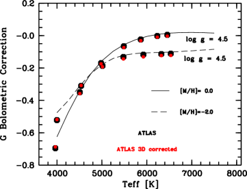
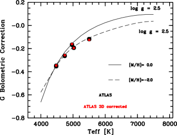
Figure 9: Bolometric corrections in the Gaia G band for four sets of models: log g = 2.5 (right panel) and log = 4.5 (left panel) at [M/H]=0.0 and [M/H]=–2.0. Black symbols are computed from our ATLAS models, the lines are the bolometric corrections computed from the Castelli & Kurucz (2003) grid. The solid line refers to models of solar metallicity, the dashed line to models with metallicity –2.0. The red symbols are the values to which we added the 3D correction.