First study of reionization in the Planck 2015 normalized closed $\Lambda$CDM inflation model

Abstract

We study reionization in two non-flat $\Lambda$CDM inflation models that best fit the Planck 2015 cosmic microwave background anisotropy observations, ignoring or in conjunction with baryon acoustic oscillation distance measurements. We implement a principal component analysis (PCA) to estimate the uncertainties in the reionization history from a joint quasar-CMB dataset. A thorough Markov Chain Monte Carlo analysis is done over the parameter space of PCA modes for both non-flat $\Lambda$CDM inflation models as well as the original Planck 2016 tilted, spatially-flat $\Lambda$CDM inflation model. Although both flat and non-flat models can closely match the low-redshift ($z\lesssim 6$) observations, we notice a possible tension between high-redshift ($z\sim 8$) Lyman-$\alpha$ emitter data and the non-flat models. This is solely due to the fact that the closed models have a relatively higher reionization optical depth compared to the flat one, which in turn demands more high-redshift ionizing sources and favors an extended reionization starting as early as $z\approx 14$. We conclude that as opposed to flat-cosmology, for the non-flat cosmology models (i) the escape fraction needs steep redshift evolution and even unrealistically high values at some redshifts and (ii) most of the physical parameters require to have non-monotonic redshift evolution, especially apparent when Lyman-$\alpha$ emitter data is included in the analysis.

1 Introduction

Measurements of the cosmic microwave background (CMB) anisotropy by the Planck satellite tightly constrain cosmological parameters (Planck Collaboration, 2016a). Their results are consistent with the standard spatially-flat $\Lambda$CDM inflation model (Peebles, 1984) whose leading current-epoch constituents are dark energy ($\sim 69\%$) in the form of a cosmological constant ($\Lambda$) and non-baryonic cold dark matter (CDM) ($\sim 26\%$). Six parameters are needed to describe this standard model, namely the physical baryonic density parameter ($\Omega_{\rm b}h^{2}$, where $h$ is the Hubble constant $H_{0}$ in units of 100 km/s/Mpc), the physical CDM density parameter ($\Omega_{\rm c}h^{2}$), the angular size of the sound horizon at recombination ($\theta$), the reionization electron scattering optical depth ($\tau_{\rm el}$), and the slope ($n_{s}$) and amplitude ($A_{s}$) of the (assumed) power-law primordial scalar energy density inhomogeneity power spectrum. Although the simple six-parameter tilted, spatially-flat $\Lambda$CDM model has proven to be successful on most observational fronts (Planck Collaboration, 2016a), some challenging issues still remain unsettled. For example, the uncertainty in the nature of dark energy persists till date (Peebles & Ratra, 1988; Ratra & Peebles, 1988; Sahni & Starobinsky, 2000; Padmanabhan, 2003; Sahni, 2004; Shafieloo, 2007; Ratra & Vogeley, 2008). Another issue is that local measurements of the expansion rate result in a higher $H_{0}$ (e.g., Riess et al., 2016) than many other techniques (Chen & Ratra, 2011; Calabrese et al., 2012; Sievers et al., 2013; Aubourg et al., 2015; Planck Collaboration, 2016a; L’Huillier & Shafieloo, 2017; Chen et al., 2017; Luković et al., 2016; Wang et al., 2017; Lin & Ishak, 2017; DES Collaboration, 2017; Yu et al., 2018).

Recently, it has been argued that a closed $\Lambda$CDM (or XCDM or $\phi$CDM) inflation model could partially alleviate two possible drawbacks of the tilted spatially-flat $\Lambda$CDM model (Ooba et al., 2017a, b, c). In the closed $\Lambda$CDM inflation model that best fits the Planck 2015 CMB anisotropy data, the predicted CMB temperature anisotropy angular power spectrum, $C_{\ell}$, where $\ell$ is multipole number, has less power at low $\ell$, in better agreement with the observations. Also, the resulting fractional energy density inhomogeneity averaged over 8$h^{-1}$ Mpc radius spheres, $\sigma_{8}$, is in better accord with lower estimates from weak lensing measurements. Both of these results are the consequence of the suppression of large-scale energy density inhomogeneity power in the best-fit closed inflation cases relative to the best-fit flat inflation model (Ooba et al., 2017a, b). However, the large $\ell$ $C_{\ell}$’s in the flat model provide a somewhat better fit to the observations than do those in the non-flat cases.

Nonzero spatial curvature provides an additional cosmological length scale so it is physically inconsistent to use a power-law energy density inhomogeneity power spectrum in a non-flat model. In a non-flat cosmological model inflation provides the only known way to compute the power spectrum. When the open inflation (Gott, 1982; Ratra & Peebles, 1994, 1995) and closed inflation (Hawking, 1984; Ratra, 1985, 2017) model energy density inhomogeneity power spectra are used to analyze the Planck CMB anisotropy data (Planck Collaboration, 2016a), they favor a closed Universe with current spatial curvature density parameter of magnitude of a percent or two (Ooba et al., 2017a, b, c).

More precisely, Ooba et al. (2017a) have analysed a six-parameter non-flat $\Lambda$CDM inflation model, parameterized by $\Omega_{\rm b}h^{2},\Omega_{\rm c}h^{2},\theta,\tau_{\rm el},\Omega_{\rm k}$ and $A_{s}$ (with previously considered free parameter $n_{s}$ now replaced by the current value of the spatial curvature density parameter $\Omega_{\rm k}$) by exploiting Planck 2015 CMB anisotropy (Planck Collaboration, 2016a) and baryon acoustic oscillation (BAO) distance measurements (Beutler et al., 2011; Anderson et al., 2014; Ross et al., 2015). They found that the existing data favour a slightly closed non-flat model with $\Omega_{\rm k}=-0.018\pm 0.008$ (1-$\sigma$ confidence limits; C.L.) when constrained against Planck CMB TT + lowP + lensing data alone, and with $\Omega_{\rm k}=-0.008\pm 0.002$ when the BAO data are included along with the Planck CMB measurements. In both cases, the resulting present day Hubble parameter $H_{0}$ and matter density parameter $\Omega_{\rm m}$ are compatible with most other data on these parameters. It might be significant that many analyses based on a variety of different non-CMB data (including BAO, Type Ia supernovae apparent magnitude, Hubble parameter, growth factor, and gravitational lensing data, as well as various combinations thereof) also do not rule out the non-flat models (Farooq et al., 2015; Sapone et al., 2014; Li et al., 2014; Cai et al., 2016; Chen et al., 2016; Yu & Wang, 2016; L’Huillier & Shafieloo, 2017; Farooq et al., 2017; Li et al., 2016; Wei & Wu, 2017; Rana et al., 2017; Yu et al., 2018).

However, Ooba et al. (2017a, b, c) find an interesting deviation from the original Planck results in another important aspect of observational cosmology, the value of the reionization optical depth $\tau_{\rm el}$, which has a direct influence on the epoch of reionization (EoR), because the transition from a neutral intergalactic medium (IGM) to an ionized one drastically increases the free electron contents that can Thomson scatter the CMB photons. For the tilted spatially-flat $\Lambda$CDM inflation model, Planck estimates $\tau_{\rm el}$ to be $0.066\pm 0.012$ from Planck 2015 (Planck Collaboration, 2016a) or $0.055\pm 0.009$ from Planck 2016 (Planck Collaboration, 2016b). The Planck flat-$\Lambda$CDM constraint points to an instantaneous reionization occurring at mean redshift $z_{\rm reion}\approx 8-9$ (Planck Collaboration, 2016c), which is compatible with reionization by the observed population of galaxies, namely PopII stars (Robertson et al., 2015; Mitra et al., 2015). A lower optical depth might also explain the rapid decrease in the number density of Ly$\alpha$ emitters (LAEs) detected at $z\sim 7$ which would have been in marginal tension with models having a relatively higher $\tau_{\rm el}$ (Mesinger et al., 2015; Choudhury et al., 2015). On the other hand, in the closed $\Lambda$CDM model Ooba et al. (2017a) reckon $\tau_{\rm el}$ to be quite high, which could have a severe impact on reionization at higher redshifts. Thus an in-depth investigation is needed on this aspect in order to address the significant differences between the higher-$z$ predictions for reionization in Planck 2016 normalized tilted flat-$\Lambda$CDM and Planck 2015 normalized closed-$\Lambda$CDM models.

This paper presents a first study of reionization in the non-flat $\Lambda$CDM inflation scenario. We put our emphasis on a detailed comparison between the flat and non-flat cosmological models. In the next section we briefly discuss the main features of our semi-analytical reionization model and the datasets used here to constrain it. We present our findings in Section 3, and finally conclude in Section 4.

2 Reionization model and datasets

The reionization model used here is based on the semi-analytical approach of Choudhury & Ferrara (2005) and Choudhury & Ferrara (2006b).

In this model, the ionization state of the IGM is well-described by a multi-phase medium, a mixture of both ionized and neutral regions. The density distribution of the IGM is assumed to have a lognormal form at low densities, changing to a power law at high densities (Choudhury & Ferrara, 2005). The model accounts for the inhomogeneities in the IGM using a description similar to that of Miralda-Escudé et al. (2000) in which reionization ends once all the low-density regions are ionized (Choudhury, 2009). For simplicity we assume that all photons are absorbed shortly after being emitted (this is commonly known as the “local source” approximation), which is a reasonable approximation for $z\gtrsim 3$ when the mean free path of photons is much smaller than the Hubble radius (Madau et al., 1999; Choudhury, 2009; Schirber & Bullock, 2003).

The ionizing ultra-violet (UV) photon budget is assumed to be produced by normal PopII stars and quasars. Many lines of evidence suggest that star-forming galaxies dominate the UV radiation background at earlier epochs, while quasars dominate only at later times due to the rapid decline in their abundances beyond $z\simeq 6$ (Hopkins et al. 2007; Kim et al. 2015; Mitra et al. 2018; D’Aloisio et al. 2017; Hassan et al. 2018; but also see Madau & Haardt 2015; Khaire et al. 2016 for quasar-only reionization models). The model also incorporates the impact of radiative feedback (which increases the minimum star-forming halo mass in the ionized regions) on reionization by altering the minimum circular velocity of halos that are able to cool. The production rate of ionizing photons is computed from

$$\dot{n}_{\gamma}=N_{\rm ion}n_{b}\frac{{\rm d}f_{\rm coll}}{{\rm d}t},$$ (1)

where $f_{\rm coll}$ is the fraction of matter that has collapsed into halos, obtained by using an appropriate halo mass function, $n_{b}$ is the total baryonic number density and $N_{\rm ion}$ is the number of ionizing photons in the IGM per baryon in stars, which can be written as a product of the star formation efficiency $\epsilon_{*}$, escape fraction $f_{\rm esc}$ of the ionizing photons escaping into the IGM and the specific number of photons emitted per baryon in stars, $N_{\rm ion}=\epsilon_{*}f_{\rm esc}N_{\gamma}$ (Mitra et al., 2013, 2015). In reality, this parameter depends on halo mass and redshift. Unfortunately, we do not have a physically motivated model for this, due to our limited understanding of complex star formation processes.

Here we ignore any explicit dependence of $N_{\rm ion}$ on halo mass. However, with the help of a principal component analysis (PCA), it is possible to include a redshift dependence (Mitra et al., 2011, 2012, 2015). The PCA technique has proven to be very useful in re-expressing a large number of (possibly) correlated variables in a new basis of a smaller number of uncorrelated variables without significant loss of information.

We start by assuming that $N_{\rm ion}(z)$ is an arbitrary function of $z$ and design the Fisher information matrix with help of a suitable fiducial model using the observed datasets of (i) the hydrogen photoionization rates $\Gamma_{\rm PI}$ in the range $2.4\leqslant z\leqslant 6$ from Wyithe & Bolton (2011) and Becker & Bolton (2013); (ii) redshift evolution of Lyman limit systems (LLS), ${\rm d}N_{\rm LL}/{\rm d}z$ over a wide redshift range ($0.36<z<6$) from the combined data points of Songaila & Cowie (2010) and Prochaska et al. (2010); and (iii) reionization optical depth $\tau_{\rm el}$ using three different constraints - a) recent Planck 2016 data ($0.055\pm 0.009$; flat $\Lambda$CDM model) from Planck Collaboration (2016b), b) non-flat $\Lambda$CDM with Planck 2015 CMB (TT + lowP + lensing) data ($0.101\pm 0.021$) and c) non-flat $\Lambda$CDM with Planck 2015 CMB + BAO data ($0.120\pm 0.012$) from Ooba et al. (2017a). The Fisher matrix thus contains information regarding the sensitivity of all the individual datasets on $N_{\rm ion}(z)$. The fiducial model $N_{\rm ion}^{\rm fid}(z)$ should be chosen in such a way that it can match all the observables at $z<6$ and also produce a $\tau_{\rm el}$ in the acceptable range. For the flat model we have taken a constant $N_{\rm ion}^{\rm fid}=10$ which is suited to match the Planck data as seen in Mitra et al. (2015). Unfortunately, this simplest constant model does not work for the non-flat cases, since we require larger contribution from early epoch sources in order to achieve higher $\tau_{\rm el}$ (also seen in Mitra et al. 2011, 2012). $N_{\rm ion}^{\rm fid}$ should be higher at early epochs where PopIII stars are likely to dominate and should smoothly transit to a lower value ($N_{\rm ion}^{\rm fid}=10$) at $z\lesssim 6$ determined by the usual PopII stars to produce a good match with all the observations considered in this work. Although the derived parameters somewhat depend on the fiducial model chosen, and the actual form of underlying true $N_{\rm ion}$ might be slightly different from it, the final conclusions of this paper (presented later) would hold for any $N_{\rm ion}^{\rm fid}$ which can produce at least a reasonable match with the observables mentioned above. We further set a prior on the neutral hydrogen fraction using robust constraints obtained from the Ly$\alpha$ forest observations of distant quasars by McGreer et al. (2015) at $z\sim 5-6$; $x_{\rm HI}<0.11$ at $z=5.9$ and $x_{\rm HI}<0.09$ at $z=5.6$. We kept all other cosmological parameters, corresponding to the different models, at their best-fit values as obtained by Planck Collaboration (2016a) for the flat model and by Ooba et al. (2017a) for the non-flat cases. For clarity, we quote those in Table 1. This means that the uncertainties on our reionization predictions here are tighter than they really should be; to account for the uncertainties on the other five cosmological parameters will require a more involved analysis.

Parameter	Flat model	Non-flat models
		TT+lowP+lensing	TT+lowP+lensing+BAO
$\Omega_{\rm m}$	$0.3089$	$0.32$	$0.28$
$\Omega_{\rm b}h^{2}$	$0.0223$	$0.02304$	$0.02302$
$\Omega_{\rm k}$	—	$-0.018$	$-0.008$
$h$	$0.6774$	$0.6433$	$0.6823$
$\sigma_{8}$	$0.8159$	$0.797$	$0.819$
$n_{s}$	$0.9667$	—	—

Table 1: List of the best-fit cosmological parameters for flat (from Planck Collaboration 2016a) and non-flat $\Lambda$CDM models (from Ooba et al. 2017a). We ignore uncertainties in these parameters in our analyses here.

Once we have the Fisher matrix, we can deconstruct it into pairs of eigenvalues and eigenvectors (also known as principal components, PCs). The primary objective of PCA is the dimensionality reduction of our fiducial parameter space. This can be done by identifying the more accurately determined modes with smaller uncertainties, which in turn correspond to the eigenmodes associated with larger eigenvalues. This results in a relatively fewer number of PCs needed for the reconstruction of the true $N_{\rm ion}(z)$. The other modes with larger uncertainties (or equivalently smaller eigenvalues) can be discarded at this stage without significant loss of information. We assume that PopII stars are the sole contributor of $N_{\rm ion}$; another stellar population, such as PopIII stars, might be expected to manifest itself as evolution of $N_{\rm ion}(z)$ with redshift (Mitra et al., 2011, 2012).

3 Results: MCMC-PCA constraints

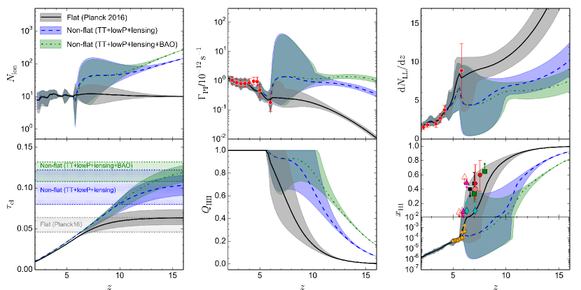
Figure 1: MCMC constraints on various quantities related to reionization history obtained from the PCA for three different cases: flat $\Lambda$CDM model with Planck 2016 data; non-flat $\Lambda$CDM with Planck 2015 CMB (TT + lowP + lensing) data and non-flat $\Lambda$CDM with TT + lowP + lensing + BAO data. The lines correspond to the best-fit models while the shaded regions correspond to their 2-$\sigma$ uncertainty ranges. The red points with error bars denote the corresponding observational data points. Top-left: the evolution of the effective $N_{\rm ion}(z)$; Top-middle: the hydrogen photoionization rate $\Gamma_{\rm PI}(z)$ along with observed data from Wyithe & Bolton (2011) and Becker & Bolton (2013); Top-right: the LLS distribution ${\rm d}N_{\rm LL}/{\rm d}z$ with combined data points from Songaila & Cowie (2010) and Prochaska et al. (2010); Bottom-left: electron scattering optical depth $\tau_{\rm el}$ and constraints from Planck Collaboration (2016b) and Ooba et al. (2017a) (indicated by differently shaded regions for the three different cases); Bottom-middle: the volume filling factor of HII regions $Q_{\rm HII}(z)$; Bottom-right: the global neutral hydrogen fraction $x_{\rm HI}(z)$ with various current observational limits. We direct the reader to Figure 6 for their references.

Constraints on $N_{\rm ion}(z)$ and other quantities are obtained from Markov Chain Monte Carlo (MCMC) analyses over the relevant principal modes using the datasets mentioned above. We find that the first $2-7$ eigenmodes with largest eigenvalues suffice for this purpose. The uncertainties derived from each mode are combined to determine the total uncertainty in the final stage of reconstruction by using a model-independent Akaike information criterion (Liddle, 2007). For details see Mitra et al. (2011, 2012, 2015). We repeat the whole analysis for all three cases considered here: flat $\Lambda$CDM and the two non-flat models with and without the BAO constraints.

The MCMC results are shown in Figure 1. The colored shaded regions and the lines, with different styles for different cases, correspond to the 2-$\sigma$ (95% C.L.) uncertainty ranges and mean values of those parameters, respectively, obtained from MCMC statistics. All quantities are tightly constrained at $z\lesssim 6$ as expected, due to the fact that most of the observed data related to reionization exist only at these redshifts. A wide range of histories at $z>6$ is still allowed by the data. The evolution at $z>6$ is essentially governed by the optical depth data alone, that’s why a relatively weaker constraint is apparent in this regime. The 2-$\sigma$ C.L. also shows a decreasing trend at high redshifts since the components of the Fisher matrix are zero as there exist no free electrons to contribute to $\tau_{\rm el}$, providing no significant information from the PCs beyond this point. The mean evolution of all the quantities for non-flat models is almost identical to the flat one at $z\lesssim 6$; at earlier epochs they differ significantly, as expected from the different electron scattering optical depths. The overall 2-$\sigma$ errors at $z>6$ on all quantities for non-flat models are slightly higher than those for the flat Planck 2016 model, as the observational uncertainty on the Planck 2016 $\tau_{\rm el}$ data is the lowest among the three models.

We find that, contrary to the flat Planck 2016 case, an evolving $N_{\rm ion}$ with redshift (top-left panel) is required for the non-flat Planck 2015 models due to higher values of $\tau_{\rm el}$. It is not possible to match this $\tau_{\rm el}$ data with a constant $N_{\rm ion}$, i.e. $N_{\rm ion}$ must increase at $z>6$ for these models. This is a clear signature of either a changing initial mass function (IMF) induced by chemical feedback from PopIII stars and/or evolution in the star-forming efficiency and/or evolution in the photon escape fraction of galaxies. These non-flat models show a relatively higher value of $\Gamma_{\rm PI}$ (top-middle panel) at early epochs than the flat model, as the former ones allow the contribution of ionizing photons from high-redshift PopIII stars. In fact, the PopIII photon contribution seem to be highest for the non-flat CMB + BAO case, as $\tau_{\rm el}$ for this model is the largest of all. A similar trend is also found in the evolution of LLSs (top-right panel). In both panels we indicate the corresponding current observational constraints (red points with error bars) at $z\lesssim 6$ which we have included in this MCMC analysis. All three models match these quite accurately. Another key quantity of interest is the volume filling factor $Q_{\rm HII}(z)$ for ionized hydrogen (HII) regions which is basically the fraction of the IGM volume that is occupied by ionized regions. From its evolution (bottom-middle panel), one can see that reionization is almost completed ($Q_{\rm HII}\sim 1$) around $5.8\lesssim z\lesssim 7.5$ (2-$\sigma$ limits) for the flat Planck 2016 model. The mean ionized fraction evolves quite rapidly, whereas the mean non-flat models favor a relatively gradual or extended reionization starting as early as $z\approx 14$. Higher the $\tau_{\rm el}$, the more extended is the reionization process. This is also reflected in the evolution of the neutral hydrogen fraction $x_{\rm HI}(z)$ (bottom-right panel). Here we also show various observational limits on $x_{\rm HI}(z)$ (points with different colors) based on the measurements of quasar absorption lines, Ly$\alpha$ emitters, gamma-ray bursts (GRBs) etc. (see Section 3.3 for details). We did not include these datasets, except the most robust limits (open triangles) at $z\sim 5-6$ from McGreer et al. (2015), as constraints in our analyses.

We note that the TT + lowP + lensing + BAO analyses of the non-flat XCDM inflation model (Ooba et al., 2017b) and of the non-flat $\Lambda$CDM inflation model (Ooba et al., 2017a) result in almost identical constraints on cosmological parameter central values, with the central value of the XCDM equation of state parameter being $w_{0}=-1$, This means that for this CMB and BAO dataset our non-flat $\Lambda$CDM reionization results also apply to the non-flat XCDM model.

3.1 UV luminosity function

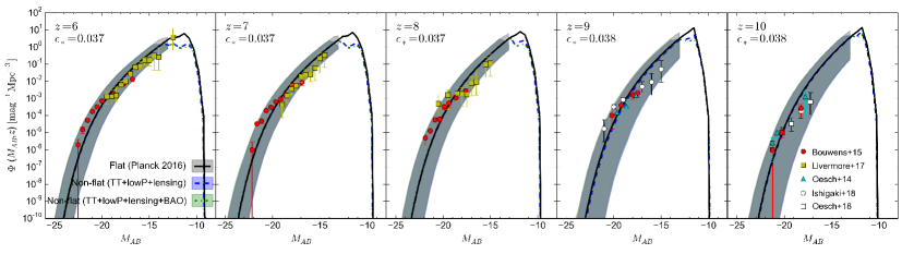
Figure 2: Evolution of high redshift ($z=6-10$) galaxy luminosity function for different models (flat $\Lambda$CDM and two non-flat models with and without the BAO constraints) with best-fit $\epsilon_{*}$ and the 2-$\sigma$ limits (shaded regions). The data points with errorbars correspond to currently available observational constraints, see the text for their references.

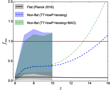
Figure 3: Redshift evolution of the escape fraction along with its 2-$\sigma$ errors for different models considered in this work. The red solid line indicates an escape fraction of unity. For $z>10$, where no observations on galaxy luminosity function exist, only the best-fit models are shown.

Redshift	best-fit $f_{\rm esc}$ [2-$\sigma$ C.L.]
	Flat	Non-flat (TT+lowP+lensing)	Non-flat (TT+lowP+lensing+BAO)
$z=6$	$0.0927$ $[0.0255,0.1702]$	$0.0853$ $[0.0213,0.1437]$	$0.0851$ $[0.0212,0.1434]$
$z=7$	$0.0998$ $[0.0393,0.2093]$	$0.3125$ $[0.1713,1.1628]$	$0.2984$ $[0.1620,1.0052]$
$z=8$	$0.0998$ $[0.0403,0.2139]$	$0.3731$ $[0.1904,1.3059]$	$0.3561$ $[0.1886,1.1759]$
$z=9$	$0.0979$ $[0.0324,0.2203]$	$0.3686$ $[0.1499,1.2198]$	$0.3669$ $[0.1500,1.1329]$
$z=10$	$0.0976$ $[0.0272,0.2359]$	$0.3817$ $[0.1233,1.2165]$	$0.4163$ $[0.1268,1.1986]$

Table 2: The derived best-fit values and 2-$\sigma$ C.L. of the escape fraction for different reionization models at redshifts $z=6-10$.

Given the very high $N_{\rm ion}$ values and their strong evolution with redshift needed for non-flat models, one should check whether the escape fraction needed for PopII stars becomes unrealistically high at some redshifts. $f_{\rm esc}$ can be obtained by combining the reionization histories and the evolution of the galaxy UV Luminosity Function (LF). This has already been studied in many of the earlier works, see e.g., Samui et al. (2007, 2009); Kulkarni & Choudhury (2011); Mitra et al. (2013, 2015). We refer the reader to these references for the methodology. The basic idea is to calculate the LF ($\Phi(M_{AB},z)$; $M_{AB}$ being the absolute AB magnitude) at redshift $z$ from the luminosity at $1500$ $\mathring{\rm A}$ of a galaxy which depends on the star-forming efficiency of PopII stars $\epsilon_{*}$. We then vary $\epsilon_{*}$ as a free parameter and match the observed LFs at redshifts $z=6-10$.

In Fig. 2, we present our results of the best-fit $\epsilon_{*}$ with $95\%$ C.L. for all three different reionization models (indicated by the same color code as in Figure 1) considered in this work. The observational datasets used here are from Bouwens et al. (2015a) for redshifts $z=6$ to $10$ (red filled circles); Livermore et al. (2017) for galaxies at $z=6-8$ (yellow filled squares); Oesch et al. (2014) and Oesch et al. (2018) for redshift $9-10$ galaxy candidates (filled cyan triangles and open squares respectively); and Ishigaki et al. (2018) for $z=9$ (open circles). Although the match between data and model predictions is quite satisfactory for all redshifts considered here, a better match can be achieved by considering a mass-dependent $\epsilon_{*}$ and/or correction due to dust or halo mass quenching (Peng et al., 2010) in the analysis which is beyond the ambit of this paper. We find that the best-fit $\epsilon_{*}$ remains roughly constant ($\sim 4\%$) throughout the redshift range for all the models.

Once $\epsilon_{*}$ is known for different redshifts, we can obtain limits for $f_{\rm esc}$ using the MCMC constraints on the evolution of $N_{\rm ion}(z)$. Remember that, $N_{\rm ion}=\epsilon_{*}f_{\rm esc}N_{\gamma}$ where $N_{\gamma}\approx 3200$ for the PopII Salpeter IMF assumed here. The resulting $f_{\rm esc}$ values for different models are shown in Table 2 and Figure 3. The 2-$\sigma$ uncertainties in $f_{\rm esc}$ have been calculated using the quadrature method (Mitra et al., 2013). As the star-formation efficiency is almost the same from $z=6$ to $10$, we can assume that it will remain constant at $4\%$ even at $z>10$ and estimate the best-fit $f_{\rm esc}$ at those redshifts. This is a reasonable assumption in the absence of galaxy luminosity function observations beyond redshift $10$. Note that, in this figure we have shown the 2-$\sigma$ limits on $f_{\rm esc}$ only at $z=6-10$ where the corresponding LF observables are available, whereas at $z>10$ we just extend its best-fit values using an $\epsilon_{*}\approx 0.04$ and best-fit $N_{\rm ion}(z)$ from the MCMC. We find that the best-fit escape fraction remains constant at $\sim 10\%$ for the whole redshift range in the flat $\Lambda$CDM case, whereas a strong redshift evolution of this quantity is required for the two non-flat models – it increases by a factor of $\sim 5$ from $z=6$ to $10$ and approaches values as high as $\sim 100\%$ at $z\approx 15$ for model without the BAO constraints (or $200\%$ in case of with-BAO model). This also explains why the Universe is significantly ionized ($10-20\%$) even at $z\sim 15$ in these non-flat models (see the plot for $x_{\rm HI}$). Interestingly, if we look at the 2-$\sigma$ ranges, these two non-flat models can lead to this impractically high $f_{\rm esc}$ ($\gtrsim 1$) even at redshifts $z\approx 7$. This is solely due to the fact that $N_{\rm ion}$ for non-flat models can become as high as $\sim 150$ at $z=7$, considering its 2-$\sigma$ limits (see the top-left panel of Figure 1), in order to produce such high reionization optical depths. However, it is not possible to rule out these models based on these considerations alone as a wide range of reionization history is still allowed at $z=7-10$ for these models due to lack of good quality data at $z\gtrsim 7$. This is also reflected in the plot of $x_{\rm HI}$ in Figure 1. In the following section, we shall see how this situation can be improved by adding constraints from LAEs in our analysis.

A similar strong $f_{\rm esc}(z)$ evolution for higher reionization optical depths and this striking one-to-one correspondence between them have been reported earlier. For example, Haardt & Madau (2012) found that $f_{\rm esc}$ increases towards higher redshifts and it becomes unity by $z\approx 12$ for their minimal reionization model. They also argued that if a maximum $f_{\rm esc}$ of $50\%$ was assumed, the same model can yield a much lower $\tau_{\rm el}=0.06$. Kuhlen & Faucher-Giguère (2012) claimed that a strong increase of $f_{\rm esc}$ from $\sim 4\%$ at $z=4$ to $1$ at earlier times is needed for their reionization model to match WMAP7 $\tau_{\rm el}$ of $0.088$ (also see their Figure 5 for a direct correlation between optical depth and a constant $f_{\rm esc}$; higher value of $f_{\rm esc}$ can result in a larger $\tau_{\rm el}$). In our earlier work (Mitra et al., 2013) we also found an increasing escape fraction towards higher redshifts in order to produce the desired WMAP7 $\tau_{\rm el}$ value. However, we noted that for our model it is possible to satisfy WMAP7 and LF data simultaneously without requiring an escape fraction of order of unity at earlier epochs, the upper limits of $f_{\rm esc}$ need be at most $50\%$ at $z=8$.

3.2 Inclusion of neutral fraction measurements from Ly$\alpha$ transmission at $z\sim 7$

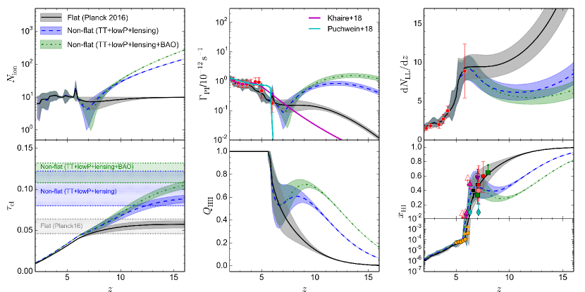
Figure 4: Same as Figure 1, but now including $x_{\rm HI}$ constraint at $z\sim 7$ from Mason et al. (2018) indicated by filled purple pentagon in the bottom-right panel. See Figure 6 for the complete references of $x_{\rm HI}$ constraints.

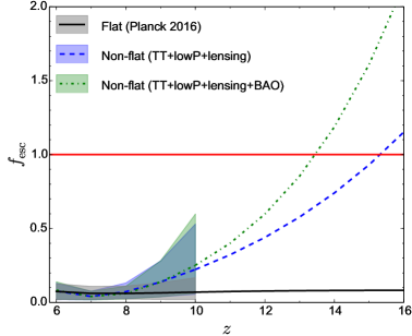
Figure 5: Same as Figure 3, but now including $x_{\rm HI}$ constraint at $z\sim 7$ from Mason et al. (2018).

Redshift	best-fit $f_{\rm esc}$ [2-$\sigma$ C.L.]
	Flat	Non-flat (TT+lowP+lensing)	Non-flat (TT+lowP+lensing+BAO)
$z=6$	$0.0741$ $[0.0190,0.1260]$	$0.0771$ $[0.0193,0.1300]$	$0.0826$ $[0.0206,0.1392]$
$z=7$	$0.0610$ $[0.0216,0.1081]$	$0.0403$ $[0.0170,0.0762]$	$0.0402$ $[0.0166,0.0756]$
$z=8$	$0.0610$ $[0.0225,0.1108]$	$0.0724$ $[0.0261,0.1317]$	$0.0595$ $[0.0223,0.1099]$
$z=9$	$0.0645$ $[0.0109,0.1333]$	$0.1383$ $[0.0375,0.2809]$	$0.1387$ $[0.0375,0.2816]$
$z=10$	$0.0696$ $[0.0184,0.1672]$	$0.2225$ $[0.0545,0.5299]$	$0.2510$ $[0.0613,0.5975]$

Table 3: Same as Table 2, but now including $x_{\rm HI}$ constraint at $z\sim 7$ from Mason et al. (2018).

So far the reionization histories at $z>6$ depend only on the value of $\tau_{\rm el}$ coming from CMB observations, and thus the constraints remain relatively weaker at those redshifts. One can, in principle, include other high-redshift non-CMB datasets in order to further strengthen the model constraints. We have indicated some of those possibilities in the plot for $x_{\rm HI}$ (or see Section 3.3 for details). Although these data are highly model-dependent and might get modified in the future, it would be interesting to check if the constraints improve significantly by including such measurements available at $z>6$. To this end, here we have included one more observable, the constraint on the global neutral fraction at $z\sim 7$ of $x_{\rm HI}=0.59^{+0.11}_{-0.15}$ from Mason et al. (2018), in addition to the earlier datasets mentioned in Section 2. This data is inferred from a sample of observed Lyman Break galaxies (LBGs) presented in Pentericci et al. (2014) using a Bayesian inference framework and sophisticated IGM simulations.

The resulting reionization constraints are shown in Figure 4. The first thing to note is that the 2-$\sigma$ limits are considerably reduced for all the models considered here since we now force the model to match the $x_{\rm HI}$ constraint. Such high value of $x_{\rm HI}$ at $z=7$ essentially disfavours a large set of models which were otherwise allowed in our earlier analysis. Although we still require a similar strong redshift evolution of $N_{\rm ion}$ for the non-flat cases, the rise is rather late, starting at $z>8$ and then rapidly increasing towards higher redshifts. This indicates that the PopII stars dominate the reionization over a longer period of time up to $z\approx 8$ and after that a sharp increase in photon escape fraction and/or the PopIII stars take over, so that enough contribution to $\tau_{\rm el}$ is acquired to match its corresponding value. However, all these models produce somewhat lower $\tau_{\rm el}$ than what we got earlier, reflecting a possible tension between high-$z$ LAE data and a very large optical depth value ($\gtrsim 0.11$). In fact, we find that the best-fit $\chi^{2}$-values increase by $\sim 2.5$ for the non-flat models when the additional LAE constraint is included in the analysis (the corresponding rise in the best-fit $\chi^{2}$ is only $0.7$ for the flat model). This indicates that the non-flat models tend to perform worse in presence of the LAE constraint, however, they cannot still be conclusively ruled out because of the large error-bars in the data.

The constraints on $Q_{\rm HII}$ and $x_{\rm HI}$ change significantly in this case, in particular they become very constricted near the end-stage of reionization. Reionization is almost completed ($Q_{\rm HII}\sim 1$) at $5.8\lesssim z\lesssim 6.0$ (2-$\sigma$ limits) irrespective of the model we choose. Hence, if we include the $x_{\rm HI}$ measurements at $z\gtrsim 7$ in the analysis, completion of reionization cannot occur earlier than $z\approx 6$, essentially ruling out most of the models of early reionization which were allowed previously. The growth of $Q_{\rm HII}$ is gradual for the flat model. On the other hand, the non-flat models, which are characterized by a sharp rise in $N_{\rm ion}$ and $\Gamma_{\rm PI}$ at $z>8$ in order to produce high optical depths, indicate a much faster increase in $Q_{\rm HII}$ at initial stages, followed by a sharp fall around $z\approx 8$ (corresponding to a sharp decrease in $N_{\rm ion}$) to match the $x_{\rm HI}$ measurements (filled purple pentagon in the plot). Similar conclusions can be obtained from the plot of neutral fraction. For the non-flat models, it shows a gradual decrease up to $z\sim 8$ from its higher value at earlier redshifts, then a rapid increase up to $z\approx 7$ in order to obey the observed $x_{\rm HI}$ limit and finally it decreases again to smoothly match the Ly$\alpha$ forest data at $z\lesssim 6$.

Although the inclusion of LAE data reduces the tension between the predicted $x_{\rm HI}$ from non-flat models with the observed value at $z\sim 7$, it now introduces a clear non-monotonic redshift evolution of photoionization rates, LLSs and the neutral fraction. It will be very difficult for any physically motivated reionization model to justify such trends like the sudden decrease in LLSs at $z>6$ (corresponding to an abrupt increase in mean-free path of ionizing photons around this redshift) or the recombination of hydrogen again at $z\sim 6-9$. Also such rapid boost in the evolution of photoionization rates at $z>7$ lacks a meaningful explanation and cannot be naturally produced by any UV background model. For comparison we have plotted here the $\Gamma_{\rm PI}$ evolution predicted by two recent models from Khaire & Srianand (2018) (solid purple curve) and Puchwein et al. (2018) (cyan curve) which clearly shows the opposite trends. In fact, the monotonic evolution of $\Gamma_{\rm PI}$ from the flat CDM case is somewhat more agreeable with their results.

Next we try to fit the observed UV luminosity functions at $z=6-10$ following the same method described in Section 3.1, and the results are almost similar to those obtained from our previous analysis (Figure 2). The same non-evolving SF efficiency of $\epsilon_{*}\approx 4\%$ is required for all redshift ranges. However the constraints on $f_{\rm esc}$ at $z=6-10$ modify considerably (shown in Figure 5 and Table 3) due to the change in $N_{\rm ion}$. The escape fraction remains unchanged at $\approx 10\%$ for $z\lesssim 8$ in all the models reflecting the non-evolving nature of $N_{\rm ion}$ at those redshifts. Then it increases moderately towards redshift $z\approx 10$ for non-flat cases. In particular, for the model with highest $\tau_{\rm el}$ a maximum of $60\%$ (2-$\sigma$ C.L.) photon escape fraction is needed at redshift $10$. Unlike the previous case, now the non-flat models do not require unrealistically high value of $f_{\rm esc}$ at $z\lesssim 10$. This is because the inclusion of the $z\sim 7$ $x_{\rm HI}$ constraint forces these models to a relatively late reionization scenario reducing the need of significantly higher amount of early epoch ($6\lesssim z\lesssim 10$) sources or very large PopII escape fractions. But we still need the best-fit $f_{\rm esc}$ to be $\gtrsim 1$ at higher redshifts, as a very high $N_{\rm ion}$ ($>100$) at $z\gtrsim 13$ is required for these non-flat models to match the corresponding optical depth constraints.

Nonetheless, we should mention that the inferred $x_{\rm HI}$ measurements from high-$z$ LAEs can have model dependencies and large uncertainties, e.g., effects of dust extinction (Dayal et al., 2009), self-shielded absorbers (Bolton & Haehnelt, 2013; Choudhury et al., 2015; Kakiichi et al., 2016; Weinberger et al., 2018), or infall of circumgalactic medium (CGM) matter in the haloes (Sadoun et al., 2017; Weinberger et al., 2018). Thus any conclusions drawn by incorporating them in our analysis should be interpreted with caution.

3.3 Comparison of the results with other data

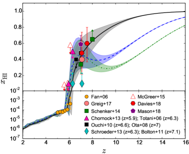
Figure 6: Bottom-right panel of Figure 4 – evolution of the neutral hydrogen fraction compared with various existing observations listed here and described further in the text.

Finally, we focus on the comparison of our model predictions for the neutral fraction ($x_{\rm HI}$) with other data. A separate plot for $x_{\rm HI}$ from the analysis presented in the last section is shown in Figure 6 (same as the bottom-right panel of Figure 4) for clarity. Although the majority of the data shown in this figure provide weak and model-dependent constraints on the EoR, it is instructive to compare our model predictions with these data.

• Quasars: The strongest evidence related to reionization perhaps comes from the Ly$\alpha$ forest data of high-redshift quasars from Fan et al. (2006b). However, estimating the volume-averaged neutral fraction from the original data involves adoption of a particular model of IGM density distribution and temperature evolution. From the evolution of $x_{\rm HI}(z)$, one can immediately see a striking match between all our models and these data, shown here by filled yellow circles, even though we did not use these data in our MCMC analyses. This is not unexpected for the following reason. Fan et al. (2006b) assume a simple parametric form for the density distribution function (Miralda-Escudé et al., 2000) which is qualitatively very similar to the lognormal distribution adopted here (Mitra et al., 2015). Also their IGM inhomogeneities are calculated from the evolution of the mean free path using the same Miralda-Escudé et al. (2000) prescription we use in our model. Other evidence comes from the observations of quasar near zones. Bright quasars at early epochs ($z\sim 6-7$) can create the largest ionized regions around them, known as near zones, and thus can have a prominent effect on the IGM at the tail-end of reionization (Bolton & Haehnelt, 2007b; Carilli et al., 2010; Padmanabhan et al., 2014). Recent measurements of these at $z\sim 6.3$ by Schroeder et al. (2013) and at $z\sim 7.1$ by Bolton et al. (2011) infer a corresponding lower limit on mean $x_{\rm HI}\gtrsim 0.1$ (filled cyan diamonds in the figure). More recently, Greig et al. (2017) and Davies et al. (2018) constrained the neutral fraction from the damping wing analysis of highest redshift ($z>7$) quasars known. The mean $x_{\rm HI}=0.40^{+0.21}_{-0.19}$ at $z=7.09$ from Greig et al. (2017) and $x_{\rm HI}=0.60^{+0.20}_{-0.23}(0.48^{+0.26}_{-0.26})$ at $z=7.54(7.09)$ from Davies et al. (2018) are shown here by filled salmon circle and red hexagons respectively. However, there could be several ambiguities in estimating these constraints due to our poor understanding of the intrinsic properties of observed quasars (Bolton & Haehnelt, 2007a; Maselli et al., 2007), and hence these have not been used here for constraining our model parameters. More useful constraints for us instead come from a model independent dark pixel analysis of high-$z$ quasar spectra by McGreer et al. (2015), especially the upper limits at $z\sim 5.6$ and $5.9$ (open red triangles). We ensure our models not defy these bounds by imposing a prior in the MCMC analysis, which guarantees that reionization is almost completed at least by redshift $\sim 5.8$.

• Gamma-ray bursts: The afterglow spectra of gamma-ray bursts (GRBs) is another potential probe of the EoR (Bromm & Loeb, 2006). We show the constraints from observed GRB host galaxies of $x_{\rm HI}\lesssim 0.5$ at $z\sim 6.3$ (Totani et al., 2006) and $x_{\rm HI}\lesssim 0.1$ at $z\sim 5.9$ (Chornock et al., 2013) by filled pink triangles. Although these data are relatively weak due to the intrinsic damped Ly$\alpha$ absorption, predictions from all our models, interestingly, quite reasonably obey these limits.

• Ly$\alpha$ emitters: As the number densities of observed quasars and GRBs decline at high redshifts, one must look at the next higher-redshift reliable probe of the EoR, the Ly$\alpha$ emitters (LAEs). Studies of Lyman$\alpha$ emitting galaxies near the end of the EoR have proven crucial for understanding reionization processes, because of the attenuation of Ly$\alpha$ emission lines by neutral contents left in the IGM at this epoch (Ouchi et al., 2009). Observations of LAEs at $z=6.6$ by Ouchi et al. (2010) and at $z=7$ by Ota et al. (2008) infer the values of $x_{\rm HI}$ to be $\lesssim 0.4$ and $0.32-0.64$ respectively (shown in the plot by filled black squares). More recently, Schenker et al. (2014) have presented the most promising measurements of Ly$\alpha$ emission at the highest redshift known and provide an estimate of neutral fraction to be $x_{\rm HI}=0.34^{+0.09}_{-0.12}$ at $z\sim 7$ and $x_{\rm HI}>0.65$ at $z\sim 8$ (filled green squares). The resulting 2-$\sigma$ MCMC limits on this quantity from our non-flat models seem to be significantly low at this redshift; it can take values at most $\sim 0.5$ at $z=8$. Choudhury et al. (2015), using simulations of the high-redshift IGM, showed that the evolution in the LAE number density at $z\gtrsim 6.6$ is in better agreement with reionization models having $\tau_{\rm el}\lesssim 0.066$. Even though there might exist several uncertainties in the estimation of $x_{\rm HI}$ and reionization history from LAE data, we can say that the most severe challenges for the non-flat models come from these datasets. On the other hand, the lower $\tau_{\rm el}$ data for flat model makes it possible to produce a moderate evolution of $x_{\rm HI}$ in agreement with the current observed limits for all redshifts.

The fact that a model with a higher reionization optical depth produces a considerably smaller neutral fraction at earlier times has been reported earlier (Robertson et al., 2013; Robertson et al., 2015; Bouwens et al., 2015b; Mitra et al., 2015). In particular, Robertson et al. (2015) demonstrated that it is possible to simultaneously match the lower $\tau_{\rm el}$ from Planck 2015 and most of the observed constraints on $x_{\rm HI}$ in the range $6\lesssim z\lesssim 8$ using the latest Hubble Space Telescope data on the star formation rate density $\rho_{\rm SFR}(z)$. However a model with a higher $\tau_{\rm el}$ (e.g. $0.088$ from nine years of Wilkinson Microwave Anisotropy Probe or WMAP9 observations) would require a dramatic increase of SFR at $z\gtrsim 7.5$ and hence lead to a notable inconsistency with several observations on the neutral fraction. In fact, a very similar trend can also be seen in their earlier work (Robertson et al., 2013) where they showed that a model that matches the observed $x_{\rm HI}$ quite well struggles to produce such a large WMAP9 $\tau_{\rm el}$ value.

4 Concluding remarks

We have presented a detailed statistical analysis of reionization in closed $\Lambda$CDM inflation models using joint datasets of CMB and quasars. In particular, we compare how reionization proceeded over cosmic time in the flat and non-flat models. In the non-flat models under consideration the cosmological parameters are constrained by the Planck 2015 CMB data (also in combination with the BAO measurements) using a consistent energy density inhomogeneity power spectrum (Ooba et al., 2017a). These data prefer mildly closed ($\Omega_{\rm k}<0$) models with the curvature density parameter contributing only $1\%-2\%$ of the total mass-energy budget of the Universe. Such models not only reasonably match many observations but might also improve the agreement with observed low-$\ell$ $C_{\ell}$’s and weak lensing determined $\sigma_{8}$’s, although they do somewhat worsen the high-$\ell$ $C_{\ell}$ fit. However, these models predict a relatively higher reionization optical depth than that found from Planck 2016 data with the spatially-flat tilted $\Lambda$CDM model. This could result in a completely different reionization history at earlier epochs ($z>6$) in the non-flat cases.

Our main results, in summary, are:

• We find all three models behave the same way in the lower redshift regime ($z\lesssim 6$), as expected, whereas their predictions at higher-$z$ depart from each other due to the differences in optical depth values.

• Unlike the flat case, the non-flat models need many more high redshift reionization sources. A changing IMF influenced by PopIII stars and a strong evolution in the photon escape fraction of galaxies are two possibilities.

• For the usual flat model from Planck 2016, the lower optical depth favors a relatively quicker evolution of reionization. On the other hand, a more gradual or extended reionization is found for the non-flat models. In fact, larger the optical depth, more gradual is the reionization process.

• The resulting neutral hydrogen fraction seems to be quite small at higher redshifts ($z>7$) for the non-flat models compared to the flat one. Such small values, e.g. $\lesssim 0.4$ at $z\sim 8$, are likely disfavored by current observational bounds from distant Ly$\alpha$ emitters.

• This also reflects in the evolution of escape fraction. $f_{\rm esc}$ must be higher at earlier epochs for the non-flat models. The best-fit $f_{\rm esc}$ increases from $\sim 10\%$ at $z=6$ to $\sim 40\%$ at $z=10$, and up to $>100\%$ at much higher redshifts, and considering its 2-$\sigma$ limits it can become unrealistically high ($>1$) even at $z\gtrsim 7$. On the other hand, a constant escape fraction of $\sim 10\%$ is sufficient for the flat $\Lambda$CDM model.

One can see that, apart from the constraint on $x_{\rm HI}$ at $z\sim 8$ (filled square lower limit point in bottom-right panel of Fig. 1), the non-flat models, considering their 2-$\sigma$ limits, are not yet in conflict with most of the measurements related to reionization. The $z\sim 8$ data comes from the recent estimates of evolving LAEs by Schenker et al. (2014). Those observational results are then converted to $x_{\rm HI}$ by adopting a suitable model appropriate for patchy reionization (McQuinn et al., 2007; Schenker et al., 2012). This conversion however involves modeling several uncertain key parameters, like the escape fraction of ionizing photons, the degree of self-shielding etc. and by necessity this will bring in model dependencies. In fact, most of the observed $x_{\rm HI}$ constraints at $z\gtrsim 7$ are somewhat model dependent, hence we did not include them in the main MCMC analysis. Nevertheless, in order to examine how the non-flat models perform if one uses such data to constrain the reionization history, we later included the observed $x_{\rm HI}$ at $z\sim 7$ from Mason et al. (2018) keeping in mind that the results might be significantly biased by uncertainties in interpreting the data. The resulting 2-$\sigma$ limits at $z>6$ now reduce considerably for all the models due to this additional high redshift data. For non-flat scenarios $N_{\rm ion}$ remains constant up to $z\approx 8$, then increases rapidly at higher redshifts. In fact it behaves somewhat similar to the lower bound of $N_{\rm ion}$ plotted in Figure 1, which signifies that the PopII stars remain dominating until $z\sim 8$ in order to match the $x_{\rm HI}$ constraint included here. As a result we get an almost constant $f_{\rm esc}$ of $\sim 10\%$ up to $z=8$ with moderately increasing (maximum of $60\%$ for 2-$\sigma$ limits) towards $z=10$, indicating that the non-flat models are still permitted by the LBG data at $z\sim 7$. However if we continue to higher redshifts, assuming the same constant $4\%$ SF efficiency, where no actual observations on galaxy LF exist, the best-fit $f_{\rm esc}$ can again become unrealistically high for these models. Also, the evolution of various reionization quantities (e.g. photoionization rate, LLSs, neutral fraction etc. from Figure 4) becomes significantly non-monotonic in nature, especially when we include the LAE data. It will not be straightforward for any physical model to account for such trends. Interestingly, we find that the non-flat models perform much worse in terms of the best-fit $\chi^{2}$ when the LAE constraints are included, however, the error-bars are not small enough to rule them out.

Although it is now well understood that the LAE data prefer a late reionization (Mesinger et al., 2015; Choudhury et al., 2015) and the non-flat models struggle to match this, we still probably have to rely on upcoming observations on high-redshift reionization sources to conclusively rule out the non-flat models. Finally, we end this paper by indicating some, likely to be decisive, future observational prospects in this regard.

In the next few years there will be excellent openings on various observational fronts for greatly improving our understanding of the end phases of the EoR. Future observations of more high-redshift quasars are expected to come from the Large Synoptic Survey Telescope (LSST), Euclid, the Wide-Field Infrared Survey Telescope (WFIRST), the Thirty Meter Telescope (TMT) and the Giant Magellan Telescope (GMT), which can significantly increase our knowledge on the timing and nature of reionization. Furthermore, the James Webb Space Telescope (JWST), the Atacama Large Millimeter Array (ALMA) and the Hyper Suprime-Cam (HSC) on the Subaru telescope seem to be most promising instruments to target high-redshift LAEs as a very powerful reionization probe. And finally, the detection of the redshifted 21-cm signal from the EoR by several radio telescopes like the Giant Metrewave Radio Telescope (GMRT), the Murchison Widefield Array (MWA), the Hydrogen Epoch of Reionization Array (HERA) and the Low-Frequency Aperture Array (LFAA) of the Square Kilometre Array (SKA) will provide direct probes of the ${\rm HI}$ distribution in the diffuse IGM, which should be able to adjudicate between the different reionization scenarios of the flat and non-flat models.

References

- Anderson et al. (2014) Anderson L., et al., 2014, MNRAS, 441, 24
- Aubourg et al. (2015) Aubourg É., et al., 2015, Phys. Rev. D, 92, 123516
- Barkana & Loeb (2001) Barkana R., Loeb A., 2001, Phys. Rep., 349, 125
- Becker & Bolton (2013) Becker G. D., Bolton J. S., 2013, MNRAS, 436, 1023
- Beutler et al. (2011) Beutler F., et al., 2011, MNRAS, 416, 3017
- Bolton & Haehnelt (2007a) Bolton J. S., Haehnelt M. G., 2007a, MNRAS, 374, 493
- Bolton & Haehnelt (2007b) Bolton J. S., Haehnelt M. G., 2007b, MNRAS, 381, L35
- Bolton & Haehnelt (2013) Bolton J. S., Haehnelt M. G., 2013, MNRAS, 429, 1695
- Bolton et al. (2011) Bolton J. S., et al., 2011, MNRAS, 416, L70
- Bouwens et al. (2015a) Bouwens R. J., et al., 2015a, ApJ, 803, 34
- Bouwens et al. (2015b) Bouwens R. J., Illingworth G. D., Oesch P. A., Caruana J., Holwerda B., Smit R., Wilkins S., 2015b, ApJ, 811, 140
- Bromm & Loeb (2006) Bromm V., Loeb A., 2006, ApJ, 642, 382
- Cai et al. (2016) Cai R.-G., Guo Z.-K., Yang T., 2016, Phys. Rev. D, 93, 043517
- Calabrese et al. (2012) Calabrese E., Archidiacono M., Melchiorri A., Ratra B., 2012, Phys. Rev. D, 86, 043520
- Carilli et al. (2010) Carilli C. L., et al., 2010, ApJ, 714, 834
- Chen & Ratra (2003) Chen G., Ratra B., 2003, Publ. Astr. Soc. Pac., 115, 1143
- Chen & Ratra (2011) Chen G., Ratra B., 2011, Publ. Astr. Soc. Pac., 123, 1127
- Chen et al. (2016) Chen Y., Ratra B., Biesiada M., Li S., Zhu Z.-H., 2016, ApJ, 829, 61
- Chen et al. (2017) Chen Y., Kumar S., Ratra B., 2017, ApJ, 835, 86
- Chornock et al. (2013) Chornock R., et al., 2013, ApJ, 774, 26
- Choudhury (2009) Choudhury T. R., 2009, Current Science, 97, 841
- Choudhury & Ferrara (2005) Choudhury T. R., Ferrara A., 2005, MNRAS, 361, 577
- Choudhury & Ferrara (2006a) Choudhury T. R., Ferrara A., 2006a, preprint, (arXiv:astro-ph/0603149)
- Choudhury & Ferrara (2006b) Choudhury T. R., Ferrara A., 2006b, MNRAS, 371, L55
- Choudhury et al. (2015) Choudhury T. R., Puchwein E., Haehnelt M. G., Bolton J. S., 2015, MNRAS, 452, 261
- Clarkson & Zunckel (2010) Clarkson C., Zunckel C., 2010, Physical Review Letters, 104, 211301
- D’Aloisio et al. (2017) D’Aloisio A., Upton Sanderbeck P. R., McQuinn M., Trac H., Shapiro P. R., 2017, MNRAS, 468, 4691
- DES Collaboration (2017) DES Collaboration 2017, preprint, (arXiv:1711.00403)
- Davies et al. (2018) Davies F. B., et al., 2018, preprint, (arXiv:1802.06066)
- Dayal et al. (2009) Dayal P., Ferrara A., Saro A., Salvaterra R., Borgani S., Tornatore L., 2009, MNRAS, 400, 2000
- Efstathiou (2002) Efstathiou G., 2002, MNRAS, 332, 193
- Efstathiou & Bond (1999) Efstathiou G., Bond J. R., 1999, MNRAS, 304, 75
- Fan et al. (2006a) Fan X., Carilli C. L., Keating B., 2006a, ARA&A, 44, 415
- Fan et al. (2006b) Fan X., et al., 2006b, AJ, 132, 117
- Farooq et al. (2015) Farooq O., Mania D., Ratra B., 2015, Ap&SS, 357, 11
- Farooq et al. (2017) Farooq O., Madiyar F. R., Crandall S., Ratra B., 2017, ApJ, 835, 26
- Ferrara & Pandolfi (2014) Ferrara A., Pandolfi S., 2014, preprint, (arXiv:1409.4946)
- Gott (1982) Gott III J. R., 1982, Nature, 295, 304
- Greig et al. (2017) Greig B., Mesinger A., Haiman Z., Simcoe R. A., 2017, MNRAS, 466, 4239
- Guha Sarkar et al. (2012) Guha Sarkar T., Mitra S., Majumdar S., Choudhury T. R., 2012, MNRAS, 421, 3570
- Haardt & Madau (2012) Haardt F., Madau P., 2012, ApJ, 746, 125
- Hassan et al. (2018) Hassan S., Davé R., Mitra S., Finlator K., Ciardi B., Santos M. G., 2018, MNRAS, 473, 227
- Hawking (1984) Hawking S. W., 1984, Nuclear Physics B, 239, 257
- Hopkins et al. (2007) Hopkins P. F., Richards G. T., Hernquist L., 2007, ApJ, 654, 731
- Hu & Holder (2003) Hu W., Holder G. P., 2003, Phys. Rev. D, 68, 023001
- Huterer & Starkman (2003) Huterer D., Starkman G., 2003, Physical Review Letters, 90, 031301
- Ishida & de Souza (2011) Ishida E. E. O., de Souza R. S., 2011, A&A, 527, A49
- Ishigaki et al. (2018) Ishigaki M., Kawamata R., Ouchi M., Oguri M., Shimasaku K., Ono Y., 2018, ApJ, 854, 73
- Kakiichi et al. (2016) Kakiichi K., Dijkstra M., Ciardi B., Graziani L., 2016, MNRAS, 463, 4019
- Khaire & Srianand (2018) Khaire V., Srianand R., 2018, preprint, (arXiv:1801.09693)
- Khaire et al. (2016) Khaire V., Srianand R., Choudhury T. R., Gaikwad P., 2016, MNRAS, 457, 4051
- Kim et al. (2015) Kim Y., et al., 2015, ApJL, 813, L35
- Kuhlen & Faucher-Giguère (2012) Kuhlen M., Faucher-Giguère C.-A., 2012, MNRAS, 423, 862
- Kulkarni & Choudhury (2011) Kulkarni G., Choudhury T. R., 2011, MNRAS, 412, 2781
- L’Huillier & Shafieloo (2017) L’Huillier B., Shafieloo A., 2017, JCAP, 1, 015
- Leach (2006) Leach S., 2006, MNRAS, 372, 646
- Li et al. (2014) Li Y.-L., Li S.-Y., Zhang T.-J., Li T.-P., 2014, ApJL, 789, L15
- Li et al. (2016) Li Z., Wang G.-J., Liao K., Zhu Z.-H., 2016, ApJ, 833, 240
- Liddle (2007) Liddle A. R., 2007, MNRAS, 377, L74
- Lidz (2016) Lidz A., 2016, in Mesinger A., ed., Astrophysics and Space Science Library Vol. 423, Understanding the Epoch of Cosmic Reionization: Challenges and Progress. p. 23 (arXiv:1511.01188), doi:10.1007/978-3-319-21957-8˙2
- Lin & Ishak (2017) Lin W., Ishak M., 2017, Phys. Rev. D, 96, 083532
- Livermore et al. (2017) Livermore R. C., Finkelstein S. L., Lotz J. M., 2017, ApJ, 835, 113
- Loeb & Barkana (2001) Loeb A., Barkana R., 2001, ARA&A, 39, 19
- Luković et al. (2016) Luković V. V., D’Agostino R., Vittorio N., 2016, A&A, 595, A109
- Madau & Haardt (2015) Madau P., Haardt F., 2015, ApJL, 813, L8
- Madau et al. (1999) Madau P., Haardt F., Rees M. J., 1999, ApJ, 514, 648
- Maselli et al. (2007) Maselli A., Gallerani S., Ferrara A., Choudhury T. R., 2007, MNRAS, 376, L34
- Mason et al. (2018) Mason C. A., Treu T., Dijkstra M., Mesinger A., Trenti M., Pentericci L., de Barros S., Vanzella E., 2018, ApJ, 856, 2
- McGreer et al. (2015) McGreer I. D., Mesinger A., D’Odorico V., 2015, MNRAS, 447, 499
- McQuinn et al. (2007) McQuinn M., Hernquist L., Zaldarriaga M., Dutta S., 2007, MNRAS, 381, 75
- Mesinger et al. (2015) Mesinger A., Aykutalp A., Vanzella E., Pentericci L., Ferrara A., Dijkstra M., 2015, MNRAS, 446, 566
- Miralda-Escudé et al. (2000) Miralda-Escudé J., Haehnelt M., Rees M. J., 2000, ApJ, 530, 1
- Miranda et al. (2015) Miranda V., Hu W., Dvorkin C., 2015, Phys. Rev. D, 91, 063514
- Mitra et al. (2011) Mitra S., Choudhury T. R., Ferrara A., 2011, MNRAS, 413, 1569
- Mitra et al. (2012) Mitra S., Choudhury T. R., Ferrara A., 2012, MNRAS, 419, 1480
- Mitra et al. (2013) Mitra S., Ferrara A., Choudhury T. R., 2013, MNRAS, 428, L1
- Mitra et al. (2015) Mitra S., Choudhury T. R., Ferrara A., 2015, MNRAS, 454, L76
- Mitra et al. (2018) Mitra S., Choudhury T. R., Ferrara A., 2018, MNRAS, 473, 1416
- Mortonson & Hu (2008) Mortonson M. J., Hu W., 2008, ApJ, 672, 737
- Natarajan & Yoshida (2014) Natarajan A., Yoshida N., 2014, Progress of Theoretical and Experimental Physics, 2014, 06B112
- Oesch et al. (2014) Oesch P. A., et al., 2014, ApJ, 786, 108
- Oesch et al. (2018) Oesch P. A., Bouwens R. J., Illingworth G. D., Labbé I., Stefanon M., 2018, ApJ, 855, 105
- Ooba et al. (2017a) Ooba J., Ratra B., Sugiyama N., 2017a, preprint, (arXiv:1707.03452)
- Ooba et al. (2017c) Ooba J., Ratra B., Sugiyama N., 2017c, preprint, (arXiv:1712.08617)
- Ooba et al. (2017b) Ooba J., Ratra B., Sugiyama N., 2017b, preprint, (arXiv:1710.03271)
- Ota et al. (2008) Ota K., et al., 2008, ApJ, 677, 12
- Ouchi et al. (2009) Ouchi M., et al., 2009, ApJ, 696, 1164
- Ouchi et al. (2010) Ouchi M., et al., 2010, ApJ, 723, 869
- Padmanabhan (2003) Padmanabhan T., 2003, Phys. Rep., 380, 235
- Padmanabhan et al. (2014) Padmanabhan H., Choudhury T. R., Srianand R., 2014, MNRAS, 443, 3761
- Park & Ratra (2018b) Park C.-G., Ratra B., 2018b, preprint, (arXiv:1803.05522)
- Park & Ratra (2018a) Park C.-G., Ratra B., 2018a, preprint, (arXiv:1801.00213)
- Peebles (1984) Peebles P. J. E., 1984, ApJ, 284, 439
- Peebles & Ratra (1988) Peebles P. J. E., Ratra B., 1988, ApJL, 325, L17
- Peng et al. (2010) Peng Y.-j., et al., 2010, ApJ, 721, 193
- Pentericci et al. (2014) Pentericci L., et al., 2014, ApJ, 793, 113
- Planck Collaboration (2016a) Planck Collaboration 2016a, A&A, 594, A13
- Planck Collaboration (2016b) Planck Collaboration 2016b, A&A, 596, A107
- Planck Collaboration (2016c) Planck Collaboration 2016c, A&A, 596, A108
- Podariu & Ratra (2000) Podariu S., Ratra B., 2000, ApJ, 532, 109
- Prochaska et al. (2010) Prochaska J. X., O’Meara J. M., Worseck G., 2010, ApJ, 718, 392
- Puchwein et al. (2018) Puchwein E., Haardt F., Haehnelt M. G., Madau P., 2018, preprint, (arXiv:1801.04931)
- Rana et al. (2017) Rana A., Jain D., Mahajan S., Mukherjee A., 2017, JCAP, 3, 028
- Ratra (1985) Ratra B., 1985, Phys. Rev. D, 31, 1931
- Ratra (2017) Ratra B., 2017, preprint, (arXiv:1707.03439)
- Ratra & Peebles (1988) Ratra B., Peebles P. J. E., 1988, Phys. Rev. D, 37, 3406
- Ratra & Peebles (1994) Ratra B., Peebles P. J. E., 1994, ApJL, 432, L5
- Ratra & Peebles (1995) Ratra B., Peebles P. J. E., 1995, Phys. Rev. D, 52, 1837
- Ratra & Vogeley (2008) Ratra B., Vogeley M. S., 2008, Publ. Astr. Soc. Pac., 120, 235
- Riess et al. (2016) Riess A. G., et al., 2016, ApJ, 826, 56
- Robertson et al. (2013) Robertson B. E., et al., 2013, ApJ, 768, 71
- Robertson et al. (2015) Robertson B. E., Ellis R. S., Furlanetto S. R., Dunlop J. S., 2015, ApJL, 802, L19
- Ross et al. (2015) Ross A. J., Samushia L., Howlett C., Percival W. J., Burden A., Manera M., 2015, MNRAS, 449, 835
- Sadoun et al. (2017) Sadoun R., Zheng Z., Miralda-Escudé J., 2017, ApJ, 839, 44
- Sahni (2004) Sahni V., 2004, in Papantonopoulos E., ed., Lecture Notes in Physics, Berlin Springer Verlag Vol. 653, Lecture Notes in Physics, Berlin Springer Verlag. p. 141 (arXiv:astro-ph/0403324), doi:10.1007/b99562
- Sahni & Starobinsky (2000) Sahni V., Starobinsky A., 2000, International Journal of Modern Physics D, 9, 373
- Samui et al. (2007) Samui S., Srianand R., Subramanian K., 2007, MNRAS, 377, 285
- Samui et al. (2009) Samui S., Srianand R., Subramanian K., 2009, MNRAS, 398, 2061
- Sapone et al. (2014) Sapone D., Majerotto E., Nesseris S., 2014, Phys. Rev. D, 90, 023012
- Schenker et al. (2012) Schenker M. A., Stark D. P., Ellis R. S., Robertson B. E., Dunlop J. S., McLure R. J., Kneib J.-P., Richard J., 2012, ApJ, 744, 179
- Schenker et al. (2014) Schenker M. A., Ellis R. S., Konidaris N. P., Stark D. P., 2014, ApJ, 795, 20
- Schirber & Bullock (2003) Schirber M., Bullock J. S., 2003, ApJ, 584, 110
- Schroeder et al. (2013) Schroeder J., Mesinger A., Haiman Z., 2013, MNRAS, 428, 3058
- Shafieloo (2007) Shafieloo A., 2007, MNRAS, 380, 1573
- Sievers et al. (2013) Sievers J. L., et al., 2013, JCAP, 10, 060
- Songaila & Cowie (2010) Songaila A., Cowie L. L., 2010, ApJ, 721, 1448
- Totani et al. (2006) Totani T., et al., 2006, Pub. Astron. Soc. Japan, 58, 485
- Wang et al. (2017) Wang Y., Xu L., Zhao G.-B., 2017, ApJ, 849, 84
- Wei & Wu (2017) Wei J.-J., Wu X.-F., 2017, ApJ, 838, 160
- Weinberger et al. (2018) Weinberger L. H., Kulkarni G., Haehnelt M. G., Choudhury T. R., Puchwein E., 2018, preprint, (arXiv:1803.03789)
- Wyithe & Bolton (2011) Wyithe J. S. B., Bolton J. S., 2011, MNRAS, 412, 1926
- Yu & Wang (2016) Yu H., Wang F. Y., 2016, ApJ, 828, 85
- Yu et al. (2018) Yu H., Ratra B., Wang F.-Y., 2018, ApJ, 856, 3
- Zaroubi (2013) Zaroubi S., 2013, in Wiklind T., Mobasher B., Bromm V., eds, Astrophysics and Space Science Library Vol. 396, The First Galaxies. p. 45 (arXiv:1206.0267), doi:10.1007/978-3-642-32362-1˙2