Features in the Spectrum of Cosmic-Ray Positrons from Pulsars

Abstract

Pulsars have been invoked to explain the origin of recently observed high-energy Galactic cosmic-ray positrons. Since the positron propagation distance decreases with energy, the number of pulsars that can contribute to the observed positrons decreases from $O(10^{3})$ for positron energies $E\gtrsim 10$ GeV to only a few for $E\gtrsim 500$ GeV. Thus, if pulsars explain these positrons, the positron energy spectrum should become increasingly bumpy at higher energies. Here we present a power-spectrum analysis that can be applied to seek such spectral features in the energy spectrum for cosmic-ray positrons and for the energy spectrum of the combined electron/positron flux. We account for uncertainties in the pulsar distribution by generating hundreds of simulated spectra from pulsar distributions consistent with current observational constraints. Although the current AMS-02 data do not exhibit evidence for spectral features, we find that such features would be detectable at the 2$\sigma$ lavel in $\simeq 10\%$ of our simulations, with 20 years of AMS-02 data or three years of DAMPE measurements on the electron-plus-positron flux.

Cosmic-ray (CR) antimatter provides a probe of new phenomena at high energies. Most antimatter CRs are produced via inelastic collisions of regular high energy CR nuclei with the interstellar medium(ISM) gas. The resulting stable particles from these interactions are referred to as CR secondaries, and the observed fluxes are well described by models Moskalenko et al. (2002); Kachelriess et al. (2015); http://galprop.stanford.edu/. ; Strong (2015); Evoli et al. (2008); http://dragon.hepforge.org ; Evoli et al. (2012a); Pato et al. (2010). However, the CR positron flux, and energy spectrum of the positron fraction $e^{+}/(e^{+}+e^{-})$, is under-predicted above 10GeV by these models. Since energy losses from synchrotron emission and inverse Compton scattering are much more important for $e^{\pm}$ than nuclei, this discrepancy in the high-energy positron flux is expected to be local; associated with the propagation of CRs in the local $\sim$kpc³ volume Di Bernardo et al. (2011) or with characteristics of CR $e^{\pm}$ sources in the same volume. These sources could be local supernova remnants (SNRs) Blasi (2009); Mertsch and Sarkar (2009); Ahlers et al. (2009); Blasi and Serpico (2009); Kawanaka et al. (2011); Fujita et al. (2009); Cholis and Hooper (2014); Mertsch and Sarkar (2014); Di Mauro et al. (2014); Kohri et al. (2016), local pulsars Harding and Ramaty (1987); Atoyan et al. (1995); Aharonian et al. (1995); Hooper et al. (2009); Yuksel et al. (2009); Profumo (2011); Malyshev et al. (2009); Kawanaka et al. (2010); Grasso et al. (2009); Linden and Profumo (2013); Cholis and Hooper (2013); Yuan et al. (2015); Yin et al. (2013) or particle dark matter (DM) Bergstrom et al. (2008); Cirelli and Strumia (2008); Cholis et al. (2009a); Cirelli et al. (2009); Nelson and Spitzer (2010); Arkani-Hamed et al. (2009); Cholis et al. (2009b, c); Harnik and Kribs (2009); Fox and Poppitz (2009); Pospelov and Ritz (2009); March-Russell and West (2009); Chang and Goodenough (2011); Cholis and Hooper (2013); Dienes et al. (2013); Finkbeiner and Weiner (2007); Kopp (2013); Dev et al. (2014).

A number of observations suggest that SNRs are the primary source of Galactic CR nuclei with energies up to $O(100)$TeV. Yet, SNRs can explain the positron fraction only if the metallicities of environments of recent SNRs within $\simeq$kpc are different from those averaged within 10kpc Cholis and Hooper (2014); Mertsch and Sarkar (2014); Cholis et al. (2017); Tomassetti and Oliva (2017). DM explanations for the CR positron excess are constrained by cosmic-microwave-background data Slatyer et al. (2009); Evoli et al. (2012b); Madhavacheril et al. (2014); Ade et al. (2016); Slatyer (2016); Poulin et al. (2016) and $\gamma$-rays Tavakoli et al. (2014); Geringer-Sameth et al. (2015); Ackermann et al. (2015), but parts of the parameter space are still available. Pulsars are a natural source of hard CR $e^{\pm}$ injection into the ISM. However, at the highest observed energies, $\mathrel{\raise 1.29167pt\hbox{$>$\kern-7.5pt\lower 4.30554pt\hbox{$\sim$}}}500$GeV, only a few very local sources, including Geminga, Monogem, and Vela, would dominate the CR flux. With recent observations from HAWC Abeysekara et al. (2017a, b) and Milagro Abdo et al. (2009) of $\mathrel{\raise 1.29167pt\hbox{$>$\kern-7.5pt\lower 4.30554pt\hbox{$\sim$}}}10$TeV $\gamma$-ray halos at $O(10)$pc around Geminga and Monogem, we now have strong indications that CR $e^{\pm}$ exit the surrounding pulsar wind nebulae (PWNe) Hooper et al. (2017a), with additional implications for both pulsar searches Linden et al. (2017) and the TeV emission observed by HESS Abramowski et al. (2016) towards the Galactic center Hooper et al. (2017b).

Pulsars are born in the Milky Way at a rate of $\simeq$1 per century Dragicevich et al. (1999); Vranesevic et al. (2004); Faucher-Giguere and Kaspi (2006); Lorimer et al. (2006); Keane and Kramer (2008). Thus only one new pulsar every $10^{3}$ years is born within 4-kpc distance that $\gtrsim 10$GeV positrons can travel. Moreover, since the energy-loss timescale is $\sim 10$Myr for $E\gtrsim$GeV positrons, no more than $\sim 10^{4}$ pulsars can contribute positrons with energies above a few GeV. Above 100GeV the equivalent distance drops to 2 kpc and the maximum age to 2Myr, and above 500GeV to 1kpc and 400kyr. Thus, as we go to higher energies, the number of candidate pulsar sources decreases. Given the rough maximum $e^{\pm}$ energy $E_{\rm max}\sim 100\,{\rm GeV}(R/2\,{\rm kpc})^{-2}$ from a pulsar at a distance $R$, the discreteness of the source population shows up as spectral features in the CR spectra Malyshev et al. (2009); Grasso et al. (2009). This is illustrated schematically in Fig. 1. These, moreover, cannot be mimicked by DM (even if there are multiple DM particles) Cholis and Weiner (2009); Dienes et al. (2013).

The red-curve in Fig. 1 illustriates the type of spectral features nduced by discreteness of the source population. Shown is the positron-fraction for a simulation of pulsars born within 4kpc from the Sun at a rate of 1kyr^-1. The amplitude of the wiggles increases as the number of contributing sources decreases. We show for comparison the prediction from an example DM model (green-line) from Cholis and Hooper (2013) typical of Finkbeiner and Weiner (2007); Cholis et al. (2009d); Arkani-Hamed et al. (2009); Cholis et al. (2009b). Both the DM and pulsar models give good fits to the AMS-02 measurement. Even with 20 years of data, given the combined statistical and systematic errors Accardo et al. (2014), AMS-02 will not distinguish the DM model from the smoothed version of the red curve. The red curve may, however, be distinguished through the presence of the wiggles.

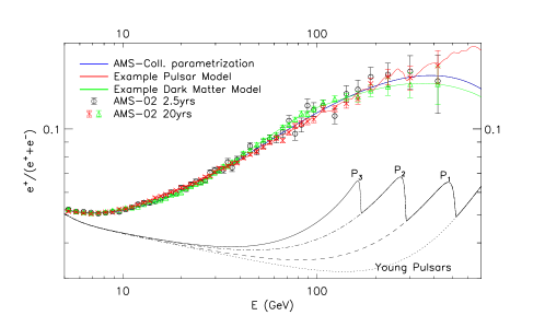
Figure 1: The AMS-02 positron fraction measurement Accardo et al. (2014) and two examples of models that fit it well. The red line is from the contribution of many Milky Way pulsars, while the green line is from a sample DM model. The DM spectrum is genuinely smooth, while the pulsar spectrum shows evidence of contributions from individual sources at high energies. The curves labeled P₁, P₂ and P₃, illustrate schematically the contribution from individual pulsars, at distances of 0.66, 0.97 and 1.7 kpc and ages of 240, 430 and 740 kyrs, respectively. The dotted line shows the contribution from pulsars with ages $\leq$150kyrs. We include a measurement of each model after 20yr with AMS-02. We would not be able to separate them through a fit to the spectrum. We include the AMS-Collaboration parametrization Accardo et al. (2014).

In this Letter, we suggest a power-spectrum technique to search for wiggles in the positron energy spectrum induced by discreteness of the source population. We perform 900 simulations of the Milky Way pulsar population accounting for the astrophysical uncertainties in this population. We then evaluate the prospects to detect, with this power-spectrum analysis, pulsar-induced wiggles. While current data are unlikely to have sufficient sensitivity, we find that the prospects to detect wiggles with forthcoming data are good enough to warrant a careful analysis.

Data: We use published AMS-02 data Accardo et al. (2014) that stem from 2.5 years of measurements from 5 GeV and up to 500 GeV. We also simulate for 20 yr assuming the same energy bins and percentage systematic errors. We also project three years of spectral measurements of the combined $e^{\pm}$ flux, up to 1 TeV, by DAMPE. In this letter we work with binned data, but note that there may be benefits, in a realistic analysis, to working with the raw data; especially if the bin widths exceed the instrumental resolution.

Pulsar-population uncertainties: The pulsars contribution to the local CR spectra, has several uncertainties. There are uncertainties on the neutron-star distribution in the Milky Way Faucher-Giguere and Kaspi (2006); Lorimer (2003); Lorimer et al. (2006) and their birth rate Dragicevich et al. (1999); Vranesevic et al. (2004); Faucher-Giguere and Kaspi (2006); Lorimer et al. (2006); Keane and Kramer (2008). For the spatial distribution we follow Ref. Lorimer et al. (2006), which relied on data from Ref. Manchester et al. (2001), and take a birth rate of 1/century. Details may be found in Appendix A. There are also uncertainties regarding the neutron stars’ initial spin-down power $\dot{E}_{0}$, braking index $\kappa$, and spin-down timescale $\tau_{0}$, that all relate to the time $t$-dependence of the spin-down power,

$$\dot{E}(t)=\dot{E_{0}}\bigg{(}1+\frac{t}{\tau_{0}}\bigg{)}^{-\frac{\kappa+1}{\kappa-1}}.$$ (1)

We assume that $\dot{E}_{0}$ follows a distribution $f(\dot{E}_{0})$, which we vary, in addition to varying $\kappa$ and $\tau_{0}$, ensuring that no pulsar has a spin-down power higher than the recorded ones Manchester et al. (2005); http://www.atnf.csiro.au/research/pulsar/psrcat , with details found in Appendix B.

Only a small fraction $\eta$, of the spin-down power can go to injected CR $e^{\pm}$ into the ISM. The CR $e^{\pm}$ before entering the ISM may be accelerated by the surrounding PWN and for younger pulsars the SNR shock front further out; this leads to significant uncertainties in the CR injection spectra. For each pulsar we assume a unique $\eta$ and energy spectrum $\frac{dN}{dE}_{e^{\pm}}\propto E^{-n}\,Exp\{-E/E_{\textrm{cut}}\}$, where $\eta$ and $n$ are described by equivalent distributions (i.e. no two pulsars in our simulations have identical $\eta$ or $n$). We test different variations on these distributions (details found in Appendix C). Finally as CR $e^{\pm}$ enter the ISM, they must propagate to the Earth where they are observed. There are uncertainties regarding the CR diffusion, energy-losses and the impact of the time-evolving Heliosphere. We have different assumptions to model the propagation through the ISM, using Malyshev et al. (2009); Cholis et al. (2016), while we account for the uncertainties of the propagation inside the Heliosphere (i.e. Solar Modulation Gleeson and Axford (1968)) by marginalizing over them following Cholis et al. (2016) and Cholis et al. (2017). For the time-evolution of the heliospheric magnetic field we use information from Ref. http://www.srl.caltech.edu/ACE/ASC/ ; http://wso.stanford.edu/Tilts.html (relevant details in Appendix D).

Given a spatial distribution and pulsar birth rate, a distribution $f(\dot{E}_{0})$, choices for $\kappa$ and $\tau_{0}$, distributions on the fraction of spin-down power that goes into ISM CR $e^{\pm}$ $g(\eta)$, distribution $h(n)$ on the injection index $n$, and choice of ISM propagation models, we generate a population of Milky Way pulsars that are within 4 kpc. To understand the impact of these uncertainties on the prospects to detect fluctuations in the positron energy spectrum, we produce 900 astrophysical realizations. Each one has a unique combination of the above ingredients while still consistent with pulsar population studies Faucher-Giguere and Kaspi (2006) and data on CR propagation in the ISM and the Heliosphere Trotta et al. (2011).

Technique: We fit the pulsar contribution to the AMS-02 positron-fraction (containing 51 data points between 5 and 500 GeV) by allowing for an additional normalization on the $e^{\pm}$ pulsar flux and by marginalizing over the uncertainties of primary and secondary CRs and Solar Modulation (leading to five fitting parameters). That alone constrains a significant fraction of the pulsar astrophysical realizations, if they are to explain the positron fraction. We leave that discussion for subsequent work Cholis et al. (2018). Of the 900 pulsar astrophysical realizations, only 172 fit the positron fraction within $3\sigma$ from a prediction of 1 per degree of freedom i.e. with a total $\chi^{2}\leq$ 64.2 for 51-5=46 d.o.f. . For the remainder of this analysis, we use those pulsar astrophysical realizations, one of which is shown in Fig. 1. Our results are not sensitive to the exact threshold that we place on the $\chi^{2}$ of the fit.

For each of the remaining 172 pulsar astrophysical realizations, we generate 10 observational realizations (i.e. add noise following the binning and errors of Ref. Accardo et al. (2014)); this can generate artificial fluctuations that mask the wiggles we seek. We then subtract from each observational realization the smoothed spectrum and evaluate the power-spectral density (PSD) of the residual spectrum. Since we do not know the true underlying astrophysical spectrum, we calculate for each realization the smoothed spectrum by convolving with a gaussian whose width increases with energy. This removes power in large scales in energy (low modes in the power spectrum) including contributions from instrument systematics as misestimates of the instrument efficiency or CR contamination. Yet, systematic artifacts in a small number of energy bins could still induce smaller-scale fluctuations that we seek.

To evaluate the PSD on the residual positron spectrum, we take the “time” parameter to be $ln(E/\textrm{GeV})$ which we assume to be measured in equal intervals. This is to a very good approximation true in the energy range 5–150 GeV, with higher energies having energy bins at larger separations. In our calculations we assume a logarithmic energy binning of $ln(E_{i}/\textrm{GeV})\equiv x_{i}=x_{0}+a\cdot i$, with $x_{0}=1.6571$ (5.24 GeV) and $a=0.063$. When comparing to current data, we go up to $i=59$ (215 GeV) while in our 20-year forecast we go up to $i=65$ (315 GeV). We calculate the PSDs for each of the 172$\times$10 observational realizations. Given the noise, there is scatter on the PSDs of the 10 observational realizations coming from the same underlying astrophysical realization.

To model the effect of observational scatter on the PSD, we use the AMS-02 smooth parametrization that fits well the data after 2.5 years and then produce 200 observational realizations of it. We then calculate the 200 PSDs on the residual. Those 200 observational realizations of the AMS-02 smooth parametrization provide the scatter on the PSD due to noise. For every one of the 60 (66) modes for the current (20 yr) data, we rank the 200 coefficients. We do not expect any correlations between modes. We use the 68$\%$ ranges to derive the $1\sigma$ error-bars per mode. We then determine a $\chi^{2}$ fit on each of the PSDs. Among the 200 observational realizations of the AMS-02 smooth parametrization there is a median in terms of its $\chi^{2}$ and $68\%$, $95\%$ and $99\%$ ranges. We use these ranges to compare the PSDs from physical models (pulsars or DM) and the PSD from noise. These ranges provide a measure of the scatter due to noise and whether pulsars can give a PSD signal above the noise.

Results: In the left panel of Fig. 2 we show the PSD of the measured AMS-02 positron fraction from the AMS-02 smooth parametrization (black line). The PSD of the noise realization with the median fit is given by the blue line. We also show the PSDs for the pulsar astrophysical realization and the DM model of Fig. 1 adding noise (red and green lines, respectively). As seen there, pulsars produce small-scale (small in $ln(E/\textrm{GeV})$) variations that lead to extra power in the PSD at high modes (large $f=1/ln(E/\textrm{GeV})$). The exact DM phenomenology (i.e mass annihilation/decay channel) can only affect the lower modes. DM models with one very evident and sharp spectral feature that could add some power are already excluded in Ref. Bergstrom et al. (2013); Ibarra et al. (2014). The difference between the red and the green PSDs on the residual positron fraction is what we are interested in. With 20 years of data the situation improves, as shown in the right panel of Fig. 2, for a 10$\%$ chance to see these fluctuations if pulsars are responsible for high-energy CR positrons.

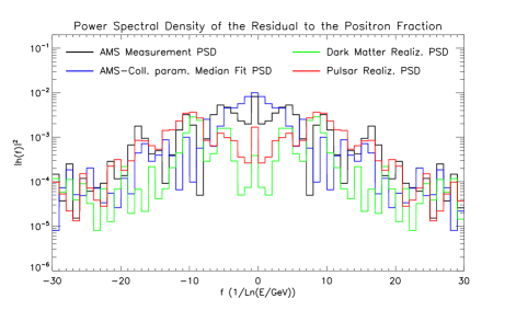
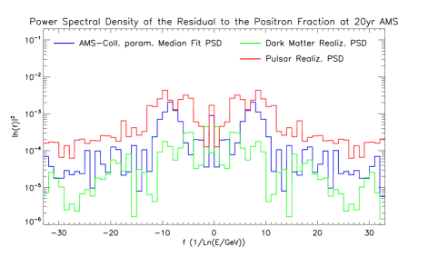
Figure 2: The PSD of the residual to the positron fraction from AMS-02. Left: current state with the black line giving the measurement, the blue line the noise realization with median fit and the red and green lines a pulsars and a DM realization. Since pulsars have spectral features (shown in Fig. 1), there is more power at the high modes of the PSD compared to the smooth DM realization. Right: Same after 20 yr of AMS-02 observations. The red line is calculated from one pulsar realization that is among the $\sim$10$\%$ of all our observation realizations, which give a signal in the PSD detectable at $\geq 2\sigma$.

In Fig. 3 we show for all 172 pulsar astrophysical realizations and for each of the 10 observational realizations the PSD $\chi^{2}$-distribution (red diamonds along y-axis). Each pulsar astrophysical realization is in a different position on the $x$-axis; ranked starting with the model that fits best the positron fraction spectrum. Our calculation of the fit of the observed AMS-02 PSD on the residual positron fraction is given by the black line. All diamonds, and the black line are to be compared to the three blue bands that represent the $68\%$, $95\%$ and $99.7\%$ ranges of the noise. We find that with current data 1.5$\%$ (12.5$\%$) of the 172$\times 10$ observation realizations lie outside the $99.7\%$ ($95\%$) band (left panel of Figure 3). This information is also given in Table 1. Since we have ranked our astrophysical realization models on the $x$-axis by their fit to the positron fraction, Fig. 3 also shows that there is no clear correlation between models that provide a poor fit to the smoothed energy spectrum and models that provide a poor fit to the power-spectrum. Also since the data PSD sits well within the 68$\%$ band of the noise, there is no indication yet that there is a deviation from a smooth spectrum; however, this null result cannot yet distinguish between different scenarios.

Figure 3: The scatter of 10 observational realizations in the PSD $\chi^{2}$/dof for each of the 172 pulsar astrophysical realizations (red diamonds). The blue bands include the noise ranges for the PSD $\chi^{2}$. Left: Current, with the black line giving the PSD of the measurement, showing no evidence for features. Right: After 20 years of data, $\sim 10\%$ of the pulsar realizations will provide (at 2$\sigma$) detectable fluctuations.

After 20 years of observations, and using information on the positron spectrum up to 315 GeV, the situation becomes more promising. Then, about 2.5$\%$ (10$\%$) of the observational realizations sit within the $99.7\%$ ($95\%$) noise bands, as shown in the right panel of Fig. 3 and in Table 1, with further details found in Appendix E.

Experiment	E-range	$\#$frq.	$\%$exc. f.	$\%$exc. f.	$\%$exc. f.
	(GeV)	modes	(95$\%$)	(99$\%$)	(99.7$\%$)
AMS-02 (2.5 yr)	5.2-215	$\pm 30$	12.5	3.5	1.5
AMS-02 (20 yr)	5.2-315	$\pm 33$	10	6	2.5
DAMPE (3 yr)	25-640	$\pm 19$	12	7	4

Table 1: The potential to observe power from small-scale features to the residual positron fraction (for AMS-02) or $e^{+}+e^{-}$ flux (for DAMPE). We give the relevant energy range to be used, the $\#$ of modes ($\pm$ 1/2 the number of logarithmically spaced E-bins). " $\%$exc. f." gives the $\%$ of realizations that fall outside the 95$\%$, 99$\%$ and 99.7$\%$ noise ranges.

DAMPE Chang et al. (2017); Ambrosi et al. (2017) and CALET Adriani et al. (2015, 2017) are now measuring the total CR $e^{+}+e^{-}$ flux up to several TeV. We forecast the prospects to probe a PSD signal from pulsars to higher energies where fewer pulsars contribute to the signal. Using the expected flux measurement between 25 and 640 GeV we find that 38 logarithmically equally spaced energy bins provides us with a good sensitivity to the presence of features. Of the 172 pulsars realizations, 53 include at least one pulsar that has similar power, age and distance as Geminga (PSR B0633+17) and one with similar properties for Monogem (PSR B0656+14). We use that subset, since these pulsars are relevant for that range of energies but not for the energy ranges used for the AMS-02 data. Our findings are given in Table 1 suggesting that indeed going to higher energies is necessary.

Discussion and Conclusions: In this Letter, we have proposed a power-spectrum analysis to identify wiggles in the positron energy spectrum that may arise from discreteness in the pulsar source population, in the event that pulsars are responsible for high-energy CR positrons. Our basic conclusions are that although such wiggles are likely too small to be detectable with current data, the prospects to see such wiggles with forthcoming data warrant the effort such an analysis would entail.

Our estimates of the detectability of the signal rely on a variety of uncertain ingredients in the modeling of the pulsar-population. To obtain some indication of these uncertainties, we constructed 900 simulated pulsar-population realizations each obtained with different assumptions about the neutron-star distribution, spin-down power characteristics and time-evolution, the injected CR $e^{\pm}$ spectra, and propagation through the ISM and the heliosphere, but requiring consistency with all observational constraints in each simulation used in the analysis. Thus, while our forecast of a $\sim$10$\%$ chance to detect these wiggles is uncertain, it is, we believe, based on realistic models. The takeaway message is therefore that the possibility to see something in a PSD analysis is significant enough to warrant a search. It is not, however, certain enough to ascribe any strong conclusions to a null result. With better understanding of the astrophysics in the next decade, the forecast may become more, or less optimistic, but almost certainly more robust. This analysis can be repeated for SNR sources.

The predictions of wiggles are statistical only. We ascribe significance to the presence of wiggles, but we do not make predictions about specific features at specific energies . We also do not ascribe the signal to any specific pulsar (e.g., Geminga or Monogem), although our models are required to have pulsar-populations consistent with the existence of these pulsars. Also, we emphasize that we simply estimate the sensitivity of current measurements to a power-spectrum-based wiggle search. We do hope, however, that this work motivates collaborations like AMS-02 and at higher energies DAMPE and CALET to perform their own PSD analysis with their data.

We thank Mirko Boezio, Joseph Gelfand, Ely Kovetz, Dmitry Malyshev, and Christoph Weniger for valuable discussions. This work was supported by NASA Grant No. NNX17AK38G, NSF Grant No. 0244990, and the Simons Foundation. This research project was conducted using computational resources at the Maryland Advanced Research Computing Center (MARCC).

Appendix A The Neutron Star Distribution in Space and Time

Ref. Lorimer et al. (2006) suggests that pulsars are born in the Milky Way at a rate of $1.4\pm 0.2$ pulsars per century Lorimer et al. (2006), although one finds a wider range of estimates in other work Dragicevich et al. (1999); Vranesevic et al. (2004); Faucher-Giguere and Kaspi (2006); Keane and Kramer (2008). For simplicity we assume a pulsar birth rate of one per century.

The spatial distribution of pulsars in the Galaxy has been investigated in Ref. Faucher-Giguere and Kaspi (2006); Lorimer (2003); Lorimer et al. (2006) relying on data from the Parkes multi-beam pulsar survey at 1.4 GHz Manchester et al. (2001). Our radial distribution of pulsars is based on the best-fit parameters of Ref. Lorimer et al. (2006), given by an empirical expression for the pulsar surface (column) density in the Galaxy,

$$\rho(R)=A(R/R_{\odot})^{B}\mbox{exp}\left(-C\frac{R-R_{\odot}}{R_{\odot}}\right)\mbox{ kpc}^{-2},$$ (2)

where $R$ is the Galactocentric radius and $R_{\odot}=8.5$ kpc is the distance of the Sun from Galactic center (GC). We use the values $B=1.9$ and $C=5.0$ given therein, normalizing $A$ such that we obtain our assumed birth rate. Our spatial simulations are consistent with Ref. Lorimer (2003) as shown in Fig. 4.

Using Eq. (2), we are lead to the following probability distribution function for the radial distance of a pulsar from GC,

$$PDF(R,B,C)=\frac{C^{B+2}}{Ae^{C}R_{\odot}^{2}}\frac{\rho(R)R}{\Gamma(B+2)},$$ (3)

where $\Gamma(x)$ is a Gamma function. We utilize a Laplace $z$-distribution with a characteristic scale of 50 pc as done in Ref. Faucher-Giguere and Kaspi (2006) and a flat angular distribution and simulate the pulsars within 4 kpc of the Sun.

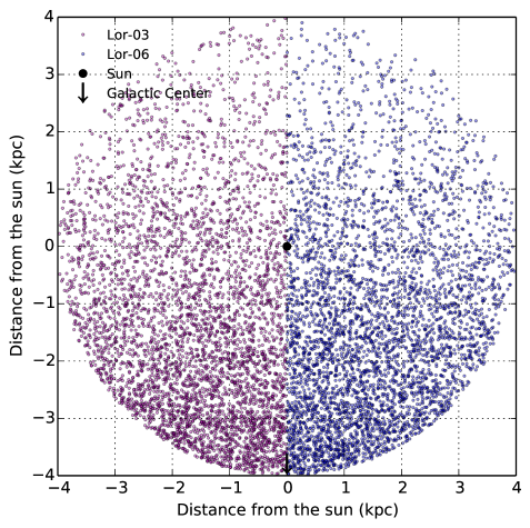
Figure 4: The pulsars simulated within 4 kpc of the Sun, projected onto the Galactic disk. The Galactic center is at $(0,-8.5)$ kpc. The Sun is the black dot at $(0,0)$. The magenta dots were simulated using the empirical pulsar radial distribution curve presented in Ref. Lorimer (2003). The blue dots were simulated using the best-fit pulsar radial distribution curve given in Ref. Lorimer et al. (2006). Both produce very similar results. The number of pulsars in both simulations were normalized such that one per century is born in the Galaxy, showing pulsars up to 10 Myr in age.

Appendix B The Neutron Stars Spin-Down Distribution Properties

Pulsar spin-down powers $\dot{E}$ are calculated using their ages and,

$$\dot{E}(t)=\dot{E_{0}}\bigg{(}1+\frac{t}{\tau_{0}}\bigg{)}^{-\frac{\kappa+1}{\kappa-1}}.$$ (4)

The spin-down timescale $\tau_{0}$ and the braking index $\kappa$ are varied per set of simulations. We let $\dot{E}_{0}=10^{x}$ ergs/s with $x=x_{\textrm{cutoff}}-y$ and where $y$ is taken from a log-normal distribution. The log-normal distribution is generated using the parameters $y_{\mu}$ and $y_{\sigma}$, which are the mean and standard deviation of the underlying Gaussian distribution. We consider four different values of $y_{\sigma}=[0.25,0.36,0.5,0.75]$. Values of $x_{\textrm{cutoff}}$ and $y_{\mu}$ are then chosen such that the distributions of observed pulse periods and surface magnetic fields of simulated pulsars are consistent with results presented in Fig. 6 of Ref. Faucher-Giguere and Kaspi (2006).

Finally, to ensure that we do not produce pulsars more luminous than the ones recorded in the ATNF catalog Manchester et al. (2005); http://www.atnf.csiro.au/research/pulsar/psrcat , we only consider values of $x<x_{\textrm{max}}=38.7$. In Table 2 we give all the spin-down power distribution properties for our pulsar simulations.

Sim no.	$\tau_{0}$ (kyr)	$\kappa$	$x_{\textrm{cutoff}}$	$y_{\mu}$	$y_{\sigma}$
30-59	$3.3$	$3$	$38.8$	$0.25$	$0.5$
120-149	$6$	$3$	$38.8$	$0.25$	$0.5$
150-179	$3.3$	$3$	$38.8$	$0.25$	$0.5$
180-209	$10$	$3$	$38.8$	$0.25$	$0.5$
210-239	$3.3$	$3$	$39$	$0.1$	$0.5$
240-269	$1$	$2.5$	$38.8$	$0.25$	$0.5$
270-299	$20$	$3.5$	$39$	$0.1$	$0.5$
300-329	$0.7$	$2.5$	$38.8$	$0.25$	$0.5$
330-359	$20$	$3.5$	$39.1$	$0.0$	$0.25$
360-389	$0.6$	$2.5$	$39.0$	$0.1$	$0.25$
390-419	$6$	$3$	$39.0$	$0.1$	$0.25$
420-449	$6$	$3$	$38.7$	$0.5$	$0.75$
450-479	$30$	$3.5$	$38.8$	$0.25$	$0.5$
480-509	$0.85$	$2.5$	$38.5$	$0.6$	$0.75$
510-539	$18$	$3.5$	$39.0$	$0.0$	$0.75$
540-569	$10$	$3$	$38.7$	$0.5$	$0.75$
570-599	$4$	$3$	$39.0$	$0.0$	$0.36$
600-629	$1$	$2.5$	$38.7$	$0.5$	$0.75$
630-659	$9$	$3$	$38.2$	$0.4$	$0.36$
660-689	$0.8$	$2.5$	$38.2$	$0.4$	$0.36$
690-719	$0.6$	$2.5$	$38.2$	$0.4$	$0.36$
720-749	$30$	$3.5$	$38.2$	$0.4$	$0.36$
750-779	$7$	$3$	$39.0$	$0.1$	$0.75$
780-809	$30$	$3.5$	$38.0$	$0.5$	$0.36$
810-839	$30$	$3.5$	$38.7$	$0.5$	$0.75$
840-869	$6$	$3$	$38.9$	$0.18$	$0.36$
870-899	$4.5$	$3$	$39.3$	$0.0$	$0.25$
900-929	$9$	$3$	$38.5$	$0.5$	$0.25$
930-959	$27$	$3.5$	$38.5$	$0.3$	$0.25$
960-989	$33$	$3.5$	$38.0$	$0.5$	$0.25$
990-1019	$0.85$	$2.5$	$38.3$	$0.5$	$0.25$

Table 2: The assumed pulsar-simulation spin-down power distributions and time evolution. Simulations $\#30-59$ are produced based on Ref. Lorimer (2003), while all others are on reference assumption of Ref. Lorimer et al. (2006).

Appendix C The Acceleration of CR electrons and positrons from Pulsars and Injection into the ISM

Electrons get accelerated inside the magnetosphere, produce ICS $\gamma$-rays, which in turn in the presence of strong magnetic fields pair produce $e^{\pm}$. These $e^{\pm}$ get further accelerated inside the magnetosphere. In addition, electrons and positrons will then propagate outwards losing energy during adiabatic E-losses, but can also be accelerated in the termination shock of the pulsar(also of the SNR) and the ISM. There is also evidence for $\gamma$-rays towards Geminga and Monogem Abdo et al. (2009); Abeysekara et al. (2017a, b), suggesting the presence of CR $e^{\pm}$ at 100 TeV in energy, losing a significant fraction of their energy within $\simeq 10$pc. Since the spin-down power drops with a time-scale of $\tau_{0}\mathrel{\raise 1.29167pt\hbox{$<$\kern-7.5pt\lower 4.30554pt\hbox{$\sim$}}}10^{4}$ yrs, about half of the rotational energy will be lost before the SNR shock front stops being an efficient accelerator and well before the PWN stops having an effect on these CRs. Given that the time for CR $e^{\pm}$ to propagate to Earth is an order of magnitude larger than $\tau_{0}$ we can consider their injection to the ISM instantaneous (see Ref. Malyshev et al. (2009) for further details).

In this work we are agnostic about the fraction $\eta$ of the spin-down power that goes into injected $e^{\pm}$. We assume a log-normal distribution for the $\eta$ parameter,

$$g(\eta)=\frac{Exp\left\{-\frac{\left[-\mu+ln(-1+\eta)\right]^{2}}{2\sigma^{2}}\right\}}{\sqrt{2\pi}(\eta-1)\sigma},$$ (5)

and take three different choices for $\mu$ and $\sigma$. These lead to three different choices for the combination of mean efficiency $\eta$, $\bar{\eta}=1+\textrm{Exp}\left\{\mu+\frac{\sigma^{2}}{2}\right\}$ and logarithmic standard deviation $\zeta=10^{\sigma}$: ($\bar{\eta}$, $\zeta$) = ($4\times 10^{-3}$, 1.47) or ($10^{-3}$, 2.85) or ($2\times 10^{-2}$, 1.29). As described in the main text, in fitting the positron fraction we allow for each astrophysical pulsar realization an overall normalization change in the pulsar component, that is absorbed into the specific values of $\bar{\eta}$. Our typical $\bar{\eta}$ is a few$\times 10^{-2}$ with a range of $2\times 10^{-3}-2\times 10^{-1}$.

For the injection CR $e^{\pm}$ spectra we assume,

$$\frac{dN}{dE}\propto E^{-n}Exp\left\{-\frac{E}{E_{\textrm{cut}}}\right\},$$ (6)

with $n$ following a flat distribution $g(n)$ either in a narrow range of $n\epsilon\left[1.6,1.7\right]$ or in a wider range of $n\epsilon\left[1.4,1.9\right]$. The upper cutoff $E_{\textrm{cut}}$ does not affect our fits to the observations, since the highest-energy CR $e^{\pm}$ quickly lose their energy before reaching us; we set it to $E_{\textrm{cut}}=10$ TeV.

Appendix D Cosmic-Ray Propagation through the ISM and heliosphere

From the moment CRs enter into the ISM they diffuse through the Milky Way magnetic field and suffer energy losses due to synchrotron radiation and inverse Compton scattering. We use five distinctive models for the ISM that agree with CR data including the B/C ratio, CR protons and He Cholis et al. (2016). The characteristics of these five ISM models are given in Table 3.

Model	$b$ ($\times 10^{-6}$GeV-1kyr-1)	$D_{0}$ (pc2/kyr)	$\delta$
A1	5.05	123.4	0.33
C1	5.05	92.1	0.40
C2	8.02	92.1	0.40
C3	2.97	92.1	0.40
E1	5.05	58.9	0.50

Table 3: The basic parameters that describe the propagations assumptions of cosmic rays in the Milky Way. Assuming isotropic and homogeneous diffusion, $D(R)=D_{0}(R/1GV)^{\delta}$. The energy losses due to synchrotron radiation and inverse Compton scattering are described by $dE/dt=-b\,E^{2}$.

The impact of these uncertainties on the morphology of the CR spectra is shown in Figure 5 for the positron fraction (colored lines). Depending on the assumptions on the energy losses and diffusion time-scales, the spectral features can be more pronounced or suppressed.

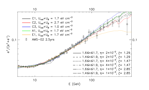
Figure 5: The positron fraction, assuming pulsars follow the same distribution in space and in their spin-down power and time evolution. We vary the ISM propagation conditions (different colors) as in Table 3, and the CR $e^{\pm}$ spectral properties and fraction of spin-down power into ISM injected $e^{\pm}$. $U_{\textrm{rad}}+U_{\textrm{B}}$ refer to the local energy density in the radiation and magnetic fields. Some of these lines are excluded in the positron fraction spectrum fit and are not used further in the PSD analysis.

Once exiting the ISM and entering the heliosphere, CRs will reach our detectors, after diffusing through the anisotropic magnetic-field structure of the fast evolving heliospheric magnetic field. During their propagation through the heliosphere, CRs also transfer via drift effects that impact how fast they will reach Earth, and the path they are most prone to follow through the Heliosphere. During that time CRs will also go through adiabatic energy losses. The effect of solar modulation on CR spectra is described by the solar-modulation potential $\Phi$ that describes the average energy losses CR suffer as they travel through the Heliosphere. That, in terms of CR spectra, is given by Gleeson and Axford (1968),

$$\frac{dN^{\oplus}}{dE_{kin}}(E_{kin}) = \frac{(E_{kin}+m)^{2}-m^{2}}{(E_{kin}+m+\mid Z\mid e\Phi)^{2}-m^{2}}$$ (7)

$$\times \;\frac{dN^{\rm ISM}}{dE_{kin}}(E_{kin}+\mid Z\mid e\Phi).$$

Here, $E_{kin}$ is the kinetic energy at Earth, and $\frac{dN^{\oplus(\textrm{ISM})}}{dE_{kin}}$ are the differential CR fluxes observed at Earth ($\oplus$) and the local interstellar medium (ISM) respectively. Finally, $\mid Z\mid e$ is the absolute charge of CRs.

Ref. Cholis et al. (2016), using proton fluxes from 1992 and up to 2010, resulted in the predictive, time-, charge- and rigidity(R)-dependent formula for the solar modulation potential,

$$\Phi(R,q,t)= \phi_{0} \,\bigg{(}\frac{|B_{\rm tot}(t)|}{4\,{\rm nT}}\bigg{)}+\phi_{1}\,H(-qA(t))\,\bigg{(}\frac{|B_{\rm tot}(t)|}{4\,{\rm nT}}\bigg{)}$$ (8)

$$\times \,\bigg{(}\frac{1+(R/R_{0})^{2}}{\beta(R/R_{0})^{3}}\bigg{)}\,\bigg{(}\frac{\alpha(t)}{\pi/2}\bigg{)}^{4},$$

with $R_{0}$ set to 0.5 GV and with a $2\sigma$ range for $\phi_{0}$ of 0.32–0.38 GV and $\phi_{1}$ in the range of 0–16 GV. We marginalize over these ranges of $\phi_{0}$ and $\phi_{1}$. In Eq. 8 we use the values of $B_{\rm tot}(t)$ and $\alpha(t)$ measured by ACE http://www.srl.caltech.edu/ACE/ASC/ and modeled in WSO http://wso.stanford.edu/Tilts.html . Having these values, we can directly calculate the $\Phi(R,q,t)$, for any CR species at a given rigidity and time t. For further details see Cholis et al. (2016).

Appendix E Pulsar Models Realizations versus Noise for AMS-02

In this appendix we provide additional information on how that observation realizations of the pulsar models that we test perform versus the expected noise of AMS-02 after 20 years of measurements.

In Figure 6 we plot the fraction of observation realizations of the pulsar models $f_{p}$ with a $\chi^{2}$/d.o.f larger than $f$, vs $f$ where $f$ is the fraction of smooth parameterization realizations.

Figure 6: The fraction of pulsar models observation realizations with $\chi^{2}$/d.o.f that is higher than the fraction $f$ of the smooth parameterization realizations, as a function of $f$ (x-axis). The blue diagonal line gives the case where $f_{p}=f$.

References

- Moskalenko et al. (2002) I. V. Moskalenko, A. W. Strong, J. F. Ormes, and M. S. Potgieter, Astrophys. J. 565, 280 (2002), eprint astro-ph/0106567.
- Kachelriess et al. (2015) M. Kachelriess, I. V. Moskalenko, and S. S. Ostapchenko, Astrophys. J. 803, 54 (2015), eprint 1502.04158.
- (3) http://galprop.stanford.edu/.
- Strong (2015) A. W. Strong (2015), eprint 1507.05020.
- Evoli et al. (2008) C. Evoli, D. Gaggero, D. Grasso, and L. Maccione, JCAP 0810, 018 (2008), eprint 0807.4730.
- (6) http://dragon.hepforge.org.
- Evoli et al. (2012a) C. Evoli, I. Cholis, D. Grasso, L. Maccione, and P. Ullio, Phys. Rev. D85, 123511 (2012a), eprint 1108.0664.
- Pato et al. (2010) M. Pato, D. Hooper, and M. Simet, JCAP 1006, 022 (2010), eprint 1002.3341.
- Di Bernardo et al. (2011) G. Di Bernardo, C. Evoli, D. Gaggero, D. Grasso, L. Maccione, et al., Astropart.Phys. 34, 528 (2011), eprint 1010.0174.
- Blasi (2009) P. Blasi, Phys. Rev. Lett. 103, 051104 (2009), eprint 0903.2794.
- Mertsch and Sarkar (2009) P. Mertsch and S. Sarkar, Phys. Rev. Lett. 103, 081104 (2009), eprint 0905.3152.
- Ahlers et al. (2009) M. Ahlers, P. Mertsch, and S. Sarkar, Phys. Rev. D80, 123017 (2009), eprint 0909.4060.
- Blasi and Serpico (2009) P. Blasi and P. D. Serpico, Phys.Rev.Lett. 103, 081103 (2009), eprint 0904.0871.
- Kawanaka et al. (2011) N. Kawanaka, K. Ioka, Y. Ohira, and K. Kashiyama, Astrophys. J. 729, 93 (2011), eprint 1009.1142.
- Fujita et al. (2009) Y. Fujita, K. Kohri, R. Yamazaki, and K. Ioka, Phys. Rev. D80, 063003 (2009), eprint 0903.5298.
- Cholis and Hooper (2014) I. Cholis and D. Hooper, Phys. Rev. D89, 043013 (2014), eprint 1312.2952.
- Mertsch and Sarkar (2014) P. Mertsch and S. Sarkar, Phys. Rev. D90, 061301 (2014), eprint 1402.0855.
- Di Mauro et al. (2014) M. Di Mauro, F. Donato, N. Fornengo, R. Lineros, and A. Vittino, JCAP 1404, 006 (2014), eprint 1402.0321.
- Kohri et al. (2016) K. Kohri, K. Ioka, Y. Fujita, and R. Yamazaki, PTEP 2016, 021E01 (2016), eprint 1505.01236.
- Harding and Ramaty (1987) A. K. Harding and R. Ramaty, International Cosmic Ray Conference 2, 92 (1987).
- Atoyan et al. (1995) A. M. Atoyan, F. A. Aharonian, and H. J. Völk, Phys. Rev. D 52, 3265 (1995).
- Aharonian et al. (1995) F. A. Aharonian, A. M. Atoyan, and H. J. Voelk, Astron. Astrophys. 294, L41 (1995).
- Hooper et al. (2009) D. Hooper, P. Blasi, and P. D. Serpico, JCAP 0901, 025 (2009), eprint 0810.1527.
- Yuksel et al. (2009) H. Yuksel, M. D. Kistler, and T. Stanev, Phys. Rev. Lett. 103, 051101 (2009), eprint 0810.2784.
- Profumo (2011) S. Profumo, Central Eur. J. Phys. 10, 1 (2011), eprint 0812.4457.
- Malyshev et al. (2009) D. Malyshev, I. Cholis, and J. Gelfand, Phys. Rev. D80, 063005 (2009), eprint 0903.1310.
- Kawanaka et al. (2010) N. Kawanaka, K. Ioka, and M. M. Nojiri, Astrophys. J. 710, 958 (2010), eprint 0903.3782.
- Grasso et al. (2009) D. Grasso et al. (Fermi-LAT), Astropart. Phys. 32, 140 (2009), eprint 0905.0636.
- Linden and Profumo (2013) T. Linden and S. Profumo, Astrophys.J. 772, 18 (2013), eprint 1304.1791.
- Cholis and Hooper (2013) I. Cholis and D. Hooper, Phys. Rev. D88, 023013 (2013), eprint 1304.1840.
- Yuan et al. (2015) Q. Yuan, X.-J. Bi, G.-M. Chen, Y.-Q. Guo, S.-J. Lin, and X. Zhang, Astropart. Phys. 60, 1 (2015), eprint 1304.1482.
- Yin et al. (2013) P.-F. Yin, Z.-H. Yu, Q. Yuan, and X.-J. Bi, Phys. Rev. D88, 023001 (2013), eprint 1304.4128.
- Bergstrom et al. (2008) L. Bergstrom, T. Bringmann, and J. Edsjo, Phys. Rev. D78, 103520 (2008), eprint 0808.3725.
- Cirelli and Strumia (2008) M. Cirelli and A. Strumia, PoS IDM2008, 089 (2008), eprint 0808.3867.
- Cholis et al. (2009a) I. Cholis, L. Goodenough, D. Hooper, M. Simet, and N. Weiner, Phys. Rev. D80, 123511 (2009a), eprint 0809.1683.
- Cirelli et al. (2009) M. Cirelli, M. Kadastik, M. Raidal, and A. Strumia, Nucl. Phys. B813, 1 (2009), [Addendum: Nucl. Phys.B873,530(2013)], eprint 0809.2409.
- Nelson and Spitzer (2010) A. E. Nelson and C. Spitzer, JHEP 10, 066 (2010), eprint 0810.5167.
- Arkani-Hamed et al. (2009) N. Arkani-Hamed, D. P. Finkbeiner, T. R. Slatyer, and N. Weiner, Phys. Rev. D79, 015014 (2009), eprint 0810.0713.
- Cholis et al. (2009b) I. Cholis, D. P. Finkbeiner, L. Goodenough, and N. Weiner, JCAP 0912, 007 (2009b), eprint 0810.5344.
- Cholis et al. (2009c) I. Cholis, G. Dobler, D. P. Finkbeiner, L. Goodenough, and N. Weiner, Phys. Rev. D80, 123518 (2009c), eprint 0811.3641.
- Harnik and Kribs (2009) R. Harnik and G. D. Kribs, Phys. Rev. D79, 095007 (2009), eprint 0810.5557.
- Fox and Poppitz (2009) P. J. Fox and E. Poppitz, Phys. Rev. D79, 083528 (2009), eprint 0811.0399.
- Pospelov and Ritz (2009) M. Pospelov and A. Ritz, Phys. Lett. B671, 391 (2009), eprint 0810.1502.
- March-Russell and West (2009) J. D. March-Russell and S. M. West, Phys. Lett. B676, 133 (2009), eprint 0812.0559.
- Chang and Goodenough (2011) S. Chang and L. Goodenough, Phys. Rev. D84, 023524 (2011), eprint 1105.3976.
- Dienes et al. (2013) K. R. Dienes, J. Kumar, and B. Thomas, Phys. Rev. D88, 103509 (2013), eprint 1306.2959.
- Finkbeiner and Weiner (2007) D. P. Finkbeiner and N. Weiner, Phys. Rev. D76, 083519 (2007), eprint astro-ph/0702587.
- Kopp (2013) J. Kopp, Phys. Rev. D88, 076013 (2013), eprint 1304.1184.
- Dev et al. (2014) P. S. B. Dev, D. K. Ghosh, N. Okada, and I. Saha, Phys. Rev. D89, 095001 (2014), eprint 1307.6204.
- Cholis et al. (2017) I. Cholis, D. Hooper, and T. Linden, Phys. Rev. D95, 123007 (2017), eprint 1701.04406.
- Tomassetti and Oliva (2017) N. Tomassetti and A. Oliva, Astrophys. J. 844, L26 (2017), eprint 1707.06915.
- Slatyer et al. (2009) T. R. Slatyer, N. Padmanabhan, and D. P. Finkbeiner, Phys. Rev. D80, 043526 (2009), eprint 0906.1197.
- Evoli et al. (2012b) C. Evoli, M. Valdes, A. Ferrara, and N. Yoshida, Mon. Not. Roy. Astron. Soc. 422, 420 (2012b).
- Madhavacheril et al. (2014) M. S. Madhavacheril, N. Sehgal, and T. R. Slatyer, Phys. Rev. D89, 103508 (2014), eprint 1310.3815.
- Ade et al. (2016) P. A. R. Ade et al. (Planck), Astron. Astrophys. 594, A13 (2016), eprint 1502.01589.
- Slatyer (2016) T. R. Slatyer, Phys. Rev. D93, 023527 (2016), eprint 1506.03811.
- Poulin et al. (2016) V. Poulin, P. D. Serpico, and J. Lesgourgues, JCAP 1608, 036 (2016), eprint 1606.02073.
- Tavakoli et al. (2014) M. Tavakoli, I. Cholis, C. Evoli, and P. Ullio, JCAP 1401, 017 (2014), eprint 1308.4135.
- Geringer-Sameth et al. (2015) A. Geringer-Sameth, S. M. Koushiappas, and M. G. Walker, Phys. Rev. D91, 083535 (2015), eprint 1410.2242.
- Ackermann et al. (2015) M. Ackermann et al. (Fermi-LAT), Phys. Rev. Lett. 115, 231301 (2015), eprint 1503.02641.
- Abeysekara et al. (2017a) A. U. Abeysekara et al., Astrophys. J. 843, 40 (2017a), eprint 1702.02992.
- Abeysekara et al. (2017b) A. U. Abeysekara et al. (HAWC), Science 358, 911 (2017b), eprint 1711.06223.
- Abdo et al. (2009) A. A. Abdo et al., Astrophys. J. 700, L127 (2009), [Erratum: Astrophys. J.703,L185(2009)], eprint 0904.1018.
- Hooper et al. (2017a) D. Hooper, I. Cholis, T. Linden, and K. Fang, JCAP (2017a), [Phys. Rev.D96,103013(2017)], eprint 1702.08436.
- Linden et al. (2017) T. Linden, K. Auchettl, J. Bramante, I. Cholis, K. Fang, D. Hooper, T. Karwal, and S. W. Li, Submitted to: Phys. Rev. D (2017), eprint 1703.09704.
- Abramowski et al. (2016) A. Abramowski et al. (H.E.S.S.), Nature 531, 476 (2016), eprint 1603.07730.
- Hooper et al. (2017b) D. Hooper, I. Cholis, and T. Linden (2017b), eprint 1705.09293.
- Dragicevich et al. (1999) P. M. Dragicevich, D. G. Blair, and R. R. Burman, Mon. Not. R. Astron. Soc. 302, 693 (1999).
- Vranesevic et al. (2004) N. Vranesevic et al., Astrophys. J. 617, L139 (2004), eprint astro-ph/0310201.
- Faucher-Giguere and Kaspi (2006) C.-A. Faucher-Giguere and V. M. Kaspi, Astrophys. J. 643, 332 (2006), eprint astro-ph/0512585.
- Lorimer et al. (2006) D. R. Lorimer et al., Mon. Not. Roy. Astron. Soc. 372, 777 (2006), eprint astro-ph/0607640.
- Keane and Kramer (2008) E. F. Keane and M. Kramer, Mon. Not. Roy. Astron. Soc. 391, 2009 (2008), eprint 0810.1512.
- Cholis and Weiner (2009) I. Cholis and N. Weiner (2009), eprint 0911.4954.
- Cholis et al. (2009d) I. Cholis, L. Goodenough, and N. Weiner, Phys. Rev. D79, 123505 (2009d), eprint 0802.2922.
- Accardo et al. (2014) L. Accardo et al. (AMS), Phys. Rev. Lett. 113, 121101 (2014).
- Lorimer (2003) D. R. Lorimer (2003), [IAU Symp.218,105(2004)], eprint astro-ph/0308501.
- Manchester et al. (2001) R. N. Manchester et al., Mon. Not. Roy. Astron. Soc. 328, 17 (2001), eprint astro-ph/0106522.
- Manchester et al. (2005) R. N. Manchester, G. B. Hobbs, A. Teoh, and M. Hobbs, Astron. J. 129, 1993 (2005), eprint astro-ph/0412641.
- (79) http://www.atnf.csiro.au/research/pulsar/psrcat.
- Cholis et al. (2016) I. Cholis, D. Hooper, and T. Linden, Phys. Rev. D93, 043016 (2016), eprint 1511.01507.
- Gleeson and Axford (1968) L. J. Gleeson and W. I. Axford, Astrophys. J. 154, 1011 (1968).
- (82) http://www.srl.caltech.edu/ACE/ASC/.
- (83) http://wso.stanford.edu/Tilts.html.
- Trotta et al. (2011) R. Trotta, G. Johannesson, I. V. Moskalenko, T. A. Porter, R. R. de Austri, and A. W. Strong, Astrophys. J. 729, 106 (2011), eprint 1011.0037.
- Cholis et al. (2018) I. Cholis, T. Karwal, and M. Kamionkowski (2018), eprint 1807.05230.
- Bergstrom et al. (2013) L. Bergstrom, T. Bringmann, I. Cholis, D. Hooper, and C. Weniger, Phys.Rev.Lett. 111, 171101 (2013), eprint 1306.3983.
- Ibarra et al. (2014) A. Ibarra, A. S. Lamperstorfer, and J. Silk, Phys. Rev. D89, 063539 (2014), eprint 1309.2570.
- Chang et al. (2017) J. Chang et al. (DAMPE), Astropart. Phys. 95, 6 (2017), eprint 1706.08453.
- Ambrosi et al. (2017) G. Ambrosi et al. (DAMPE) (2017), eprint 1711.10981.
- Adriani et al. (2015) O. Adriani, Y. Akaike, K. Asano, Y. Asaoka, M. G. Bagliesi, G. Bigongiari, W. R. Binns, S. Bonechi, M. Bongi, J. H. Buckley, et al., in Journal of Physics Conference Series (2015), vol. 632 of Journal of Physics Conference Series, p. 012023.
- Adriani et al. (2017) O. Adriani et al. (CALET), Phys. Rev. Lett. 119, 181101 (2017), eprint 1712.01711.