Symmetry protected bosonic topological phase transitions: Quantum Anomalous Hall system of weakly interacting
spinor bosons in a square lattice
Fadi Sun1,2,4, Junsen Wang 1,3, Jinwu Ye 1,2,4, Shaui Chen 3 and Youjin Deng 31 Department of Physics and Astronomy, Mississippi State University, MS, 39762, USA
2 Department of Physics, Capital Normal University,
Key Laboratory of Terahertz Optoelectronics, Ministry of Education, and Beijing Advanced innovation Center for Imaging Technology,
Beijing, 100048, China
3 CAS Center for Excellence and Synergetic Innovation Center in Quantum Information and Quantum Physics,
University of Science and Technology of China, Hefei, Anhui 230026, China
4 Kavli Institute of Theoretical Physics, University of California, Santa Barbara, Santa Barbara, CA 93106
Abstract
We study possible many body phenomena in the Quantum Anomalous Hall system of weakly interacting spinor bosons in a square lattice.
There are various novel spin-bond correlated superfluids (SF) and quantum or topological phase transitions among these SF phases.
One transition is a first order one driven by roton droppings ( but with non-zero gaps ) tuned by the Zeeman field .
Another is a second order bosonic Lifshitz transition with the dynamic exponents and
an accompanying symmetry breaking. It is
driven by the softening of the superfluid Goldstone mode tuned by the ratio of
spin-orbit coupled (SOC) strength over the hopping strength.
The two phase boundaries meet at a topological tri-critical (TT) point which separates the line into two SF phases
with and condensation momenta respectively.
At the line where the system has an anti-unitary Reflection symmetry, there are infinite number of
classically degenerate family of states on both sides. We perform a systematic order from quantum disorder analysis to find the
quantum ground states, also calculate the roton gaps generated by the order from disorder mechanism on both sides of the TT point. The and SF phases have the same spin-orbital XY-AFM spin structure, respect the anti-unitary symmetry
and break the symmetry, so they be distinguished only by
the different topology of the BEC condensation momenta instead of by any differences in the symmetry breaking patterns.
This could be a first bosonic analog of the fermionic topological Lifshitz transition with the change of the topology of
the Fermi surfaces, Dirac points or Weyl points.
However, when moving away from line, the Reflection symmetry is lost, the TT is converted to
the second order bosonic Lifshitz transition.
All these novel quantum or topological phenomena can be probed in the recent experimentally realized weakly
interacting Quantum Anomalous Hall (QAH) model of by Wu, et.al, Science 354, 83-88 (2016).
The investigation and control of spin-orbit coupling (SOC) have become
subjects of intensive research in both condensed matter and cold atom systems after the discovery
of the topological insulators kane ; zhang .
In materials side,
the Rashba SOC plays crucial roles in various 2d or layered insulators, semi-conductor systems, metals and superconductors without inversion symmetry.
The Quantum Anomalous Hall ( QAH ) effect was experimentally realized
in Cr doped Bi(Sb)2Te3 thin films QAHthe ; QAHexp and also observed in many other materials such as both Cr doped and V doped (Bi,Sb)2Te3 films. In the cold atom side,
using Raman scheme, one experimental group expk40 ; expk40zeeman generated 2d Rashba SOC
for gas. Using the optical Raman lattice scheme,
the bosonic analog of the QAH for spinor bosons 87Rb was realized in 2dsocbec .
It was known that one serious shortcoming for using Raman scheme to generate SOC in alkali fermions,
is the strong heating associated with spontaneous emissions.
The heating issue hindered the observation of true many body phenomena for alkali fermions.
So the physics observed in expk40 ; expk40zeeman is still
at single particle physics. However, the heating issue is much less serious for spinor boson 87Rb atoms in the weakly interacting regime.
Indeed, the lifetime of SOC 87Rb BEC was already made as long as in 2dsocbec and improved to
recently more , so the current experiment set-up the stage to observe any possible many body phenomena at a weak interaction
where the heating rate is well under current experimental control.
More recently, optical lattice clock schemes SD ; clock have been successfully implemented clock1 ; clock2 to generate 1d SOC for and . This newly developed scheme has the advantage to suppress
the heating issue suffered in the Raman scheme.
It can also be used to probe the interplay between the interactions and the SOC easily.
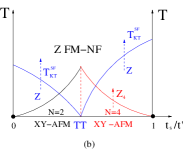
Figure 1: The global phase and phase transitions as a function of and .
In the yellow region, the mean field state is the Z FM-SF with only one minimum located at .
In the blue region, the mean field state is the Z FM-SF with only one minimum located at .
Both states keep the symmetry, so are non-degenerate.
In the green regime, the mean field state is the Z-XY FM-SF with four minima located at
where depends on . It breaks , so is 4 fold degenerate.
There is a first order quantum phase transition at driven by the roton dropping tuned by
the Zeeman field. There is a second order quantum bosonic Lifshitz phase transition with the dynamic exponents
driven by the softening of the SF Goldstone mode tuned by the ratio across the phase boundary.
The two phase transition boundaries meet at the Topological Tri-critical (TT) point at which separates
the XY-AFM state from the XY-AFM state.
Their boson condensation functions are given by Eq.12 and Eq.30,32 respectively.
Both states have the same XY-AFM spin-orbital structure, respect the anti-unitary symmetry and
break the symmetry, so they can be distinguished only by
the different topology of the BEC condensation momenta in Fig.2 instead of by any differences in the symmetry breaking patterns.
The ground state at the left Abelian point is a FM SF in the basis,
That at the right Abelian point is a frustrated SF with the coplanar spin-orbital structure in the basis.
For the finite temperature phase transitions above all the SF phases, see Fig.8,9.
However, so far the experiment2dsocbec is still at single particle level: namely mapping of the topological
band of the QAH model Eq.1
using the thermally excited 87Rb atoms, no study of quantum many body phenomena yet.
The ultimate goal of the experiments in 2dsocbec is to study many body phenomena of SOC 87Rb BEC.
This directly motivated us to investigate possible many-body phenomena of the QAH model of the spinor bosons Eq.1
at a weak interaction.
We find the competition among the hopping, the SOC and the Zeeman field in the QAH model Eq.1 leads to
a hopping dominated ( Abelian ) regime and a SOC dominated ( non-Abelian ) regime in the phase diagram of Fig.1.
While the upper part with the Zeeman field is related to the lower part by a anti-unitary Reflection transformation Eq.2. There are
various novel spin-bond correlated superfluid states and also new classes of quantum or topological phase transitions among these SF phases.
One transition is a first order one driven by roton droppings ( but with non-vanishing roton gaps )
at tuned by the Zeeman field .
Another is a second order one driven by the softening of the superfluid Goldstone mode tuned by the ratio of
SOC strength over the hopping strength. It is a bosonic Lifshitz transition with the dynamic exponents
and an accompanying symmetry breaking.
The two phase boundaries meet at the topological tri-critical ( TT ) point which separates the line into two SF phases
with and condensation momenta respectively.
At , the system has the Reflection symmetry,
there are classically degenerate family of states with the dimension and manifold in the two sides respectively.
We perform a novel systematic order from quantum disorder analysis to find true quantum ground states
and also calculate the roton gaps generated by the order from disorder mechanism on both sides of the TT point.
The two SF phases have the same spin-orbital XY-AFM spin-orbital structure with degeneracy,
respect the anti-unitary symmetry
and break the identical other symmetries of the Hamiltonian. So they can not be distinguished
by any difference in the symmetry breakings
except by the different topology of the BEC condensation momenta.
This could be a first bosonic analog of the fermionic topological Lifshitz transition
of free fermions with Fermi surfaces, Dirac points or Weyl points topo1 ; topo2 .
However, when moving away from line, the Reflection symmetry is lost, the TT is converted to
the second order bosonic Lifshitz transition with the accompanying symmetry breaking.
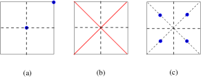
Figure 2: The reflection symmetry protected TPT at . (a) The SF at the left has BEC condensation momenta
at and .
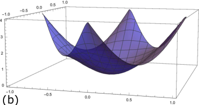
(b) At the TPT, the dispersion becomes flat along the two crossing lines .
(c) The SF at the right has BEC condensation momenta at .
Both SF phase have the same XY-AFM spin-orbital structure with
degeneracy naive .
The results achieved in this work can be detected in the ongoing experiment 2dsocbec ; more ,
especially the topological phase transition at the TT can be directly detected by the Time of flight (TOF) imaging.
They may guide and inspire the ongoing world wide experimental efforts expk40 ; expk40zeeman ; SD ; clock ; clock1 ; clock2 to
study new many body phenomena due to the interplay between SOC and interactions.
Surprisingly, so far, there is very little work to study the effects of interaction on QAH in the materials side either,
so our results and methods may also shed some lights on studying interaction effects on QAH materials QAHthe ; QAHexp .
The experimentally realized Quantum Anomalous Hall ( QAH ) model of spinor bosons in a square lattice
is described by the Hamiltonian:
(1)
where the spinor could be either fermions or bosons.
For 87Rb atoms, the two pseudo-spin components
denote the two hyperfine states or .
In this paper, we focus on the spin isotropic interaction which may also be the
most experimentally relevant one.
In addition to the particle number symmetry,
the Hamiltonian has a symmetry. At , there is an enlarged anti-unitary Reflection symmetry:
(2)
where (1) A spin rotation leads to ;
(2) A time reversal leads to ;
(3) A sublattice rotation leads to .
Under , .
So there is an enlarged symmetry at .
RESULTS
1. Mean field Analysis of the ground states in space.
In the weak interaction limit which is also the most experimentally easily accessible limit,
One can first diagonals the non-interacting the bosonic QAH Hamiltonian Eq.1 and locate the minima positions
shown in Fig.1 which has 3 different regimes shown in Fig.1.
(a) When and , there is only one minimum located at with the
spinor spin up, called Z FM-SF. It respects the symmetry.
(b) When and , there is only one minimum located at
with the spinor spin down, called Z FM-SF. It also respects the symmetry.
(c) When ,
there are four minima:
, ,
, and ,
where ;
the corresponding spinors are
(3)
where and
(4)
In the limit ( namely, close to the right Abelian axis ), the phase boundary diverges,
it means there is no phase transition on the right axis in Fig.1. Indeed, as , , , so only in the limit , indicating no phase transition on the right axis.
This is in sharp contrast to the strong coupling limit where it was established
there is a quantum phase transition at a finite Zeeman field rhht .
The most general single-particle ground state can be written as:
(5)
where the four coefficients are normalized .
Its interaction energy can be written in terms of . When ,
its minimization shows the mean field ground state is always a plane wave state where the interaction energy simplifies to
. The spin of the plane wave state at is along
which has both Z component and a component in XY plane oriented at , so named
Z-XY FM-SF. It breaks the symmetry.
As , then , , so the spin lies in the XY plane.
As approaches the upper ( or lower ) boundary, ( or ),
, so the spin aligns along the spin up ( or spin down ) direction, so the Z-XY FM-SF reduces to the
Z FM-SF ( or Z FM-SF ) respectively.
At the Tri-critical point T at , the minima become
the two crossing lines .
When , these mean field states are labeled as Z FM-SF, Z FM-SF and Z-XY FM-SF
in the phase diagram Fig.1. In the following sections, we will treat as a weak interaction to study the excitations above all the phases.
However, at , there are classically degenerate family of states,
so mean field can not determine the true quantum ground state.
In Sec.3 and 5, we will perform the Order from quantum disorder analysis to determine the true ground state
from the degenerate family of classical states at , then calculate the excitation spectrum.
We will also investigate quantum or topological phase transitions among all these phases.
2. The excitation spectrum in the Z FM-SF at .
When the spectrum minimum is located at or , the non-interacting Hamiltonian takes a simple form
(6)
where the SOC drops out.
Let us consider case, thus the minimum is located at .
In the weak coupling limit , by writing
(7)
where is the number of condensate atoms,
and is the total number of lattice sites, thus is the condensate fraction.
We can perform the expansion where the superscript denotes the order in the quantum fluctuations.
The zeroth order term is the classical energy of the condensate.
The vanishing of the linear term sets the value of the chemical potential .
Diagonizing by a generalized Bogliubov transformation leads to:
(8)
where . are the two Bogliubov modes.
Since always holds, so we focus on
which displays a gapless superfluid Goldstone mode near and
a gapped roton mode at . In the long wavelength limit, we find
the superfluid Goldstone mode becomes linear where the velocity is
(9)
which is shown in Fig.3a. In limit, it reduces to .
How the SF Goldstone mode and the gapped roton mode behave as one approaches
the phase boundaries in Fig.1 is shown in Fig.3.
(a). The second order bosonic Lifshitz transition from the Z FM to the Z-XY FM
For a general , it is easy to see that the velocity of the SF Goldstone mode Eq.9
vanishes as one approaches the phase boundary ( Fig.3a ) where the dispersion becomes quadratic:
(10)
which shows the transition from the Z FM to the Z-XY FM is a bosonic Lifshitz transition with the dynamic
exponents . The equality of is dictated by the symmetry in the Z FM SF
with either spin up or spin down in Fig.1 z2 .
There is an accompanying transition in the spin sector from the Z FM to the Z-XY FM with the symmetry breaking
pattern .
The Bosonic Lifshitz transition from commensurate canted phase to non-coplanar IC-SkX with the anisotropic dynamic exponents was studied in rhh .
In Fig.3a, at a fixed , as increases to sitting on the
boundary between Z FM-SF and
the Z-XY FM-SF at , the slope of the Goldstone mode at decreases as in Eq.9,
then becomes quadratic at the boundary as shown in Eq.10.
(b). The first order transition from the Z FM-SF to the Z FM-SF driven by the roton dropping.
In Fig.3b, at a fixed , as increases to sitting on the boundary between Z FM-SF at and
the Z FM-SF at , the roton mode gets lower and lower,
then touches zero at .
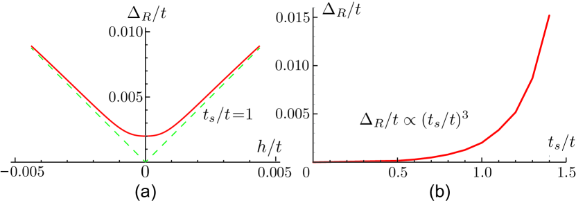
In the small limit, we find the roton gap which is independent of
( the dashed line in Fig.6a ).
Naively, this behaviour may signify a possible second order transition.
However, as to be shown in the next section, the order from quantum disorder analysis show that
the quantum fluctuations will open a roton gap at ( the real line in Fig.6a ).
So the roton driven transition is a first order one.
(c). The TT point approaching from the left.
The above two phase transition boundaries meet at the Topological Tri-critical (TT)
point where
(11)
which becomes flat along the two crossing lines shown in Fig.2b.
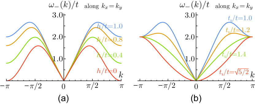
Figure 3:
The Critical Behaviour of the superfluid Goldstone mode starting at .
(a) Decreasing from 1 to 0, the roton at gets lower and lower and drops to zero at
signifying a first order transition.
(b) Increasing from to its critical value , the SF Goldstone mode gets softer and softer
and becomes quadratic at the phase boundary signifying a second order bosonic transition.
We used .
3. The Order from disorder phenomena and the XY-AFM state at .
At the two minima and , the term vanishes, so the effects of SOC do not show up at the mean field level.
They only show up at quantum fluctuations. At ( or ), the minimum is at ( or ),
it is these quantum fluctuations which lead to the gapless Goldstone mode
and the gapped roton mode discussed in the above section.
At , in the left of the T point in Fig.1,
the two minima become degenerate, there is a classically degenerate family of ground states:
(12)
where and are any two complex numbers satisfying the normalization condition
. The ”quantum order from disorder” mechanism is needed to determine that the quantum ground state
in this family of the classical degenerate ground state.
We write the spinor field as the condensation part Eq.12 plus a quantum fluctuating part
. Again, the zero order term gives the classical ground state
energy .
Setting the linear term vanish gives the value of the chemical potential .
Diagonizing by a generalized Bogliubov transformation leads to:
(13)
where the RBZ has the diamond shape and
with are the four Bogoliubov modes and the
ground-state energy incorporating the quantum fluctuations is
(14)
where .
After parameterizing and as
(15)
We find the minima of is located at
and (See also Fig.5 ). So the “order from disorder” mechanism
picks up the 4-fold degenerate state in Eq.12 as the quantum ground states whose associated
spin-orbit structure is:
(16)
which is a AFM state in the XY plane. Obviously, it breaks the with fold degeneracy.
After identifying the correct quantum ground-state as the XY-AFM state,
we can also evaluate all in Eq.13.
There are one linear SF Goldstone mode and
one quadratic roton mode located at shown in Fig.4.
Figure 4: (a) There is a linear SF Goldstone mode at .
(b) There is also a quadratic roton mode at .
The roton mode will acquire a gap due to the order from disorder mechanism as shown in Fig.6.
and are fully gapped higher energy modes, so not shown.
We used and .
(a) The Roton mass gap generated from the ”order by disorder” mechanism in the XY-AFM state
The ”order from disorder” mechanism picks up and as the quantum ground state.
Then we can expand the ground-state energy around the minimum as:
(17)
where and , the two coefficients and
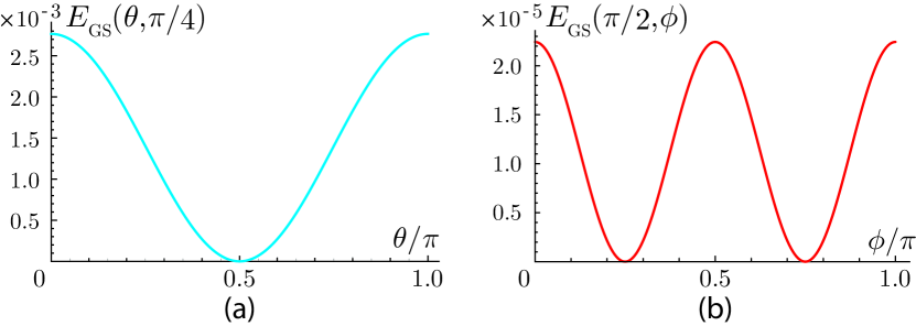
can be extracted from Fig.5.
Figure 5: The quantum ground-state energy near its minimum at
(a) at fixed , (b) at fixed
where the coefficients and in Eq.17 can be extracted respectively.
We used and .
Using the commutation relations , one can see that
the ”quantum order from dis-order ” mechanism generates the roton gap:
(18)
which is shown in the Fig.6.
The SF Goldstone mode remains unaffected. This is consistent with its protection by the symmetry breaking.
In fact, the symmetry at dictates without fixing the relative phase.
So the XY-AFM states still keep the symmetry.
The transition at is a first order phase transition driven by the roton dropping tuned by the Zeeman field .
But the roton still has a non-zero gap before it sparks the first order transition as shown in Fig.6.
The XY-AFM state is a pure state instead of a mixed state of the spin up state and spin down state
with any ratio. This is in sharp contrast to the 1st order transition between the Y-x state and X-y state in Ref.rhrashba .
However, as to be shown in Fig.8, it may melt into such a mixed state through a finite temperature
clock transition.
Figure 6: (a)Roton gap computed
by the order from disorder analysis as a function of zeeman field at a given .
Other parameters are , .
The dashed line of the roton dropping is before the order from disorder calculations.
(b) At , the Roton gap computed by the order from disorder analysis
is an increasing function of as approaching to the T point from the left.
Other parameters are , .
At , it is nothing but the FM spin wave mode.
At small , it can also be calculated by the perturbation theory in
which leads to ( see Method ).
Compare with on the right side in Fig.7.
4. The excitation spectrum in the Z-XY FM SF at .
AS shown in Sec.1, the ground state is just a plane wave (PW) state.
Without a loss of generality, we choose the PW state at the momentum .
From Eq.3, we can rewrite spinor field as:
(19)
Following the similar procedures as in section 2,
Setting the Linear term vanishing determines the chemical potential where
.
We also reach the form of Eq.8 where
.
We found one Goldstone mode at ,
which, in the long wavelength limit, takes the form
(20)
where and take the analytic form:
(21)
(22)
(a). The second order bosonic Lifshitz transition from the Z-XY FM to the Z FM
It is easy to see that both velocities vanish in the phase boundary in Fig.1 where the dispersion
becomes quadratic which is identical to that listed in Eq.10.
This agreement between approaching the boundary from the left and
from the right shows that the transition is indeed a second order bosonic Lifshitz
transition with the dynamic exponent and also the accompanying symmetry breaking in the spin sector.
(b). The first order transition between the two Z-XY FM states driven by the roton dropping.
In the limit, , the Goldstone mode becomes
(23)
where .
We also found that there are 3 gapped rotons near , , and .
In the limit, ,
The two rotons
near and
start to touch down and also become two linear modes ( the upper dashed line in Fig.7a ):
(24)
While the roton near also starts to touch down, but become quadratic
( the lower dashed line in Fig.7a ):
(25)
where
(26)
It is easy to see the three linear modes and
are , but the quadratic mode still exists even in the limit
where it becomes identical to the free particle mode. This is clearly an arti-fact of the calculations
at this order. In the following, we will show that the order from disorder analysis will open gaps
to and . So the transition is a first order one.
(c). The TT point approaching from the right.
If approaching the TT point from the right, taking
in Eq.23, then which becomes flat along the line .
Of course, if we choose the PW state at the momentum in Eq.19,
then which becomes flat along the line .
So the two flat directions from the left in Eq.11 are just the combination of the one near and
another one near .
5. The Order from disorder phenomena and the XY-AFM at .
We will study the nature of SF phase in the SOC dominated regime in Fig.1.
In sharp contrast to the hopping dominated regime discussed above, the SOC term shows its dominating
effects even at the mean field level.
But the effects of drops off at the mean field level.
There is a spurious symmetry at the 4 minima. The effects of only show up in the quantum fluctuations.
This is just opposite or dual to the hopping dominated regime in Sec.3 where the effects of dominates, while drops off
at the mean field level as discussed above.
At , in the right of the T point , , the four minima are located at
, ,
, and . The corresponding four spinors in Eq.3 become
(27)
The fact that the gapless mode at one momentum and
the simultaneous touching down of the three rotons at the other three momenta as indicates all the four momenta
maybe involved in the ground at . The most general mean field ground state can be written as:
(28)
where .
When evaluating its interaction energy,
the most salient feature here is that a loop term involving going around the 4 minima by one turn is a reciprocal lattice,
so this Umklapp process is crucial even at the mean field level which is absent
when where evaluated below Eq.5.
Here the interaction energy takes a rather symmetric form:
(29)
where the complex number .
Its minimization leads to .
By counting the number of free real parameters,
one can see the dimension of classically degenerate family ground state manifold is .
In fact, as to be explained in the next subsection, in addition to the exact symmetry,
the Hamiltonian has a spurious symmetry. So it counts as .
So the ”quantum order from disorder” mechanism is needed to determine the quantum ground state
from the degenerate family Eq.28.
At the right Abelian point, the spin symmetry becomes exact, but the remains spurious.
Our previous work on the right Abelian point absf showed that
the order from disorder mechanism on the spurious classically degenerate family will pick up
a plane-wave state ( namely, one of the in Eq.27 )
plus its spin related family in limit.
For a small deviation from the Abelian limit, i.e. , the exact spin symmetry
becomes spurious at mean field level. So we expect the order from disorder mechanism will pick up
a true quantum ground state from this spin related family.
We did the order from disorder analysis in the three channels generated by the three
generators
which generate the orbital orders and respectively.
Due to the symmetry and channels are identical, so
one only need to focus on. The results are shown in Fig.11.
The details are given in the Method section where we find the quantum ground state happens in the
channel:
(30)
which corresponds to in Eq.28.
Its corresponding spin-orbit structure is:
(31)
which is only the or combinations in Eq.16,
so it only has the degeneracy rotation11 .
Equivalently, it can happen in the channel:
(32)
which corresponds to in Eq.28 with or
combinations in Eq.16. It only has the degeneracy.
When combining Eq.30 with Eq.32, it is a 4-fold degenerate state related by the symmetry.
Surprisingly, the combined spin-orbital structure of the two sets of Bose condensations is the same as that on the right Eq.16
with the same degeneracy .
Even so, the boson wavefunctions Eq.30 and Eq.32 on the right with condensation momenta
differ from Eq.12 with condensation momenta on the left rotation11 ,
so this must be a TPT which resembles the TPT in a fermionic system topo1 ; topo2 .
This could be the first bosonic analog of the fermionic topological Lifshitz transition
of free fermions with Fermi surfaces, Dirac points or Weyl points topo1 ; topo2 .
We also computed the
4 roton gaps generated from the ” quantum order from disorder ”
shown in Fig.7.
Figure 7: (a) The three roton gaps
computed from the order from disorder analysis
as a function of at a fixed . We used .
The dashed line is the roton dropping without the order from disorder analysis.
(b) All the three roton gaps are monotonically increasing functions of as approaching to
the TT point from the right at . We used .
Compare with on the left side in Fig.6.
The first order transition at is driven by the roton dropping at
with the gap .
are essentially irrelevant to the first order transition.
6. The physical picture near the left Abelian point and near the right Abelian point
At the left Abelian point , after the transformation ,
the spin symmetry becomes evident in the rotated basis .
This left Abelian point is controlled by the spin-conserved hopping term .
There is no coupling between the off-diagonal long range order
in the SF sector and the magnetic order in the spin order. The breaking of and that of spin
leads to the linear superfluid Goldstone mode and the quadratic FM spin wave mode respectively and separately.
When slightly away from the left Abelian point along the horizontal axis, a small SOC term will break the symmetry. However, at the minimum and , the term still drops out, so the SOC still plays no roles at the mean field level, however, it still plays important roles in the quantum fluctuations. So the exact symmetry becomes a spurious one, so an order from disorder
phenomena is needed to find the quantum ground state from the classically degenerate family of states Eq.12 due to this spurious symmetry. Indeed, as shown in the order from disorder analysis in the Sec.3, it is quantum fluctuations induced by the SOC term which picks up the XY AFM state as the quantum ground state, also open the gap to the roton mode shown in Fig.6.
At , the XY-AFM becomes a FM in the XY plane in the basis,
so the roton mode is nothing but the FM spin wave mode.
The term opens a gap to the FM spin wave mode and transfer it to a pseudo-Goldstone mode.
As shown in the method section, in the basis, the second order perturbation in picks up the XY plane,
the fourth order perturbation selects and the gap .
Transforming back to the original basis, it is the XY-AFM state.
So the result is consistent with the order from disorder analysis done in the original basis in Sec.3.
When slightly away from the left Abelian point along the vertical axis, the state is just the Z FM state, the Zeeman field simply opens a gap to
the FM spin wave mode and transfer it to a pseudo-Goldstone mode.
In the right Abelian point , the spin symmetry becomes evident
in the rotated basis
which was used in rh ; rhht ; rhh ,
This right Abelian point is controlled by the SOC term .
As shown in absf , there is a strong quantum fluctuations induced by the coupling between the off-diagonal long range order
in the SF sector and the magnetic order in the spin order ( This is in sharp contrast to
the physics at the left Abelian point discussed above where there is no such coupling.)
The complete symmetry breaking leads to
4 linear gapless modes. When transforming the Abelian gauge to the present non-abelian gauge with ,
the co-planar state becomes the XY-AFM state,
the 4 linear modes are shifted to the 4 minima .
When slightly away from the right Abelian point along the horizontal axis, a small term will break the symmetry.
However, the term still drops out at the 4 minima , it
still plays no roles at the mean field level.
So the exact spin symmetry becomes a spurious one, so an order from disorder
phenomena is needed to find the quantum ground state from the classically degenerate family of states Eq.28 due to this spurious symmetry. So we expect one gapless mode remains, the other three become gapped pseudo-Goldstone modes.
Indeed, as summarized in the order from disorder analysis in the Sec.5 and detailed in the method section, the small term
picks up the XY AFM state Eqs.30,32
as the quantum ground state, also open the gap to the two linear modes
at and to the quadratic mode
at . Of course, the linear gapless SF Goldstone
mode at remains due to the symmetry breaking.
When slightly away from the right Abelian point along the vertical axis, there should be two gapless Goldstone modes
one at due to breaking the , another at due to breaking the which is a subgroup
of . Indeed, taking the results on Z-XY state in Sec.4, as at ,
namely, approaching the right axis at , we find and all approach zero.
However, the order from disorder analysis at the right axis junsen opens the gap to the and channel.
While the gapless mode at is the just the Goldstone mode due to the breaking.
So all the quantum phase transitions in Fig.1 can be considered as the one from the phases
controlled by the conventional hopping ( Abelian regime ) to the phases
controlled by the SOC term ( Non-Abelian regime )
( Note that is the flux Abelian point.)
7. Finite Temperature Phase transitions.
Now we briefly discuss the finite temperature phases and phase transitions above all the SFs in Fig.1.
Of course, due to the symmetry breaking in the SF phase, there is always a KT transition above all the SFs.
Due to the correlated spin-bond orders of the SFs, there are also other phase transitions associated with the restorations of these
orders at finite temperatures shown in Fig.8 and Fig.9. The nature of these finite temperature transitions can be qualitatively determined by the degeneracy of the ground states:
Z FM-SF (spin up or down ) ( ), Z-XY FM-SF (spin up or down ) ( ), and XY-AFM ( )
which breaks not only the global symmetry, but also the spin-orbital symmetry.
Especially, at , there is a finite temperature clock transition from both the and
XY-AFM to a mixed state which is
a mixture of the phases at the two sides and at any ratios in Fig.8.
If the transition is the first order one driven by roton dropping tuned by the Zeeman field
as in Fig.8, the SF KT transition is higher near the transition.
If the transition is the second order bosonic Lifshitz one driven by the softening
of the SF Goldstone mode tuned by as in Fig.9, the SF KT transition is lower near the transition.
But the two finite phase transition lines could cross when away from the transition.
The gap above the XY-AFM in Fig.6b and above the XY-AFM in Fig.7b
directly determine the finite of the two clock transitions above the two XY-AFM states respectively in Fig.9b.
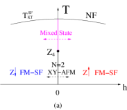
Figure 8: The finite temperature phase transitions at a given .
The 1st order quantum phase transitions at are driven by roton dropping tuned by the Zeeman field.
There is symmetry of finite .
(a) at a fixed . At , there is a finite temperature clock melting transition
with from the XY-AFM ( a pure state )
to a mixed state which consists of any mixture of spin up FM-SF at and spin down FM-SF at .
There is also a higher KT transition from the SF to a normal fluid (NF).
(b) at a fixed . There is also a clock transition above the
XY-AFM to destroy the XY component of the spin with .
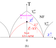
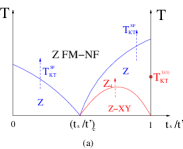
Figure 9: The finite temperature phase transitions at a given with .
(a) at a fixed .
The quantum phase transitions at is a Bosonic Lifshitz transition with the dynamic exponent
driven by the softening of superfluid Goldstone mode.
There are KT transitions at from the SF to a normal fluid (NF) on both sides.
There is lower clock melting transition to destroy the XY component of the spin on the right side .
On the right axis, there is also a KT transition due to the symmetry breaking in the basis.
(b) at a fixed .
The Topological Tri-critical (TT) point at .
There are clock transition with above the XY-AFM in Fig.6b and
above the XY-AFM in Fig.7b respectively.
The left and right dot stands for the the and symmetry respectively.
8. Implications on ongoing experimental efforts on QAH 87Rb atoms to detect the many body phenomena
In the ongoing experiment at USTC 2dsocbec , the BEC has atoms and trapped within the diameter ,
so one lattice site has about atoms.
The short-range Hubbard like interaction in Eq.1.
Plugging in the S-wave scattering length of the 87Rb atoms where is the Bohr radius
and the mass of the Spinor bosons 87Rb atoms lead to .
The interaction also has a negligible spin anisotropy with .
It is easy to evaluate the density-spin correlation functions whose poles should be determined by
the Bogliubov spectrum in Fig.3,4,6 with the corresponding spectral weight. So all interesting behaviors of the Goldstone mode near and the roton mode near in these figures can be precisely monitored and mapped out by the Bragg spectroscopies becbragg used in the same lab before. For example,
taking a point such as landing in the spin up FM SF in Fig.1,
Tuning to observe the roton softening by the Bragg spectroscopies becbragg is a easy task.
However approaching the bosonic Lifshitz transition boundary in Fig.1 is more challenging.
The hopping is determined by the depth of the optical lattice generated by a standing wave laser,
while the SOC is determined by the strength of the traveling Raman laser.
But the numerical value of the ratio was not estimated in the experiment2dsocbec , because it is not
important to the single particle band structure anyway which shows QAH as long as the SOC strength .
However, as shown in Fig.1, it is important in
the many body phenomena explored here. So increasing the depth of the optical lattice and also the strength of the Raman laser
should be able to increase the ratio to reach SOC dominated non-Abelian regime in Fig.1.
Then the novel many body phenomena of this non-Abelian regime can be experimentally detected.
The Time of Flight (TOF) image after a time is given by blochrmp :
(33)
where , is the form factor due to the
Wannier state of the lowest Bloch band of the optical lattice and
is the equal time boson structure factor.
For small condensate depletion in the weak coupling limit ,
where is the condensate wavefunction.
Obviously, the wavefunctions of the PW state leading to
Z FM-SF (spin up or down ) ( ), the PW state Eq.19 leading to the Z-XY FM-SF (spin up or down ) ( )
can be easily detected. At , due to the order from disorder mechanism,
both the XY-AFM boson wavefunction Eq.12 in the hopping dominated Abelian regime and
the XY-AFM boson wavefunctions Eq.30, Eq.32 in the SOC dominated non-Abelian regime lead to
the spin-orbital XY-AFM ( with the degeneracy ) in Eq.16.
The TOF can detect the differences in the BEC condensation topology
between the two bosonic wavefunctions which lead to the same set of spin-orbital structures.
So the TOF can detect all the quantum and topological phenomena in Fig.1.
The spin-orbital structures, the excitations above the SF phases across the whole BZ,
the transitions driven by the roton dropping or the softening of the SF Goldstone bosons and
the location of the TT point can be precisely determined by various experimental techniques
such as dynamic or elastic, energy or momentum resolved, longitudinal or
transverse Bragg spectroscopies becbragg ; bragg1 ; bragg2 ,
specific heat measurements heat1 ; heat2 and In-Situ measurements dosexp .
DISCUSSIONS
The TPT in non-interacting fermions can be characterized by the change in the topology of Fermi Surface (FS),
the Dirac point or Wely point topo1 ; topo2 where the low energy fermionic excitation stay.
Here, for bosonic SF system which is necessarily an interacting system, we propose to characterize the
TPT by the change in the topology of BEC condensation momenta where the low energy bosonic excitation stay.
The TPT is protected by a anti-unitary discrete symmetry which is the reflection symmetry in the present context.
Under the transformation, the momentum changes as
.
So the BEC condensation momenta in the left of Fig.2 transform to each other,
while the BEC condensation momenta in the right of Fig.2 are invariant under the transformation.
This is the only two possibilities which lead to the ground states with
the XY-AFM spin-orbital structure respecting the symmetry.
The ”order from quantum disorder” phenomena and the associated mass generations
have been studied in the geometrically frustrated magnets ringrev ; sachdev .
In this work, for the first time, we studied
the novel frustrated phenomena due to the SOC leading to QAH at zero Zeeman field in Fig.1.
Most interestingly, the quantum ground and XY-AFM state selected by the ”order from quantum disorder” phenomena
is a pure state instead of a mixed state of the two states at and .
This is in sharp contrast to the case in the Rashba SOC induced frustration in quantum spin systems rhrashba .
These studies in the SOC frustrated superfluids
should open new horizons to its original discovery in the context of frustrated magnetisms.
It was known that Haldane model haldane0 in a honeycomb lattice is the first QAH model.
Due to the two sublattice structure of the honeycomb lattice, it only needs Abelian gauge field.
The effects of interaction on the Haldane model in its spin-less or spinful version has been
investigated by various groups canada . However, to realize QAH in a square lattice, a non-abelian gauge field
( or SOC ) term in Eq.1 is needed. Surprisingly, the interaction effects of QAH model in a square lattice
has been completely overlooked so far. Obviously, due to its Non-Abelian nature,
the many body phenomena are quite different than those in the Haldane-Hubbard model.
If reversing the sign of the down hopping term in Eq.1, then it maps to the
isotropic Rashba model studied in Ref.rh ; rhrashba
with in a Zeeman field .
Of course, it is this sign difference which introduces the third Pauli spin even
at the zero Zeeman field and introduces topological band structure at a finite Zeeman field
in the QAH model. Therefore, the QAH model displays dramatically different many body phenomena
than the interacting Rashba or Weyl SOC systems rh ; rhht ; rhh ; rhrashba ; rasf .
So the two systems are complementary and shed lights to each other.
It was known that the Rashba SOC band structure does not have topological properties.
It remains interesting to explore how this (non)-topological band structure affects
the many body phenomena for spinor bosons at both weak and strong interaction.
Methods
1. Perturbation theory at a small to calculate the roton gap in the
XY-AFM phase in the hopping dominated Abelian regime.
In the left side of Fig.1, at small and , we perform the perturbation calculation
in which is independent, but complementary to the order from disorder analysis done in Sec.3.
We work in basis in Fig.1.
When evaluating the ground-state energy upto fourth order in , we determine the state
with and to be the round state, which, after transforming back
the original basis, is the XY-AFM state on the left in Fig.1.
We begin with an unperturbed Hamiltonian in the basis with no SOC ,
(34)
where
and . It is essentially a spinor boson Hubbard model.
Adding flux to this model leads to the Abelian point on the right in the basis absf .
Because it has the symmetry,
one can condense the spinor bosons at with the spin symmetry breaking direction
along . The can be diagonalized by a Bogoliubov transformation:
(35)
where is the Ferromagnetic (FM) spin mode
and
is the superfluid (SF) Goldstone mode which, in fact, is the same as that in a single component case.
In sharp contrast to the flux Abelian point in the right of Fig.1 where there is a coupling between the
density mode and spin mode absf , here the FM spin mode is decoupled from the SF density mode.
In the basis, one can write the SOC term as:
(36)
where .
Using the fact that the unperturbed ground-state is the vacuum of
and in Eq.35:
, One can just apply non-degenerate perturbation
theory in to calculate the corrections to the ground state energy.
Because , one can see that odd order corrections vanish, so
(37)
where
(38)
After some length, but straightforward manipulations, we find:
(39)
where . so reaches its minimum at leading to .
Unfortunately, is independent of , so one must work out upto the fourth order corrections.
After some length, but straightforward manipulations, we find that at fixed :
(40)
where . So reaches its minimum at leading to .
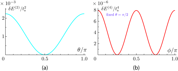
In Fig.10, we plot the numerical values of and
which match the numerical data from the direct calculations. Fig.10 is consistent with
Fig.5, so we reach the same ground state XY-AFM on the left side of Fig.1 from
two independent methods. From Eq.39 and 40, one can extract , so
Eq.18 leads to shown in Fig.6.
Figure 10: (a) The 2nd order correction to the ground-state energy
as a function of with fixed and .
(b) The 4th order correction to the ground-state energy
as a function of with fixed and .
In order to see the energy difference clear, we shifted all the energy by its minimum.
In principle, one can apply a similar perturbation theory near the right flux Abelian point in Fig.1 where .
In the basis,
one may treat as a small perturbation when slightly away from the flux Abelian point.
Unfortunately, in practice, due to the coupling between the SF mode and the spin mode already at the flux Abelian point,
the perturbation calculations are too complicated to extract useful information.
It seems the ” order from quantum disorder” analysis is the only
practical way to determine the true ground state and also calculate the spectrum which we do in the following.
2. Calculating the roton gaps in the XY-AFM phase in the SOC dominated Non-Abelian regime by order from disorder analysis
As shown in the section 6, the exact symmetry at the right Abelian point in the rotated basis becomes a
spurious one when away from it by . So order from disorder analysis is needed to calculate the roton gaps
at or and at in the XY-AFM phase.
(a). Estimations of .
The Spin-orbital rotation acting on the state
generates a superposition of condensations at and .
The most general state in such a superposition is:
(41)
where one may note that are not orthogonal as listed in Eq.27.
Of course, due to the symmetry, and work equally well
with in Eq.41. In the following, we will work in this sub-manifold to estimate the gap .
Using and , we can construct the two eigenstates of as
whose minimization leads to .
Indeed, setting in Eq.29 leads to which, in turn,
also leads to .
The order from quantum disorder analysis in Eq.41 selects ( Fig.11a )
which corresponds to the plane wave state or .
Expanding around the and
expanding the quantum fluctuations corrected quantum ground state energy around the saddle point at
in the Fig.11a leads to:
(46)
where is from the classical contribution in Eq.45 and
is from the quantum fluctuations which can be extracted from Fig.11a.
The commutation leads to the roton gap
at :
(47)
whose numerical values are shown in Fig.7.
The symmetry dictates .
Figure 11:
(a) The quantum fluctuations corrected ground state energy as a function of at
fixed and , and .
is the ground-state energy in the channel consisting of the condensations
at and in Eq.41.
is the ground-state energy in the channel consisting of the condensations
at and in Eq.48.
(b)
as a function of at a fixed .
In order to see the energy difference clear, we shifted all the energy by its minimum at .
(b). Calculations of
The Spin-orbital rotation acting on the state
generates a superposition of condensations at and .
The most general state in such a superposition is:
Its interaction energy is independent of both and .
Indeed, setting in Eq.29 automatically leads to which is independent of
and .
The order from quantum disorder analysis in Eq.48
selects and ( Fig.11 )
which corresponds to
leading to Eq.30
(or corresponding to
for and in Eq.48 leading to Eq.32. )
Expanding the quantum ground state energy around the minimum
in the Fig.11 leads to:
(52)
where and can be extracted
from Fig.11a and b respectively. Both come from the quantum fluctuations.
It is constructive to compare this equation with Eq.17 generating the roton gap in Fig.6 on the left side.
The commutation leads to the roton gap at :
(53)
which is shown in Fig.7 and smaller than by a factor .
Of course, the first order transition as is driven by the roton dropping at with the gap .
are essentially irrelevant to the first order transition.
(c). Most general analysis in the whole degenerate manifold.
In order to do a most general analysis, following similar order from disorder analysis
on the left side of Fig.1, we write the spinor field as the condensation part Eq.28
plus a quantum fluctuating part .
The zeroth order term is the classical energy of the condensate.
The vanishing of the linear term sets the value of the
chemical potential. Diagonizing by a generalized Bogliubov transformation leads to:
(54)
where is the RBZ.
The ground state energy incorporating the contributions from the quantum fluctuations is:
(55)
For general 5 dimension classic ground state manifold,
we know 1 dimension is come from the particle number conservation symmetry broken
and any state differ by a globe phase have the same energy.
We performed a grid search in the whole 4-dimension manifold
and confirmed that equal superposition of and ( or and )
condensation Eq.30 (or Eq.32 ) have the lowest energy,
therefore are the XY-AFM quantum ground state with the total degeneracy .
3. The kinetic energy and density current in all the phases in Fig.1
Using the method in yan , we will evaluate the conserved density current in all the phases, especially in the and
XY-AFM phases. In the context of 2d charge-vortex duality yan ,
the vortex currents in the dual lattice gives the boson densities in the direct lattice.
Here, it would be interesting to see if the two XY-AFM have different current distributions.
However, as shown in the following, the current turns out to be zero in all the phases.
This confirms further the and XY-AFM phase can not be distinguished by any symmetry breaking principles.
There is a TPT between the two phases.
We can write the kinetic energy in Eq.1 as
(56)
where .
Along a given bond :
(57)
where is the kinetic energy and is the current flowing along the bond yan .
For a genetic plane-wave state ,
(58)
In the following, we evaluate the kinetic energy and the
conserved density current in all the 4 phases respectively.
They can be directly measured by the In Situ experimental techniques.
By comparing the kinetic energies in the Eq.66 with Eq.68,
we can see that the lowest kinetic energy bond vanishes at the TT, then changes its sign.
This salient feature maybe related to the two crossing flat directions shown in Fig.2b.
Acknowledgements
We thank Bao Zhen, Wu Zan for helpful discussions.
F. Sun and J. Y acknowledge AFOSR FA9550-16-1-0412 for supports.
The work at KITP was supported by NSF PHY11-25915.
J.W and Y.D thank the support by NSFC under Grant No. 11625522 and the Ministry of Science and
Technology of China (under grants 2016YFA0301604).
References
(1)
M. Z. Hasan and C. L. Kane, Colloquium: Topological insulators, Rev. Mod. Phys. 82, 3045 (2010).
(2)
X. L. Qi and S. C. Zhang, Topological insulators and superconductors, Rev. Mod. Phys. 83, 1057 (2011).
(3) Rui Yu, Wei Zhang, Hai-Jun Zhang, Shou-Cheng Zhang, Xi Dai1, Zhong Fang,
Quantized Anomalous Hall Effect in Magnetic Topological Insulators, Science 329, 61 (2010).
(4) Cui-Zu Chang, Jinsong Zhang, Xiao Feng, Jie Shen, Zuocheng Zhang, Minghua Guo1, Kang Li, Yunbo Ou, Pang Wei, Li-Li Wang, Zhong-Qing Ji, Yang Feng1, Shuaihua Ji, Xi Chen, Jinfeng Jia1, Xi Dai2, Zhong Fang2, Shou-Cheng Zhang3, Ke He2,?, Yayu Wang1,?, Li Lu2, Xu-Cun Ma2, Qi-Kun Xue1, Experimental Observation of the Quantum Anomalous Hall Effect
in a Magnetic Topological Insulator, Science 340, 167 (2013).
(5) Lianghui Huang, et.al,
Experimental realization of a two-dimensional synthetic spin-orbit coupling in ultracold Fermi gases, Nature Physics 12, 540-544 (2016).
(6) Zengming Meng, et.al,
Experimental observation of topological band gap opening in ultracold Fermi gases with two-dimensional spin-orbit coupling, arXiv:1511.08492.
(7) Zhan Wu, Long Zhang, Wei Sun, Xiao-Tian Xu, Bao-Zong Wang, Si-Cong Ji, Youjin Deng, Shuai Chen, Xiong-Jun Liu, Jian-Wei Pan, Realization of Two-Dimensional Spin-orbit Coupling for Bose-Einstein Condensates, Science 354, 83-88 (2016).
(8) Zhan Wu, et.al, in progress.
(9) O. Boada, A. Celi, J. I. Latorre, and M. Lewenstein, Quantum Simulation of an Extra Dimension, Phys. Rev. Lett. 108, 133001 C Published 29 March 2012; Featured in Physics: Cultivating Extra Dimensions, Published 29 March 2012; A. Celi, P. Massignan, J. Ruseckas, N. Goldman, I.?B. Spielman, G. Juzeli nas, and M. Lewenstein, Synthetic Gauge Fields in Synthetic Dimensions, Phys. Rev. Lett. 112, 043001 C Published 28 January 2014.
(10) Michael L. Wall, et.al, Synthetic Spin-Orbit Coupling in an Optical Lattice Clock, Phys. Rev. Lett. 116, 035301 (2016).
(11)
L. F. Livi, G. Cappellini, M. Diem, L. Franchi, C. Clivati, M. Frittelli, F. Levi, D. Calonico, J. Catani, M. Inguscio, L. Fallani,
Synthetic dimensions and spin-orbit coupling with an optical clock transition, Phys. Rev. Lett. 117, 220401 C Published 23 November 2016.
Editors’ Suggestion.
(12)
S. Kolkowitz, S.L. Bromley, T. Bothwell, M.L. Wall, G.E. Marti, A.P. Koller, X. Zhang, A.M. Rey, J. Ye,
Spin-orbit coupled fermions in an optical lattice clock, arXiv:1608.03854. See also Jun Ye s talk at the
” Synthetic Quantum Matter” workshop at KITP, Nov.28,2016,
http://online.kitp.ucsb.edu/online/synquant16/ye/
(13)
Fangzhao Alex An, Eric J. Meier, Bryce Gadway, Direct observation of chiral currents and magnetic reflection in atomic flux lattices,
arXiv:1609.09467.
(14) Nathaniel Q. Burdick, Yijun Tang, and Benjamin L. Lev, Long-Lived Spin-Orbit-Coupled Degenerate Dipolar Fermi Gas,
Phys. Rev. X 6, 031022 C Published 17 August 2016.
(15) Naively, one may think the BEC condensation has the Rotation symmetry, while the
one does not. However, the symmetry of the Hamiltonian is instead of just the .
So the 4-fold XY-AFM and 4-fold XY-AFM transform exactly the same way under the transformation.
(16) Fadi Sun, Jinwu Ye, Wu-Ming Liu, Quantum magnetism of spinor bosons in optical lattices with synthetic non-Abelian gauge fields
at zero and finite temperatures, Phys. Rev. A 92, 043609 (2015).
(17) Fadi Sun, Jinwu Ye and Wu-Ming Liu, Classification of magnons in Rotated Ferromagnetic Heisenberg model and their competing responses in transverse fields, Phys. Rev. B 94, 024409 ( 2016 ).
(18) Fadi Sun, Jinwu Ye, Wu-Ming Liu, Quantum incommensurate Skyrmion crystal phases and Commensurate to In-commensurate transitions of cold atoms and materials with spin orbit couplings, New J. Phys. 19, 083015 (2017).
(19) Fadi Sun and Jinwu Ye,
In-commensurate Skyrmion crystals, devil staircases and multi-fractals due to spin orbit coupling in a lattice system, arXiv:1603.00451.
(20) Fadi Sun, Junsen Wang, Jinwu Ye and Youjin Deng, Novel superfluids of interacting spinor bosons in a Rashba spin-orbital coupled square lattice, Preprint
(21) Fadi Sun, Junsen Wang, Jinwu Ye and Youjin Deng, Frustrated superfluids of multi-component bosons in a flux on a square lattice, Preprint
(22) We did not write the dynamic exponent as , becasue Eq.10 only has a cubic symmetry instead of the emergent rotational symmetry.
(23) It can be shown that the bosonic wavefunctions Eq.30
differ from Eq.12 with by a position dependent phase and
a global spin rotation around the symmetry breaking axis along the direction.
Similarly, the bosonic wavefunctions Eq.32
differ from Eq.12 with by a position dependent phase and
a global spin rotation around the symmetry breaking axis along the direction.
(24)
Immanuel Bloch, Jean Dalibard, and Wilhelm Zwerger, Many-body physics with ultracold gases, Rev. Mod. Phys. 80, 885 (2008).
(25) Si-Cong Ji, Long Zhang, Xiao-Tian Xu, Zhan Wu, Youjin Deng, Shuai Chen, and Jian-Wei Pan, Softening of Roton and Phonon Modes in Bose-Einstein Condensate with Spin-Orbit Coupling, Phys. Rev. Lett. 114, 105301 C Published 9 March 2015,
(26) Jinwu Ye, J.M. Zhang, W.M. Liu, K.Y. Zhang, Yan Li, W.P. Zhang, Light scattering detection of various quantum phases of ultracold atoms in optical lattices, Phys. Rev. A 83, 051604 (R) (2011). See comments below.
(27) Jinwu Ye, K.Y. Zhang, Yan Li, Yan Chen and W.P. Zhang, Optical Bragg, atom Bragg and cavity QED detections of quantum phases and excitation spectra of ultracold atoms in bipartite and frustrated optical lattices,
Ann. Phys. 328 (2013), 103-138.
(28)
Kinast, J. et al.
Heat Capacity of a Strongly Interacting Fermi Gas.
Science307, 1296 (2005).
(29)
Ku, M. J. H. et al.
Revealing the Superfluid Lambda Transition in the Universal Thermodynamics of a Unitary Fermi Gas.
Science335, 563 (2012).
(30) Gemelke, N., Zhang X., Huang C. L., and Chin, C. In situ observation of incompressible Mott-insulating domains in ultracold atomic gases, Nature (London) 460, 995 (2009).
(31) Fa-Di Sun, Xiao-Lu Yu, Jinwu Ye, Heng Fan, W. M. Liu,
Topological Quantum Phase Transition in Synthetic Non- Abelian Gauge Potential:
Gauge Invariance and Experimental Detections, Scientific Reports 3, 2119 (2013).
(32) Fadi Sun and Jinwu Ye, Type I and Type II fermions, Topological depletions and sub-leading scalings across
topological phase transitions, Phys. Rev. B 96, 035113 (2017).
(33) Junsen Wang, Fadi Sun, Jinwu Ye and Youjin Deng, preprint in preparation.
(34) F. D. M. Haldane, Model for a Quantum Hall Effect without Landau Levels: Condensed-Matter Realization of the ”Parity Anomaly”,
Phys. Rev. Lett. 61, 2015 C Published 31 October 1988.
(35) Ciar n Hickey, Lukasz Cincio, Zlatko Papi?, and Arun Paramekanti, Haldane-Hubbard Mott Insulator: From Tetrahedral Spin Crystal to Chiral Spin Liquid, Phys. Rev. Lett. 116, 137202 (2016).
(36) For a review, see C. Lhuillier and G. Misguich, Frustrated quantum magnets, arXiv:cond-mat/0109146
(37) S. Sachdev, Quantum Phase transitions, 2nd edition, Cambridge University Press, 2011
(38) Yan Chen and Jinwu Ye, Characterizing boson orders in lattices by vortex degree of freedoms,
Philos. Mag. 92 (2012) 4484-4491; Quantum phases, Supersolids and quantum phase transitions of interacting bosons in frustrated lattices,
Nucl. Phys. B 869 (2013), 242-281.