Theory for polariton-assisted remote energy transfer†
	Matthew Du,a Luis A. Martínez-Martínez,a Raphael F. Ribeiro,a, Zixuan Hu,bc Vinod M. Menon,de and Joel Yuen-Zhou∗a
	Strong-coupling between light and matter produces hybridized states (polaritons) whose delocalization and electromagnetic character allow for novel modifications in spectroscopy and chemical reactivity of molecular systems. Recent experiments have demonstrated remarkable distance-independent long-range energy transfer between molecules strongly coupled to optical microcavity modes. To shed light on the mechanism of this phenomenon, we present the first comprehensive theory of polariton-assisted remote energy transfer (PARET) based on strong-coupling of donor and/or acceptor chromophores to surface plasmons. Application of our theory demonstrates that PARET up to a micron is indeed possible via strong-coupling. In particular, we report two regimes for PARET: in one case, strong-coupling to a single type of chromophore leads to transfer mediated largely by surface plasmons while in the other case, strong-coupling to both types of chromophores creates energy transfer pathways mediated by vibrational relaxation. Importantly, we highlight conditions under which coherence enhances or deteriorates these processes. For instance, while exclusive strong-coupling to donors can enhance transfer to acceptors, the reverse turns out not to be true. However, strong-coupling to acceptors can shift energy levels in a way that transfer from acceptors to donors can occur, thus yielding a chromophore role-reversal or "carnival effect." This theoretical study demonstrates the potential for confined electromagnetic fields to control and mediate PARET, thus opening doors to the design of remote mesoscale interactions between molecular systems.

1 Introduction

Enhancement of excitation energy transfer (EET) remains an exciting subfield in the chemical sciences. Although Förster resonance energy transfer (FRET) is one of the most extensively studied and well known forms of EET, its efficiency range is only at 1-10 nm.¹ As such, exploration of EET schemes beyond that of a traditional pair of donor and acceptor molecules has been a highly active area of research. For instance, the theory of multichromophoric FRET² has been applied to demonstrate the role of coherent exciton delocalization in photosynthetic light harvesting.³, ⁴, ⁵, ⁶, ⁷ This coherence, which is due to excitonic coupling between molecular emitters, has also been argued to increase EET in mesoscopic multichromophoric assemblies⁸, with recent studies even reporting micron-sized transfer ranges in H-aggregates.⁹, ¹⁰ Along similar lines, a well-studied process is plasmon-coupled resonance energy transfer,¹¹ where molecules which are separated several tens to hundreds of nanometers apart can efficiently transfer energy between themselves due to the enhanced electromagnetic fields provided by the neighboring nanoparticles.¹², ¹³ Transfer between molecules across even longer distances can be mediated by the in-plane propagation of surface plasmons (SP), with micron¹⁴, ¹⁵ and even sub-millimeter¹⁶ ranges reported in the literature. Notably, the plasmonic effects in these last examples occur in the so-called weak-coupling regime, where the energy exchange between excitons and plasmons is much slower than their respective decays.

An intriguing advancement in PARET has recently been reported by the Ebbesen group for cyanine dye J-aggregates strongly coupled (SC) to a microcavity mode.¹⁷ For spatially separated slabs of donor and acceptor dyes placed between two mirrors, it was found that increasing the interslab spacing from 10 to 75 nm led to no change in the relaxation rate between the hybrid light-matter states or polaritons, thus revealing a remarkable distance independence of the process. Importantly, such PARET phenomenon was already noted in an earlier work by the Lidzey group¹⁸ with a different cyanine-dye system, although the interslab spacing was not systematically varied there; similar work was also previously reported for hybridization of Frenkel and Wannier-Mott excitons in an optical microcavity.¹⁹ Motivated by these experiments, we hereby present a quantum-mechanical theory for polariton-assisted energy transfer which aims to characterize the various types of PARET afforded by these hybrid light-matter systems. To be concrete, we do so within a model where the “photonic modes” are SPs in a metal film and consider spatially separated slabs of donors and acceptor dyes which electrostatically couple to one another as well as to the SPs. We present a comprehensive formalism which encompasses the cases where either one or both types of chromophores are strongly coupled to the SPs. We apply our theory to a model system similar to those reported by the Ebbesen and Lidzey groups. Our work complements recent studies proposing schemes to enhance one-dimensional exciton conductance.²⁰, ²¹ In those studies, the delocalization afforded by SC is exploited to overcome static disorder within the molecular aggregate. Here, the emphasis is not on disorder (surmountable also by polaritonic topological protection²²), but rather on PARET between two different types of chromophores, where energy harvested by one chromophore can be collected in another. This focus on long-range capabilities, as well as in-depth analyses of the rate contributions for the SC-induced states, provide fresh perspectives on PARET. In particular, we offer fascinating predictions for the experimentally unexplored scenario of “photonic modes” strongly coupled to one of donors or acceptors, in which the latter case was first theoretically investigated for the chromophores in a microcavity.²³

As a preview, we highlight the structure and the main conclusions of this work (the latter are summarized in Table 1). We begin by presenting the general Hamiltonian for spatially separated slabs of donors and acceptor chromophores in Section 2. EET rates for a single or both chromophores strongly coupled to SPs are shown in Sections 2.1 and 2.2, respectively. In the former case, for SC to donors, the rates are shown to be dependent on spectral overlap and can thus be modified for either EET enhancement or supression. This result is in stark contrast with that of strongly coupling acceptors to SPs where, surprisingly, EET to acceptor polariton states vanishes for large enough samples. For the case when both chromophores strongly interact with SPs, transfer is instead mediated by vibrational relaxation, but EET rates are comparable to the previous case. In Section 3, we apply the formalism to study a model system resembling cyanine dye J-aggregates. Our numerical simulations demonstrate that applying SC to donors only enables PARET up to 1 micron. We also show that sufficently high SC to acceptors induces a “carnival effect” that reverses the role of the donor and acceptor. Lastly, when both chromophores are strongly coupled to SPs, we obtain sizable EET rates at chromophoric separations over hundreds of nanometers which are in good agreement with experiments.

Table 1: Comparison of different cases of PARET arising from SC to donors and/or acceptors.

SC to	Features
Donors only	• PARET from donor polariton states; dominated by PRET contribution. • Rate of EET from donor dark states $\approx$ bare FRET rate.
Acceptors only	• Low EET to acceptor polariton states due to their low density of states (compared to dark states) and delocalized character. • Rate of EET to acceptor dark states $\approx$ bare FRET rate. • “Carnival effect”: acceptor and donor can reverse roles.
Donors and Acceptors	• Polariton states hybridize and delocalize donors and acceptors. • Rate of PARET from polariton to dark states $\gg$ rate of PARET from dark/polariton to polariton states due to relative density of final states. Dark-state manifolds are dense and act as traps. • PARET mediated by vibrational relaxation.

2 Theory

We begin by describing the polaritonic (plexcitonic) setup that we theoretically investigate. Let the chromophore slabs lie above ($z>0$) and parallel to the metal film that sustains SP modes ($z<0$) (example schematic diagrams are given in Figs. 1a, 2a, 3a, and 4a). We assume the metal film and the slabs are extended along the $xy$ (longitudinal) plane. The slabs of $C=D,A$ (donor, acceptor) chromophores consist of $N_{xy,C}$, $N_{z,C}$, and $N_{C}=N_{xy,C}N_{z,C}$ molecules in the $xy$-plane, $z$-direction, and total, respectively. An effective Hamiltonian for this setup can be constructed as,

$$H=H_{D}+H_{A}+H_{P}+H_{DA}+H_{DP}+H_{AP}.$$ (1)

The term $H_{C}=H_{C}^{(sys)}+H_{C}^{(B)}+H_{C}^{(sys-B)}$ is the Hamiltonian for the slab with the $C$ chromophores, where (denoting $\hbar$ as the reduced Planck constant)

$$H_{C}^{(sys)} =\hbar\omega_{C}\sum_{i,j}|C_{ij}\rangle\langle C_{ij}|,$$ (2a)

$$H_{C}^{(B)} =\sum_{i,j}\sum_{q}\hbar\omega_{q,C}b_{q,C_{ij}}^{\dagger}b_{q,C_{ij}},$$ (2b)

$$H_{C}^{(sys-B)} =\sum_{i,j}|C_{ij}\rangle\langle C_{ij}|\sum_{q}\lambda_{q,C}\hbar\omega_{q,C}(b_{q,C_{ij}}^{\dagger}+\text{h.c.}),$$ (2c)

represent the system (excitonic), bath (phononic), and system-bath-coupling contributions, respectively. The label $C_{ij}$ refers to a $C$ exciton located at the $(i,j)$-th molecule of the corresponding slab [$(i,j)$ indexes an $(xy,z)$ coordinate]. We take every $C_{ij}$ exciton to have energy $\hbar\omega_{C}$ and neglect inter-site coupling since it provides an insignificant contribution to delocalization when compared to the SP couplings. $b_{q,C_{ij}}^{\dagger}(b_{q,C_{ij}})$ labels the creation (annihilation) of a phonon of energy $\hbar\omega_{q,C}$ at the $q$-th vibrational mode of the $(i,j)$-th molecule in the $C$ slab. Given the molecular character of the problem, vibronic coupling is assumed to be local: exciton $C_{ij}$ couples linearly to $b_{q,C_{ij}}^{\dagger}$ and $b_{q,C_{ij}}$ but not to modes in other molecules; these couplings are characterized by Huang-Rhys factors $\lambda_{q,C}^{2}$. The SP Hamiltonian $H_{P}=H_{P}^{(sys)}+H_{P}^{(B)}+H_{P}^{(sys-B)}$ has similar form:²⁴, ²⁵

$$H_{P}^{(sys)} =\sum_{\vec{k}}\hbar\omega_{\vec{k}}a_{\vec{k}}^{\dagger}a_{\vec{k}},$$ (3a)

$$H_{P}^{(B)} =\sum_{q}\hbar\omega_{q,P}b_{q,P}^{\dagger}b_{q,P},$$ (3b)

$$H_{P}^{(sys-B)} =\sum_{\vec{k}}\sum_{q}g_{q,\vec{k}}(b_{q,P}^{\dagger}a_{\vec{k}}+\text{h.c.}),$$ (3c)

where $a_{\vec{k}}^{\dagger}(a_{\vec{k}})$ labels the creation (annihilation) of a SP of energy $\hbar\omega_{\vec{k}}$ and in-plane wavevector $\vec{k}$. Bath modes indexed by $q,P$ with corresponding operator $b_{q,P}^{\dagger}$ ($b_{q,P}$) and energy $\hbar\omega_{q,P}$ are coupled to each SP mode $\vec{k}$ with strength $g_{q,\vec{k}}$. Specifically, these SP interactions occur with either electromagnetic or phonon modes and represent radiative and Ohmic losses, respectively.²⁵ The remaining rightmost terms in Eq. (1) represent the dipole-dipole interactions amongst donors, acceptors, and SP modes. The $H_{DA}$ term is given by the electrostatic (near-field) dipole-dipole interactions between donors and acceptors,

$$H_{DA} =\sum_{i,j}\sum_{l,m}\frac{\mu_{D}\mu_{A}\kappa_{ijlm}}{r_{ijlm}^{3}}(|A_{lm}\rangle\langle D_{ij}|+\text{h.c.}),$$ (4)

where $\mu_{C}=|\vec{\mu}_{C_{ij}}|$ for transition dipole moment (TDM) $\vec{\mu}_{C_{ij}}$ corresponding to $C_{ij}$, $r_{ijlm}$ is the distance between $D_{ij}$ and $A_{lm}$, and $\kappa_{ijlm}=\hat{\mu}_{D_{ij}}\cdot\hat{\mu}_{A_{lm}}-3(\hat{\mu}_{D_{ij}}\cdot\hat{r}_{ijlm})(\hat{\mu}_{A_{lm}}\cdot\hat{r}_{ijlm})$ is the orientational dependence of the interaction (we have ignored the corrections to $\kappa_{ijlm}$ due to reflected waves from the metal—despite their prominent effects in phenomena such as photoluminescence²⁶—since they are numerically involved²⁷ and do not significantly change the order of magnitude of the bare dipole-dipole interaction; furthermore their expected effects in $H_{DA}$ will be overwhelmed by $H_{CP}$, as we shall explain in Sections 2.1 and 3). For simplicity, we take the permittivity on top of the metal to be a real-valued positive dielectric constant $\epsilon_{d}$. The light-matter interaction for species $C$ is also dipolar in nature and is described by²⁸

$$H_{CP} =\sum_{i,j}\sum_{\vec{k}}\mu_{C}\kappa_{\vec{k}C_{ij}}\sqrt{\frac{\hbar\omega_{\vec{k}}}{2\epsilon_{0}SL_{\vec{k}}}}e^{-a_{d\vec{k}}z_{j,C}}e^{i\vec{k}\cdot\vec{R}_{i,C}}|C_{ij}\rangle\langle G|a_{\vec{k}}+\text{h.c.}$$ (5)

where $(\vec{R}_{i,C},z_{j,C})$ are the position coordinates of $C_{ij}$ and $|G\rangle$ is the electronic ground state (i.e., with no excitons). Just like in $H_{DA}$, each interaction between an SP mode and a chromophore (indexed by $\vec{k}$ and $C_{ij}$, respectively) has an orientation-dependent parameter $\kappa_{\vec{k}C_{ij}}=-\hat{\mu}_{C_{ij}}\cdot(\hat{k}+\frac{k}{a_{d\vec{k}}}\hat{z})$, where $a_{d\vec{k}}=\sqrt{|\vec{k}|^{2}-\epsilon_{d}(\omega_{\vec{k}}/c)^{2}}$ is the real-valued evanescent SP decay constant on top of the metal. The light-matter coupling also includes the quantization length $L_{\vec{k}}$ ²⁹ and area $S$ of the SP. We refer the reader to ESI Section S1 for further details of these terms.

The general Hamiltonian in Eq. (1) describes a complex many-body problem consisting of excitons, SPs, and vibrations, all coupled with each other. To obtain physical insight on the opportunities afforded by this physical setup, we consider in the next sections two limit cases where either one or both chromophores are strongly-coupled to the SP. The study of these two situations already provides considerable perspective on the wealth of novel EET phenomena hosted by this polaritonic system.

2.1 Case $i$: SC to only one chromophore $C$

We consider the case where one of the chromophores $C$ ($D$ or $A$) is strongly-coupled to an SP but not the other, $C^{\prime}$. This can happen when the concentration or thickness of the $C$ slab is sufficiently high and that of the $C^{\prime}$ slab low. Under these circumstances, we write Eq. (1) as $H=H_{0}^{(i)}+V^{(i)}$, where we define the zeroth-order Hamiltonian as $H_{0}^{(i)}=H_{sys}^{(i)}+H_{B}+H_{sys-B}$. The system, bath, and their coupling are respectively characterized by $H_{sys}^{(i)}=H_{D}^{(sys)}+H_{A}^{(sys)}+H_{P}^{(sys)}+H_{CP}$, $H_{B}=H_{D}^{(B)}+H_{A}^{(B)}+H_{P}^{(B)}$, and $H_{sys-B}=H_{D}^{(sys-B)}+H_{A}^{(sys-B)}+H_{P}^{(sys-B)}$. The perturbation describing the weak interaction between chromophore $C^{\prime}$ and the SC species is $V^{(i)}=H_{DA}+H_{C^{\prime}P}$. To diagonalize $H_{sys}^{(i)}$, we introduce a collective exciton basis comprised of bright $C$ states with in-plane momenta matching those of the SP modes and ignore the very off-resonant SP-exciton couplings beyond the first Brillouin zone (FBZ) of the molecular system:²⁸, ³⁰ $H_{sys}^{(i)}=H_{C^{\prime}}+\sum_{\vec{k}\in\text{FBZ}}H_{bright,C}^{(\vec{k})}+H_{dark,C}+\sum_{\vec{k}\notin\text{FBZ}}\hbar\omega_{\vec{k}}a_{\vec{k}}^{\dagger}a_{\vec{k}}$, where

$$H_{bright,C}^{(\vec{k})} =\hbar\omega_{C}|C_{\vec{k}}\rangle\langle C_{\vec{k}}|+\hbar\omega_{\vec{k}}a_{\vec{k}}^{\dagger}a_{\vec{k}}+g_{C}(\vec{k})(|C_{\vec{k}}\rangle\langle G|a_{\vec{k}}+\text{h.c.}),$$ (6a)

$$H_{dark,C} =H_{C}^{(sys)}-\sum_{\vec{k}\in\text{FBZ}}\hbar\omega_{C}|C_{\vec{k}}\rangle\langle C_{\vec{k}}|.$$ (6b)

For each $\vec{k}$-mode in the FBZ, there is only one “bright” collective exciton state $|C_{\vec{k}}\rangle=\frac{1}{g_{C}(\vec{k})}\sum_{i,j}\mu_{C}\kappa_{\vec{k}C_{ij}}\sqrt{\frac{\hbar\omega_{\vec{k}}}{2\epsilon_{0}SL_{\vec{k}}}}e^{-a_{d\vec{k}}z_{j,C}}e^{i\vec{k}\cdot\vec{R}_{i,C}}|C_{ij}\rangle$ that couples to the $\vec{k}$-th SP mode $|\vec{k}\rangle=a_{\vec{k}}^{\dagger}|0\rangle$, where $g_{C}(\vec{k})=\sqrt{\sum_{i,j}\left|\mu_{C}\kappa_{\vec{k}C_{ij}}\sqrt{\frac{\hbar\omega_{\vec{k}}}{2\epsilon_{0}SL_{\vec{k}}}}e^{-a_{d\vec{k}}z_{j,C}}e^{i\vec{k}\cdot\vec{R}_{i,C}}\right|^{2}}$. In addition to the uncoupled $C^{\prime}$ states, $H_{sys}^{(i)}$ has two polariton eigenstates $|\alpha_{C,\vec{k}}\rangle=c_{C_{\vec{k}}\alpha_{C,\vec{k}}}|C_{\vec{k}}\rangle+c_{\vec{k}\alpha_{C,\vec{k}}}|\vec{k}\rangle$ for $\alpha=\text{UP},\text{LP}$ (upper and lower, respectively), which are also eigenstates of $H_{bright,C}^{(\vec{k})}$ for each $\vec{k}\in\text{FBZ}$; throughout this work, $c_{mn}=\langle m|n\rangle$. Furthermore, there is a large reservoir of $N_{C}-N_{xy,C}=N_{xy,C}(N_{z,C}-1)$ “dark” (purely excitonic) eigenstates $|d_{C,\vec{k}}\rangle$ ($d=0,1,\cdots N_{z,C}-2$) which are also eigenstates of $H_{dark,C}$ with bare chromophore energy $\hbar\omega_{C}$.

EET rates between $C$ and uncoupled $C^{\prime}$ states can be derived by applying Fermi’s golden rule; the corresponding perturbation $V^{(1)}$ connects vibronic-polariton eigenstates of $H_{0}^{(i)}$ as in FRET and MC-FRET theories³¹, ³², ², ³³. For simplicity, we also invoke weak system-bath coupling $H_{sys-B}$, from which the following expression can be obtained,³⁴, ³⁵

$$\gamma_{F\leftarrow I}\approx\frac{2\pi}{\hbar}|\langle F|V^{(i)}|I\rangle|^{2}J_{F,I}.$$ (7)

This is the rate of transfer between $H_{sys}^{(i)}$ eigenstates $|I\rangle$ and $|F\rangle$, where $J_{F,I}$ is the spectral overlap between absorption and emission spectra, which depend on $H_{B}$ and $H_{sys-B}$ (see Section S2.1 for derivation of $\gamma_{F\leftarrow I}$ and expression for $J_{F,I}$). Since our focus is to understand the general timescales expected for the PARET problem, in Section 3 we treat the broadening of electronic/polaritonic levels due to $H_{sys-B}$ to be Lorentzian, although more sophisticated lineshape theories can be utilized if needed.³⁶ Furthermore, we can in principle also refine Eq. (7) to consider the complexities of vibronic mixing between the various eigenstates of $H_{sys}^{(i)}$, as done in recent works by Jang and Cao.³¹, ³², ², ³³

It follows from Eq. (7) that the rates from donor states—either polaritons with given wavevector $\vec{k}$ or a uniform mixture of dark states with occupation $p_{D_{\vec{k}}}=\frac{1}{N_{D}-N_{xy,D}}$ for all $d,\vec{k}$—to the incoherent set of all bare acceptor states are,

$$\gamma_{A\leftarrow\alpha_{D,\vec{k}}} =\frac{2\pi}{\hbar}\sum_{l,m}|\langle A_{lm}|H_{DA}+H_{AP}|\alpha_{D,\vec{k}}\rangle|^{2}J_{A,\alpha_{D,\vec{k}}},$$ (8a)

$$\gamma_{A\leftarrow dark_{D}} =\frac{2\pi}{\hbar(N_{D}-N_{xy,D})}\sum_{l,m}\sum_{\vec{k}\in\text{FBZ}}\sum_{d}|\langle A_{lm}|H_{DA}|d_{D,\vec{k}}\rangle|^{2}J_{A,d_{D,\vec{k}}},$$ (8b)

Here, we notice that $\gamma_{A\leftarrow\alpha_{D,\vec{k}}}$ in Eq. (8a) can be enhanced or supressed relative to bare (in the absence of metal) FRET due to additional SP-resonance energy transfer (PRET) channel given by $H_{AP}$, as well as the spectral overlap $J_{A,\alpha_{D,\vec{k}}}$ that can be modified by tuning the energy of $|\alpha_{D,\vec{k}}\rangle$. Similar findings were obtained for electron transfer with only donors strongly coupled to a cavity mode.³⁷ Given that $|\alpha_{D,\vec{k}}\rangle$ corresponds to a delocalized state, one would expect a superradiant enhancement of the rate;⁵, ⁴ in practice, this effect is minor due to the distance dependence of $H_{DA}$ (see Section S2.3). On the other hand, Eq. (8b) presents an averaged rate $\gamma_{A\leftarrow dark_{D}}$ from the dark states and hence does not feature a PRET term. In fact, it converges (see Section S2.5 for derivation) to the bare FRET rate (Eq. (12b) below) in the limit of large $N_{D}\gg N_{xy,D}$ (when there are many layers of chromophores along $z$) and isotropically averaged and orientationally uncorrelated TDMs $\vec{\mu}_{C_{ij}}$ for both $C=D,A$.

In contrast, strongly coupling the acceptor states to SPs yields the following rates:

$$\gamma_{\alpha_{A}\leftarrow D} =\frac{2\pi}{\hbar N_{D}}\sum_{\vec{k}\in\text{FBZ}}\sum_{i,j}|\langle\alpha_{A,\vec{k}}|H_{DA}+H_{DP}|D_{ij}\rangle|^{2}J_{\alpha_{A,\vec{k}},D},$$ (9a)

$$\gamma_{dark_{A}\leftarrow D} =\frac{2\pi}{\hbar N_{D}}\sum_{\vec{k}\in\text{FBZ}}\sum_{d}\sum_{i,j}|\langle d_{A,\vec{k}}|H_{DA}|D_{ij}\rangle|^{2}J_{d_{A,\vec{k}},D}.$$ (9b)

Here, we have calculated average rates over the $N_{D}$ possible initial states at the $D$ slab and summed over all final states for each polariton/dark band. Given the asymmetry of Fermi’s golden rule with respect to initial and final states (rates scale with the probabilities of occupation of initial states and with the density of final states),⁴ the physical consequences of Eq. (9) are quite different to those of its counterpart in Eq. (8) when $N_{A}\gg N_{xy,A}$ and all TDMs are isotropically averaged and feature no orientational correlations amongst them. First, it is interesting to note that the rate of EET to the polariton states is reduced substantially compared to the bare FRET rate when the average $|\langle A_{lm}|H_{DA}|D_{ij}\rangle|^{2}$ is greater than the average $|\langle\vec{k}|H_{DP}|D_{ij}\rangle|^{2}$ (see Section S2.7 for a formal derivation of this statement). At first sight, this appears to be counterintuitive in light of the various recently reported phenomena which are enhanced upon exciton delocalization.³⁸ Nevertheless, this statement is actually easily understood from a final-density-of-states argument (see Eq. (9a)): $\sum_{\vec{k}\in\text{FBZ}}$ reflects the $N_{xy,A}$ bright acceptor collective modes that contrbute to $\gamma_{\alpha_{A}\leftarrow D}$, as opposed to the $N_{A}$ localized acceptor states that contribute to the bare FRET rate. On the other hand, $\gamma_{dark_{A}\leftarrow D}$ behaves similarly to Eq. (8b) in that it converges (see Eqs. (13b) and (S30a)) to the bare FRET rate. Thus, at donor-acceptor separations where the square of the coupling for FRET exceeds on average that for PRET, the inequality $\gamma_{\alpha_{A}\leftarrow D}\ll\gamma_{dark_{A}\leftarrow D}$ is expected to hold.

Our analyses of Eqs. (8) and (9) reveal one of the main conclusions of this letter: while strongly coupling to $D$ but not to $A$ might yield a $D\to A$ EET rate change with respect to the bare case, strong coupling to $A$ but not to $D$ will change that process in a negligible manner. Interestingly, these trends have also been observed for transfer between layers of donor and acceptor quantum dots selectively coupled to metal nanoparticles in the weak-interaction regime.³⁹ However, polariton formation with $A$ is not useless, for one may consider the interesting prospect of converting $A$ states into new donors. As we shall show in the next paragraphs, this role reversal or “carnival effect” can be achieved when the UP is higher in energy than the bare donor states. These findings are quite general and should apply to other molecular processes as long as the interactions between reactants and products (taking the roles of donors and acceptors) also decay at large distances, a scenario that is chemically ubiquitous.⁴⁰

2.2 Case $ii$: SC to both donor and acceptor chromophores

We next consider strongly coupling SPs to both donors and acceptors. We rewrite Eq. (1) as $H=H_{0}^{(ii)}+V^{(ii)}$, where $H_{0}^{(ii)}=H_{sys}^{(ii)}+H_{B}$ and the perturbation is $V^{(ii)}=H_{sys-B}$. Here, $H_{sys}^{(ii)}=H_{D}^{(sys)}+H_{A}^{(sys)}+H_{DP}+H_{AP}+H_{DA}+H_{P}$ is the polariton Hamiltonian. The EET pathways of interest become those where $H_{sys-B}$ induces vibrationally mediated relaxation among the delocalized states resulting from SC. The transfer rates describing these processes can be deduced by Fermi’s golden rule too, the resulting expressions coinciding with those derived with Redfield theory.⁴¹ Although not necessary, we take $N_{xy,D}=N_{xy,A}=N_{xy}$ to avoid mathematical technicalities about working with two $\vec{k}$ grids of different sizes, a complication that does not give more insight into the physics of interest. As done in Section 2.1, we rewrite $H_{sys}^{(ii)}$ in $\vec{k}$-space: $H_{sys}^{(ii)}=\sum_{\vec{k}\in\text{FBZ}}H_{bright}^{(\vec{k})}+H_{dark,D}+H_{dark,A}+H_{DA}+\sum_{\vec{k}\notin\text{FBZ}}\hbar\omega_{\vec{k}}a_{\vec{k}}^{\dagger}a_{\vec{k}}$, where

$$H_{bright}^{(\vec{k})} =\hbar\omega_{D}|D_{\vec{k}}\rangle\langle D_{\vec{k}}|+\hbar\omega_{A}|A_{\vec{k}}\rangle\langle A_{\vec{k}}|+\hbar\omega_{\vec{k}}a_{\vec{k}}^{\dagger}a_{\vec{k}}$$ (10)

$$\qquad+g_{D}(\vec{k})(|D_{\vec{k}}\rangle\langle G|a_{\vec{k}}+\text{h.c.})+g_{A}(\vec{k})(|A_{\vec{k}}\rangle\langle G|a_{\vec{k}}+\text{h.c.}),$$

and the terms labeled $dark$ are defined analogously to those in Eq. (6b). For each $\vec{k}\in\text{FBZ}$, there are three polariton eigenstates of $H_{bright}^{(\vec{k})}$ that are linear combinations of $|D_{\vec{k}}\rangle$, $|A_{\vec{k}}\rangle$, and $|\vec{k}\rangle$, and we call them UP, middle polariton (MP), and LP, according to their energy ordering. In addition, the presence of $H_{dark,C}$ yields $N_{C}-N_{xy,C}$ dark $C$ eigenstates.

The resulting expressions for the rates of transfer from a single polariton state or average dark state to an entire polariton or dark state bands are

$$\gamma_{\beta\leftarrow\alpha_{\vec{k}}} =\sum_{\vec{k}^{\prime}\in\text{FBZ}}\sum_{C}|c_{C_{\vec{k}^{\prime}}\beta_{\vec{k}^{\prime}}}|^{2}|c_{C_{\vec{k}}\alpha_{\vec{k}}}|^{2}\sum_{i,j}|c_{C_{ij}C_{\vec{k}^{\prime}}}|^{2}|c_{C_{ij}C_{\vec{k}}}|^{2}\mathcal{R}_{C}(\omega_{\beta_{\vec{k}^{\prime}}\alpha_{\vec{k}}}),$$ (11a)

$$\gamma_{\alpha\leftarrow dark_{C}} =\frac{1}{N_{C}-N_{xy}}\sum_{\vec{k}^{\prime}\in\text{FBZ}}\sum_{\vec{k}\in\text{FBZ}}\sum_{d}|c_{C_{\vec{k}^{\prime}}\alpha_{\vec{k}^{\prime}}}|^{2}|c_{C_{\vec{k}}d_{C,\vec{k}}}|^{2}$$

$$\times\sum_{i,j}|c_{C_{ij}C_{\vec{k}^{\prime}}}|^{2}|c_{C_{ij}C_{\vec{k}}}|^{2}\mathcal{R}_{C}(\omega_{\alpha_{\vec{k}^{\prime}}C}),$$ (11b)

$$\gamma_{dark_{C}\leftarrow\alpha_{\vec{k}}} =\sum_{\vec{k}^{\prime}\in\text{FBZ}}\sum_{d}|c_{C_{\vec{k}^{\prime}}d_{C,\vec{k}^{\prime}}}|^{2}|c_{C_{\vec{k}}\alpha_{\vec{k}}}|^{2}\sum_{i,j}|c_{C_{ij}C_{\vec{k}^{\prime}}}|^{2}|c_{C_{ij}C_{\vec{k}}}|^{2}\mathcal{R}_{C}(\omega_{C\alpha_{\vec{k}}}),$$ (11c)

for $\alpha,\beta=\text{UP},\text{MP},\text{LP}$ and $C=D,A$ (see Section S3.1 for derivation of Eqs. (11)). To intuitively understand Eq. (11a), note that $|c_{C_{\vec{k}}\alpha_{\vec{k}}}|^{2}|c_{C_{ij}C_{\vec{k}}}|^{2}$ and $|c_{C_{\vec{k}^{\prime}}\beta_{\vec{k}^{\prime}}}|^{2}|c_{C_{ij}C_{\vec{k}^{\prime}}}|^{2}$ are the fractions of exciton $|C_{ij}\rangle$ in the polariton states $|\alpha_{\vec{k}}\rangle$ and $|\beta_{\vec{k}^{\prime}}\rangle$, respectively, while $\mathcal{R}_{C}(\omega_{\beta_{\vec{k}^{\prime}}\alpha_{\vec{k}}})$ is the single-molecule rate of vibrational relaxation at the energy difference $\omega_{\beta_{\vec{k}^{\prime}}}-\omega_{\alpha_{\vec{k}}}$. More specifically, $\mathcal{\mathcal{R}}_{C}(\omega)=2\pi\Theta(-\omega)[n(-\omega)+1]\mathcal{J}_{C}(-\omega)+2\pi\Theta(\omega)n(\omega)\mathcal{J}_{C}(\omega)$, where $\Theta(\omega)$ is the Heaviside step function, $n(\omega)=\frac{1}{e^{\hbar\omega/k_{B}T}-1}$ is the Bose-Einstein distribution function ($k_{B}$ is the Boltzmann constant and $T$ is temperature) for zero chemical potential $\mu=0$, and $\mathcal{J}_{C}(\omega)=\sum_{q}\lambda_{q,C}^{2}\omega_{q,C}^{2}\delta(\omega-\omega_{q,C})$ is the spectral density for chromophore $C$.⁴¹ Hence, one can interpret $\beta\leftarrow\alpha_{\vec{k}}$ as a sum of incoherent processes (over $C$ and $i,j$) where the (local) vibrational modes in $C_{ij}$ absorb or emit phonons concomittantly inducing population transfer between the various eigenstates of $H_{sys}^{(ii)}$. Eqs. (11b) and (11c) can be interpreted in a similar light. We shall comment on some important qualitative trends in these rates while for simplicity assuming that $N_{z,D}=N_{z,A}=N_{z}$. First, EET from polariton or dark states to a polariton band (Eqs. (11a) and (11b)) scale as $\frac{\mathcal{R}_{C}}{N_{z}}$. To see this, note that both $|c_{C_{\vec{k}^{\prime}}\beta_{\vec{k}^{\prime}}}|^{2}$ and $|c_{C_{\vec{k}}\alpha_{\vec{k}}}|^{2}$ are $O(1)$, while $|c_{C_{ij}C_{\vec{k}^{\prime}}}|^{2}$ and $|c_{C_{ij}C_{\vec{k}}}|^{2}$ are $O(\frac{1}{N_{xy}N_{z}})$, but the summations $\sum_{\vec{k}\in\text{FBZ}}$ and$\sum_{i,j}$ are respectively carried over $N_{xy}$ and $N_{xy}N_{z}$ terms. On the other hand, $\gamma_{dark_{C}\leftarrow\alpha_{\vec{k}}}$ takes values that are on the order of the single-molecule decay $\mathcal{R}_{C}(\omega_{C\alpha_{\vec{k}}})$. For sufficiently large $N_{z}$, these scalings are consistent with previous studies on relaxation dynamics of polaritons⁴², ⁴³, ⁴⁴ and can be summarized as follows: the dominant channels of relaxation are from the polariton states to a reservoir of dark states that share the same exciton character; their timescales are comparable to those of the corresponding single-chromophore vibrational relaxation; given the large density of states in this reservoir compared to the polariton bands, the dark states act as a population sink or trap from which population can only leak out very slowly.⁴⁵, ⁴⁴

3 Application of the theory

The theory above is now applied to study EET kinetics associated with slabs of chromophores with $\hbar\omega_{D}=2.1\text{ eV}$, $\hbar\omega_{A}=1.88\text{ eV}$; these transition energies are chosen to match those of the J-aggregated cyanine dyes (TDBC and BRK5714, respectively) used in previous polariton experiments ⁴⁶, ¹⁷. For simplicity, this section assumes $T=0$ and thus only considers downhill transfers to/from polariton and dark states. We describe the metal with Drude permittivity of silver ($\omega_{p}=9.0\text{ eV}$, $\epsilon_{\infty}=1$;⁴⁷ see Section S1) and all medium at $z>0$ (including molecular slabs) with $\epsilon_{d}=1$. We model spectral overlaps (Eqs. (8) and (9)) with Lorentzian functions $J_{F,I}=\frac{\frac{\Gamma_{I}+\Gamma_{F}}{2}}{\pi[(\frac{\Gamma_{I}+\Gamma_{F}}{2})^{2}+(\hbar\omega_{FI})^{2}]}$ whose parameters are estimated as in Section S2.2; we set $\Gamma_{A}\approx\Gamma_{D}=47\text{ meV}$ to represent observed values for absorption of TDBC⁴⁸ and $\Gamma_{P,\vec{k}}=\frac{v_{g}(\vec{k})}{L_{\vec{k}}}$,²⁸ where $v_{g}(\vec{k})$ is the SP group velocity. Rigorous treatments of lineshape functions have been previously reported in MC-FRET literature and could be applied to this problem as well,³², ³³, ⁴⁹, ⁵⁰ although this effort is beyond the scope of our work. We even neglect differences in TDMs and assign $\mu_{D}=\mu_{A}=10\text{ D}$, a typical number for cyanine-dyes.⁵¹

We now proceed to simulations for Case 1, where only one of the molecular species forms polaritons. For simplicity, we assume isotropically oriented and spatially uncorrelated dipoles, upon which we find the interesting observation that the transfer rates in Eq. (8) can be approximately decomposed into incoherent sums of FRET and PRET rates (see Sections S2.4 and S2.5 for more explicit expressions, derivations, and justification of validity),

$$\gamma_{A\leftarrow\alpha_{D,\vec{k}}} \approx\frac{2\pi}{\hbar}\sum_{l}\sum_{i,j}\left(|c_{D_{\vec{k}}\alpha_{D,\vec{k}}}|^{2}|c_{D_{ij}D_{\vec{k}}}|^{2}|\langle A_{l0}|H_{DA}|D_{ij}\rangle|^{2}\right.$$

$$\left.+|c_{\vec{k}\alpha_{D,\vec{k}}}|^{2}|\langle A_{l0}|H_{AP}|\vec{k}\rangle|^{2}\right)J_{A,\alpha_{D,\vec{k}}},$$ (12a)

$$\gamma_{A\leftarrow dark_{D}} =\gamma_{\text{bare FRET}}=\frac{2\pi}{\hbar N_{D}}\sum_{l}\sum_{i,j}|\langle A_{l0}|H_{DA}|D_{ij}\rangle|^{2}J_{A,D},$$ (12b)

where, as explained above, only $\gamma_{A\leftarrow\alpha_{D,\vec{k}}}$ differs from $\gamma_{\text{bare FRET}}$. More concretely, we consider a 35-nm-thick slab of donors with $1\times 10^{9}\text{ }\text{molecules}/\mu\text{m}^{3}$ on top of a 1 nm spacer placed on a plasmonic metal film. We set the monolayer slab of acceptors with $1\times 10^{4}\text{ }\text{molecules}/\mu\text{m}^{2}$ at varying distances from the donors (Fig. 1a). Then the collective couplings of the donor-resonant SP mode at $|\vec{k}|=1.1\times 10^{7}\text{ m}^{-1}$ to donors and acceptors is $g_{D}=155\text{ meV}$ and $g_{A}\leq 2.5\text{ meV}$, respectively. When there is no separation between donor and acceptor slabs, rates $>1\text{ ns}^{-1}$ (Fig. 1b) are obtained for transfer to acceptors from the UP ($\sim 10\text{ ns}^{-1})$, LP ($\sim 100\text{ ns}^{-1})$, or the set of dark states ($\sim 10\text{ ns}^{-1}$). As separation increases however, the rate from dark states decays much faster than those from either UP or LP. This difference stems from the slowly decaying PRET contribution of the polaritons, as well as the totally excitonic character of the dark states, which can only undergo FRET but not PRET (Fig. 1a,b). In fact, for large distances, the FRET contribution becomes significantly overwhelmed by PRET (Fig. 1c), in consistency with previous studies in the weak SP-coupling regime.⁵² As the distance between slabs approaches $1\text{ }\mu\text{m}$, it is fascinating that while transfer from dark states (and thus bare FRET) practically vanishes, the rate from either UP ($\sim 1\text{ ns}^{-1}$) or LP ($\sim 0.01\text{ ns}^{-1}$) is still on the order of typical fluorescence lifetimes.⁵³ In FRET language, this PARET can be said to have a Förster distance in the $\mu\text{m}$ range, or to be 1000-fold greater than the typical nm-range.⁵⁴ Interestingly, the LP rate exceeds the UP one by 1-2 orders of magnitude at all separations due to greater spectral overlap with the acceptor (Figs. 1a and S1).

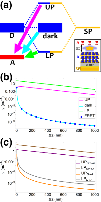
Fig.  1: (a) Schematic energy-level diagram showing the EET transitions from donors strongly coupled to SPs to bare acceptors . The thickness of the horizonal lines denotes the density of states while the thickness of arrows corresponds to rate of transition (thicknesses not drawn to scale). Inset: representation of the EET process from a thick and dense slab of donors (featuring SC to SPs) to a dilute monolayer of acceptors. (b) Rates as a function of donor-acceptor separation $\Delta z$ for EET from donor polariton and dark states to acceptors (lines). The rate from dark states and for the bare-donor FRET (dots), are calculated in the same manner. (c) Contributions of rates for transfer from donor UP and LP to acceptor states due to donor-acceptor and SP-acceptor interactions.

In contrast, strongly coupling the acceptors to a resonant SP mode does not lead to the aforementioned PARET from donors to acceptors (Fig. 2). Making the same assumptions as above about the isotropically oriented and spatially uncorrelated dipoles gives (Section S2.7),

$$\gamma_{\alpha_{A}\leftarrow D} \approx\frac{2\pi}{\hbar N_{D}}\sum_{\vec{k}\in\text{FBZ}}\sum_{i}\left(\sum_{l,m}|c_{A_{\vec{k}}\alpha_{A,\vec{k}}}|^{2}|c_{A_{lm}A_{\vec{k}}}|^{2}|\langle A_{lm}|H_{DA}|D_{i0}\rangle|^{2}\right.$$

$$\left.+|c_{\vec{k}\alpha_{A,\vec{k}}}|^{2}|\langle\vec{k}|H_{DP}|D_{i0}\rangle|^{2}\right)J_{\alpha_{A,\vec{k}},D},$$ (13a)

$$\gamma_{dark_{A}\leftarrow D} =\gamma_{\text{bare FRET}}^{\prime}=\frac{2\pi}{\hbar N_{D}}\sum_{i}\sum_{l,m}|\langle A_{lm}|H_{DA}|D_{i0}\rangle|^{2}J_{A,D}.$$ (13b)

We consider (Fig. 2a) a 50 nm-thick acceptor slab with a concentration of $1\times 10^{9}\text{ \text{molecules}}/\mu\text{m}^{3}$ on top of the 1 nm spacer placed on the metal, and a monolayer of donors with concentration $1\times 10^{4}\text{ }\text{molecules}/\mu\text{m}^{2}$ at varying distances from the acceptors. Notice that $\gamma_{dark_{A}\leftarrow D}$ becomes another bare FRET rate like in Eq. (12b). For $\gamma_{\alpha_{A}\leftarrow D}$, we still see that PRET still dominates over FRET for long distances (Fig. S2). However, due to the suppression of $\gamma_{\alpha_{A}\leftarrow D}$ relative to $\gamma_{dark_{A}\leftarrow D}$ explained in Section 2.1, the limited spatial range of interactions of $H_{DA}$ and $H_{DP}$, and the fact that the donor energy is lower than that of $|\text{UP}_{A,\vec{k}}\rangle$for most $\vec{k}\in\text{FBZ}$ (Fig. S3), the rates to acceptor polaritons fall below fluorescence timescales⁵³ and therefore offer no meaningful enhancements with respect to the bare FRET case (Fig. 2b).

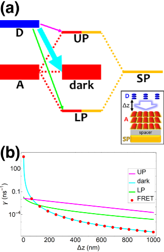
Fig.  2: (a) Schematic energy-level diagram showing the EET transitions from bare donors to acceptors strongly coupled to SPs. The thickness of the horizonal lines denotes the density of states while the thickness of arrows corresponds to rate of transition (thicknesses not drawn to scale). Inset: representation of the EET process from a dilute monolayer of donors to a thick and dense slab of acceptors (featuring SC to SPs). (b) Rates as a function of donor-acceptor separation $\Delta z$ for energy transfer from donors to acceptor polaritons and dark states (lines). The rate to dark states and for bare-acceptor FRET (dots), are calculated in the same manner.

Coupling SPs to acceptors need not, however, be a disapointment. Increasing the collective coupling to $g_{A}=237\text{ meV}$ while keeping $g_{D}=1.7\,\text{meV}$ lifts the acceptor UP energy $\hbar\omega_{UP_{A,\vec{k}}}$ to be higher than $\hbar\omega_{D}$ (Figs. 3a and S4), thus allowing for the carnival effect where the donors and acceptors reverse roles. Due to sufficient spectral overlap between the acceptor UP and donor states (Figs. 3a and S4), transfer from UP occurs at $\sim 100\text{ ns}^{-1}$ for donor-acceptor separation of 1 nm and drops only to $\sim 1\text{ ns}^{-1}$ when this separation approaches $1\text{ }\mu\text{m}$ (Fig. 3b). On the other hand, neither the acceptor dark nor LP states contribute to this reversed PARET given their lack of spectral overlap with the donors and detailed balance (especially at $T=0$), . This result provides the second main conclusion of our work: polaritons offer great versatility to control spectral overlaps without actual chemical modifications to the molecules and can therefore endow them with new physical properties. Before proceeding to simulations for Case $ii$, it should first be noted that while our model neglects intermediate- and far-field donor-acceptor dipole-dipole interactions that become relevant at $\sim\mu\text{m}$ distances, these couplings are expected to be small compared to PRET couplings and therefore should not change our results for Case $i$ qualitatively but can be modeled according to previous literature.⁵⁵ Second, we highlight that the PARET from UP to donors for the donors-only and reversed cases of SC may not be readily observable in experiments due to their competition with fast vibrational relaxation to dark states (~10-100 fs for exciton-microcavity systems),⁵⁶, ⁵⁷, ⁵⁸, ⁵⁹, ⁴² as will be discussed next for both donors and acceptors strongly coupled to SPs.

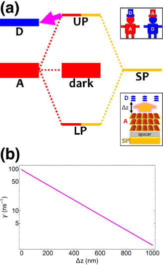
Fig.  3: (a) Schematic energy-level diagram showing the “carnival-effect”-EET role-reversal process from acceptor UP state to bare donors. Insets: (top) cartoon illustrating the “carnival effect” between donors and acceptors and (bottom) representation of the reversed-role EET process from a thick and dense slab of acceptors (featuring SC to SPs) to a dilute monolayer of donors. (b) Rate as a function of donor-acceptor separation $\Delta z$ for energy transfer from acceptor UP to bare donors.

Finally, for strongly coupling both chromophores to the same SP mode, we limit ourselves to donor-acceptor separations $\geq 10$ nm to ignore $H_{DA}$ terms (an approximation validated by the calculations above demonstrating that at such distances, rate contributions of PRET overwhelm those of FRET ). The thickness (35 nm) and density ($1\times 10^{9}\text{ }\text{molecules}/\mu\text{m}^{-3}$) of each slab is large enough to allow for SC of a SP mode to both chromophores separated by $\sim 400$ nm (Fig. S5), even though we set the donor to be in resonance with the SP (Fig. 4). To evaluate the rates derived (Section S3.2) from Eq. (11) under condition $N_{C}\gg N_{xy,C}$ for $C=D,A$, we introduce a spectral density representing intramolecular exciton-phonon coupling of TDBC: $\mathcal{J}_{A}(\omega)\approx\mathcal{J}_{D}(\omega)=\mathcal{J}(\omega)$, where

$$\mathcal{J}(\omega)=\sum_{q\in B_{\text{TDBC}}}\lambda_{q}^{2}\omega_{q}^{2}\frac{\frac{\Gamma/\hbar}{2}}{\pi[(\frac{\Gamma/\hbar}{2})^{2}+(\omega-\omega_{q})^{2}]},$$ (14)

$\Gamma=47\text{ meV}$ is equal to the chromophore decay energy, and $B_{\text{TDBC}}$ is the discrete set (Section S3.2) of localized vibrational modes which significantly couple to each TDBC exciton; such coupling has been experimentally⁵⁶, ⁵⁷, ⁵⁸, ⁵⁹, ⁶⁰ and theoretically supported as the mechanism of vibrational relaxation for the dye⁴², ⁴³, ⁶¹, ⁶², ⁶³; our spectral density has been reconstructed from the works of Agranovich and coworkers ⁴², ⁴³. By placing the donor slab on top of the spacer on the metal and varying the acceptor position on top of the donors (Fig. 4a), we find that for all donor-acceptor separations, the rates of PARET from UP to dark donors ($\sim 10^{5}\text{ ns}^{-1}$) and MP to dark acceptors ($\sim 10^{4}-10^{5}\text{ ns}^{-1}$) are substantially higher compared to those from dark donors to MP ($\sim 10^{3}\text{ ns}^{-1}$) and dark acceptors to LP ($\sim 10^{3}\text{ ns}^{-1}$) (Fig. 4b). These observations are in agreement with our discussion above, where the dark state manifolds act as population sinks due to their high density of states. Indeed, we also notice that the rates for $\text{UP}\rightarrow dark_{D}$ and $\text{MP}\rightarrow dark_{A}$ are enhanced (Fig. 4b) compared to those of $\text{UP}\rightarrow\text{MP}$ and $\text{MP}\rightarrow\text{LP}$, respectively, by approximately $N_{z}=35$, the analytically estimated ratio solely based on the associated density of final states. Another interesting detail seen from Fig. 4b is that the $\text{UP}\rightarrow\text{MP}$ ($\text{MP}\rightarrow\text{LP}$) rate with respect to the interslab distance $\Delta z$ is essentially parallel to that of $\text{UP}\rightarrow dark_{D}$ ($\text{MP}\rightarrow dark_{A}$). This is a consequence of the MP (LP) having mostly donor (acceptor) energy (Fig. S7) and character (Fig. S8) for most points in the FBZ. The $\text{UP}\rightarrow dark_{A}$ and $\text{UP}\rightarrow\text{LP}$ processes behave similarly (Fig S6).

These calculated rates even establish consistency with a number of recent notable experiments. First, our results corroborate the experimental observation of efficient PARET for separated donor and acceptor slabs of cyanine dyes strongly coupled to a microcavity.¹⁷, ¹⁸ While our SP model for the SC of both excitons cannot account for the exact distance-independent PARET¹⁷ amongst donor and acceptor slabs in a microcavity, the rates are essentially constant over hundreds of nanometers due to the slowly decaying SP fields. Additional validation of our theory can be obtained by comparing directly to experimentally fitted rates for a blend of two cyanine dyes where physical separation of the dyes did not significantly change the observed photoluminescence.¹⁸ In our work, we obtained rates that sum across the whole polariton band in the FBZ; in practice, experiments probe polariton photoluminescence around a narrow window of wavevectors close to the anticrossing ($\sim 10^{6}-10^{7}\text{ m}^{-1}$ in ⁴⁸) accounting for a small fraction ($\sim$0.1 %) of the states in the FBZ. If we take this experimental detail into account, we notice good agreements with our theory (see Table 2). As an aside, we note that there are other experimental subtleties, notably competing processes such as cavity leakage (~100-1000 fs for microcavity experiments),⁶⁴, ⁵⁸, ⁵⁹ that we have not considered but may influence the observation of the EET phenomena predicted throughout this work for the two cases of SC.

Given the significant differences between the microcavity-⁶⁵, ⁶⁶ and SP-based⁶⁷ systems, let alone experimental uncertainty, the accordance between our theory and the aforementioned experiments highlights the remarkable robustness of cavity strong-coupling of donor and acceptor excitons as a method for PARET. Moreover, we have arrived at the third main conclusion of this paper: when donor and acceptors are both strongly coupled to a photonic mode, efficient energy exchange over hundreds of nm can occur via vibrational relaxation; more generally, local vibrational couplings can induce nonlocal transitions given sufficient delocalization of the polariton species— irrespective of spatial separation. Seemingly “spooky”, this action at a (far) distance is a manifestation of donor-acceptor entanglement resulting from strong light-matter coupling.⁶⁸ While this relaxation mechanism and entanglement is present in typical molecular aggregates,⁶⁹, ⁷⁰ the novelty in the polariton setup is the remarkable mesoscopic range of interactions that are effectively produced.

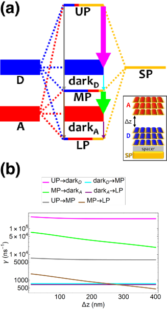
Fig.  4: (a) Schematic energy-level diagram showing the EET transitions among polariton and dark states for both donors and acceptors strongly coupled to SPs. The SP mode is resonant with the donor transition; the donor slab lies 1 nm above the metal and has fixed position ($z>0$) while the acceptor slab is moved in the $+z$-direction to vary $\Delta z$. The thickness of the horizonal lines denotes the density of states while the thickness of arrows corresponds to rate of transition (thicknesses not drawn to scale). Inset: representation of the setup featuring thick and dense slabs for both types of chromophores. (b) Rates for selected downhill transitions as a function of donor-acceptor separation $\Delta z$.

Table 2: Comparison between PARET rates for donor and acceptor cyanine dye J-aggregates strongly coupled to SP (theory) and microcavity (experiment) modes.

$\gamma$	SP (theory)a	SP (theory; experimental polariton bands)b	Microcavity (experiment)c
UP$\rightarrow\text{dark}_{D}$	(10 fs$)^{-1}$	(10 fs$)^{-1}$	(34 fs$)^{-1}$
$\text{dark}_{D}\rightarrow$MP	(1 ps$)^{-1}$	(1000 ps$)^{-1}$	(603 ps$)^{-1}$
MP$\rightarrow\text{dark}_{A}$	(10-100 fs$)^{-1}$ d	(10-100 fs$)^{-1}$ d	(8.5 fs$)^{-1}$
$\text{dark}_{A}\rightarrow$LP	(1 ps$)^{-1}$	(1000 ps$)^{-1}$	(228 ps$)^{-1}$

^aThese orders of magnitudes represent the ranges of rates shown in Fig. 4b. ^bRates accounting for the fact that in typical polariton photoluminescence experiments, only a small fraction ($\sim 0.1$% of wavevectors in the FBZ) of final polariton states near the anticrossing is probed.^{48 c}Photoluminescence-fitted rate constants describing the PARET processes for a blend of J-aggregating NK-2707 (donors) and TDBC (acceptors) cyanine dyes both strongly coupled to a microcavity mode.^{18 d}The corresponding rate (see Fig. 4b) spans two order of magnitudes.

4 Conclusions

In summary, we have theoretically calculated experimentally consistent rates of PARET for various cases of SC. We employed a polariton (plexciton) setup consisting of a metal whose SP modes couple to donor and/or acceptor chromophores. For strongly coupling a single type of chromophore to SPs, we have demonstrated that energy transfer starting from delocalized states can be enhanced due to increased spectral overlap compared to the bare FRET case. Astonshingly, this transfer can remain fast up to 1 $\mu\text{m}$ due to slowly decaying PRET with respect to metal-chromophore separation when compared to the faster decaying interchromophoric dipole-dipole coupling. Also, we have shown that delocalizing the acceptors is a poor strategy to enhance EET starting from the donors, but can lead to an intriguing and efficient role reversal (carnival effect) when starting from the acceptors. These observations shed new light on the timely debate of how to harness coherence to enhance molecular processes.³⁸ Given their generality, they can also be applied to guide the design of polaritonic systems to control other chemical processes that have similar donor-acceptor flavor (e.g., cis-trans isomerization,⁷¹, ³⁰ charge transfer,⁷² dissociation,⁷² electron transfer,³⁷ singlet fission⁷³). Finally, our calculated rates support vibrational relaxation as the mechanism of PARET when both donors and acceptors are strongly coupled to a cavity mode. The results obtained in this work affirm light-matter SC as a promising and novel means to engineer novel interactions between molecular systems across mesoscopic lengthscales, thus opening doors to remote controlled chemistry.

Conflict of interest

There are no conflicts to declare.

Electronic Supplementary Information for “Theory of polariton-assisted remote energy transfer”

^aDepartment of Chemistry and Biochemistry, University of California San Diego, La Jolla, California 92093, United States.

^bDepartment of Chemistry, Department of Physics, and Birck Nanotechnology Center, Purdue University, West Lafayette, IN 47907, United States.

^cQatar Environment and Energy Research Institute, College of Science and Engineering, HBKU, Doha, Qatar.

^dDepartment of Physics, City College, City University of New York, New York 10031, United States.

^eDepartment of Physics, Graduate Center, City University of New York, New York 10016, United States.

^∗To whom correspondence should be addressed. E-mail: jyuenzhou@ucsd.edu

S1 SP modes: additional details

Eq. (3a) and (5) in the main text correspond to Hamiltonians representing the SP modes and their coupling with excitons, respectively. SP modes emerge at the interface of a metal ($z<0$ ) and dielectric medium $(z>0)$ and are assumed to be infinitely delocalized in the $xy$-plane (in practice, they are localized up to a coherence length, but this detail is not important for the time being). For simplicity, the dielectric medium—which contains both donor and acceptor slabs—is taken to have the same real-valued positive dielectric constant $\epsilon_{d}$ at all points within. The metal is assumed to have a Drude permittivity $\epsilon_{m}(\omega)=\epsilon_{\infty}-\frac{\omega_{P}^{2}}{\omega^{2}+i\omega\gamma}$, where $\omega_{P}$ is the plasma frequency, $\epsilon_{\infty}$ is the high-frequency metal permittivity, and $\gamma$ is the damping constant; we set $\gamma\to 0$ in this formalism to get lossless modes and assume that coupling of SPs to environments that induce their relaxation processes is caused by $H_{P}^{(sys-B)}$ (see Eq. (3c)). Here are additional definitions for terms defined in Eqs. (3a) and (5) for each SP mode of in-plane momentum $\vec{k}$ ⁷⁴:

• The SP mode frequency is $\omega_{\vec{k}}=|\vec{k}|c\sqrt{\frac{\epsilon_{d}+\epsilon_{m}(\omega)}{\epsilon_{d}\epsilon_{m}(\omega)}}$, where $c$ is the speed of light in vacuum.

• The evanescent decay constants for the dielectric medium and metal are given by $a_{j\vec{k}}=\sqrt{|\vec{k}|^{2}-\epsilon_{j}(\omega_{\vec{k}})\;(\omega_{\vec{k}}/c)^{2}}$, where $j=d,\,m$.

• The $\vec{k}$-dependent quantization length is $L_{\vec{k}}=\frac{-\epsilon_{m}}{|a_{d\vec{k}}|}+\frac{1}{2|a_{m\vec{k}}|}\left[\frac{d(\omega\epsilon_{m}(\omega))}{d\omega}\Biggr{|}_{\omega=\omega_{\vec{k}}}\left(\frac{\epsilon_{m}-\epsilon_{d}}{\epsilon_{m}}\right)-\epsilon_{m}-\epsilon_{d}\right]$. It was previously reported in the literature ²⁹ with an additional factor of $\frac{1}{2}$; we believe our displayed expression here is correct (see SI in ²²).

The formalism associated with Eq. (5) has been previously utilized in other contexts.^{28, 22, 30, 26}

S2 Case $i$

S2.1 Derivation of EET rate Eq. (7)

Here we derive Eq. (7) of the main text by following works of Sumi⁷⁵ and Cao.³³ This formula describes the rate of transfer from eigenstate $|I\rangle$ to eigenstate $|F\rangle$ of $H_{sys}^{(i)}$ due to perturbation $V^{(i)}$ (Section 2.1), where $|I\rangle$ and $|F\rangle$ are excitonic/polaritonic states for the donor and acceptor, respectively.

For notational simplicity, we define for this derivation $H_{D}^{\prime}$ and $H_{A}^{\prime}$ to be the donor and acceptor Hamiltonian, respectively, such that $H_{C}^{\prime}=H_{C}+H_{P}+H_{CP}$ for the chromophore $C$ that is strongly coupled to a SP mode and $H_{C^{\prime}}^{\prime}=H_{C^{\prime}}$ for the other chromophore $C^{\prime}$, which is weakly coupled to all SP modes. We also introduce the definitions $H_{C}^{\prime(sys/B)}=H_{C}{}^{(sys/B)}+H_{P}^{(sys/B)}$ and $H_{C^{\prime}}^{\prime(sys/B)}=H_{C^{\prime}}^{(sys/B)}$. Then we note for clarity that $H_{A}^{\prime(sys)}|I\rangle=H_{D}^{\prime(sys)}|F\rangle=0$. In addition, $H_{0}^{(i)}=H_{D}^{\prime}+H_{A}^{\prime}$ has eigenstates $\{|\mathcal{D}\rangle\}$ ($\{|\mathcal{A}\rangle\}$) that are also eigenstates of $H_{D}^{\prime}$ ($H_{A}^{\prime}$) and whose excitonic/polaritonic-system component represents only donor (acceptor) but bath component represents all of donor, acceptor, and SPs.

Assuming excitation of donor followed by thermal equilibration occurs before EET, the initial density matrix of the system and bath is assumed to be $\rho_{0}=\rho_{D}^{(sys-B)}\rho_{A}^{(B)}=\sum_{\mathcal{D}}p_{0,\mathcal{D}}|\mathcal{D}\rangle\langle\mathcal{D}|,$ where $p_{0,\mathcal{D}}$ is the equilibrium occupation probability of system-bath state $|\mathcal{D}\rangle$. The constituent density matrices $\rho_{D}^{(sys-B)}=\frac{e^{-H_{D}^{\prime}/k_{B}T}}{\text{tr}e^{-H_{D}^{\prime}/k_{B}T}}$ and $\rho_{A}^{(B)}=\frac{e^{-H_{A}^{\prime(B)}/k_{B}T}}{\text{tr}e^{-H_{A}^{\prime(B)}/k_{B}T}}$ respectively represent the pre-EET equilibrium distribution of donor excited vibronic and acceptor ground vibrational states, in corresponding tensor products with photon states. Then the rate of transfer from $|I\rangle$ to $|F\rangle$ given by Fermi’s golden rule is

$$\gamma_{F\leftarrow I}=\frac{2\pi}{\hbar}\sum_{\mathcal{D},\mathcal{A}}p_{0,\mathcal{D}}|\langle\mathcal{P}_{F}\mathcal{A}|V^{(i)}|\mathcal{P}_{I}\mathcal{D}\rangle|^{2}\delta(\hbar\omega_{\mathcal{A},\mathcal{D}}),$$ (S1)

The state $|\mathcal{P}_{I}\mathcal{D}\rangle$ ($|\mathcal{P}_{F}\mathcal{A}\rangle$) results from projection $\mathcal{P}_{I}=|I\rangle\langle I|$ ($\mathcal{P}_{F}=|F\rangle\langle F|$) of the system component of $|\mathcal{D}\rangle$ ($|\mathcal{A}\rangle$) onto $|I\rangle$ ($|F\rangle$). To express this equation in the (purely electronic/polaritonic) eigenbasis $\{|D\rangle\}\cup\{|A\rangle\}$ of $H_{sys}^{(i)}$, we first use the fact that the bath modes on each type of chromophore are independent (see Eqs. (2b) and (2c)) and write the time-domain expression:

$$\gamma_{F\leftarrow I} =\frac{1}{\hbar^{2}}\int_{-\infty}^{\infty}dt\sum_{\mathcal{D},\mathcal{A}}p_{0,\mathcal{D}}\langle\mathcal{P}_{I}\mathcal{D}|V^{(i)}|\mathcal{P}_{F}\mathcal{A}\rangle\langle\mathcal{P}_{F}\mathcal{A}|e^{-iH_{0}^{(i)}t/\hbar}V^{(i)}e^{iH_{0}^{(i)}t/\hbar}|\mathcal{P}_{I}\mathcal{D}\rangle$$

$$=\frac{1}{\hbar^{2}}\int_{-\infty}^{\infty}dt\sum_{\mathcal{D}}p_{0,\mathcal{D}}\langle\mathcal{P}_{I}\mathcal{D}|V^{(i)}\mathcal{P}_{F}e^{-i(H_{A}^{\prime}+H_{D}^{\prime(B)})t/\hbar}V^{(i)}e^{i(H_{D}^{\prime}+H_{A}^{\prime(B)})t/\hbar}|\mathcal{P}_{I}\mathcal{D}\rangle,$$ (S2)

where in the second line, we have used $\sum_{\mathcal{A}}|\mathcal{P}_{F}\mathcal{A}\rangle\langle\mathcal{P}_{F}\mathcal{A}|e^{-iH_{0}^{(i)}t/\hbar}=\mathcal{P}_{F}e^{-i(H_{A}^{\prime}+H_{D}^{\prime(B)})t/\hbar}$ and $e^{iH_{0}^{(i)}t/\hbar}|\mathcal{P}_{I}\mathcal{D}\rangle=e^{i(H_{D}^{\prime}+H_{A}^{\prime(B)})t/\hbar}|\mathcal{P}_{I}\mathcal{D}\rangle$. Using the independence of the $D,A$ vibrational bath modes, we obtain

$$\gamma_{F\leftarrow I} =\frac{1}{\hbar^{2}}\int_{-\infty}^{\infty}dt\sum_{D^{\prime}}\sum_{A^{\prime}}V_{IF}^{(i)}V_{D^{\prime}A^{\prime}}^{(i)*}\text{tr}_{bD}\{e^{-iH_{D}^{\prime(B)}t/\hbar}\langle D^{\prime}|e^{iH_{D}^{\prime}t/\hbar}\mathcal{P}_{I}\rho_{D}^{(sys-B)}|D\rangle\}\text{tr}_{bA}\{e^{iH_{A}^{\prime(B)}t/\hbar}\rho_{A}^{(B)}\langle F|e^{-iH_{A}^{\prime}t/\hbar}|A^{\prime}\rangle\}$$ (S3)

for $V_{D^{\prime}A^{\prime}}^{(i)}=\langle D^{\prime}|V^{(i)}|A^{\prime}\rangle$; here, $\text{tr}_{bC}$ denotes a trace over the bath degrees of freedom associated with $C$. In the limit of weak exciton-bath coupling, $[e^{iH_{D}^{\prime}t/\hbar},\mathcal{P}_{I}]\approx 0$, and $\langle D^{\prime}|e^{iH_{D}t/\hbar}\rho_{D}^{(sys-B)}|I\rangle\approx 0$ ($\langle F|e^{-iH_{A}t/\hbar}|A^{\prime}\rangle\approx 0$) for $D^{\prime}\neq I$ ($A^{\prime}\neq F$). Then

$$\gamma_{F\leftarrow I}\approx\frac{1}{\hbar^{2}}|V_{FI}^{(i)}|^{2}\int_{-\infty}^{\infty}dt\,\text{tr}_{bD}\{e^{-iH_{D}^{\prime(B)}t/\hbar}\langle I|e^{iH_{D}^{\prime}t/\hbar}\rho_{D}^{(sys-B)}|I\rangle\}\text{tr}_{bA}\{e^{iH_{A}^{\prime(B)}t/\hbar}\rho_{A}^{(B)}\langle F|e^{-iH_{A}^{\prime}t/\hbar}|F\rangle\}.$$ (S4)

To proceed further, let us define the operators

$$\mathcal{I}_{F}(\omega) =\frac{1}{2\pi}\int_{-\infty}^{\infty}dt\,e^{i\omega t}\text{tr}_{bA}\{e^{iH_{A}^{\prime(B)}t/\hbar}\rho_{A}^{(B)}\langle F|e^{-iH_{A}^{\prime}t/\hbar}|F\rangle\},$$ (S5)

$$\mathcal{E}_{I}(\omega) =\frac{1}{2\pi}\int_{-\infty}^{\infty}dt\,e^{-i\omega t}\text{tr}_{bD}\{e^{-iH_{D}^{\prime(B)}t/\hbar}\langle I|e^{iH_{D}^{\prime}t/\hbar}\rho_{D}^{(sys-B)}|I\rangle\},$$ (S6)

representing the spectra for absorption of acceptor state $F$ and emission of donor state $I$, respectively. Also, denote the corresponding spectral overlap as

$$J_{F,I}=\frac{1}{\hbar}\int_{-\infty}^{\infty}d\omega\,\mathcal{E}_{I}(\omega)\mathcal{I}_{F}(\omega).$$ (S7)

Eq. (S4) then yields,

$$\gamma_{F\leftarrow I} \approx\frac{2\pi}{\hbar}|V_{FI}^{(i)}|^{2}J_{F,I},$$ (S8)

which is Eq. (7) of the main text; in other words, the spectral overlap $J_{F,I}$ takes on the role of a density of final states for a Fermi golden rule rate. We note that for our simulations where the donors and acceptors are reversed (see Sections 3 and S2.9), Eq. (S8) still applies except $D,I$ ($A,F$) now refer to acceptors (donors).

S2.2 Estimation of spectral overlaps

As an illustration of the application of our theory, in this subsection, we develop a simplified Lorentzian overlap model to compute $J_{F,I}$ at temperature $T=0$. To write Eqs. (S5) and (S6) as Lorentzian lineshapes, we follow a Feshbach projection operator approach.^{76, 77, 36, 78} While we proceed with the specific case of only donors strongly coupled to a SP (i.e., $H_{A}^{\prime}=H_{A}$ and $H_{D}^{\prime}=H_{D}+H_{P}+H_{DP}$), the derivation can be readily extended to the case of acceptors strongly coupled to a SP.

Define the projectors

$$\mathcal{P}_{A} =\sum_{l,m}|A_{lm}\rangle\langle A_{lm}|\otimes|0_{B}\rangle\langle 0_{B}|,$$ (S9)

$$\mathcal{P}_{D} =\sum_{i,j}|D_{ij}\rangle\langle D_{ij}|\otimes|0_{B}\rangle\langle 0_{B}|+\sum_{\vec{k}\in\text{FBZ}}|\vec{k}\rangle\langle\vec{k}|\otimes|0_{B}\rangle\langle 0_{B}|$$ (S10)

($|0_{B}\rangle$ is the vacuum state for chromophores and SP bath modes, and $|\vec{k}\rangle=a_{\vec{k}}^{\dagger}|0\rangle$), which map vibronic (possibly including photonic component) states onto electronic/photonic—i.e., “bathless”—states. Let the identity on the entire set of degrees of freedom be $1_{sys-B}$ and define the projectors $\mathcal{Q}_{A}=1_{sys-B}-\mathcal{P}_{A}$ and $\mathcal{Q}_{D}=1_{sys-B}-\mathcal{P}_{D}$. Then the time-dependent Schr dinger equation $\frac{d}{dt}|\psi(t)\rangle=-\frac{i}{\hbar}H_{C}^{\prime}|\psi(t)\rangle$ for $C=D,A$ can be rewritten as the coupled equations

$$-\frac{i}{\hbar}\mathcal{P}_{C}H_{C}^{{}^{\prime}}\mathcal{P}_{C}|\mathcal{P}_{C}\psi(t)\rangle-\frac{i}{\hbar}\mathcal{P}_{C}H_{C}^{{}^{\prime}}\mathcal{Q}_{C} |\mathcal{Q}_{C}\psi(t)\rangle=\frac{d}{dt}|\mathcal{P}_{C}\psi(t)\rangle,$$ (S11a)

$$-\frac{i}{\hbar}\mathcal{Q}_{C}H_{C}^{{}^{\prime}}\mathcal{P}_{C}|\mathcal{P}_{C}\psi(t)\rangle-\frac{i}{\hbar}\mathcal{Q}_{C}H_{C}^{{}^{\prime}}Q {}_{C}|\mathcal{Q}_{C}\psi(t)\rangle=\frac{d}{dt}|\mathcal{Q}_{C}\psi(t)\rangle.$$ (S11b)

After the initial condition $|\mathcal{Q}_{C}\psi(0)\rangle=0$, multiplying both sides of Eq. (S11) by $\Theta(t)$, and plugging the formal solution of Eq. (S11b) into Eq. (S11a), we obtain the Green functions $G_{C}(t)=\Theta(t)e^{-iH_{C}^{\prime}t/\hbar}$ which can be Fourier transformed as,³⁶

$$G_{A}(\hbar\omega) =-i\int_{-\infty}^{\infty}dt\,e^{i\omega t}G_{A}(t)=\text{lim}_{\epsilon\to 0^{+}}\frac{1}{\hbar\omega-H_{A}^{(sys)}\otimes|0_{B}\rangle\langle 0_{B}|-R_{A}(\hbar\omega)+i\epsilon},$$ (S12a)

$$G_{D}(\hbar\omega) =-i\int_{-\infty}^{\infty}dt\,e^{i\omega t}G_{D}(t)=\text{lim}_{\epsilon\to 0^{+}}\frac{1}{\hbar\omega-(H_{D}^{(sys)}+H_{P}^{(sys)}+H_{DP})\otimes|0_{B}\rangle\langle 0_{B}|-R_{DP}(\hbar\omega)+i\epsilon},$$ (S12b)

where

$$R_{A}(\hbar\omega) =\mathcal{P}_{A}H_{A}^{(sys-B)}\mathcal{Q}_{A}\frac{1}{\hbar\omega-\mathcal{Q}_{A}H_{A}^{\prime}\mathcal{Q}_{A}+i\epsilon}\mathcal{Q}_{A}H_{A}^{(sys-B)}\mathcal{P}_{A},$$ (S13a)

$$R_{D}(\hbar\omega) =\mathcal{P}_{D}[H_{D}^{(sys-B)}+H_{P}^{(sys-B)}]\mathcal{Q}_{D}\frac{1}{\hbar\omega-\mathcal{Q}_{D}H_{D}^{\prime}\mathcal{Q}_{D}+i\epsilon}\mathcal{Q}_{D}[H_{D}^{(sys-B)}+H_{P}^{(sys-B)}]\mathcal{P}_{D},$$ (S13b)

are the so-called self-energy terms. We next make the partition $R_{C}(\hbar\omega)=\text{Re}R_{C}(\hbar\omega)-\frac{i}{2}\Gamma_{C}(\hbar\omega)$ with $\Gamma_{C}(\hbar\omega)=-2\text{Im}R_{C}(\hbar\omega)$ and assume that the Lamb shifts $\text{Re}R_{C}(\hbar\omega)$ contribute insignificantly when compared to the exciton/SP energies and can thus be neglected. In addition, we take the wide-band approximation that all (diagonal) matrix elements of $\Gamma_{C}(\hbar\omega)$ are constant as a function of $\omega$: $\langle A_{lm},0_{B}|\Gamma_{A}(\hbar\omega)|A_{lm},0_{B}\rangle\approx\Gamma_{A}$, $\langle D_{ij},0_{B}|\Gamma_{D}(\hbar\omega)|D_{ij},0_{B}\rangle\approx\Gamma_{D}$, and $\langle 1_{\vec{k}},0_{B}|\Gamma_{D}(\hbar\omega)|1_{\vec{k}},0_{B}\rangle\approx\Gamma_{P,\vec{k}}$. Then explicitly writing out the respective Hamiltonians in Eq. (S12), we arrive at

$$G_{A}(\hbar\omega) =\text{lim}_{\epsilon\to 0^{+}}\frac{1}{\hbar\omega-(\hbar\omega_{A}-\frac{i}{2}\Gamma_{A})\sum_{l,m}|A_{lm}\rangle\langle A_{lm}|\otimes|0_{B}\rangle\langle 0_{B}|+i\epsilon}$$ (S14a)

$$G_{D}(\hbar\omega) =\text{lim}_{\epsilon\to 0^{+}}\frac{1}{\hbar\omega-[(\hbar\omega_{D}-\frac{i}{2}\Gamma_{D})\sum_{i,j}|D_{ij}\rangle\langle D_{ij}|+\sum_{\vec{k}\in\text{FBZ}}(\hbar\omega_{\vec{k}}-\frac{i}{2}\Gamma_{P,\vec{k}})a_{\vec{k}}^{\dagger}a_{\vec{k}}+H_{DP}]\otimes|0_{B}\rangle\langle 0_{B}|+i\epsilon}$$ (S14b)

$$=\text{lim}_{\epsilon\to 0^{+}}\frac{1}{\hbar\omega-[(\hbar\omega_{D}-\frac{i}{2}\Gamma_{D})\sum_{\vec{k}\in\text{FBZ}}\sum_{d}|d_{\vec{k}}\rangle\langle d_{\vec{k}}|+\sum_{\vec{k}\in\text{FBZ}}\sum_{\alpha}(\hbar\omega_{\alpha_{D,\vec{k}}}-\frac{i}{2}\Gamma_{\alpha_{D,\vec{k}}})|\alpha_{D,\vec{k}}\rangle\langle\alpha_{D,\vec{k}}|]\otimes|0_{B}\rangle\langle 0_{B}|+i\epsilon}.$$ (S14c)

It is intuitively clear that the terms in brackets in the denominators of Eqs. (S14b) and (S14c) correspond to effective Hamiltonians of the donor-SP coupled system. In fact, $\hbar\omega_{\alpha_{D,\vec{k}}}$ and $\Gamma_{\alpha_{D,\vec{k}}}$ are the resulting (real-valued) energy and linewidth of $|\alpha_{D,\vec{k}}\rangle$ (defined just after Eq. (6) in the main text) for $\alpha=\text{UP},\text{LP}$. Comparing those two equations shows that not only can the polariton energies and linewidths be obtained from the diagonalization of a non-Hermitian Hamiltonian for the donors and SP modes, but all dark states have the same energy and linewidth as the bare chromophores.

More precisely, applying the assumption of weak system-bath coupling that was used to derive Eq. (7) and setting $\rho_{C}^{(B)}=|0_{B}\rangle\langle 0_{B}|$ ($T=0$), we can readily relate the expressions for absorption and emission spectra (Eqs. (S5) and (S6), respectively) to matrix elements of the Green’s functions (see Eq. (S12)),

$$\mathcal{I}_{F}(\omega) \approx\frac{1}{2\pi}\text{tr}_{bA}\{e^{iH_{A}^{(B)}t/\hbar}\rho_{A}^{(B)}\langle F|-2\text{Im}G_{A}(\hbar\omega)|F\rangle\}$$

$$=\frac{1}{\pi}\frac{\frac{1}{2}\Gamma_{F}}{(\hbar\omega-\hbar\omega_{I})^{2}+(\frac{1}{2}\Gamma_{F})^{2}},$$ (S15a)

$$\mathcal{E}_{I}(\omega) \approx\frac{1}{2\pi}\text{tr}_{bD}\{e^{-iH_{D}^{(B)}t/\hbar}\rho_{D}^{(B)}\langle I|-2\text{Im}G_{D}(\hbar\omega)|I\rangle\}$$

$$=\frac{1}{\pi}\frac{\frac{1}{2}\Gamma_{I}}{(\hbar\omega-\hbar\omega_{I})^{2}+(\frac{1}{2}\Gamma_{I})^{2}},$$ (S15b)

with $F=A$ ($I=\alpha_{D,\vec{k}},D$) representing any state of type $|A_{lm}\rangle$ ($|\alpha_{\vec{k},D}\rangle,|d_{\vec{k}}\rangle$), and we thus obtain the Lorentzian spectral overlap $J_{F,I}=\frac{1}{\pi}\frac{\frac{\Gamma_{I}+\Gamma_{F}}{2}}{(\frac{\Gamma_{I}+\Gamma_{F}}{2})^{2}+(\hbar\omega_{FI})^{2}}$.

Although we made several approximations to achieve this form, Lorentzian behavior is usually characteristic of lineshapes near their peaks,⁷⁹ leading to overlaps and thus EET rates that are especially relevant when initial and final states are near resonance. In passing, we mention that a different physical mechanism to obtain Lorentzian lineshapes occurs when electronic states are coupled to overdamped Brownian oscillators in the limits of high temperature and fast nuclear dynamics³⁶.

S2.3 Lack of supertransfer enhancement

Here, we demonstrate that even though the donor polariton state is coherently delocalized, the superradiance enhancement of EET to bare acceptors that one could expect^{5, 4} is negligible when taking into account the distance dependence of the involved dipolar interactions. The essence of supertransfer is that a constructive interference of individual donor dipoles in an aggregate can lead to FRET rates that scale as $N$ times a bare FRET rate. However, for this to happen, it is important to have a geometric arrangement where all donors are equidistantly spaced with respect to all acceptors; this is not the case in our problem.

To show this point explicitly, we first evaluate the FRET rate associated with the delocalized donor $|D_{\vec{k}=0}\rangle$ transferring energy to bare acceptors,

$$\gamma_{A\leftarrow D_{\vec{k}=0}}^{FRET} \equiv\frac{2\pi}{\hbar}\sum_{l,m}|\langle A_{lm}|H_{DA}|D_{\vec{k}=\vec{0}}\rangle|^{2}J_{A,D_{\vec{k}=\vec{0}}}$$

$$\approx\frac{2\pi}{\hbar}\mu_{D}^{2}\mu_{A}^{2}\frac{1}{N_{D}}\sum_{l,m}\left|\sum_{i,j}\frac{\kappa_{ijlm}}{r_{ijlm}^{3}}\right|^{2}J_{A,D_{\vec{k}=\vec{0}}},$$ (S16)

where we have approximated $|D_{\vec{k}=0}\rangle$ as a totally symmetric state across all chromophores, $|c_{D_{i^{\prime}j^{\prime}}D_{\vec{k}=0}}|^{2}=\frac{\kappa_{\vec{k}D_{i^{\prime}j^{\prime}}}^{2}}{\sum_{i,j}\kappa_{\vec{k}D_{ij}}^{2}}\approx\frac{1}{N_{D}}$ (see definition of $|C_{\vec{k}}\rangle$ for $C=D,A$ in main text right after Eq. (6)).

Compare Eq. (S16) to the corresponding bare FRET rate

$$\gamma_{\text{bare FRET}}^{\prime\prime}=\frac{2\pi}{\hbar}\mu_{D}^{2}\mu_{A}^{2}\frac{1}{N_{D}}\sum_{l,m}\sum_{i,j}\frac{\kappa_{ijlm}^{2}}{r_{ijlm}^{6}}J_{A,D}.$$ (S17)

Since the separation between donor and acceptor slabs is small compared to their longitudinal ($xy$) dimensions, it is incorrect to approximate the distance $r_{ijlm}$ as constant for all $i,j,l,m$. To see this more precisely,

$$\left|\sum_{i,j}\frac{\kappa_{ijlm}}{r_{ijlm}^{3}}\right|^{2} \leq 4\left(\sum_{i,j}\frac{1}{r_{ijlm}^{3}}\right)^{2}$$

$$=4\left(\rho_{D}\int_{s}^{s+\mathcal{W}}dz\int d\vec{R}\frac{1}{[|\vec{R}-\vec{R}_{l,A}|^{2}+(z-z_{m,A})^{2}]^{\frac{3}{2}}}\right)^{2}$$

$$=4\left(\rho_{D}\int_{s}^{s+\mathcal{W}}dz\int_{0}^{2\pi}d\phi\int_{0}^{\infty}dr\frac{r}{[r^{2}+(z-z_{m,A})^{2}]^{\frac{3}{2}}}\right)^{2}$$

$$\ll\lim_{N_{D}\rightarrow\infty}N_{D}\sum_{i,j}\frac{\kappa_{ijlm}^{2}}{r_{ijlm}^{6}}.$$ (S18)

The finiteness of both the concentration $\rho_{D}$ and the integral over $(r,\phi,z)$ allow going from the third to the fourth line as long as $N_{D}$ is sufficiently large. More precisely, the integral in the third line with respect to $r$ scales as $r^{-1}$ and converges for $z_{m,A}>z_{j,D}$ for all $j$; the sum $\sum_{i,j}\frac{\kappa_{ijlm}^{2}}{r_{ijlm}^{6}}$ in the fourth line can be similarly converted into an integral which converges as $r^{-4}$. We have also used the fact that the squared FRET orientation factor $\kappa_{ijlm}^{2}$ ranges from 0 to 4.⁵⁴ For large enough $N_{D}$, the difference in spectral overlaps $J_{A,D}$ and $J_{A,D_{\vec{k}=\vec{0}}}$ is immaterial. Therefore, if $\gamma_{\text{bare FRET}}^{\prime\prime}\neq 0$, $\gamma_{A\leftarrow D_{\vec{k}=0}}^{FRET}\ll N_{D}\gamma_{\text{bare FRET}}^{\prime\prime}$ and we conclude that the decay of dipolar interactions with respect to distance precludes a supertransfer enhancement^{5, 4} in our problem.

By noticing that $\left|\sum_{i,j}\frac{\kappa_{ijlm}}{r_{ijlm}^{3}}\right|^{2}>\sum_{i,j}\frac{\kappa_{ijlm}^{2}}{r_{ijlm}^{6}}$ (at least when all $\kappa_{ijlm}\geq 0$), and for $J_{A,D}\approx J_{A,D_{\vec{k}=\vec{0}}}$, we still expect a coherence enhancement of EET: $\gamma_{A\leftarrow D_{\vec{k}=0}}^{FRET}>\gamma_{\text{bare FRET}}^{\prime\prime}$. However, this enhancement is quite modest compared to all other effects that we consider in our problem (e.g., PRET contributions).

S2.4 Derivation of rate Eq. (12a) from donor polaritons to acceptors

Here, we derive expressions for EET rates between a multi-layer slab of $N_{D}\gg N_{xy,D}$ donor molecules strongly coupled to a SP and a monolayer of acceptor molecules at $z=z_{0,A}>z_{j,D}$ for all $j$. The polariton states $\alpha=\text{UP},\text{LP}$ are of the form $|\alpha_{D,\vec{k}}\rangle=c_{D_{\vec{k}}\alpha_{D,\vec{k}}}|D_{\vec{k}}\rangle+c_{\vec{k}\alpha_{D,\vec{k}}}|\vec{k}\rangle$, where $|\vec{k}\rangle=a_{\vec{k}}^{\dagger}|0\rangle$ and

$$|D_{\vec{k}}\rangle=\frac{1}{\sqrt{\sum_{i,j}\kappa_{\vec{k}D_{ij}}^{2}e^{-2a_{d\vec{k}}z_{j,D}}}}\sum_{i,j}\kappa_{\vec{k}D_{ij}}e^{-a_{d\vec{k}}z_{j,D}}e^{i\vec{k}\cdot\vec{R}_{i,D}}|D_{ij}\rangle.$$ (S19)

Plugging Eq. (S19) into Eq. (8a), the rate of transfer from donor polariton state $|\alpha_{D,\vec{k}}\rangle$ ($\alpha=\text{UP},\text{LP}$) to acceptors is

$$\gamma_{A\leftarrow\alpha_{D,\vec{k}}} =\frac{2\pi}{\hbar}\sum_{l}\left|\langle A_{l0}|H_{DA}+H_{AP}|\alpha_{D}\rangle\right|^{2}J_{A\alpha_{D,\vec{k}}}$$

$$=\frac{2\pi}{\hbar}\sum_{l}\left|\langle A_{l0}|H_{DA}+H_{AP}|\left(c_{D_{\vec{k}}\alpha_{D,\vec{k}}}\sum_{i,j}\frac{\kappa_{\vec{k}D_{ij}}e^{-a_{d\vec{k}}z_{j,D}}e^{i\vec{k}\cdot\vec{R}_{i,D}}}{\sqrt{\sum_{i,j}\kappa_{\vec{k}D_{ij}}^{2}e^{-2a_{d\vec{k}}z_{j,D}}}}|D_{ij}\rangle+c_{\vec{k}\alpha_{D,\vec{k}}}|\vec{k}\rangle\right)\right|^{2}J_{A,\alpha_{D,\vec{k}}}.$$ (S20)

For simplicity, we next assume the chromophore TDMs are isotropically distributed and orientationally uncorrelated,

$$\gamma_{A\leftarrow\alpha_{D,\vec{k}}} =|c_{D_{\vec{k}}\alpha_{D,\vec{k}}}|^{2}\frac{2\pi}{\hbar}N_{A}\sum_{i,j}\Bigg{(}\frac{e^{-2a_{d\vec{k}}z_{j}}}{N_{xy,D}\sum_{j}e^{-2a_{d\vec{k}}z_{j,D}}}\Bigg{)}\frac{\mu_{D}^{2}\mu_{A}^{2}\langle\kappa_{FRET}^{2}\rangle}{r_{ij}^{6}}J_{A\alpha_{D,\vec{k}}}$$

$$\qquad+|c_{\vec{k}\alpha_{D,\vec{k}}}|^{2}\frac{2\pi}{\hbar}\rho_{A}^{(2D)}\mu_{A}^{2}\langle\kappa_{LM,\vec{k}}^{2}\rangle\frac{\hbar\omega_{\vec{k}}}{2\epsilon_{0}L_{\vec{k}}}e^{-2a_{d\vec{k}}z_{0,A}}J_{A\alpha_{D,\vec{k}}},$$ (S21a)

where $r_{ij}$ is distance between acceptor at $(0,0,z_{0,A})$ and donor $ij$, $\rho_{A}^{(2D)}=\frac{N_{xy,A}}{S}$ is the concentration of acceptors per unit area, the isotropically averaged orientation factors for FRET and light-matter interaction are $\langle\kappa_{FRET}^{2}\rangle=\langle\kappa_{ijl0}^{2}\rangle=\frac{2}{3}$⁵⁴, and $\langle\kappa_{LM,\vec{k}}^{2}\rangle=\langle\kappa_{\vec{k}D_{ij}}^{2}\rangle=\frac{2}{3}+\frac{1}{3}\frac{|\vec{k}|^{2}}{a_{d\vec{k}}^{2}}$²⁸. Eq. (S21a) shows that the isotropic distribution of dipoles and the lack of correlations amongst their orientations yields an incoherently averaged rate over the populations of exciton (first term) and SP (second term). Furthermore, Eq. (13b) of the main text is a less explicit form of Eq. (S21a) that follows from using the approximation $\frac{e^{-2a_{d\vec{k}}z_{j,D}}}{N_{xy,D}\sum_{j}e^{-2a_{d\vec{k}}z_{j,D}}}\approx|c_{D_{ij}D_{\vec{k}}}|^{2}=\frac{\kappa_{\vec{k}D_{ij}}^{2}e^{-2a_{d\vec{k}}z_{j,D}}}{\sum_{i,j}\kappa_{\vec{k}D_{ij}}^{2}e^{-2a_{d\vec{k}}z_{j,D}}}$ (i.e., ignoring the orientational dependence of the exciton populations).

In obtaining Eq. (S21a), we have utilized the following approximations which are valid for large $N_{D}$:

$$\left\langle\frac{\kappa_{\vec{k}D_{ij}}\kappa_{ijl0}\kappa_{\vec{k}D_{i^{\prime}j^{\prime}}}\kappa_{i^{\prime}j^{\prime}l0}}{\sum_{i,j}\kappa_{\vec{k}D_{ij}}^{2}e^{-2a_{d\vec{k}}z_{j,D}}}\right\rangle \approx\frac{\langle\kappa_{\vec{k}D_{ij}}\kappa_{ijl0}\kappa_{\vec{k}D_{i^{\prime}j^{\prime}}}\kappa_{i^{\prime}j^{\prime}l0}\rangle}{\sum_{i,j}\langle\kappa_{\vec{k}D_{ij}}^{2}\rangle e^{-2a_{d\vec{k}}z_{j,D}}}=\frac{\langle\kappa_{\vec{k}D_{ij}}\kappa_{ijl0}\kappa_{\vec{k}D_{i^{\prime}j^{\prime}}}\kappa_{i^{\prime}j^{\prime}l0}\rangle}{\langle\kappa_{LM}^{2}\rangle N_{xy,D}\sum_{j}e^{-2a_{d\vec{k}}z_{j,D}}},$$ (S22a)

$$\left\langle\frac{\kappa_{\vec{k}D_{ij}}\kappa_{ijlm}\kappa_{\vec{k}A_{l0}}}{\sqrt{\sum_{i,j}\kappa_{\vec{k}D_{ij}}^{2}e^{-2a_{d\vec{k}}z_{j,D}}}}\right\rangle \approx\frac{\langle\kappa_{\vec{k}D_{ij}}\kappa_{ijlm}\kappa_{\vec{k}A_{l0}}\rangle}{\langle\sqrt{\sum_{i,j}\kappa_{\vec{k}D_{ij}}^{2}e^{-2a_{d\vec{k}}z_{j,D}}}\rangle}.$$ (S22b)

In addition, we have applied a mean-field approach to the orientational factors,

$$\langle\kappa_{\vec{k}D_{ij}}\kappa_{ijl0}\kappa_{\vec{k}D_{{}^{\prime}i^{\prime}j}}\kappa_{i^{\prime}j^{\prime}l0}\rangle \approx\langle\kappa_{\vec{k}D_{ij}}\kappa_{\vec{k}D_{{}^{\prime}i^{\prime}j}}\rangle\langle\kappa_{ijl0}\kappa_{i^{\prime}j^{\prime}l0}\rangle=\langle\kappa_{LM,\vec{k}}^{2}\rangle\langle\kappa_{FRET}^{2}\rangle\delta_{(i,j),(i^{\prime}j^{\prime})},$$ (S23a)

$$\langle\kappa_{\vec{k}D_{ij}}\kappa_{ijl0}\kappa_{\vec{k}A_{l0}}\rangle \approx\langle\kappa_{\vec{k}D_{ij}}\kappa_{\vec{k}A_{l0}}\rangle\langle\kappa_{ijl0}\rangle=0.$$ (S23b)

In the continuum limit, Eq. (S21a) reads,

$$\gamma_{A\leftarrow\alpha_{D,\vec{k}}}=\frac{2\pi}{\hbar}\rho_{A}^{(2D)}\left[|c_{D_{\vec{k}}a_{D,\vec{k}}}|^{2}\mu_{D}^{2}\mu_{A}^{2}\langle\kappa_{FRET}^{2}\rangle\frac{\int_{s}^{s+\mathcal{W}}dze^{-2a_{d\vec{k}}z}\frac{\pi}{2(z_{0,A}-z)^{4}}}{\frac{e^{-2a_{d\vec{k}}(s+\mathcal{W})}-e^{-2a_{d\vec{k}}s}}{-2a_{d\vec{k}}}}+|c_{\vec{k}\alpha_{D,\vec{k}}}|^{2}\mu_{A}^{2}\langle\kappa_{LM,\vec{k}}^{2}\rangle\frac{\hbar\omega_{\vec{k}}}{2\epsilon_{0}L_{\vec{k}}}e^{-2a_{d\vec{k}}z_{0,A}}\right]J_{A\alpha_{D,\vec{k}}},$$ (S24)

where the base of the donor slab is located at $z=s$ and its thickness is $\mathcal{W}$ (while the integral over $z$ is analytical, it is complicated and does not shed much insight into the problem).

S2.5 Derivation of rate Eq. (12b) from donor dark states to acceptors

Here, we show that the rate (Eq. (8b)) of EET from donor dark states to a spatially separated monolayer of bare acceptors at $z=z_{0,A}$ converges to the bare FRET rate $\gamma_{\text{bare FRET}}$ in Eq. (12b) assuming that $N_{D}\gg N_{xy,D}$ and all donor and acceptor TDMs are isotropically oriented and uncorrelated. The steps applied in this subsection can be extended in a straightforward manner to establish this result for multiple layers in the acceptor slab. This result is intuitively expected given that the dark states are purely excitonic and centered at the original transition frequency $\omega_{D}$; furthermore, the density of dark states is close to the original density of bare donor states. Our derivation here relies on Lorentzian lineshapes for the dark donor and acceptor states (see Section S2.2); however, we anticipate the conclusions to hold for more general lineshapes under certain limits.

Section S2.2 specifically reveals that weak system-bath coupling and $T=0$ allow the lineshape of each dark state $|d_{D,\vec{k}}\rangle$ to be expressed as a Lorentzian with peak energy and linewidth identical to that of bare donors, leading to $J_{A,d_{D,\vec{k}}}=J_{A,D}$. Connecting this finding to the relevant rate expression, we can rewrite Eq. (8b) of the main text for an acceptor monolayer as

$$\gamma_{A\leftarrow dark_{D}} =\frac{2\pi}{\hbar}\frac{1}{N_{D}-N_{xy,D}}\sum_{l}\left[\sum_{i,j}|\langle A_{l0}|H_{DA}|D_{ij}\rangle|^{2}-\sum_{\vec{k}\in\text{FBZ}}|\langle A_{l0}|H_{DA}|D_{\vec{k}}\rangle|^{2}\right]J_{A,D}.$$ (S25)

We have used the relation $\sum_{\vec{k}\in\text{FBZ}}\sum_{d}|d_{\vec{k}}\rangle\langle d_{\vec{k}}|=1_{D}^{(sys)}-\sum_{\vec{k}\in\text{FBZ}}|D_{\vec{k}}\rangle\langle D_{\vec{k}}|$ for donor (electronic) identity $1_{D}^{(sys)}$. Assuming $N_{z,D}\gg 1$ (equivalent to $N_{D}\gg N_{xy,D}$ ), we have

$$\gamma_{A\leftarrow dark_{D}} =\frac{2\pi}{\hbar}\frac{1}{N_{D}}\sum_{l}\sum_{i,j}|\langle A_{l}|H_{DA}|D_{ij}\rangle|^{2}J_{A,D}-\frac{2\pi}{\hbar}\frac{1}{N_{D}}\sum_{l}\sum_{\vec{k}\in\text{FBZ}}|\langle A_{l}|H_{DA}|D_{\vec{k}}\rangle|^{2}J_{A,D}.$$ (S26)

We note that the first term is exactly $\gamma_{\text{bare FRET}}^{\prime}$. Applying the arguments from the derivation (Section S2.4, including the orientational averaging approximations of Eqs. (S22) and (S23)) of the rate of EET from donor polaritons to acceptors, as well as the continuum approximation, we obtain

$$\gamma_{A\leftarrow dark_{D}} =\frac{2\pi}{\hbar}\rho_{A}^{(2D)}\mu_{D}^{2}\mu_{A}^{2}\langle\kappa_{FRET}^{2}\rangle\left[\frac{\int_{s}^{s+\mathcal{W}}dz\frac{\pi}{2(z_{0,A}-z)^{4}}}{\mathcal{W}}-\frac{1}{N_{D}}\sum_{\vec{k}\in\text{FBZ}}\frac{\int_{s}^{s+\mathcal{W}}dze^{-2a_{d\vec{k}}z}\frac{\pi}{2(z_{0,A}-z)^{4}}}{\int_{s}^{s+\mathcal{W}}dze^{-2a_{d\vec{k}}z}}\right]J_{AD}.$$ (S27)

Next, we make the approximation $\frac{\int_{s}^{s+\mathcal{W}}dze^{-2a_{d\vec{k}}z}\frac{\pi}{2(z_{0,A}-z)^{4}}}{\int_{s}^{s+\mathcal{W}}dze^{-2a_{d\vec{k}}z}}\approx\frac{\int_{s}^{s+\mathcal{W}}dz\frac{\pi}{2(z_{0,A}-z)^{4}}}{\mathcal{W}}$, where the lefthand side is a weighted average of $\frac{\pi}{2(z_{0,A}-z)^{4}}$. Then we can write

$$\gamma_{A\leftarrow dark_{D}}\approx\frac{2\pi}{\hbar}\rho_{A}^{(2D)}\mu_{D}^{2}\mu_{A}^{2}\langle\kappa_{FRET}^{2}\rangle\left(1-\frac{1}{N_{z,D}}\right)\frac{\int_{s}^{s+\mathcal{W}}dz\frac{\pi}{2(z_{0,A}-z)^{4}}}{\mathcal{W}}J_{AD},$$ (S28)

where we have used $\sum_{\vec{k}\in\text{FBZ}}=N_{xy,D}$ in obtaining this equation. With $N_{z,D}\gg 1$, we arrive at

$$\gamma_{A\leftarrow dark_{D}} \approx\frac{2\pi}{\hbar}\rho_{A}^{(2D)}\mu_{D}^{2}\mu_{A}^{2}\langle\kappa_{FRET}^{2}\rangle\frac{\frac{\pi}{6}\left[\frac{1}{(z_{0,A}-s-\mathcal{W})^{3}}-\frac{1}{(z_{0,A}-s)^{3}}\right]}{\mathcal{W}}J_{AD}.$$ (S29)

This expression is exactly the bare FRET rate $\gamma_{\text{bare FRET}}$ of Eq. (13b) under the aforementioned assumptions of infinitely extended slab along the $xy$ plane, translational symmetry, orientational averaging, and the continuum limit.

S2.6 Additional simulation notes/data for strongly coupling donor

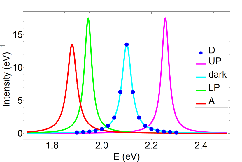
Fig.  S1: SC of SPs to donors. Lorentzian spectra for the donor polariton and dark states, as well as the bare donors and acceptors.

S2.7 Derivation of simulated rates for strongly coupling acceptors

The simulated rates for EET from a monolayer of bare donor at $z=z_{0,D}>z_{m,A}$ for all $m$ to acceptor polariton/dark states asssuming a thick acceptor slab ($N_{A}\gg N_{xy,A}$), orientational averaging and no correlations for the TDMs $\vec{\mu}_{A_{lm}}$ are given by

$$\gamma_{\alpha_{A}\leftarrow D} =\frac{1}{\hbar}\int_{0}^{\pi/a}dk\,k\left[|c_{A_{\vec{k}}\alpha_{A,\vec{k}}}|^{2}\mu_{D}^{2}\mu_{A}^{2}\langle\kappa_{FRET}^{2}\rangle\frac{\int_{s}^{s+\mathcal{W}}dze^{-2a_{d\vec{k}}z}\frac{\pi}{2(z_{0,D}-z)^{4}}}{\frac{e^{-2a_{d\vec{k}}(s+\mathcal{W})}-e^{-2a_{d\vec{k}}s}}{-2\alpha_{d\vec{k}}}}+|c_{\vec{k}\alpha_{A,\vec{k}}}|^{2}\mu_{D}^{2}\langle\kappa_{LM}^{2}\rangle\frac{\hbar\omega_{\vec{k}}}{2\epsilon_{0}L_{\vec{k}}}e^{-2a_{d\vec{k}}z_{0,D}}\right]J_{\alpha_{A,\vec{k}}D}$$ (S30a)

$$\gamma_{dark_{A}\leftarrow D} =\frac{2\pi}{\hbar}\rho_{A}\mu_{D}^{2}\mu_{A}^{2}\langle\kappa_{FRET}^{2}\rangle\frac{\pi}{6}\left[\frac{1}{(z_{0,D}-s-\mathcal{W})^{3}}-\frac{1}{(z_{0,D}-s)^{3}}\right]J_{AD}=\gamma_{\text{bare FRET}}^{\prime}.$$ (S30b)

Here, the thickness of the acceptor slab is $\mathcal{W}$, its base is located at $z=s$, and its (three-dimensional) concentration is $\rho_{A}=\frac{N_{A}}{S\mathcal{W}}$. The derivation of Eq. (S30) starts with the preliminary rate expression in Eq. (9) of the main text and proceeds analogously to those in Sections S2.4 and S2.5, respectively. In contrast to Eq. (S24), Eq. (S30a) also sums over the final polariton $\vec{k}$ modes, yielding a integral rate upon invoking the continuum-limit transformation $\sum_{\vec{k}\in\text{FBZ}}\rightarrow\frac{S}{(2\pi)^{2}}\int_{0}^{2\pi}d\phi\int_{0}^{\pi/a}dk\,k$ for acceptor lattice spacing $a$. Eq. (S30) is a more explicit form of Eqs. 13 in the main text.

We now consider the case when

$$\frac{1}{N_{xy,A}}\sum_{\vec{k}\in\text{FBZ}}|\langle\vec{k}|H_{DP}|D_{i0}\rangle|^{2}<\frac{1}{N_{A}}\sum_{l,m}|\langle A_{lm}|H_{DA}|D_{i0}\rangle|^{2},$$ (S31)

in other words, the average PRET coupling intensity is smaller than that of FRET; this happens when the donor-acceptor separation lies within the typical FRET range (1-10 nm). As we next show, the EET rate from a monolayer of bare donors to acceptor polariton band $\alpha_{A}$ is consequently much smaller than the bare FRET rate ($\gamma_{\text{bare FRET}}^{\prime\prime}$ in Eq. (S17)) as $N_{A}\gg N_{xy,A}$ (i.e., $N_{z,A}\gg 1$), for isotropic and uncorrelated orientational distribution of TDMs $\vec{\mu}_{A_{ij}}$. The steps taken here resemble those employed in Section S2.5. Starting from Eq. (13a), we utilize $|c_{A_{lm}A_{\vec{k}}}|^{2}\approx\frac{1}{N_{A}}$ to obtain

$$\gamma_{\alpha_{A}\leftarrow D} \approx\frac{2\pi}{\hbar N_{D}}\sum_{\vec{k}\in\text{FBZ}}\sum_{i}\left[|c_{A_{\vec{k}}\alpha_{A,\vec{k}}}|^{2}\sum_{l,m}\frac{1}{N_{A}}|\langle A_{lm}|H_{DA}|D_{i0}\rangle|^{2}+|c_{\vec{k}\alpha_{A,\vec{k}}}|^{2}|\langle\vec{k}|H_{DP}|D_{i0}\rangle|^{2}\right]J_{\alpha_{A,\vec{k}},D}$$

$$\leq\frac{2\pi}{\hbar N_{D}}\sum_{i}\sum_{l,m}|\langle A_{lm}|H_{DA}|D_{i0}\rangle|^{2}\frac{1}{N_{z,A}}\max_{\vec{k}\in\text{FBZ}}J_{\alpha_{A,\vec{k}},D}$$

$$\qquad+\frac{2\pi}{\hbar N_{D}}\sum_{i}\sum_{\vec{k}\in\text{FBZ}}|\langle\vec{k}|H_{DP}|D_{i0}\rangle|^{2}\max_{\vec{k}\in\text{FBZ}}J_{\alpha_{A,\vec{k}},D}$$

$$\ll\frac{2\pi}{\hbar N_{D}}\sum_{i}\sum_{l,m}|\langle A_{lm}|H_{DA}|D_{i0}\rangle|^{2}J_{A,D}$$

$$=\gamma_{\text{bare FRET}}^{\prime\prime},$$ (S32)

where the second inequality holds for sufficiently large $N_{z,A}$ such that $\frac{2}{N_{z,A}}\max_{\vec{k}\in\text{FBZ}}J_{\alpha_{A,\vec{k}},D}\ll J_{A,D}$. This result can be physically interpreted as follows: $\gamma_{\text{bare FRET}}^{\prime\prime}$ and $\gamma_{\alpha_{A}\leftarrow D}^{FRET}$ scale as the number of final states $N_{A}$ and $N_{xy,A}\ll N_{A}$, respectively.

S2.8 Additional simulation notes/data for strongly coupling acceptors

We note that the rates from donors to polariton bands (Eq. S30a) were calculated numerically. In particular, the integrals over $k$ were calculated via the trapezoid rule using 2000 intervals.

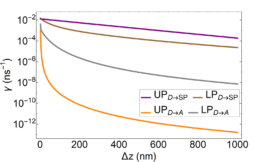
Fig.  S2: SC of SPs to acceptors. Contributions of EET rates from donors to acceptor UP and LP due to donor-acceptor and SP-donor interactions.

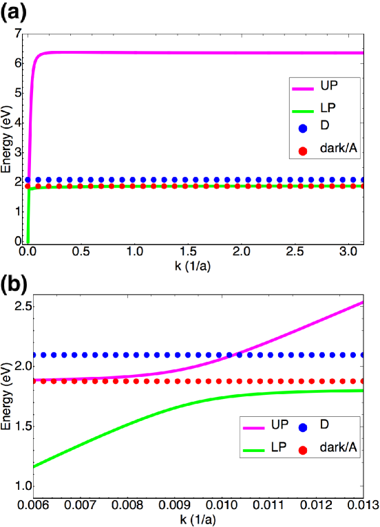
Fig.  S3: SC of SPs to acceptors. (a) Dispersion curve in the FBZ. The value $a=1\times 10^{-9}\text{ m}$ is the inter-chromophoric lattice spacing for the acceptor slab. (b) Expanded view of dispersion curve at region of anticrossing characteristic of SC.

S2.9 Simulations for the “carnival effect”

For this simulation, the coupling is strong enough such that the UP is higher in energy than the bare donors. Thus, the acceptor UP becomes a donor and the donors turn into acceptors. Thus, we use the rate Eq. (S24) derived for the case of strongly-coupling SP to donors only for transfer from a polariton state with the labels $D$ and $A$ interchanged.

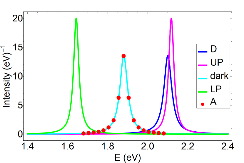
Fig.  S4: Carnival effect or EET role-reversal. Lorentzian spectra for the acceptor polariton and dark states, as well as the bare donors and acceptors.

S3 Case $ii$

S3.1 Derivation: EET rates Eqs. (11)

In this section, we show how to derive the EET rates in Eqs. (11) of the main text between polariton/dark states when both donors and acceptors are strongly coupled to an SP mode. While we only derive rate Eq. (11a) in significant detail, Eqs. (11b) and (11c) can be analogously obtained in essentially the same manner.

Excitons coupled to the $\vec{k}$-th SP mode produce polariton states of the form $|\alpha_{\vec{k}}\rangle=c_{D_{\vec{k}}\alpha_{\vec{k}}}|D_{\vec{k}}\rangle+c_{A_{\vec{k}}\alpha_{\vec{k}}}|A_{\vec{k}}\rangle+c_{\vec{k}\alpha_{\vec{k}}}|\vec{k}\rangle$. As discussed in the main text, the perturbation $V^{(ii)}$ due to the chromophore and photon baths induces transitions between the UP, MP, LP and dark states of donors and acceptors,

$$V^{(ii)} =\sum_{C}\sum_{i,j}|C_{ij}\rangle\langle C_{ij}|\sum_{q}\lambda_{q,C}\hbar\omega_{q,C}(b_{q,C_{ij}}^{\dagger}+\text{h.c.})+\sum_{\vec{k}}\sum_{q}g_{q,\vec{k}}(b_{q,P}^{\dagger}a_{\vec{k}}+\text{h.c.}),$$ (S33)

where $C=D,A$. Given the locality of vibronic coupling, the first term only couples two states that share the same chromophores. On the other hand, the second term does not couple different polariton/dark states because it represents radiative and Ohmic losses from the SP modes. The EET rate from a single polariton state $|\alpha_{\vec{k}}\rangle$ to the polariton band $\beta$ can then be calculated by invoking Fermi’s Golden Rule,

$$\gamma_{\beta\leftarrow\alpha_{\vec{k}}} =\sum_{\vec{k}^{\prime}\in\text{FBZ}}\sum_{C}|c_{C_{\vec{k}^{\prime}}\beta_{\vec{k}^{\prime}}}|^{2}|c_{C_{\vec{k}}\alpha_{\vec{k}}}|^{2}\sum_{i,j}|c_{C_{ij}C_{\vec{k}^{\prime}}}|^{2}|c_{C_{ij}C_{\vec{k}}}|^{2}$$

$$\qquad\times\frac{2\pi}{\hbar^{2}}\sum_{L^{\prime}}\sum_{L}p_{L_{C_{ij}}}|\langle L^{\prime}_{C_{ij}}|\sum_{q}\lambda_{q,C}\hbar\omega_{q,C}(b_{q,C_{ij}}^{\dagger}+b_{q,C_{ij}})|L{}_{C_{ij}}\rangle|^{2}\delta(\omega_{\beta_{\vec{k}^{\prime}}\alpha_{\vec{k}}}+\omega_{L^{\prime}_{C_{ij}}L{}_{C_{ij}}}).$$ (S34)

$|L_{C_{ij}}\rangle$ refers to a local bath state of molecule $C_{ij}$ and $p_{L_{C_{ij}}}$ is the thermal probability to populate it. Assuming that all molecules of the same type $C$ (donor or acceptor) feature the same bath modes, we can associate the single-molecule rate

$$\frac{2\pi}{\hbar^{2}}\sum_{L^{\prime}}\sum_{L}p_{L_{C_{ij}}}|\langle L^{\prime}_{C_{ij}}|\sum_{q}\lambda_{q,C}\hbar\omega_{q,C}(b_{p,C_{ij}}^{\dagger}+b_{p,C_{ij}})|L_{C_{ij}}\rangle|^{2}\delta(\omega+\omega_{L^{\prime}_{C_{ij}}L_{C_{ij}}}) =\mathcal{R}_{C}(\omega)$$ (S35)

which can be readily related to a spectral density, as explained in the main text. Then we arrive at the compact expression,

$$\gamma_{\beta\leftarrow\alpha_{\vec{k}}}=\sum_{\vec{k}^{\prime}\in\text{FBZ}}\sum_{C}|c_{C_{\vec{k}^{\prime}}\beta_{\vec{k}^{\prime}}}|^{2}|c_{C_{\vec{k}}\alpha_{\vec{k}}}|^{2}\sum_{i,j}|c_{C_{ij}C_{\vec{k}^{\prime}}}|^{2}|c_{C_{ij}C_{\vec{k}}}|^{2}\mathcal{R}_{C}(\omega_{\beta_{\vec{k}^{\prime}}\alpha_{\vec{k}}}),$$ (S36)

which is exactly Eq. (11a) of the main text.

To derive the average rate Eq. (11b) from dark states of chromophore $C$ to the polariton band $\alpha$, we begin with

$$\gamma_{\alpha\leftarrow dark_{C}}=\frac{2\pi}{\hbar^{2}}\sum_{\vec{k}^{\prime}\in\text{FBZ}}\frac{1}{N_{C}-N_{xy,C}}\sum_{\vec{k}\in\text{FBZ}}\sum_{d}\sum_{i^{\prime}j^{\prime}}\sum_{L^{\prime}}\sum_{i^{\prime\prime}j^{\prime\prime}}\sum_{L}p_{L_{C_{i^{\prime\prime}j^{\prime\prime}}}}|\langle\alpha_{\vec{k}^{\prime}},L^{\prime}_{C_{i^{\prime}j^{\prime}}}|V^{(ii)}|d_{C,\vec{k}},L{}_{C_{i^{\prime\prime}j^{\prime\prime}}}\rangle|^{2}\delta(\omega_{\alpha_{\vec{k}^{\prime}}C}+\omega_{L^{\prime}_{C_{i^{\prime}j^{\prime}}}L{}_{C_{i^{\prime\prime}j^{\prime\prime}}}}).$$ (S37)

Similarly, the derivation of rate Eq. (11c) from polariton state $|\alpha_{\vec{k}}\rangle$ to the same dark states starts at

$$\gamma_{dark_{C}\leftarrow\alpha_{\vec{k}}}=\frac{2\pi}{\hbar^{2}}\sum_{\vec{k}\in\text{FBZ}}\sum_{d}\sum_{i^{\prime}j^{\prime}}\sum_{L^{\prime}}\sum_{i^{\prime\prime}j^{\prime\prime}}\sum_{L}p_{L_{C_{i^{\prime\prime}j^{\prime\prime}}}}|\langle d_{C,\vec{k}^{\prime}},L^{\prime}_{C_{i^{\prime}j^{\prime}}}|V^{(ii)}|\alpha_{\vec{k}},L{}_{C_{i^{\prime\prime}j^{\prime\prime}}}\rangle|^{2}\delta(\omega_{C\alpha_{\vec{k}}}+\omega_{L^{\prime}_{C_{i^{\prime}j^{\prime}}}L{}_{C_{i^{\prime\prime}j^{\prime\prime}}}}).$$ (S38)

We note that the presence of the prefactor $\frac{1}{N_{C}-N_{xy,C}}$ in Eq. (S37) and lack thereof in Eq. (S38) is due to the asymmetry of Fermi’s Golden Rule: in the former equation, dark states serve as the initial state and thus the term for each state is weighted by its occupation probability, which we have assumed to be uniform at $\frac{1}{N_{C}-N_{xy,C}}$ given their degeneracy.

S3.2 Simulated rates

In this section, we present the rates used in our simulations for both donors and acceptors strongly coupled to a SP assuming (as discussed in the main text) orientationally averaged TDMs $\vec{\mu}_{C_{ij}}$, $N_{xy,D}=N_{xy,A}=N_{xy}$, and $N_{z,C}\gg 1$ for $C=D,A$.

The overlap between $|C_{ij}\rangle$ and the collective mode $|C_{\vec{k}}\rangle$ can be written as $|c_{C_{ij}C_{\vec{k}}}|=\frac{\kappa_{\vec{k}C_{ij}}e^{-a_{d\vec{k}}z_{j,C}}}{\sqrt{\sum_{i,j}\kappa_{\vec{k}C_{ij}}^{2}e^{-2a_{d\vec{k}}z_{j,C}}}}$ and plugged into Eq. (11a) to obtain the rate for EET from polariton state $|\alpha_{\vec{k}}\rangle$ to band $\beta$:

$$\gamma_{\beta\leftarrow\alpha_{\vec{k}}}=\frac{1}{2\pi}\sum_{C}\frac{|c_{C_{\vec{k}}\alpha}|^{2}}{\rho_{C}\frac{e^{-2a_{d\vec{k}}(s_{C}+\mathcal{W}_{C})}-e^{-2a_{d\vec{k}}s_{C}}}{-2a_{d\vec{k}}}}\int_{0}^{\pi/a}dk^{\prime}\,k^{\prime}|c_{C_{\vec{k}}\beta}|^{2}\frac{\frac{e^{-2(a_{d\vec{k}}+a_{d\vec{k}^{\prime}})(s_{D}+\mathcal{W}_{D})}-e^{-2(a_{d\vec{k}}+a_{d\vec{k}^{\prime}})s_{D}}}{-4a_{d\vec{k}^{\prime}}}}{\frac{e^{-2a_{d\vec{k}^{\prime}}(s_{D}+\mathcal{W}_{D})}-e^{-2a_{d\vec{k}^{\prime}}s_{D}}}{-2a_{d\vec{k}^{\prime}}}}\mathcal{R}_{D}(\omega_{\beta_{\vec{k}^{\prime}}\alpha_{\vec{k}}}),$$ (S39)

where we have applied orientational averaging of the TDMs under the approximation $\langle|c_{C_{ij}C_{\vec{k}}}|^{2}\rangle\approx\frac{e^{-2a_{d\vec{k}}z_{j,C}}}{N_{xy}\sum_{j}e^{-2a_{d\vec{k}}z_{j,C}}}$ (Section S2.4) and the $\vec{k}$-space continuum-limit transformation (Section S2.7).

The derivation of the EET rate from polariton $|\alpha_{\vec{k}}\rangle$ to dark states is quite alike that of Section S2.5. We can write Eq. (11c) as

$$\gamma_{dark_{C}\leftarrow\alpha_{\vec{k}}} =|c_{C_{\vec{k}}\alpha_{\vec{k}}}|^{2}\mathcal{R}_{C}(\omega_{C\alpha_{\vec{k}}})\sum_{i,j}|c_{C_{ij}C_{\vec{k}}}|^{2}\sum_{\vec{k}^{\prime}\in\text{FBZ}}\sum_{d}|c_{C_{\vec{k}^{\prime}}d_{C,\vec{k}^{\prime}}}|^{2}|c_{C_{ij}C_{\vec{k}^{\prime}}}|^{2}$$

$$=|c_{C_{\vec{k}}\alpha_{\vec{k}}}|^{2}\mathcal{R}_{C}(\omega_{C\alpha_{\vec{k}}})\sum_{i,j}|c_{C_{ij}C_{\vec{k}}}|^{2}\sum_{\vec{k}^{\prime}\in\text{FBZ}}\sum_{d}|\langle C_{ij}|d_{C,\vec{k}^{\prime}}\rangle|^{2}.$$ (S40)

Inserting the relation $\sum_{\vec{k}\in\text{FBZ}}\sum_{d}|d_{C,\vec{k}}\rangle\langle d_{C,\vec{k}}|=1_{C}^{(sys)}-\sum_{\vec{k}\in\text{FBZ}}|C_{\vec{k}}\rangle\langle C_{\vec{k}}|$, we obtain

$$\gamma_{dark_{C}\leftarrow\alpha_{\vec{k}}} =|c_{C_{\vec{k}}\alpha_{\vec{k}}}|^{2}\mathcal{R}_{C}(\omega_{C\alpha_{\vec{k}}})\sum_{i,j}|c_{C_{ij}C_{\vec{k}}}|^{2}\left(1-\sum_{\vec{k}^{\prime}\in\text{FBZ}}|c_{C_{ij}C_{\vec{k}^{\prime}}}|^{2}\right).$$ (S41)

Noting that $|c_{C_{ij}C_{\vec{k}^{\prime}}}|^{2}\sim\frac{1}{N_{xy}N_{z,C}}$ and $\sum_{\vec{k}\in\text{FBZ}}$ sums over $N_{xy}$ terms, we utilize $N_{z,C}\gg 1$ and $\sum_{i,j}|c_{C_{ij}C_{\vec{k}}}|^{2}=1$ to write

$$\gamma_{dark_{C}\leftarrow\alpha_{\vec{k}}}=|c_{C_{\vec{k}}\alpha_{\vec{k}}}|^{2}\mathcal{R}_{C}(\omega_{C\alpha_{\vec{k}}}).$$ (S42)

This same logic can be applied to arrive at

$$\gamma_{\alpha\leftarrow dark_{C}}=\frac{1}{2\pi n_{C}\mathcal{W}_{C}}\int_{0}^{\pi/a}dk\,k|c_{C_{\vec{k}^{\prime}}\alpha_{\vec{k}^{\prime}}}|^{2}\mathcal{R}_{C}(\omega_{\alpha_{\vec{k}^{\prime}}C})$$ (S43)

for a continuum of $\vec{k}$ states.

In summary, the simulated equations for the case where both donors and acceptors are strongly coupled are

$$\gamma_{\beta\leftarrow\alpha_{\vec{k}}} =\frac{1}{2\pi}\sum_{C}\frac{|c_{C_{\vec{k}}\alpha}|^{2}}{\rho_{C}\frac{e^{-2a_{d\vec{k}}(s_{C}+\mathcal{W}_{C})}-e^{-2a_{d\vec{k}}s_{C}}}{-2a_{d\vec{k}}}}\int_{0}^{\pi/a}dk^{\prime}\,k^{\prime}|c_{C_{\vec{k}}\beta}|^{2}\frac{\frac{e^{-2(a_{d\vec{k}}+a_{d\vec{k}^{\prime}})(s_{D}+\mathcal{W}_{D})}-e^{-2(a_{d\vec{k}}+a_{d\vec{k}^{\prime}})s_{D}}}{-4a_{d\vec{k}^{\prime}}}}{\frac{e^{-2a_{d\vec{k}^{\prime}}(s_{D}+\mathcal{W}_{D})}-e^{-2a_{d\vec{k}^{\prime}}s_{D}}}{-2a_{d\vec{k}^{\prime}}}}\mathcal{R}_{D}(\omega_{\beta_{\vec{k}^{\prime}}\alpha_{\vec{k}}}),$$ (S44a)

$$\gamma_{\alpha\leftarrow dark_{C}} =\frac{1}{2\pi\rho_{C}\mathcal{W}_{C}}\int_{0}^{\pi/a}dk\,k|c_{C_{\vec{k}^{\prime}}\alpha_{\vec{k}^{\prime}}}|^{2}\mathcal{R}_{C}(\omega_{\alpha_{\vec{k}^{\prime}}C}),$$ (S44b)

$$\gamma_{dark_{C}\leftarrow\alpha_{\vec{k}}} =|c_{C_{\vec{k}}\alpha_{\vec{k}}}|^{2}\mathcal{R}_{C}(\omega_{C\alpha_{\vec{k}}}).$$ (S44c)

From these expressions, it can be seen that the rates to polariton bands (Eqs. (S44a) and (S44b)) scale as $\sim\frac{1}{N_{z,C}}$ relative to the rate to dark states (Eq. (S44c)), which scales as a single-molecule rate $\mathcal{R}_{C}$. This is because there are $N_{xy}$ states in each polariton band as opposed to $N_{C}-N_{xy}$ in the band of dark states.

As discussed in the main text (Section 3), the spectral density that governs $\mathcal{R}_{C}(\omega)$ depends on the energies $\hbar\omega_{q}$ and coupling strengths $\lambda_{q}\hbar\omega_{q}$ of representative localized vibrational modes $B_{\text{TDBC}}$, reproduced below from literature:⁵⁶

$\hbar\omega_{q}$ (meV)	40	80	120	150	185	197
$\lambda_{q}\hbar\omega_{q}$ (meV)	14	18	25	43	42	67

S3.3 Additional simulation notes/data

We note that the rates in Eqs. (S44a) and (S44b) from polariton and dark states, respectively, to polariton bands were calculated numerically: as for the case of strongly coupling only the acceptors to SPs (Section S2.8), the $k$-integrals were computed with the trapezoid rule using 2000 intervals.

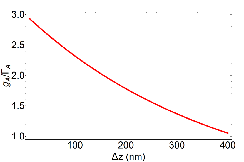
Fig.  S5: SC of SPs to both donors and acceptors. Ratio of SP collective coupling and linewidth of acceptors as a function of donor-acceptor separation $\Delta z$.

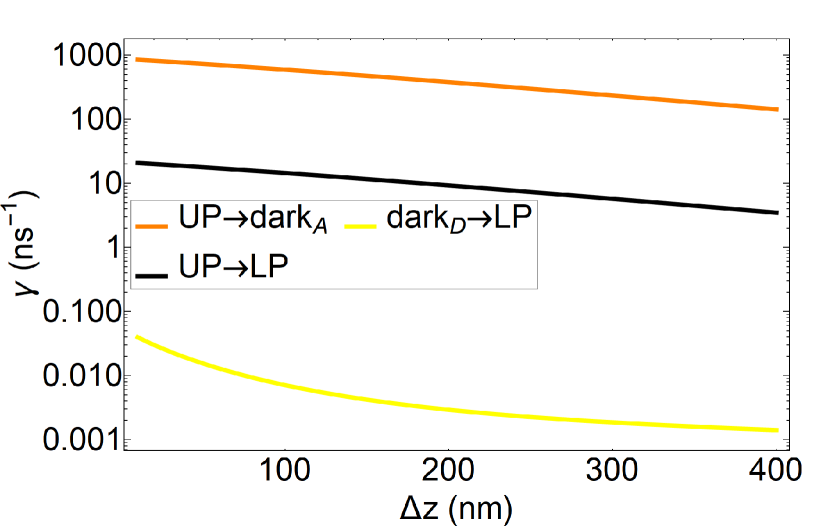
Fig.  S6: SC of SPs to both donors and acceptors. EET rates (that are not shown in Fig. 4 of the main text) as a function of donor-acceptor separation $\Delta z$ for downhill transtions among polariton and dark states. for The SP mode is resonant with the donor, and the donor slab lies 1 nm from the metal and has fixed position while the acceptor slab is moved in the $+z$-direction to vary $\Delta z$.

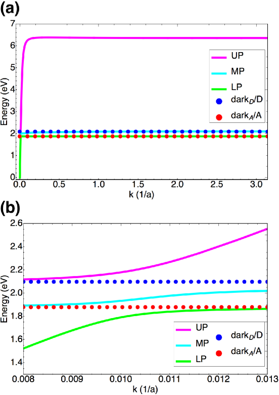
Fig.  S7: SC of SPs to both donors and acceptors. (a) Dispersion curve in the FBZ. Donor-acceptor separation is 205 nm. The dispersion curves at all other donor-acceptor separations (10-400 nm) have the same qualitative form. The value $a=1\times 10^{-9}\text{ m}$ is the inter-chromophoric lattice spacing for both donor and acceptor slabs. (b) Expanded view of dispersion curve at region of anticrossing characteristic of SC.

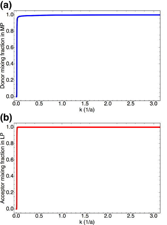
Fig.  S8: SC of SPs to both donors and acceptors. (a) Donor mixing fraction $|c_{D_{\vec{k}}\text{MP}_{\vec{k}}}|^{2}$ in MP and (b) acceptor mixing fraction $|c_{A_{\vec{k}}\text{LP}_{\vec{k}}}|^{2}$ in LP. Donor-acceptor separation is 205 nm. The mixing-fraction curves as a function of $\vec{k}\in\text{FBZ}$ at all other donor-acceptor separations have the same qualitative form. The value $a=1\times 10^{-9}\text{ m}$ is the inter-chromophoric lattice spacing for both donor and acceptor slabs.

References

- Govorov et al. 2016 A. Govorov, P. L. H. Martínez and H. V. Demir, Understanding and Modeling Förster-type Resonance Energy Transfer (FRET): Introduction to FRET, Springer Singapore, 2016.
- Jang et al. 2004 S. Jang, M. D. Newton and R. J. Silbey, Phys. Rev. Lett., 2004, 92, 218301.
- Jang et al. 2007 S. Jang, M. D. Newton and R. J. Silbey, J. Phys. Chem. B, 2007, 111, 6807–6814.
- Kassal et al. 2013 I. Kassal, J. Yuen-Zhou and S. Rahimi-Keshari, J. Phys. Chem. Lett., 2013, 4, 362–367.
- Lloyd and Mohseni 2010 S. Lloyd and M. Mohseni, New J. Phys., 2010, 12, 075020.
- Engel et al. 2007 G. S. Engel, T. R. Calhoun, E. L. Read, T.-K. Ahn, T. Mančal, Y.-C. Cheng, R. E. Blankenship and G. R. Fleming, Nature, 2007, 446, 782.
- Duque et al. 2015 S. Duque, P. Brumer and L. A. Pachón, Phys. Rev. Lett., 2015, 115, 110402.
- Scholes 2003 G. D. Scholes, Annu. Rev. Phys. Chem., 2003, 54, 57–87.
- Haedler et al. 2015 A. T. Haedler, K. Kreger, A. Issac, B. Wittmann, M. Kivala, N. Hammer, J. Kohler, H.-W. Schmidt and R. Hildner, Nature, 2015, 523, 196–199.
- Saikin et al. 2017 S. K. Saikin, M. A. Shakirov, C. Kreisbeck, U. Peskin, Y. N. Proshin and A. Aspuru-Guzik, The Journal of Physical Chemistry C, 2017, 121, 24994–25002.
- Hsu et al. 2017 L.-Y. Hsu, W. Ding and G. C. Schatz, J. Phys. Chem. Lett., 2017, 8, 2357–2367.
- Zhang et al. 2014 X. Zhang, C. A. Marocico, M. Lunz, V. A. Gerard, Y. K. Gunâko, V. Lesnyak, N. Gaponik, A. S. Susha, A. L. Rogach and A. L. Bradley, ACS Nano, 2014, 8, 1273–1283.
- Ding et al. 2017 W. Ding, L.-Y. Hsu and G. C. Schatz, J. Chem. Phys., 2017, 146, 064109.
- Bouchet et al. 2016 D. Bouchet, D. Cao, R. Carminati, Y. De Wilde and V. Krachmalnicoff, Phys. Rev. Lett., 2016, 116, 037401.
- de Torres et al. 2016 J. de Torres, P. Ferrand, G. Colas des Francs and J. Wenger, ACS Nano, 2016, 10, 3968–3976.
- Andrew and Barnes 2004 P. Andrew and W. L. Barnes, Science, 2004, 306, 1002–1005.
- Zhong et al. 2017 X. Zhong, T. Chervy, L. Zhang, A. Thomas, J. George, C. Genet, J. A. Hutchison and T. W. Ebbesen, Angew. Chem., Int. Ed., 2017, 56, 9034–9038.
- Coles et al. 2014 D. M. Coles, N. Somaschi, P. Michetti, C. Clark, P. G. Lagoudakis, P. G. Savvidis and D. G. Lidzey, Nat. Mater., 2014, 13, 712–719.
- Slootsky et al. 2014 M. Slootsky, X. Liu, V. M. Menon and S. R. Forrest, Phys. Rev. Lett., 2014, 112, 076401.
- Feist and García-Vidal 2015 J. Feist and F. J. García-Vidal, Phys. Rev. Lett., 2015, 114, 196402.
- Schachenmayer et al. 2015 J. Schachenmayer, C. Genes, E. Tignone and G. Pupillo, Phys. Rev. Lett., 2015, 114, 196403.
- Yuen-Zhou et al. 2016 J. Yuen-Zhou, S. K. Saikin, T. Zhu, M. C. Onbasli, C. A. Ross, V. Bulovic and M. A. Baldo, Nat. Commun., 2016, 7, year.
- Basko et al. 2000 D. M. Basko, F. Bassani, G. C. La Rocca and V. M. Agranovich, Phys. Rev. B, 2000, 62, 15962–15977.
- Walls and Milburn 1994 D. Walls and G. Milburn, Quantum Optics, Springer-Verlag, 1994.
- Waks and Sridharan 2010 E. Waks and D. Sridharan, Phys. Rev. A, 2010, 82, 043845.
- Yuen-Zhou et al. arXiv:1711.11213 J. Yuen-Zhou, S. K. Saikin and V. Menon, ArXiv e-prints, arXiv:1711.11213.
- Zhou et al. 2011 F. Zhou, Y. Liu and Z.-Y. Li, Opt. Lett., 2011, 36, 1969–1971.
- González-Tudela et al. 2013 A. González-Tudela, P. A. Huidobro, L. Martín-Moreno, C. Tejedor and F. J. García-Vidal, Phys. Rev. Lett., 2013, 110, 126801.
- Archambault et al. 2010 A. Archambault, F. Marquier, J.-J. Greffet and C. Arnold, Phys. Rev. B, 2010, 82, 035411.
- Martínez-Martínez et al. 2017 L. A. Martínez-Martínez, R. F. Ribeiro, J. A. Campos Gonzalez Angulo and J. Yuen-Zhou, ACS Photonics, 2017.
- Jang et al. 2002 S. Jang, Y. Jung and R. J. Silbey, Chem. Phys., 2002, 275, 319–332.
- Jang and Silbey 2003 S. Jang and R. J. Silbey, J. Chem. Phys., 2003, 118, 9312–9323.
- Ma and Cao 2015 J. Ma and J. Cao, J. Chem. Phys., 2015, 142, 094106.
- Baghbanzadeh and Kassal 2016 S. Baghbanzadeh and I. Kassal, Phys. Chem. Chem. Phys., 2016, 18, 7459–7467.
- Baghbanzadeh and Kassal 2016 S. Baghbanzadeh and I. Kassal, J. Phys. Chem. Lett., 2016, 7, 3804–3811.
- Mukamel 1995 S. Mukamel, Principles of nonlinear optical spectroscopy, Oxford University Press, 1995.
- Herrera and Spano 2016 F. Herrera and F. C. Spano, Phys. Rev. Lett., 2016, 116, 238301.
- Scholes et al. 2017 G. D. Scholes, G. R. Fleming, L. X. Chen, A. Aspuru-Guzik, A. Buchleitner, D. F. Coker, G. S. Engel, R. van Grondelle, A. Ishizaki, D. M. Jonas, J. S. Lundeen, J. K. McCusker, S. Mukamel, J. P. Ogilvie, A. Olaya-Castro, M. A. Ratner, F. C. Spano, K. B. Whaley and X. Zhu, Nature, 2017, 543, 647.
- Ozel et al. 2013 T. Ozel, P. L. Hernandez-Martinez, E. Mutlugun, O. Akin, S. Nizamoglu, I. O. Ozel, Q. Zhang, Q. Xiong and H. V. Demir, Nano Lett., 2013, 13, 3065–3072.
- Hutchison et al. 2012 J. A. Hutchison, T. Schwartz, C. Genet, E. Devaux and T. W. Ebbesen, Angew. Chem., Int. Ed., 2012, 51, 1592–1596.
- May and Kühn 2011 V. May and O. Kühn, Charge and Energy Transfer Dynamics in Molecular Systems, Wiley, 2011.
- Agranovich et al. 2003 V. M. Agranovich, M. Litinskaia and D. G. Lidzey, Phys. Rev. B, 2003, 67, 085311.
- Litinskaya et al. 2004 M. Litinskaya, P. Reineker and V. M. Agranovich, J. Lumin., 2004, 110, 364–372.
- del Pino et al. 2015 J. del Pino, J. Feist and F. J. Garcia-Vidal, New J. Phys., 2015, 17, 053040.
- Canaguier-Durand et al. 2015 A. Canaguier-Durand, C. Genet, A. Lambrecht, T. W. Ebbesen and S. Reynaud, Eur. Phys. J. D, 2015, 69, 24.
- Zhong et al. 2016 X. Zhong, T. Chervy, S. Wang, J. George, A. Thomas, J. A. Hutchison, E. Devaux, C. Genet and T. W. Ebbesen, Angew. Chem., Int. Ed., 2016, 55, 6202–6206.
- Palik 1985 E. Palik, Handbook of Optical Constants of Solids II, Academic Press, 1985.
- Bellessa et al. 2004 J. Bellessa, C. Bonnand, J. C. Plenet and J. Mugnier, Phys. Rev. Lett., 2004, 93, 036404.
- Ma et al. 2015 J. Ma, J. Moix and J. Cao, J. Chem. Phys., 2015, 142, 094107.
- Moix et al. 2015 J. M. Moix, J. Ma and J. Cao, J. Chem. Phys., 2015, 142, 094108.
- Valleau et al. 2012 S. Valleau, S. K. Saikin, M.-H. Yung and A. A. Guzik, J. Chem. Phys., 2012, 137, 034109.
- Govorov et al. 2007 A. O. Govorov, J. Lee and N. A. Kotov, Phys. Rev. B, 2007, 76, 125308.
- Valeur and Berberan-Santos 2012 B. Valeur and M. Berberan-Santos, Molecular Fluorescence: Principles and Applications, Wiley, 2nd edn., 2012.
- Medintz and Hildebrandt 2013 I. Medintz and N. Hildebrandt, FRET - Förster Resonance Energy Transfer: From Theory to Applications, Wiley, 2013.
- Dung et al. 2002 H. T. Dung, L. Knöll and D.-G. Welsch, Phys. Rev. A, 2002, 66, 063810.
- Coles et al. 2011 D. M. Coles, P. Michetti, C. Clark, W. C. Tsoi, A. M. Adawi, J.-S. Kim and D. G. Lidzey, Adv. Funct. Mater., 2011, 21, 3691–3696.
- Virgili et al. 2011 T. Virgili, D. Coles, A. M. Adawi, C. Clark, P. Michetti, S. K. Rajendran, D. Brida, D. Polli, G. Cerullo and D. G. Lidzey, Phys. Rev. B, 2011, 83, 245309.
- Coles et al. 2011 D. M. Coles, P. Michetti, C. Clark, A. M. Adawi and D. G. Lidzey, Phys. Rev. B, 2011, 84, 205214.
- Somaschi et al. 2011 N. Somaschi, L. Mouchliadis, D. Coles, I. E. Perakis, D. G. Lidzey, P. G. Lagoudakis and P. G. Savvidis, Appl. Phys. Lett., 2011, 99, 143303.
- Coles et al. 2013 D. M. Coles, R. T. Grant, D. G. Lidzey, C. Clark and P. G. Lagoudakis, Phys. Rev. B, 2013, 88, 121303.
- Chovan et al. 2008 J. Chovan, I. E. Perakis, S. Ceccarelli and D. G. Lidzey, Phys. Rev. B, 2008, 78, 045320.
- Michetti and La Rocca 2008 P. Michetti and G. C. La Rocca, Phys. Rev. B, 2008, 77, 195301.
- Michetti and La Rocca 2009 P. Michetti and G. C. La Rocca, Phys. Rev. B, 2009, 79, 035325.
- Lidzey et al. 2002 D. G. Lidzey, A. M. Fox, M. D. Rahn, M. S. Skolnick, V. M. Agranovich and S. Walker, Phys. Rev. B, 2002, 65, 195312.
- Skolnick et al. 1998 M. S. Skolnick, T. A. Fisher and D. M. Whittaker, Semicond. Sci. Technol., 1998, 13, 645.
- Holmes and Forrest 2007 R. J. Holmes and S. R. Forrest, Org. Electron., 2007, 8, 77–93.
- Törmä and Barnes 2015 P. Törmä and W. L. Barnes, Rep. Prog. Phys., 2015, 78, 013901.
- Garcia-Vidal and Feist 2017 F. J. Garcia-Vidal and J. Feist, Science, 2017, 357, 1357–1358.
- Kenkre and Reineker 1982 V. Kenkre and P. Reineker, Exciton Dynamics in Molecular Crystals and Aggregates, Springer-Verlag, 1982.
- Sarovar et al. 2010 M. Sarovar, A. Ishizaki, G. R. Fleming and K. B. Whaley, Nat. Phys., 2010, 6, 462–467.
- Galego et al. 2016 J. Galego, F. J. Garcia-Vidal and J. Feist, Nat. Commun., 2016, 7, 13841.
- Flick et al. 2017 J. Flick, M. Ruggenthaler, H. Appel and A. Rubio, Proc. Natl. Acad. Sci. U. S. A., 2017, 114, 3026–3034.
- 73 L. A. Martínez-Martínez, M. Du, R. F. Ribeiro, S. Kéna-Cohen and J. Yuen-Zhou, ArXiv e-prints, arXiv:1711.11264.
- Novotny and Hecht 2012 L. Novotny and B. Hecht, Principles of Nano-Optics, Cambridge University Press, 2nd edn., 2012.
- Sumi 1999 H. Sumi, J. Phys. Chem. B, 1999, 103, 252–260.
- Feshbach 1958 H. Feshbach, Ann. Phys., 1958, 5, 357–390.
- Feshbach 1962 H. Feshbach, Ann. Phys., 1962, 19, 287–313.
- Shapiro and Brumer 2012 M. Shapiro and P. Brumer, Quantum Control of Molecular Processes, Wiley, 2012.
- Cohen and Mukamel 2003 A. E. Cohen and S. Mukamel, J. Phys. Chem. A, 2003, 107, 3633–3638.