30th November 2017, arXiv:1711.11546

Revised version 28th February 2018

Accepted by Europ. Phys. J. A.

Comprehensive Study of Observables in Compton Scattering on the Nucleon

Harald W. Grießhammer^a, Judith A. McGovern^b and Daniel R. Phillips^c

^a Institute for Nuclear Studies, Department of Physics,
The George Washington University, Washington DC 20052, USA

^b School of Physics and Astronomy, The University of Manchester,
Manchester M13 9PL, UK

^c Department of Physics and Astronomy and Institute of Nuclear and Particle Physics, Ohio University, Athens, Ohio 45701, USA

We present an analysis of $13$ observables in Compton scattering on the proton. Cross sections, asymmetries with polarised beam and/or targets, and polarisation-transfer observables are investigated for energies up to the $\Delta(1232)$ resonance to determine their sensitivity to the proton’s dipole scalar and spin polarisabilities. The Chiral Effective Field Theory Compton amplitude we use is complete at N⁴LO, $\mathcal{O}(e^{2}\delta^{4})$, for photon energies $\omega\sim m_{\pi}$, and so has an accuracy of a few per cent there. At photon energies in the resonance region, it is complete at NLO, $\mathcal{O}(e^{2}\delta^{0})$, and so its accuracy there is about $20$%. We find that for energies from pion-production threshold to about $250\;\mathrm{MeV}$, multiple asymmetries have significant sensitivity to presently ill-determined combinations of proton spin polarisabilities. We also argue that the broad outcomes of this analysis will be replicated in complementary theoretical approaches, e.g., dispersion relations. Finally, we show that below the pion-production threshold, $6$ observables suffice to reconstruct the Compton amplitude, and above it $11$ are required. Although not necessary for polarisability extractions, this opens the possibility to perform “complete” Compton-scattering experiments. An interactive Mathematica notebook, including results for the neutron, is available from judith.mcgovern@manchester.ac.uk.

Suggested Keywords: Effective Field Theory, proton, neutron and nucleon polarisabilities, spin polarisabilities, Chiral Perturbation Theory, $\Delta(1232)$ resonance

1 Introduction

Compton scattering from a spin-$\frac{1}{2}$ target is fully described by six amplitudes, as first shown in ref. [1]. These are functions of the incoming photon energy $\omega$ and the photon scattering angle $\theta$; they become complex above the pion-production threshold. At sufficiently low energy, gauge and Lorentz invariance require that the process reduces to Thomson scattering, depending only on the charge and mass of the target. At somewhat higher energies, deviations become apparent. For nucleons, some deviations are explained by treating the target as a Dirac particle with an anomalous magnetic moment, and by including neutral pion exchange (the pion-pole contribution). Others are due to internal hadronic structure and excitations. The principal such effects at low energy are the nucleon’s electric and magnetic dipole polarisabilities, $\alpha_{E1}$ and $\beta_{M1}$. They reveal the extent to which charge and current distributions in the target shift under the influence of external electromagnetic fields and parametrise the strength of the induced radiation dipoles. Then, in the amplitudes that are sensitive to the target’s spin, four “spin polarisabilities” $\gamma_{i}$ govern the departure from point-like scattering and parametrise the response of the spin degrees of freedom. Each of these six low-energy parameters is as fundamental a property of the nucleon as its anomalous magnetic moment, and they are equally useful summaries of its composition. However, even for the proton, these $6$ numbers are not well determined: only one combination is known with better than 2% accuracy, while current uncertainties vary from 10% to over 100% for the rest. A rigorous test of our understanding of QCD will be provided by comparing lattice QCD computations of these parameters, the first of which are emerging (see ref. [2] for a recent compilation), with extractions from Compton data on the proton and light nuclear targets. This will be a new benchmark of our ability to use QCD to compute the proton’s structure.

However, a significant problem is that in the low-energy expansion which parametrises the amplitudes purely as “Born plus pion-pole plus polarisabilities”, the polarisabilities, especially the spin ones, have little effect below $\omega_{\mathrm{lab}}\approx 100$ MeV. And this expansion breaks down altogether as the pronounced cusp due to photoproduction is approached; see also fig. 1. Thus, the link between the amplitudes and their low-energy limits is lost entirely, unless one can resort to an underlying theoretical description of the process. In this paper, we describe the amplitudes using Chiral Effective Field Theory ($\chi$EFT), the effective field theory of nucleons and pions, in a variant which also includes the $\Delta(1232)$. $\chi$EFT is formulated as a perturbative expansion in the ratio of the photon energy and other small scales over the mass of omitted degrees of freedom such as the $\rho$ meson. $\chi$EFT amplitudes thus have a theoretical uncertainty that can be quantified from the truncation at a given order.

Contributions from short-distance structure can have a significant effect on $\chi$EFT’s predictions for polarisabilities. However, one can compare $\chi$EFT’s amplitudes with those of the complementary, dispersion-relation, approach [3] when common values of the $6$ polarisabilities are adopted. We make this comparison for moderate energies in sect. 2.3 and show that the heavier degrees of freedom omitted from the $\chi$EFT calculation have very little impact on the residual (beyond dipole polarisabilities) energy dependence of the Compton amplitudes there. Thus, we argue it makes sense to trust the $\chi$EFT energy dependence up to $\omega_{\mathrm{lab}}\approx 250\;\mathrm{MeV}$, while fitting the polarisabilities to Compton data. We then explore the sensitivity of observables to the polarisability values, arguing that those sensitivities should be rather independent of the theoretical approach we have adopted.

The world data set for unpolarised scattering on the proton between $50$ and $170\;\mathrm{MeV}$ is quite rich and was used to extract the scalar polarisabilities in the $\chi$EFT framework in ref. [4]. Very similar results were obtained in a related work [5] (see also ref. [6]). From $170$ to $250$ MeV, the data are sparse and not fully in agreement. Low-energy data on the deuteron also exist and have been used to extract the neutron’s scalar polarisabilities in ref. [7], albeit with larger statistical and theoretical uncertainties. More recently, attention has largely shifted to polarised scattering, in part with the goal of extracting one or more of the spin polarisabilities. Two recent publications from MAMI [8, 9] are a promising start, though, for reasons we will explain in sect. 2.3, from our perspective, only the second presents data at energies where a polarisability extraction is substantially free of theory uncertainties [10].

In a seminal paper, Babusci et al. [11] carried out a comprehensive study of the relationship between the $6$ Compton amplitudes and the $13$ observables which characterise scattering events in which at most one photon and at most one nucleon, in either the in or out states, is polarised. The primary observables are ratios of cross section differences for different orientations of a particle’s polarisation to sums of those same cross sections. If all polarised particles are incoming, these are termed asymmetries; if one is incoming and one outgoing, polarisation transfers. While measuring the polarisation of outgoing photons at these energies is impractical, recoil nucleon polarimetry is feasible: it has, for example, been done for photoproduction at MAMI. But there has, to date, been no study of the sensitivity of Compton polarisation-transfer reactions to nucleon polarisabilities. As for asymmetries, after initial studies for linear and circular photon polarisations by Hildebrandt et al. [12, 13], Pasquini et al. [14] explored their sensitivities to polarisabilities; indeed, this study was instrumental in motivating the MAMI experiments described in refs. [15, 8, 16, 17, 18]. Other partial studies have since been presented elsewhere [19, 20]. In this paper, we present a comprehensive analysis of the sensitivities of all $13$ observables to the $6$ polarisabilities. Furthermore, since two combinations of the polarisabilities can be deduced with considerable accuracy from total photoproduction cross sections, we are particularly interested in sensitivity to combinations that are orthogonal to those.

The observables and amplitudes presented in this paper are available via a Mathematica notebook from judith.mcgovern@manchester.ac.uk. It contains routines for cross-sections, rates and asymmetries from zero to about $340$ MeV in the lab frame and allows the scalar and spin polarisabilities to be varied. It also gives all observables for scattering on a free neutron target, for perusal in the context of few-nucleon experiments in quasi-free neutron kinematics.

The paper is organised as follows. In sect. 2, we briefly review the ingredients of our $\chi$EFT calculation of Compton scattering and list the pertinent observables. In sect. 3, we first discuss the magnitudes of the proton observables without adjusting the polarisabilities, and then present the sensitivities of those observables to changes in the polarisabilities. Finally, we provide selected results for the free neutron. Our conclusions are given in sect. 4. Our reference values of polarisabilities are provided and briefly discussed in appendix A, technical details on the observables can be found in appendix B, and comments on Babusci et al. [11] in appendix C. This last appendix includes a proof that the observables suffice to reconstruct the Compton amplitudes. A supplement studying the sensitivities of neutron observables is available online and as appendix D of the arXiv version.

2 Formalism

2.1 Definition of Polarisabilities

As discussed above, the polarisabilities characterise the low-energy response of the target to external electric and magnetic fields, $\vec{E}$ and $\vec{B}$. This can be described by the following effective Hamiltonian [11], which includes all terms that contribute up to order $\omega^{4}$ in the low-energy expansion:

$$\mathcal{H}_{\rm eff}^{(2)}= -\frac{1}{2}\,4\pi\left(\alpha_{E1}\vec{E}^{2}+\beta_{M1}\vec{B}^{2}\right.$$

$$+\gamma_{E1E1}\vec{\sigma}\cdot\vec{E}\times\dot{\vec{E}}+\gamma_{M1M1}\vec{\sigma}\cdot\vec{B}\times\dot{\vec{B}}-2\gamma_{M1E2}E_{ij}\sigma_{i}B_{j}+2\gamma_{E1M2}B_{ij}\sigma_{i}B_{j}$$

$$+\left.\alpha_{E1\nu}\dot{\vec{E}}^{2}+\beta_{M1\nu}\dot{\vec{B}}^{2}-\frac{1}{12}\,4\pi(\alpha_{E2}E_{ij}^{2}+\beta_{M2}B_{ij}^{2})\right)+\dots\;\;,$$ (2.1)

where $\vec{\sigma}$ is the nucleon spin operator and $T_{ij}=\frac{1}{2}(\nabla_{i}T_{j}+\nabla_{j}T_{i})$ with $T=E,B$. Here $\gamma_{i}$ are the four spin polarisabilities, labelled by the multipolarities of the incident and outgoing photon, $Xl\to X^{\prime}l^{\prime}$ with $l^{\prime}=l\pm\{0,1\}$. Accordingly, $\alpha_{E1}$, $\beta_{M1}$ and $\gamma_{i}$ are called dipole polarisabilities, while $\alpha_{E2}$ and $\beta_{M2}$ are quadrupole ones. The coefficients $\alpha_{E1\nu}$ and $\beta_{M1\nu}$ are “dispersive polarisabilities”: they contribute to the amplitudes in the same places and with the same angular dependence as $\alpha_{E1}$ and $\beta_{M1}$, but with an extra power of $\omega^{2}$. The expansion of $\mathcal{H}_{\rm eff}$—and of the Compton amplitude—in photon energies fails as the pion-production threshold is approached because of the non-analyticities that introduces. Another interpretation of eq. (2.1) is that it reproduces the first few terms of a multipole expansion of those parts of the Compton amplitude which go beyond the Powell amplitude, i.e. beyond that for a point target with an anomalous magnetic moment. This last interpretation is discussed further in sect. 2.3, with details presented in refs. [12, 21]. Finally, we mention that we quote $\alpha_{E1}$ and $\beta_{M1}$ in units of $10^{-4}\;\mathrm{fm}^{3}$, and the spin polarisabilities in units of $10^{-4}\;\mathrm{fm}^{4}$, throughout our presentation.

As stressed in refs. [11, 22], this non-relativistic Hamiltonian is frame-dependent and hence so is the definition of the polarisabilities; like those authors, we choose the Breit frame, which has the advantage over the centre-of-mass (cm) frame (used by ref. [23]) of being crossing-symmetric. The relation between the polarisabilities and the low-energy expansion of the Breit- or cm-frame amplitudes is given in eq. (B).

$\chi$EFT is summarised in the next section. It makes predictions based on pion-cloud and Delta-resonance effects for all of these polarisabilities; short-range effects enter the chiral expansion for a particular polarisability at an order which increases with every derivative in the effective Hamiltonian. This short-range nucleon structure—which is not resolved by $\chi$EFT—affects the $6$ polarisabilities under discussion here quite significantly, but its effect on the remaining energy dependence of the Compton amplitude occurs at a higher order in the chiral expansion. The dipole spin polarisabilities are, strictly speaking, predictions at the chiral order to which we work, but we allow them to vary in order to assess the ways in which they affect observables. Therefore, in sects. 3.5 and 3.6, we discuss the sensitivity of observables with respect to variations of the polarisabilities around the $\chi$EFT values quoted in appendix A, assuming that—at least for $\omega_{\mathrm{lab}}\lesssim 250$ MeV—the rest of the energy dependence of the Compton amplitude is correctly captured in $\chi$EFT. Such variation is, in fact, the method by which we determined the static polarisabilities $\alpha_{E1}$ and $\beta_{M1}$ (and gleaned some information on $\gamma_{M1M1}$) in our earlier fit to the proton Compton database [4]. It also means that we vary only the $6$ dipole polarisabilities $\alpha_{E1}$, $\beta_{M1}$ and $\gamma_{i}$, and not any higher polarisabilities. In fact, the entire contribution of $l\geq 2$ multipoles to the asymmetries has been shown to be small at the energies we examine here [13]. In addition, the chance of extracting coefficients from a sparse and noisy database in a statistically meaningful way decreases dramatically with multipolarity. We note that our polarisability-variation strategy concurrently provides an assessment of which kinematics and observables give complementary tests of the $\chi$EFT prediction for the Compton amplitude, since it shows places where that prediction is robust against changes in the specific values chosen for the dipole polarisabilities.

2.2 Compton Scattering on One Nucleon in $\chi$EFT

As the $\chi$EFT Compton amplitudes have been described in great detail in refs. [24, 4, 2], we refer to these for notation, the relevant parts of the chiral Lagrangian, and the pertinent amplitudes and parameters. Here, we only briefly recapitulate the main ingredients; full details are given in ref. [4]. Three typical low-energy scales exist in $\chi$EFT with a dynamical $\Delta(1232)$ degree of freedom: the pion mass $m_{\pi}$ as the typical chiral scale; the Delta-nucleon mass splitting $\Delta_{\scriptscriptstyle M}\approx 300\;\mathrm{MeV}$; and the photon energy $\omega$. Each provides a small, dimensionless expansion parameter when measured in units of a natural “high” scale $\Lambda_{\chi}\gg\Delta_{\scriptscriptstyle M},m_{\pi},\omega$ at which the theory is expected to break down because new degrees of freedom enter. While a three-parameter expansion is possible, it is more economical to follow Pascalutsa and Phillips [25] and take advantage of a convenient numerical coincidence by identifying

$$\delta\equiv\frac{\Delta_{M}}{\Lambda_{\chi}}\approx\left(\frac{m_{\pi}}{\Lambda_{\chi}}\right)^{1/2}\approx 0.4\ll 1\;\;.$$ (2.2)

For simplicity, we count $M_{\mathrm{N}}\sim\Lambda_{\chi}$ and employ one common breakdown scale $\Lambda_{\chi}\approx 650\;\mathrm{MeV}$, consistent with the masses of the $\omega$ and $\rho$ as the next-lightest exchange mesons. We can then identify two regimes of photon energy $\omega$ where the counting simplifies further [24, 4]. In regime I, $\omega\lesssim m_{\pi}$ counts like a chiral scale, $\omega\sim m_{\pi}\sim\delta^{2}\Lambda_{\chi}\ll\Delta_{M}$, and pion-cloud physics dominates. In contradistinction, in regime II, $\omega\sim\Delta_{M}\sim\delta^{1}\Lambda_{\chi}\gg m_{\pi}$, and the Delta resonance may be excited so that it strongly dominates the relevant channels and dwarfs contributions from the pion cloud through its large width and strong $\gamma\mathrm{N}\Delta$ coupling. Because of the increasing photon energy and the reordering of contributions expected around the Delta resonance, the level of theoretical uncertainty is actually different in these two regimes. The ingredients of our calculation ensure that the Compton amplitude contains in regime I all contributions at $\mathcal{O}(e^{2}\delta^{4})$ (N⁴LO, accuracy $\delta^{5}\approx 2\%$); and in regime II at $\mathcal{O}(e^{2}\delta^{0})$ (NLO, accuracy $\delta^{2}\approx 20\%$). For even higher energies, the expansion parameter approaches one, and the EFT series does not converge.

As detailed in ref. [4], the ingredients are covariant nucleon-Born, pion-pole and Delta-pole graphs, and heavy-baryon $\pi N$ and $\pi\Delta$ loop graphs to order $e^{2}\delta^{4}$ (i.e. chiral order $p^{4}$ plus leading Delta loops). The $\pi N$ loop corrections to the $\gamma N\Delta$ vertex are added to ensure Watson’s theorem is satisfied in photoproduction. These are higher order in regime I but NLO in regime II. Most physical constants that enter are taken from the Review of Particle Physics [26]; the $\gamma N\Delta$ coupling constants are close to those determined from photoproduction in ref. [27] but are adjusted slightly to fit the strength of the unpolarised differential Compton cross section at the Delta peak [4] (see also [28]). At ${\cal O}(e^{2}\delta^{4})$, there are two Compton-specific low-energy constants $\delta\alpha_{E1}$ and $\delta\beta_{M1}$ for each nucleon; these encode short-distance contributions to the scalar polarisabilities and have been fit to unpolarised Compton scattering data. To obtain a good description of this data, it was also necessary to fit $\gamma_{M1M1}^{(\mathrm{p})}$, though strictly speaking it is not a free parameter at this order; in this fit, the other spin polarisabilities were left at their predicted values.

For reference, we repeat (from ref. [2]) the $\chi$EFT values of the proton and neutron scalar and spin polarisabilities, together with their theoretical and (for extracted quantities) statistical errors, in appendix A. Table 1 of ref. [2] shows that, within the respective uncertainties, all values adopted here are compatible with those of other approaches and with available experimental information. And, in fact, while the exact results for rates and asymmetries depend on these particular values, we are more concerned here with the sensitivities of observables to polarisabilities; those are not markedly affected by the baseline polarisability values chosen. Those sensitivities should also be less dependent on details of the calculational framework used to compute them, as discussed in the Introduction and in sect. 2.3.

2.3 Comparing Theories via a Multipole Expansion

The basic output of this $\chi$EFT calculation is the $6$ energy- and angle-dependent amplitudes of eq. (B.1), and all observables are directly constructed from these. Any extraction of polarisabilities from experiment is only as good as the reliability of these amplitudes. We have already mentioned the fact that the power-counting provides an a priori estimate of theoretical uncertainties and indicates that they are intrinsically less reliable as the energy increases. However, even at low energies, other than the extent to which they have already been confronted with data [4, 7, 9], external validation is not easy. One important test, therefore, is the extent to which different approaches agree.

A useful summary is provided by the dynamical polarisabilities. They are the coefficients of the multipole expansion of the non-Born amplitudes in the cm frame at fixed energy, with a polynomial energy dependence divided out. At fixed photon energy, they are distinguished by different angular dependencies, and are single-variable functions of the photon energy. Dynamical polarisabilities were defined in refs. [29, 21] and further explained in refs. [12, 13, 22], so we will not repeat the definitions here. We do stress though that, as with any multipole expansion, they do not contain more information than the amplitudes themselves; it is just that the information is more readily accessible.

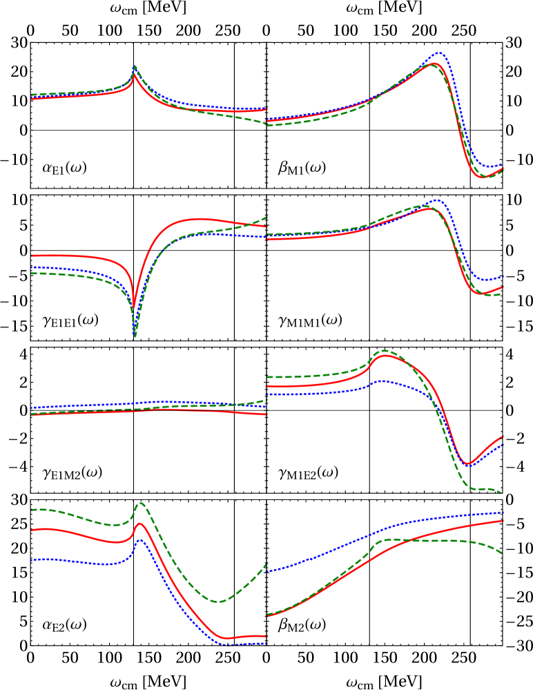
Figure 1: (Colour online) Real parts of the dominant dynamical polarisabilities for low-energy Compton scattering from the proton, plotted as a function of cm photon energy. The units are $10^{-4}\leavevmode\nobreak\ {\rm fm}^{n}$ where $n=3$ for $\alpha_{E1}$ and $\beta_{M1}$, $n=4$ for the $\gamma_{i}$, and $n=5$ for $\alpha_{E2}$ and $\beta_{E2}$. Red (solid): this work; green (dashed): DR-based by Pasquini et al. [21]; blue (dotted) 3rd-order covariant $\chi\mathrm{PT}$  by Lensky et al. [22]. Note that each row has its distinct plot scale.

For calculations and plots in the subsequent sections, we use the full amplitudes, and not the multipoles. But here, fig. 1 shows the first $8$ multipoles in the present theory (after fitting as described above), in the ${\cal O}(e^{2}\delta^{3})$ covariant framework of Lensky et al. [32, 22] (without fitting to data), and in the dispersion-relation framework of Pasquini et al. [3, 21, 33], based on integrals over pion-photoproduction multipoles (with $\alpha_{E1}-\beta_{M1}$ and $\gamma_{\pi}$ fit to Compton scattering data). We will compare these approaches shortly. The evolution of each dynamical polarisability with $\omega$ displays the relevant physics in each channel (cusps at the pion-production threshold, the Delta resonance, etc.). The value of a dynamical polarisability at $\omega=0$ is then the corresponding static polarisability. For the three sets of curves shown in fig. 1, these are the values tabulated in Table 1 of ref. [2] (see also [22]). Varying a static polarisability is identical to simply shifting the corresponding dynamical polarisability up or down.

As first noted in ref. [21], based on more limited results, there is a substantial degree of agreement on the shape of the polarisabilities up to around $250$ MeV lab energy ($200$ MeV cm energy in the figure). The same pion-loop and Delta-resonance physics is encoded in all three calculations. Furthermore, after adjusting the static polarisabilities to a common value, the results generically lie very close to one another. Indeed, they agree more closely than the theoretical error estimates shown in ref. [22] might suggest. In the Delta-dominated multipoles, this agreement continues up to surprisingly high energies, but overall disagreement creeps in above $250$ MeV lab energy, where one also expects polarisabilities beyond the dipole ones to play an increasing role. (The imaginary parts of the multipoles are much smaller than the real parts in this region, so we do not show them. They may actually be more easily accessible via pion photoproduction, see ref. [21]. For the Delta-dominated multipoles, for which the real parts vanish near the Delta pole, the imaginary parts agree well [22].)

It is important to remember that the units of the polarisabilities are not all the same. The large numerical factors in the definitions of $\alpha_{E2}$ and $\beta_{E2}$, and the dividing out of $\omega^{4}$ from these, conspire to make them look more important than they actually are, at least at low energies. Conversely, discrepancies between the polarisabilities are multiplied in the amplitudes by the appropriate powers of $\omega$, and hence are rather down-played by this depiction at high energies.

On the theory side, two main differences exist between the ingredients of this work and those of Lensky et al. [32, 22], which is also a $\chi$EFT calculation. First, in the latter, the pion loops are calculated in a kinematically-covariant framework. Second, their work is at ${\cal O}(e^{2}\delta^{3})$, i.e. one order lower than in ours. The most important physical consequence is that they, unlike us, omit the anomalous part of the magnetic moment of the nucleons in the pion-nucleon loops. Both differences imply that deviations between their approach and ours are indicative of the typical sizes of ${\cal O}(e^{2}\delta^{4})$ corrections (which are fully included in our approach).

A complementary approach is provided by dispersion relations [3] for the Compton amplitude, but these inherit uncertainties from the photoproduction database (which deteriorates at higher energies) and from the need to model the high-energy part of the dispersive integrals. Neither $\chi$EFT alone nor dispersion relations alone should be taken as the gold standard for the theory of Compton scattering. Rather, comparing the output of these two different approaches allows one to assess the reliability of each; where they agree, the results can confidently be described as framework-independent.

In ref. [8], data for $\Sigma_{2x}$ at a lab energy of approximately $300\;\mathrm{MeV}$ have been analysed in the dispersion-relation framework [3], and in Lensky’s covariant $\chi$EFT [32]. The results extracted for spin polarisabilities using the two theory approaches are consistent within the–somewhat sizeable—statistical uncertainties. However, the appreciable differences of their individual dynamical polarisabilities in fig. 1 at this energy suggest the similarity may mask rather different physics in the individual Compton amplitudes. From our perspective, therefore, this energy is too high to reliably conclude that polarisability extractions are framework-independent.

Thus, the message we take from fig. 1 is that there is a concurrence of theory approaches for the energy dependence of all $6$ dynamical polarisabilities up to around $250$ MeV lab energy. $\chi$EFT predictions of high intrinsic reliability only exist for energies up to a point not far beyond the pion-production threshold. However, up to $\omega_{\mathrm{lab}}\approx 250$ MeV, $\chi$EFT and dispersion relations agree quantitatively. We thus claim that there is an understanding of the energy dependence of dynamical polarisabilities in this energy domain which does not rely on the theoretical framework used. It is this range, therefore, on which we focus our attention when varying the polarisabilities. Planning of experiments then needs to balance the improved sensitivity to the polarisabilities at higher energies with the decreasing reliability of any extrapolation back to the zero-energy point.

2.4 Observables

We follow Babusci et al. [11] closely. The interested reader is directed to this invaluable resource for further details; some elucidation of certain subtleties in ref. [11] is given in appendix C.

We first define the kinematics and coordinate system. Unless otherwise specified, we work in the laboratory frame. The incident photon momentum is $\vec{k}$ ($|\vec{k}|=\omega_{\mathrm{lab}}$); the outgoing one is $\vec{k}^{\prime}$ ($|\vec{k}^{\prime}|=\omega^{\prime}_{\mathrm{lab}}=\omega_{\mathrm{lab}}/(1+\omega_{\mathrm{lab}}(1-\cos\theta)/M_{\mathrm{N}})$); the scattering angle $\theta$ is the angle between them, so $\vec{k}\cdot\vec{k}^{\prime}=\omega_{\mathrm{lab}}\,\omega^{\prime}_{\mathrm{lab}}\cos\theta$. As illustrated in fig. 2, the $z$-axis is defined as the incoming beam direction, $\vec{k}=k\;\vec{e}_{z}$; the scattering plane is the $xz$-plane, with the $y$-axis perpendicular to it to form a right-handed triplet, i.e. $\vec{k}\times\vec{k}^{\prime}=\omega_{\mathrm{lab}}\,\omega^{\prime}_{\mathrm{lab}}\sin\theta\;\vec{e}_{y}$. The angle from the scattering plane to the polarisation axis of a linearly-polarised photon is $\varphi_{\text{lin}}$. The nucleon recoils in the scattering plane; its momentum defines the $z^{\prime}$ axis; and a primed coordinate system $\{x^{\prime},y^{\prime},z^{\prime}\}$ is obtained from $\{x,y,z\}$ by a clockwise rotation through the recoil angle $\theta_{R}$ about the $y$ axis (which is also the $y^{\prime}$ axis).

For asymmetries with a polarised target, the target nucleon’s polarisation density is

$$\rho(P,\vec{n})=\frac{1}{2}\bigl{(}1+P\;\vec{\sigma}\cdot\vec{n}\bigr{)}$$ (2.3)

where $\vec{n}=(\sin\vartheta_{\vec{n}}\cos\varphi_{\vec{n}},\sin\vartheta_{\vec{n}}\sin\varphi_{\vec{n}},\cos\vartheta_{\vec{n}})$ ($|\vec{n}|=1$) is the nucleon spin direction, and $P\in[0;1]$ its degree of polarisation (Basel convention). We define the azimuthal angle $\vartheta_{\vec{n}}$ from the $z$-axis to $\vec{n}$ and polar angle $\varphi_{\vec{n}}$ from the $x$-axis to the projection of $\vec{n}$ onto the $xy$-plane; see fig. 2. For polarisation-transfer observables, it is customary to resolve the recoil polarisation direction $\vec{n}^{\prime}$ in the primed coordinate system, defining angles $\vartheta_{\vec{n}}^{\prime}$ and $\varphi_{\vec{n}}^{\prime}$ with respect to the $z^{\prime}$ axis and the scattering plane.

“Primed” indices are used to indicate the nucleon spin direction for polarisation-transfer observables, while unprimed ones are used for polarised targets. For example, $\Sigma_{y}$ is an asymmetry with the target nucleon polarised along the $y$ axis, while $\Sigma_{y^{\prime}}$ is a polarisation transfer observable from an unpolarised target to a recoil nucleon polarised along the $y^{\prime}$ direction.

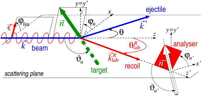
Figure 2: (Colour online) Kinematics and variables for polarisation asymmetries and polarisation-transfer observables.

The photon beam polarisation is characterised by the three Stokes parameters $\xi_{i}$, all of which satisfy $\xi_{i}\in[-1;1]$. $\xi_{2}$ is the degree of circular polarisation, with $\xi_{2}=\pm 1$ describing a fully right/left circularly polarised photon (positive/negative helicity); $\xi_{1}$ and $\xi_{3}$ describe linear polarisation with degree $\sqrt{\xi_{1}^{2}+\xi_{3}^{2}}\in[0;1]$ and polarisation angle specified by $\cos[2\varphi_{\text{lin}}]=\xi_{3}/\sqrt{\xi_{1}^{2}+\xi_{3}^{2}}$ and $\sin[2\varphi_{\text{lin}}]=\xi_{1}/\sqrt{\xi_{1}^{2}+\xi_{3}^{2}}$. Therefore, $\xi_{3}=\pm 1$ with $\xi_{1}=0$ describes a beam which is linearly polarised within/perpendicular to the scattering plane, and $\xi_{1}=\pm 1$ with $\xi_{3}=0$ one which is linearly polarised at angle $\varphi_{\text{lin}}=\pm\pi/4$ relative to the scattering plane.

With these definitions, Babusci et al. [11] parametrise the cross section with polarised beam and/or target and without detection of final-state polarisation as

$$\begin{split}\frac{\mathrm{d}\sigma}{\mathrm{d}\Omega}=\left.\frac{\mathrm{d}\sigma}{\mathrm{d}\Omega}\right|_{\text{unpol}}\;\bigg{[}1&\;+\;\xi_{3}\;\Sigma_{3}(\omega,\theta)\;+\;P\,n_{y}\;\Sigma_{y}(\omega,\theta)\;+\;P\,\xi_{1}\Big{(}n_{x}\;\Sigma_{1x}(\omega,\theta)+n_{z}\;\Sigma_{1z}(\omega,\theta)\Big{)}\\ &\;+\;P\,\xi_{2}\Big{(}n_{x}\;\Sigma_{2x}(\omega,\theta)+n_{z}\;\Sigma_{2z}(\omega,\theta)\Big{)}\;+\;P\,\xi_{3}\;n_{y}\;\Sigma_{3y}(\omega,\theta)\bigg{]}\;\;,\end{split}$$ (2.4)

where $n_{i}$ are the components of the polarisation vector $\vec{n}$ of the spin-$\frac{1}{2}$ target in its rest frame. This parametrisation can also be related to a more generally applicable one which uses spherical multipoles [34, 35].

The $8$ linearly independent asymmetries are:

• $1$ differential cross section $\displaystyle\left.\frac{\mathrm{d}\sigma}{\mathrm{d}\Omega}\right|_{\text{unpol}}$ of unpolarised photons on an unpolarised target.

• $1$ beam asymmetry of a linearly polarised beam on an unpolarised target:

  $$\Sigma_{3}=\frac{\mathrm{d}\sigma^{||}-\mathrm{d}\sigma^{\perp}}{\mathrm{d}\sigma^{||}+\mathrm{d}\sigma^{\perp}}\;\;.$$ (2.5)

  Here and below, $\mathrm{d}\sigma$ is shorthand for ${\mathrm{d}\sigma}/{\mathrm{d}\Omega}$; superscripts refer to photon polarisations (“$\parallel$” for polarisation in the scattering plane, “$\perp$” for perpendicular to it); subscripts to nucleon polarisations; and the absence of either means unpolarised.

• $1$ target asymmetry for nucleons polarised out of the scattering plane along the $\pm y$ direction and an unpolarised beam:

  $$\Sigma_{y}=\frac{\mathrm{d}\sigma_{y}-\mathrm{d}\sigma_{-y}}{\mathrm{d}\sigma_{y}+\mathrm{d}\sigma_{-y}}\;\;.$$ (2.6)

• $2$ double asymmetries of right/left-circularly polarised photons on a target polarised along the $\pm x$ or $\pm z$ directions:

  $$\Sigma_{2x}=\frac{\mathrm{d}\sigma^{R}_{x}-\mathrm{d}\sigma^{L}_{x}}{\mathrm{d}\sigma^{R}_{x}+\mathrm{d}\sigma^{L}_{x}}\;\;,\;\;\Sigma_{2z}=\frac{\mathrm{d}\sigma^{R}_{z}-\mathrm{d}\sigma^{L}_{z}}{\mathrm{d}\sigma^{R}_{z}+\mathrm{d}\sigma^{L}_{z}}\;\;.$$ (2.7)

• $3$ double asymmetries of linearly-polarised photons on a polarised target:

  $$\Sigma_{1x} =\frac{\mathrm{d}\sigma^{\pi/4}_{x}-\mathrm{d}\sigma^{-\pi/4}_{x}}{\mathrm{d}\sigma^{\pi/4}_{x}+\mathrm{d}\sigma^{-\pi/4}_{x}}\;\;,\;\;\Sigma_{1z}=\frac{\mathrm{d}\sigma^{\pi/4}_{z}-\mathrm{d}\sigma^{-\pi/4}_{z}}{\mathrm{d}\sigma^{\pi/4}_{z}+\mathrm{d}\sigma^{-\pi/4}_{z}}$$ (2.8)

  $$\Sigma_{3y} =\frac{(\mathrm{d}\sigma^{||}_{y}-\mathrm{d}\sigma^{\perp}_{y})-(\mathrm{d}\sigma^{||}_{-y}-\mathrm{d}\sigma^{\perp}_{-y})}{\mathrm{d}\sigma^{||}_{y}+\mathrm{d}\sigma^{\perp}_{y}+\mathrm{d}\sigma^{||}_{-y}+\mathrm{d}\sigma^{\perp}_{-y}}\;\;.$$ (2.9)

The decomposition of eq. (2.4) holds in both the lab and centre-of-mass frames, but the functions are frame-dependent. By time-reversal invariance, the $8$ recoil polarisations $\Sigma_{1^{\prime}x^{\prime}}$ etc. are related (but usually not identical) to the functions above.

Turning to polarisation-transfer observables, final-state photon polarisation is very hard to detect in the energy range of interest. Thus, we concentrate on those observables in which a polarised photon beam transfers its polarisation to a recoil nucleon, with an unpolarised target and undetected scattered-photon polarisation. (Polarisation transfer from a polarised target to a polarised scattered photon follows from time-reversal invariance.) The kinetic energy of the recoil nucleon increases near-linearly as a function of $\cos\theta$ from zero at $\theta=0^{\circ}$ to a maximum at $\theta=180^{\circ}$. The maximum recoil kinetic energy is $18\;\mathrm{MeV}$ for $\omega_{\mathrm{lab}}=100\;\mathrm{MeV}$ and $62\;\mathrm{MeV}$ at $\omega_{\mathrm{lab}}=200\;\mathrm{MeV}$. In polarisation transfer to the nucleon, an ideal experiment places an analyser in front of the detector to allow only certain recoil polarisations to be detected. Actual experiments use polarisation-dependent scattering, e.g., from ⁴He or ¹²C [36, 37].

Polarisation-transfer observables are defined by a parametrisation of the cross section very similar to that of eq. (2.4), but with the target polarisation axis $(\vartheta_{n},\varphi_{n})$ replaced by the orientation of the axis of the ideal analyser ($P^{\prime}\equiv 1$), with $(\vartheta_{\vec{n}}^{\prime},\varphi_{\vec{n}}^{\prime})$ measured in the “primed” coordinate system specified above:

$$\begin{split}\frac{\mathrm{d}\sigma}{\mathrm{d}\Omega}=\left.\frac{1}{2}\;\frac{\mathrm{d}\sigma}{\mathrm{d}\Omega}\right|_{\text{unpol}}\;\bigg{[}1&\;+\;n_{y^{\prime}}\;\Sigma_{y^{\prime}}(\omega,\theta)\;+\;\xi_{3}\;\Sigma_{3}(\omega,\theta)\;+\;\xi_{1}\Big{(}n_{x^{\prime}}\;\Sigma_{1x^{\prime}}(\omega,\theta)+n_{z^{\prime}}\;\Sigma_{1z^{\prime}}(\omega,\theta)\Big{)}\\ &\;+\;\xi_{2}\Big{(}n_{x^{\prime}}\;\Sigma_{2x^{\prime}}(\omega,\theta)+n_{z^{\prime}}\;\Sigma_{2z^{\prime}}(\omega,\theta)\Big{)}\;+\;\xi_{3}\;n_{y^{\prime}}\;\Sigma_{3y^{\prime}}(\omega,\theta)\bigg{]}\;\;.\end{split}$$ (2.10)

The overall factor of $\frac{1}{2}$ arises from the fact that, as we specify the final nucleon polarisation, we are no longer summing over final states. Of the $6$ extra functions introduced here, $\Sigma_{y^{\prime}}$ is equal to $\Sigma_{y}$ by time-reversal invariance, so there are $5$ new ones:

• $\Sigma_{2x^{\prime}}$ and $\Sigma_{2z^{\prime}}$ are polarisation transfers from circularly-polarised photons to a polarised recoiling nucleon;

• $\Sigma_{1x^{\prime}}$, $\Sigma_{1z^{\prime}}$ and $\Sigma_{3y^{\prime}}$ are polarisation transfers from linearly-polarised photons to a polarised recoiling nucleon.

Their definitions exactly follow eqs. (2.8), (2.7) and (2.9), but with the target spin labels $\{x,y,z\}$ replaced by $\{x^{\prime},y^{\prime},z^{\prime}\}$ and now referring to the analyser orientation $\vec{n}^{\prime}$ in the primed coordinate frame.

Only $6$ of the $13$ distinct observables are non-zero below the first strong inelasticity, which is set by the pion-production threshold: the cross section, the three asymmetries $\Sigma_{3}$, $\Sigma_{2x}$, $\Sigma_{2z}$, and the two polarisation-transfer observables $\Sigma_{2x^{\prime}}$ and $\Sigma_{2z^{\prime}}$. These suffice to determine the $6$ real Compton amplitudes $A_{i}$. Above threshold, these combine with any $5$ of the additional $7$ observables to provide all information on the $11$ independent real functions ($12$ minus an overall phase) of the complex Compton amplitudes. We prove this in appendix C.2.

This reconstruction could potentially provide valuable information on Compton amplitudes—in the same way that complete photoproduction experiments enhance our understanding of meson photoproduction. Complete low-energy Compton experiments would allow the extraction of polarisabilities from experiments at a single angle with no other theoretical biases, though the implementation of this approach may be some way off. They may prove to be more interesting at high energies, where the multipole expansion breaks down and the full amplitude needs to be reconstructed.

But this is not the type of experiment we focus on here. Instead, in what follows, we present the sensitivity of observables to the leading structure effects in the proton Compton amplitude, as encoded by the static dipole polarisabilities, with the goal of identifying a diverse set of observables, over a range of energies and angles, that together can provide constraints on those polarisabilities.

3 Results

We now present results for the $13$ observables defined in the previous section. These are given as contour plots, presentational details of which we explain in sects. 3.1 and 3.4. The plots in sects. 3.2 and 3.3 concern magnitudes of observables, while sects. 3.5 and 3.6 show sensitivities of observables to variations in the dipole scalar and spin polarisabilities (“sensitivity plots”). Unless otherwise stated, the kinematics are for Compton scattering on a proton in the lab frame (with the obvious exception being in sect. 3.7, where results for the neutron are presented), and the baseline values for polarisabilities are those given in appendix A. Before continuing, we reiterate that in all subsequent figures, we use the full Compton amplitudes, and not a truncated multipole expansion.

3.1 A Note on Contour Plots

We first discuss contour plots as a quick and intuitive way to assess both magnitudes of observables and their sensitivity to polarisabilities. A detailed analysis and extraction will of course need a more thorough comparison.

In all plots, we use a “heat scale” colour gradient, from deep blue to deep red. Except for the unpolarised cross section, deep blue indicates large and negative, while deep red is large and positive. The white region indicating “numerical zero” separates regions of small sensitivities, i.e. slightly blue and yellow tints. For asymmetries and polarisation-transfer observables, the extreme values of $1$ and $-1$ set the range naturally. For sensitivities, a common range was chosen by hand to maximise the information conveyed across all plots.

In fig. 3, we use the asymmetry $\Sigma_{2x}$ as an example of how a contour plot translates into transects along lines of constant photon energy or scattering angle. In it, a transect at $\omega_{\mathrm{lab}}=100\;\mathrm{MeV}$ is red and to the left, one at $\omega_{\mathrm{lab}}=200\;\mathrm{MeV}$ black and to the right. The transect at $\theta=70^{\circ}$ is at the bottom of the contour plot and colour-coded blue, and the one at $\theta=110^{\circ}$ is at the top and in green. They are chosen to be two of the angles at which MAMI has published data [15, 8]; the width of the energy bin is indicated as well. The coloured bands shown in these one-dimensional transects reproduce the heat scale used in the two-dimensional contour plot.

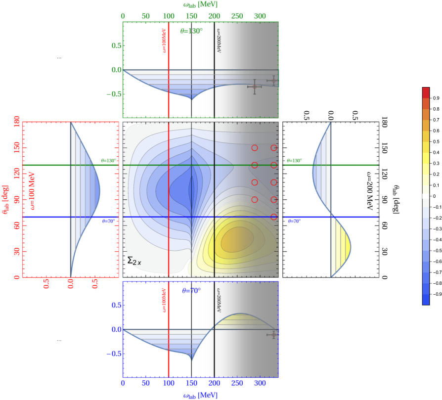
Figure 3: (Colour online) Illustration of a contour plot: the asymmetry $\Sigma_{2x}$, with transects at fixed $\omega_{\mathrm{lab}}=100\;\mathrm{MeV}$ (left, red), $\omega_{\mathrm{lab}}=200\;\mathrm{MeV}$ (right, black), $\theta=70^{\circ}$ (bottom, blue) and $\theta=110^{\circ}$ (top, green), and MAMI data [15, 8] added as open (red) circles. In the central plot, the size of the circles reflects neither data uncertainties, nor the size of the energy or angle bins. In the transects, statistical and systematic uncertainties, added in quadrature, are indicated, as is the width of the energy bins. Further comments in the text.

In the constant-angle transects and contour plots, the one-pion production threshold at $\omega_{\mathrm{lab}}^{\pi}=149.95\;\mathrm{MeV}$ is marked: the cusp there can also usually be discerned. For observables which are zero below this first inelasticity, the contour plot is shaded grey for $\omega_{\mathrm{lab}}<\omega_{\mathrm{lab}}^{\pi}$. Plots also indicate the energies and angles where data is available (without experimental uncertainties), so that regions which are already explored experimentally can be quickly identified. We have, however, not attempted to judge data quality. As it happens, the transects in fig. 3 reveal that the agreement between the $\chi$EFT prediction and the published MAMI data [15, 8] is quite good.

Finally, the figures also indicate the reliability of our predictions. As discussed in sect. 2.2, the $\chi$EFT expansion in momenta can systematically be improved but always becomes gradually less accurate with increasing photon energy. A more extensive discussion of these features and a less-handwaving, statistical interpretation using Bayesian degrees of belief can be found in refs. [2] and [4]. Here, we pragmatically indicate the fact demonstrated in sect. 2.3 that predictions from the two $\chi$EFT variants and from dispersion relations agree less well at higher energies by putting a grey mist over the colours in the contour plots. The grey mist begins to roll in at $\omega_{\mathrm{lab}}\gtrsim 200\;\mathrm{MeV}$, and makes things opaque above about $300\;\mathrm{MeV}$. In fig. 3, this indicates the MAMI data on $\Sigma_{2x}$ are in a region where polarisabilities cannot be extracted with high confidence.

There could be an exception to this trend of lower accuracy at higher energy. Since we tuned the parameters to reproduce the Delta peak, incorporated its width and made sure Watson’s theorem is approximately satisfied, we surmise that observables which are Delta-dominated are somewhat more reliable than the discussion in sect. 2.3 would suggest. The sensitivity of Delta-dominated observables to polarisability variations may thus perhaps be reliably predicted. However, there could be a similar degree of sensitivity to omitted physics: that would render polarisability extractions problematic. We also note that plots of most observables reveal quite a simple angular dependence at high energies. Given the limited accuracy of data at higher energies, different fits which each have just a few parameters but use different theoretical descriptions of the amplitudes may compare equally well with data there, but correspond to quite different static polarisability values.

3.2 Cross Section

Figure 4 is a contour plot of the differential cross section for Compton scattering on a proton, with contours on a logarithmic scale. As is well-known, below $140\;\mathrm{MeV}$ the cross section is rather flat, staying between $10$ and $20$ $\mathrm{nb/sr}$ except at forward angles. The cusp at the pion-production threshold is prominent for forward scattering, where the cross section decreases to less than $2\;\mathrm{nb/sr}$ at the threshold, but is hard to see for back angles. At higher energies, the broad width of the $\Delta(1232)$ resonance leads to a rapid increase by about two orders of magnitude. The maximum around $320\;\mathrm{MeV}$ is most pronounced at forward angles, where the cross section exceeds $400\;\mathrm{nb/sr}$, but it still reaches $170\;\mathrm{nb/sr}$ at backward angles.

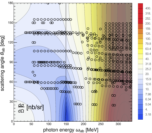
Figure 4: (Colour online) Contour plot of the unpolarised differential cross section as a function of $\omega_{\mathrm{lab}}$ and $\theta$, on a logarithmic scale, and with additional contours for very small and very large values. The colour coding is unique to this plot. The location of extant data is also indicated.

In refs. [24, 4], the world proton Compton database is listed and discussed extensively. Below 170 MeV, a few very old data sets as well as a small number of individual points must be discarded to obtain a statistically-consistent database. Above about $150\;\mathrm{MeV}$, data sets of purported high-precision experiments from different labs appear incompatible, and one is forced to choose the more copious set over the others in order to obtain a database for which the standard likelihood is a meaningful objective function. The result is that between $\omega_{\mathrm{lab}}=164$ MeV and $250\;\mathrm{MeV}$, the remaining data is very sparse and confined to only a couple of angles. This data gap is not, however, immediately apparent in plots such as fig. 4 because there the data are shown as black circles, without discriminating between experiments or indicating their quality. One can hence not discern all regions of poor kinematic coverage, but only those where data is completely absent. More details on the cross-section database, as well as comparisons with our $\chi$EFT results, can be found in ref. [4].

Lastly, we note that data has recently been taken on the differential cross section at $\omega_{\mathrm{lab}}\approx 85$ MeV at three different scattering angles at HI$\gamma$S and is presently being analysed [38].

3.3 Magnitudes of Asymmetries and Polarisation-Transfer Observables

In fig. 5, all $12$ asymmetries and polarisation-transfer observables are shown, with symbols at the energies and angles of available data: for $\Sigma_{3}$ from LEGS [39], MAMI [9] and MAMI (preliminary) [16, 18]; and from MAMI for $\Sigma_{2x}$ [15, 8] and $\Sigma_{2z}$ (preliminary) [18]. As in the case of the cross section, the symbols do not indicate data quality or statistical consistency. We also mention that recent HI$\gamma$S data on $\Sigma_{3}$ at $85\;\mathrm{MeV}$ is being analysed [38].

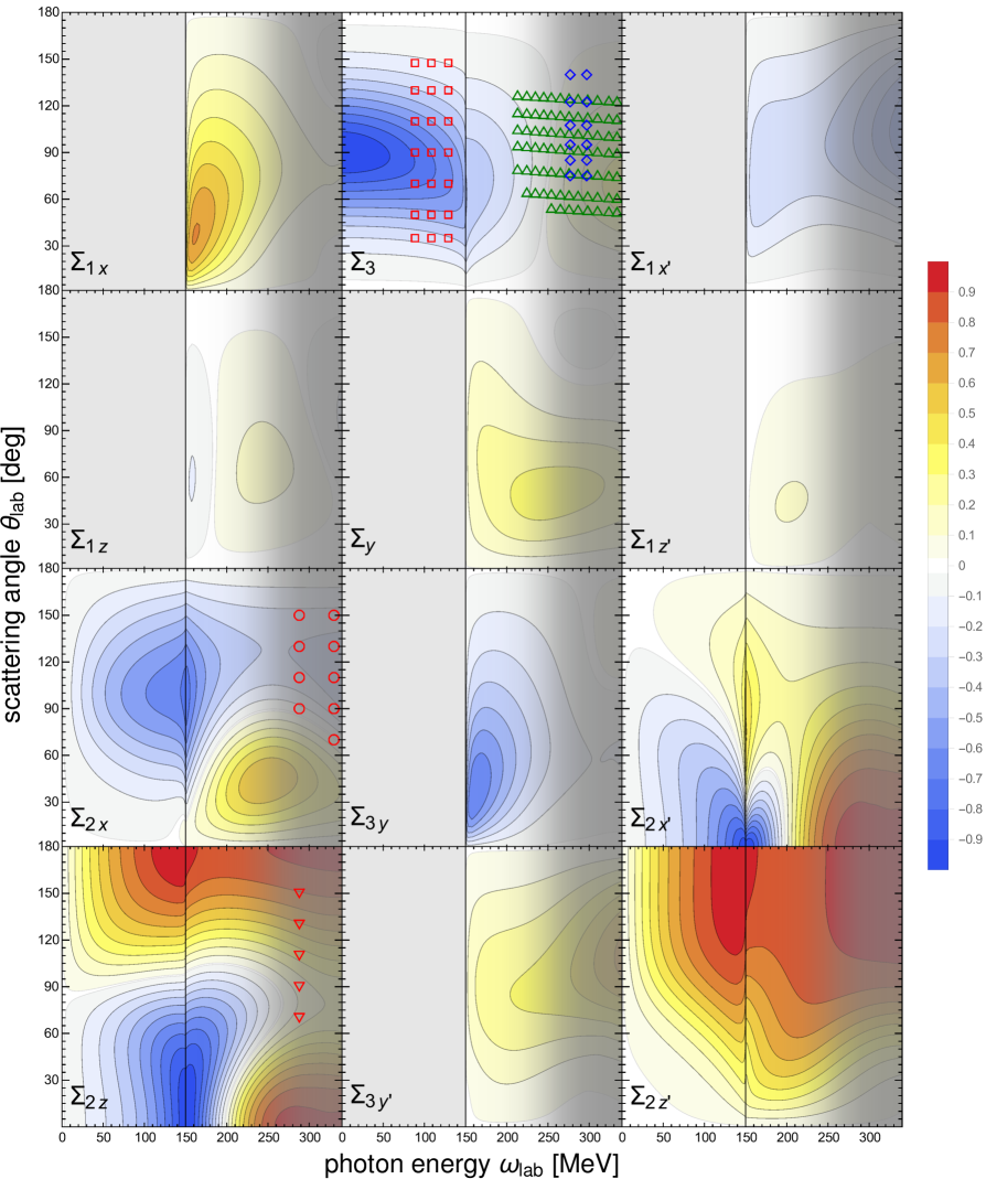
Figure 5: (Colour online) Contour plots of the asymmetries and polarisation-transfer observables; see text and sect. 3.1 for details. Data included as available, for $\Sigma_{3}$: open (green) triangles ${\color[rgb]{0.,0.7,0.}\bm{\bigtriangleup}}$ from LEGS [39], open (red) squares ${\color[rgb]{1,0,0}\bm{\square}}$ from MAMI [9], open (blue) diamonds

${\color[rgb]{0.,0.,1.0}\bm{\square}}$

preliminary from MAMI [16, 18]; for $\Sigma_{2x}$: open (red) circles ${\color[rgb]{1,0,0}\bm{\circ}}$ MAMI data from [15, 8]; open (red) inverted triangle ${\color[rgb]{1,0,0}\bm{\bigtriangledown}}$ preliminary from MAMI [18]. Symbol sizes do not reflect error bars, nor the size of energy or angle bins.

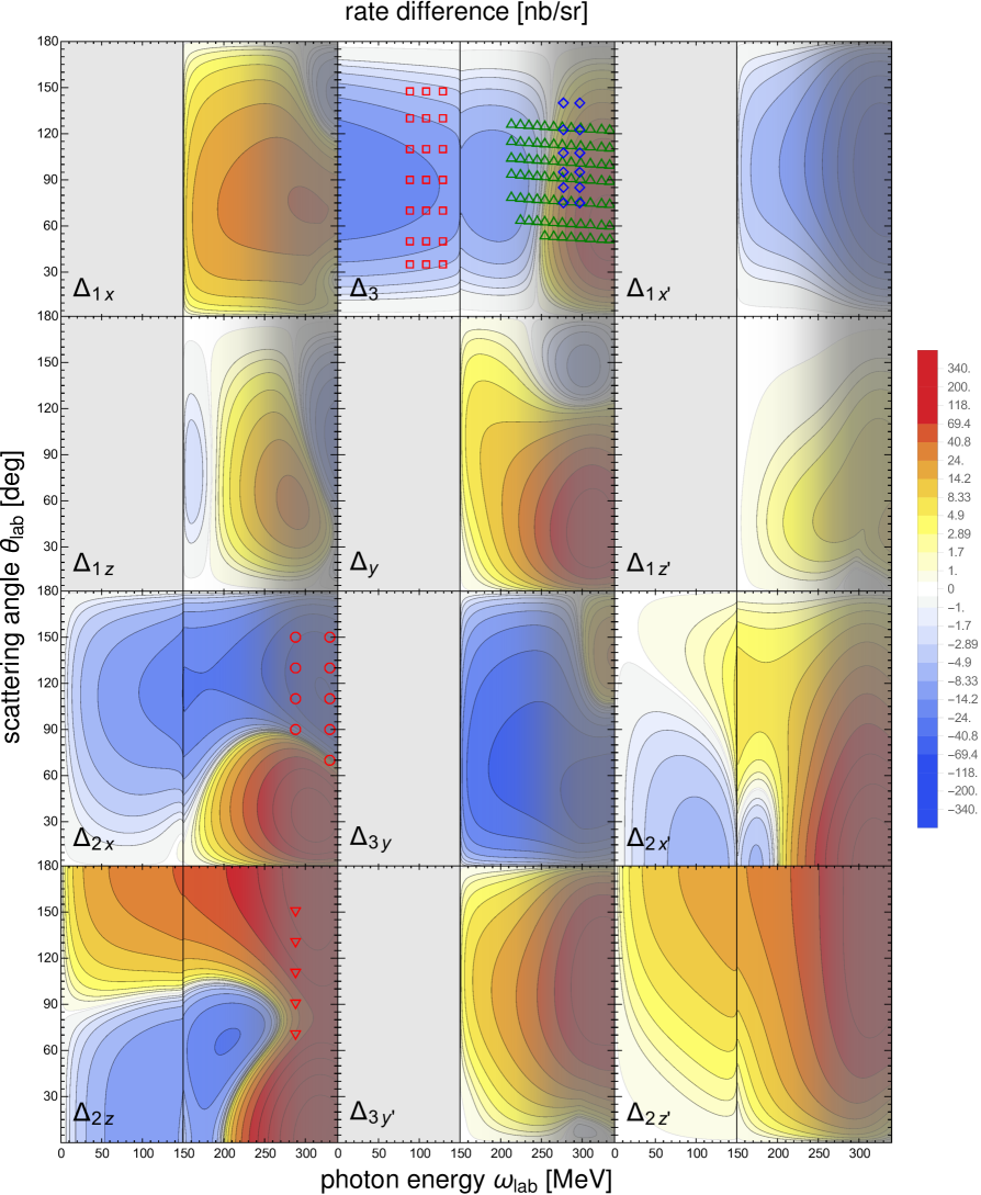
Figure 6: (Colour online) Contour plots of the rates associated with asymmetries and polarisation-transfer observables, with a unique colour coding on a logarithmic scale and additional contours for very small and very large values; see text for details. Data symbols as in fig. 5; their sizes do not reflect errors bars, nor the size of energy or angle bins.

It is worth pointing out that most of the observables are guaranteed to vanish at $\theta=0^{\circ}$ and $180^{\circ}$; the exceptions are $\Sigma_{2z}$, $\Sigma_{2x^{\prime}}$ and $\Sigma_{2z^{\prime}}$, with the last two vanishing at $\theta=180^{\circ}$ and $0^{\circ}$, respectively. When these observables do not vanish at $\theta=0^{\circ}$ or $180^{\circ}$, their contours meet the top and bottom of the frame at right angles. $\Sigma_{2z}$, $\Sigma_{2x^{\prime}}$ and $\Sigma_{2z^{\prime}}$ also tend to have the largest magnitudes, reaching $0.7$ in regions that are experimentally accessible.

The only asymmetry which does not vanish as the photon energy tends to zero is the beam asymmetry $\Sigma_{3}$. Its exact shape at zero energy is dictated by the Thomson term; this scattering on a point target without spin effects leads to a $(1-\cos^{2}\theta)/(1+\cos^{2}\theta)$ shape which is well-known from classical electrodynamics [40]. This behaviour dominates at low energies, although its importance has decreased dramatically by the pion-production threshold, with $\Sigma_{3}$ even changing sign above about $240\;\mathrm{MeV}$. It will turn out that $\Sigma_{3}$ has limited sensitivity to any polarisability at the energies where $\chi$EFT can be trusted to converge. Additional plots which compare to data can be found in ref. [9].

In general, all the observables which do not vanish below pion-production threshold are strongly driven by the Born and pion-pole amplitude at low energies, with small contributions from polarisabilities. At higher energies, all asymmetries are driven to a large degree by structure, namely pion-cloud, Delta-resonance and short-distance physics. Those observables which vanish below the pion-production threshold increase to magnitudes of at least $0.2$ for some angles around $200\;\mathrm{MeV}$ and thus can provide reasonable count rates there.

To facilitate run-time estimates, fig. 6 provides the differences of the rates, $\Delta_{\alpha}$, for different orientations associated with each asymmetry or polarisation-transfer observable, using colour coding on a logarithmic scale. These are the numerators in eqs. (2.5) to (2.9) for the asymmetries, and their analogues for polarisation transfers, for instance $\Delta_{3}=2\,\frac{\mathrm{d}\sigma}{\mathrm{d}\Omega}\,\Sigma_{3}$; see eq. (B.8) and appendix B for details.

3.4 General Comments on Sensitivities to Polarisabilities

After these plots of the $13$ observables with all values of the polarisabilities fixed, figs. 7 to 20 display the sensitivity of each observable $\mathcal{O}$ to varying individual polarisabilities, measured by the derivative

$$\frac{\mathrm{d}\mathcal{O}}{\mathrm{d}\zeta}$$ (3.1)

with respect to one of the $6$ polarisabilities, generically denoted $\zeta$. This corresponds to the effect of a change of static polarisability values (or, equivalently, of shifting a dynamical polarisability in fig. 1 up or down by a constant amount). In all such plots, we use the same heat scale as described in sect. 3.1. This allows one to quickly identify large sensitivities. Where necessary, more contours are added to display sensitivities beyond the extremes of the colour scale.

In what follows, our focus is on the region where three essential conditions are met: there are significant sensitivities to spin polarisabilities (usually $\omega_{\mathrm{lab}}\gtrsim 100\;\mathrm{MeV}$); theoretical frameworks can extract polarisabilities reliably and with high accuracy ($\omega_{\mathrm{lab}}\lesssim 250\;\mathrm{MeV}$); and experiments are not overwhelmed by backgrounds ($30^{\circ}\lesssim\theta\lesssim 160^{\circ}$).

In a brave new world of high-accuracy experiments with well-controlled systematic experimental uncertainties, high luminosities and 100% beam and target polarisations, an ideal observable should be very sensitive to one polarisability or a simple combination, while being rather insensitive to all others. Unfortunately, these plots show that one-nucleon Compton scattering does not admit such a simple picture. Spin polarisabilities will need to be extracted from a global analysis of a carefully selected set of observables. Redundancies can be built into this process, so as to ameliorate experimental and extraction uncertainties.

We therefore also explore sensitivities to particular linear combinations of polarisabilities. So long as data is incomplete, it is likely that any fit of polarisabilities to polarised cross sections and asymmetries will need to take advantage of the two famous sum rules for $\alpha_{E1}+\beta_{M1}$ and $\gamma_{0}$ which are based on total photoabsorption cross sections. The Baldin sum rule constrains $\alpha_{E1}+\beta_{M1}$ and has been evaluated most recently to give $14.0\pm 0.2$ [41]. The sum rule for the spin-dependent amplitude constrains the combination $\gamma_{0}$ of spin polarisabilities encountered under forward angles, and the most recent evaluation gives $0.93\pm 0.1$ [42]. Both numbers are in good agreement with, but more precise than, earlier evaluations [43, 44, 8].

Our plots confirm that the sensitivity to $\alpha_{E1}+\beta_{M1}$ dominates forward scattering, and that $\alpha_{E1}-\beta_{M1}$ can best be measured at back-angles. The difference, unlike the sum which is known to $1.5\%$, carries a combined theory and statistical uncertainty of greater than 10%. Errors of the spin polarisability combinations are greater than 20%; see ref. [2]. Overall, the sensitivities to scalar polarisabilities extend to lower energies than for the spin ones. In turn, an extraction of spin polarisabilities must also address uncertainties induced by the errors in the scalar ones. In particular at low energies, where the Born amplitudes are large and the scalar polarisabilities are the dominant deviation from Born, the sensitivity to $\alpha_{E1}-\beta_{M1}$ cannot be ignored when discussing the potential for spin-polarisability extractions. New experimental information at $\omega_{\mathrm{lab}}\lesssim 140\;\mathrm{MeV}$ can thus play a valuable—if indirect—role in reducing uncertainties in spin polarisabilities that are induced by the present error bars on $\alpha_{E1}$ and $\beta_{M1}$.

Likewise, the two combinations

$$\gamma_{0}:=-\gamma_{E1E1}-\gamma_{M1M1}-\gamma_{E1M2}-\gamma_{M1E2}\;\;,\;\;\gamma_{\pi}:=-\gamma_{E1E1}+\gamma_{M1M1}-\gamma_{E1M2}+\gamma_{M1E2}$$ (3.2)

of the spin polarisabilities are best measured at forward and backward angles, respectively. Finally, we include the two combinations

$$\gamma_{E-}:=\gamma_{E1E1}-\gamma_{E1M2}\;\;\mbox{ and }\;\;\gamma_{M-}:=\gamma_{M1M1}-\gamma_{M1E2}\;\;,$$ (3.3)

which complement $\gamma_{0}$ and $\gamma_{\pi}$ to form an orthogonal basis for the space of spin polarisabilities: an alternative to the multipole basis $\gamma_{i}$. We will see below, e.g., in fig. 7, that some observables display strong sensitivities to many or all of the polarisabilities $\{\alpha_{E1}$, $\beta_{M1}$, $\gamma_{E1E1}$, $\gamma_{M1M1}$, $\gamma_{E1M2}$, $\gamma_{M1E2}\}$, but that looking at the set $\{\alpha_{E1}+\beta_{M1}$, $\alpha_{E1}-\beta_{M1}$, $\gamma_{0}$, $\gamma_{\pi}$, $\gamma_{E-}$, $\gamma_{M-}\}$ reveals that a smaller number of linear combinations actually accounts for the variability.

3.5 Sensitivity of the Cross Section to Polarisabilities

In fig. 7, we present the derivative

$$\frac{\mathrm{d}}{\mathrm{d}\zeta}\left(\frac{\mathrm{d}\sigma}{\mathrm{d}\Omega}\right)$$ (3.4)

in units of $\mathrm{nb\;sr}^{-1}\times 10^{4}\;\mathrm{fm}^{-3}$ for the scalar polarisabilities, and $\mathrm{nb\;sr}^{-1}\times 10^{4}\;\mathrm{fm}^{-4}$ for the spin polarisabilities, on a logarithmic scale unique to this figure. As the cross sections are small below the pion-production threshold, the resulting sensitivities are more pronounced at higher energies.

As an example of our assertion in sect. 3.4 that using different bases for the polarisabilities can reduce correlations, consider scattering around the Delta peak. As the red areas in the central column of fig. 7 indicate, there appear to be large sensitivities to all spin polarisabilities $\gamma_{i}$. However, when we instead look at the right-hand column, we see that at forward angles the sensitivity is indeed (and not surprisingly) only to $\gamma_{0}$. More interestingly, even non-forward angles show little sensitivity to $\gamma_{\pi}$ or $\gamma_{E-}$, and only some limited sensitivity to $\gamma_{M-}$.

The plot also provides a good example of correlations between variations of different polarisabilities, some of which are not captured by the alternative basis. At all energies and angles, the dependencies on changing $\alpha_{E1}$, $\gamma_{E1E1}$ and $\gamma_{E1M2}$ are near-identical, and especially so at $\omega_{\mathrm{lab}}\approx 200\;\mathrm{MeV}$ where one expects the biggest signals. The three polarisabilities are thus extremely hard to disentangle in cross-section data. In the alternative basis, the correlation is weaker for $\alpha_{E1}-\beta_{M1}$ and $\gamma_{\pi}$, and for the anti-correlation between $\alpha_{E1}+\beta_{M1}$ and $\gamma_{0}$. Still, such degeneracies remain. A global analysis of a data base containing several high-accuracy measurements of a diverse set of observables will ultimately be the best way to pin down the proton’s static dipole polarisabilities.

Since the cross section increases by two orders of magnitude, this plot provides only an incomplete picture of the sensitivities at lower energies, where extractions and predictions are naturally more reliable. Figure 8 shows thus the relative change of the cross section, i.e. its logarithmic derivative

$$\left[\frac{\mathrm{d}}{\mathrm{d}\zeta}\left(\frac{\mathrm{d}\sigma}{\mathrm{d}\Omega}\right)\right]\bigg{/}\left(\frac{\mathrm{d}\sigma}{\mathrm{d}\Omega}\right)\;\;,$$ (3.5)

in inverse canonical units of the polarisabilities. It provides a measure which is more akin to variations in the subsequent sensitivity studies of asymmetries and polarisation-transfer observables, for which we use the same colour coding and linear scale.

However, these relative changes are often very pronounced when the cross section itself is small, i.e. around the pion-production threshold, especially at forward angles. Therefore, the combination of absolute and relative sensitivities in figs. 7 and 8 allows those planning experiments to balance appreciable rates with significant sensitivities, as well as taking into account the diminished reliability of extractions at higher photon energies, indicated in our plots by the fading colours.

Which polarisabilities can reliably be extracted from cross sections? Sensitivities to $\alpha_{E1}$ and $\beta_{M1}$ occur in the same kinematic regions, largely because the Baldin-constrained combination $\alpha_{E1}+\beta_{M1}$ influences forward angles, while its counterpart $\alpha_{E1}-\beta_{M1}$ dominates at backward angles. However, around $\omega_{\mathrm{lab}}\approx 180$ MeV, there is almost no sensitivity to $\alpha_{E1}+\beta_{M1}$ at any angle. Similarly, the plots show that sensitivities to $\gamma_{E1E1}$, $\gamma_{M1E2}$ and, to a lesser degree, $\gamma_{E1M2}$ are quite similar and not simple to disentangle. Below about 170 MeV, for scattering angles that are neither forward not backward and hence where most of the current low-energy data is, the greatest sensitivity is to $\gamma_{M1M1}$, which enabled it to be fit in ref. [4]. However, significant and simpler dependence to our alternative combinations of spin polarisabilities exists between the pion-production threshold and about $250\;\mathrm{MeV}$:

• Extremely strong sensitivity to $\gamma_{0}$ for $\theta\lesssim 90^{\circ}$.

• Strong sensitivity to $\gamma_{M-}$ for $30^{\circ}\lesssim\theta\lesssim 130^{\circ}$.

• Some sensitivity to $\gamma_{\pi}$ for $\theta\gtrsim 90^{\circ}$.

• Very little sensitivity to $\gamma_{E-}$ below $200\;\mathrm{MeV}$.

Complementary cross-section experiments, which use the well-established sum-rule value of $\gamma_{0}$ as input, may therefore have an opportunity to disentangle the dipole spin polarisabilities from precise cross-section measurements alone. The plots also confirm that little data exists between about $170$ and $200\;\mathrm{MeV}$, where an extraction would be quite reliable. We note, though, that measurements of cross sections usually carry larger systematic uncertainties than those of asymmetries and polarisation-transfer observables, where many experimental systematic uncertainties cancel. We therefore now explore these other observables.

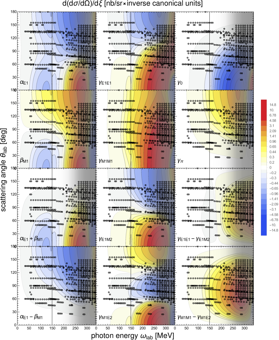
Figure 7: (Colour online) Sensitivity of the cross section to varying the polarisabilities, with a colour coding unique to this plot; see text for details.

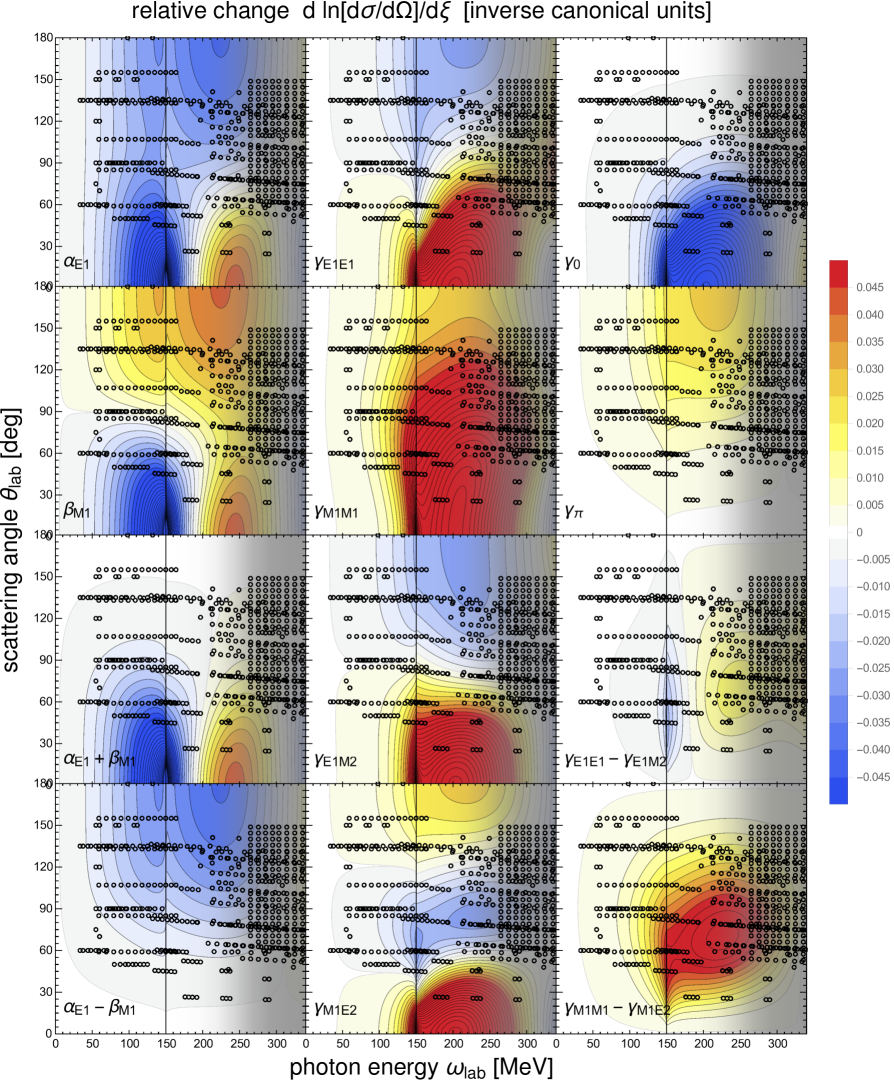
Figure 8: (Colour online) Sensitivity of the cross section to varying the polarisabilities, normalised to the cross section; see text for details.

3.6 Sensitivity of Asymmetries and Polarisation-Transfer Observables to Polarisabilities

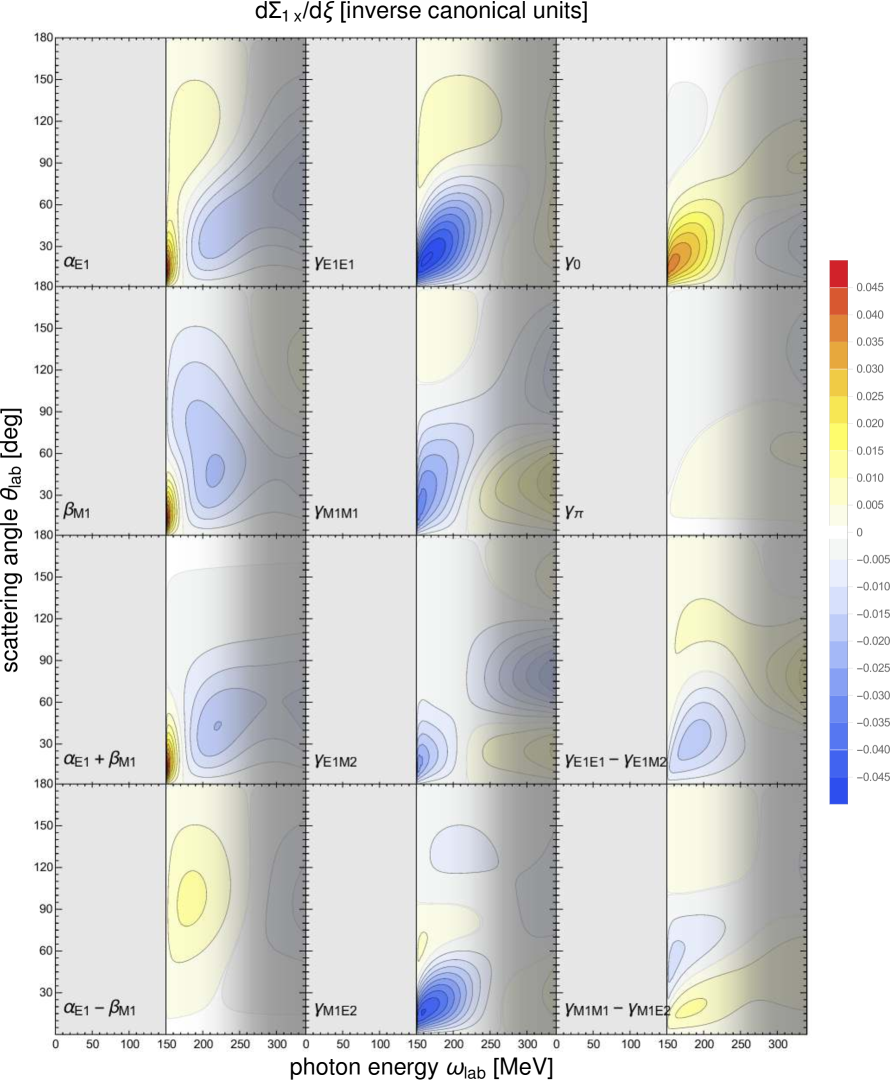
Figure 9: (Colour online) Sensitivity of the double asymmetry $\Sigma_{1x}$ (linearly polarised photons on a proton target polarised along the $x$ axis) to varying the polarisabilities; see text for details.

Figures 9 to 20 all use the same colour coding to indicate sensitivities to the polarisabilities as in fig. 8, now for the variation

$$\frac{\mathrm{d}\Sigma_{\alpha}}{\mathrm{d}\zeta}$$ (3.6)

of the asymmetry or polarisation-transfer observable $\Sigma_{\alpha}$ with respect to one of the polarisabilities $\zeta$. It varies between deep red ($\geq+0.045$ inverse canonical units) and deep blue ($\leq-0.045$), with additional contours when the extreme values of the colour scale are exceeded. All contours are separated by $0.005$ inverse canonical units.

The variations are in inverse units of $10^{-4}\;\mathrm{fm}^{3}$ for the scalar polarisabilities, and of $10^{-4}\;\mathrm{fm}^{4}$ for the spin ones. By a lucky coincidence, on these different scales the individual uncertainties are numerically roughly comparable (with all errors combined in quadrature): $\pm 0.9$ units for $\alpha_{E1}-\beta_{M1}$; $\pm 0.5$ for the individual scalar polarisabilities; and between $\pm 0.5$ and $\pm 0.8$ (different) units for the spin ones, with the exception of $\pm 1.9$ for $\gamma_{E1E1}$ [2]. Therefore, similar colours in the sensitivity plots also loosely correlate to similar impacts on improving the absolute size of polarisability values, even between scalar and spin polarisabilities, which are measured in different units.

It is important to reiterate the need for caution over the strong signals that exist for some variables around the Delta resonance. In this region, the theory is complete only at NLO, while the spin polarisabilities enter at a higher order than other neglected physics. The sensitivity that we see is genuine, but without an accurate description of the amplitudes, an extraction of the actual value of the polarisabilities should not be made.

We now list some observations. First, we consider the observables and make general comments on sensitivities, largely concentrating again on energies below 250 MeV, where the three essential conditions of sect. 3.4 are met. At this point, we are more concerned with the strength of signals than with their uniqueness, and indeed some of the most sensitive observables are affected by several of the polarisabilities. We will consider possible “sweet spots” that may allow the targetting of particular polarisabilities or combinations next. A cursory glance at the plots shows that there is almost no place with sensitivity to only one of the multipole-basis spin polarisabilities, whereas sensitivities to the combinations defined above are in general better separated. We will therefore confine our comments to those combinations.

• $\Sigma_{2x}$, $\Sigma_{2z}$, $\Sigma_{2x^{\prime}}$, and to a lesser extent $\Sigma_{2z^{\prime}}$ and $\Sigma_{3y}$, show the largest sensitivities. This is particularly notable, as it occurs not very far above the pion-production threshold. The sensitivity of $\Sigma_{3y^{\prime}}$, while sizeable, is largely at higher energies. For the other five, in most cases there is marked sensitivity to $\alpha_{E1}+\beta_{M1}$ and $\gamma_{0}$, and not exclusively at very forward angles. None has strong dependence on $\alpha_{E1}-\beta_{M1}$, but $\Sigma_{2z}$ is something of an exception, with at least some sensitivity even below threshold. $\gamma_{\pi}$ does not feature, either. The possible exceptions are again $\Sigma_{2z}$ and $\Sigma_{2z^{\prime}}$, which are also the only ones that do not vanish at backward angles. $\Sigma_{2x}$ and $\Sigma_{2x^{\prime}}$ display a strong dependence on $\gamma_{E-}$ around $\theta\approx 60^{\circ}$ and $\omega_{\mathrm{lab}}\approx 200\;\mathrm{MeV}$, and particularly for $\Sigma_{2x}$ this is paired with little sensitivity to $\alpha_{E1}-\beta_{M1}$ and the other spin polarisability combinations. $\Sigma_{2z}$ at mid angles and $\Sigma_{3y^{\prime}}$ at more forward angles have some sensitivity to $\gamma_{M-}$, and to some degree to $\gamma_{E-}$ as well. $\Sigma_{3y}$ has some very strong sensitivities at forward angles very close to threshold, but both its absolute magnitude and the cross section there are small.

  MAMI data, preliminary and published, exists for both $\Sigma_{2x}$, and $\Sigma_{2z}$ [15, 8, 18], all of which lies above the ideal energy region. Taking the sensitivity plots at face value, though, we see that the 288 MeV $\Sigma_{2x}$ data, though at a higher energy than peak sensitivity, is still sensitive primarily to $\gamma_{E-}$ and, to a lesser extent, to $\gamma_{\pi}$ and $\alpha_{E1}+\beta_{M1}$, with almost no sensitivity to the other combinations. The $\Sigma_{2z}$ data probes all the spin polarisabilities except $\gamma_{0}$, with little dependence on $\alpha_{E1}-\beta_{M1}$.

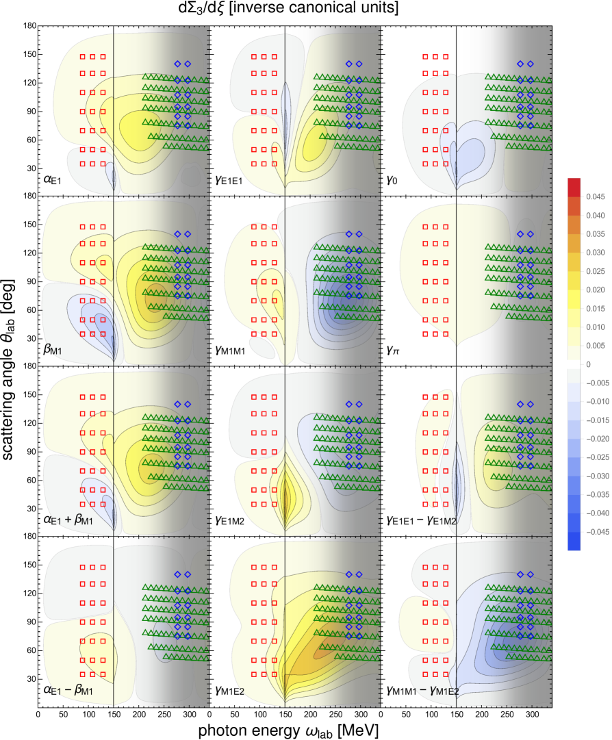
Figure 13: (Colour online) Sensitivity of the beam asymmetry $\Sigma_{3}$ (linearly polarised photons on an unpolarised proton target) to varying the polarisabilities; see text for details. Data symbols as in fig. 5.

• $\Sigma_{3}$: While the beam asymmetry has a reliably large magnitude below threshold, its sensitivity to the polarisabilities is limited there, see fig. 13. This is expected from the discussion in sect. 3.3, as the Thomson term provides a low-energy theorem for this observable. As noted in Ref. [45], at very low energy there is a linear dependence on $\beta_{M1}$, which however vanishes at $90^{\circ}$. It can easily be seen, though, that at most angles above 80 MeV, the dependence on $\alpha_{E1}$, though formally higher-order in the low-energy expansion, is actually as important as the one to $\beta_{M1}$, and that the sensitivity to $\alpha_{E1}-\beta_{M1}$ is particularly weak. Of the spin polarisabilities, though, only $\gamma_{0}$ has any influence below pion-threshold. This implies that below-pion-threshold, measurements of $\Sigma_{3}$, like those of ref. [9], or the $\Sigma_{3}$ data recently taken at HI$\gamma$S [38], will require high precision—and tight control of systematics—if they are to provide useful information on polarisabilities.

  Above 200 MeV, at mid angles, dependence on $\alpha_{E1}+\beta_{M1}$ and $\gamma_{M-}$ sets in, peaking around 250 MeV. There is no sensitivity to $\gamma_{\pi}$, almost none to $\alpha_{E1}-\beta_{M1}$, and even $\gamma_{0}$ has little effect in this region. If we exploit the Baldin sum rule, $\Sigma_{3}$ provides an opportunity to fix $\gamma_{M-}$ with only a little sensitivity to $\gamma_{E-}$.

• $\Sigma_{y}$: The region somewhat above the pion-production threshold and at moderate forward angles is sensitive to $\alpha_{E1}+\beta_{M1}$, with marked dependence on $\gamma_{0}$ and some on $\gamma_{M-}$ and $\gamma_{E-}$ developing at slightly higher energies. In view of the information already given by sum rules, this observable does not look very promising.

• $\Sigma_{1x}$ and, to a lesser extent, $\Sigma_{1x^{\prime}}$ show a strong pocket of sensitivity to $\gamma_{0}$ just above the pion-production threshold and at moderate forward angles. In $\Sigma_{1x^{\prime}}$, the sensitivity region is somewhat larger, shifted to less acute angles, and shows little dependence on the scalar polarisabilities. However, we also note that the cross section is quite small at forward angles around the pion threshold.

• $\Sigma_{1z}$ and $\Sigma_{1z^{\prime}}$: At moderate forward angles and at energies above 200 MeV, the polarisation transfer has increasing sensitivity to $\gamma_{E-}$ and $\gamma_{M-}$, with no contamination at all from $\alpha_{E1}-\beta_{M1}$ or $\gamma_{\pi}$. The best sensitivity, though, is at energies where results of different theoretical approaches may differ. Below 240 MeV, the asymmetry $\Sigma_{1z}$ has the smallest overall sensitivities of any observable. This would be a good place to test how well different theoretical approaches describe the non-structure part. Around $\theta\approx 60^{\circ}$ and $\omega_{\mathrm{lab}}\approx 200\;\mathrm{MeV}$, there is some mild sensitivity to $\gamma_{E-}$, with only a slight contamination from $\alpha_{E1}+\beta_{M1}$ and $\gamma_{0}$.

Turning this around, we now list, in no particular order, regions of marked sensitivity to various polarisability combinations, within the kinematic domain where we trust the theoretical extraction and cross sections are not exceedingly small. We are now particularly interested in isolated sensitivities, or at least those that become so when the forward sum rules are used to fix $\alpha_{E1}+\beta_{M1}$ and $\gamma_{0}$.

• $\gamma_{E-}$ in $\Sigma_{2x}$ for $30^{\circ}\lesssim\theta\lesssim 60^{\circ}$ and $200\leavevmode\nobreak\ {\rm MeV}\lesssim\omega_{\mathrm{lab}}\lesssim 250$ MeV. Though the sensitivity decreases with energy, it is still present in the region of some of the data of ref. [15, 8]. However, those data are at high enough energies that we begin to significantly mistrust theoretical extractions. In fact, our prediction is that the peak (absolute) sensitivity to $\gamma_{E-}$ in this observable is at lower energies and more forward angles than these data. At higher angles, $\gamma_{\pi}$ starts to play a role.

• $\gamma_{M-}$ in $\Sigma_{3}$ for $60^{\circ}\lesssim\theta\lesssim 90^{\circ}$ and $200\leavevmode\nobreak\ {\rm MeV}\lesssim\omega_{\mathrm{lab}}\lesssim 250\leavevmode\nobreak\ {\rm MeV}$, though sensitivity to $\gamma_{E-}$ is not absent. The LEGS data [39] overlaps this region, and re-examination of it in $\chi$EFT is likely worthwhile (cf. ref. [46, 20, 22]), especially in light of the preliminary MAMI results [16, 18] at kinematics which overlap the data of ref. [39]. $\theta\lesssim 60^{\circ}$ and energies of around 230 MeV in $\Sigma_{2z}$ are also promising for this polarisability.

• $\gamma_{E-}$ and $\gamma_{M-}$ affect almost every observable to some degree, and there is rarely contamination from $\alpha_{E1}-\beta_{M1}$ and $\gamma_{\pi}$ for angles less than $90^{\circ}$. For $\Sigma_{2x^{\prime}}$ and $\Sigma_{2z^{\prime}}$ and, to a lesser extent, for $\Sigma_{3y^{\prime}}$, $\Sigma_{3y}$ and $\Sigma_{1z^{\prime}}$, sensitivity to both combinations is present below 200 MeV. There is even a noticeable effect below pion-production threshold in $\Sigma_{2x^{\prime}}$. Strong dependence on both $\gamma_{E-}$ and $\gamma_{M-}$ is also found for $60^{\circ}\lesssim\theta\lesssim 90^{\circ}$ and energies around 230 MeV in $\Sigma_{2z}$. At lower energies, $\alpha_{E1}-\beta_{M1}$ is a confounding variable.

• $\gamma_{\pi}$ is hard to isolate. The vast majority of observables are almost completely insensitive to it below 240 MeV. Exceptions are $\Sigma_{2z}$ at around $150^{\circ}$ and 240 MeV, where fortunately sensitivity to $\alpha_{E1}-\beta_{M1}$ happens to be small, and $\Sigma_{2z^{\prime}}$ in a somewhat similar region. However, in the latter observable, sensitivity to $\alpha_{E1}-\beta_{M1}$ is not negligible.

• $\alpha_{E1}-\beta_{M1}$ is another combination with very limited opportunities for determinative measurements in asymmetries and polarisation-transfer observables. At central angles around the pion-production threshold, there is good sensitivity in $\Sigma_{2z}$ and $\Sigma_{2z^{\prime}}$, but not independent of $\gamma_{E-}$ and $\gamma_{M-}$.

• $\alpha_{E1}+\beta_{M1}$ affects many observables at forward angles, most notably $\Sigma_{2x^{\prime}}$ and $\Sigma_{2z}$, though usually in conjunction with $\gamma_{0}$. The strongest isolated sensitivity is well below threshold at moderate forward and backward angles in $\Sigma_{3}$ and $\Sigma_{2z^{\prime}}$, but it is hard to see experiments here reaching an accuracy that could rival the error bars of the Baldin sum rule.

• $\gamma_{0}$ dominates the sensitivities for a reasonable-sized region in $\Sigma_{1x^{\prime}}$: angles around $30^{\circ}$ and $\omega_{\mathrm{lab}}\approx 200$ MeV, and in $\Sigma_{y}$ in a rather narrower energy range at similar angles. Again, it is hard to see the sum rule being rigorously tested in any practical experiment here.

The bottom line is encouraging. If $\alpha_{E1}+\beta_{M1}$ and $\gamma_{0}$ are regarded as well-constrained by the forward sum rules, there are multiple opportunities to extract the spin-polarisability combinations $\gamma_{E-}$ and $\gamma_{M-}$ in regions that are experimentally accessible, theoretically clean and largely independent of the values of $\alpha_{E1}-\beta_{M1}$ and $\gamma_{\pi}$. Access to the scalar polarisabilities, to $\gamma_{0}$ and to $\gamma_{\pi}$ is best achieved through cross-section measurements, with coverage of markedly forward and backward angles being very useful in that regard.

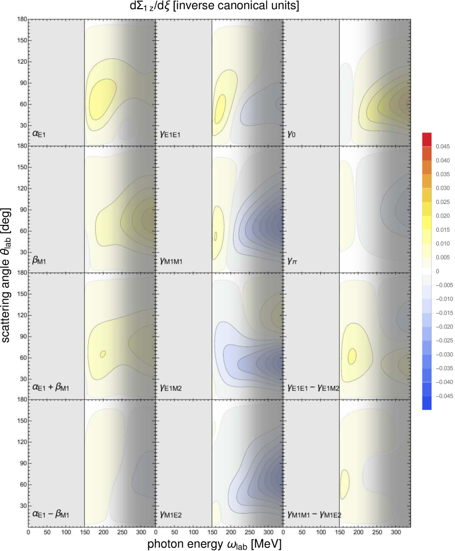
Figure 10: (Colour online) Sensitivity of the double asymmetry $\Sigma_{1z}$ (linearly polarised photons on a proton target polarised along the $z$ axis) to varying the polarisabilities; see text for details.

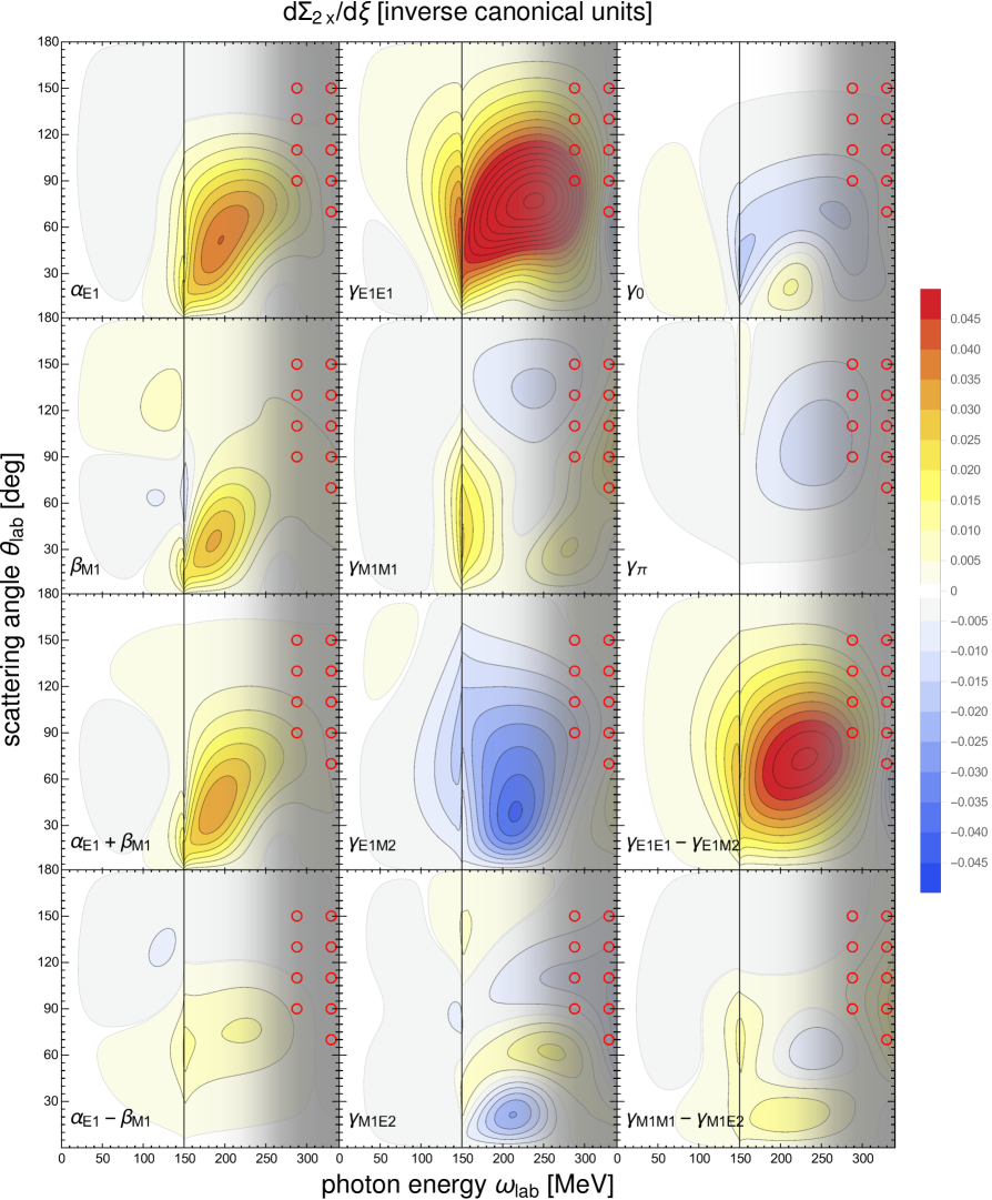
Figure 11: (Colour online) Sensitivity of the double asymmetry $\Sigma_{2x}$ (circularly polarised photons on a proton target polarised along the $x$ axis) to varying the polarisabilities; see text for details. Data symbols as in fig. 5; their size does not reflect the error bars, nor the size of energy or angle bins.

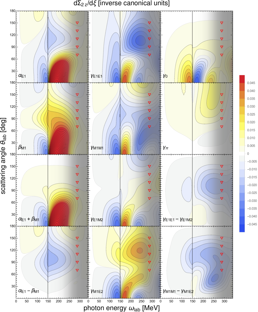
Figure 12: (Colour online) Sensitivity of the double asymmetry $\Sigma_{2z}$ (circularly polarised photons on a proton target polarised along the $z$ axis) to varying the polarisabilities; see text for details. Data symbols as in fig. 5; their size does not reflect the error bars, nor the size of energy or angle bins.

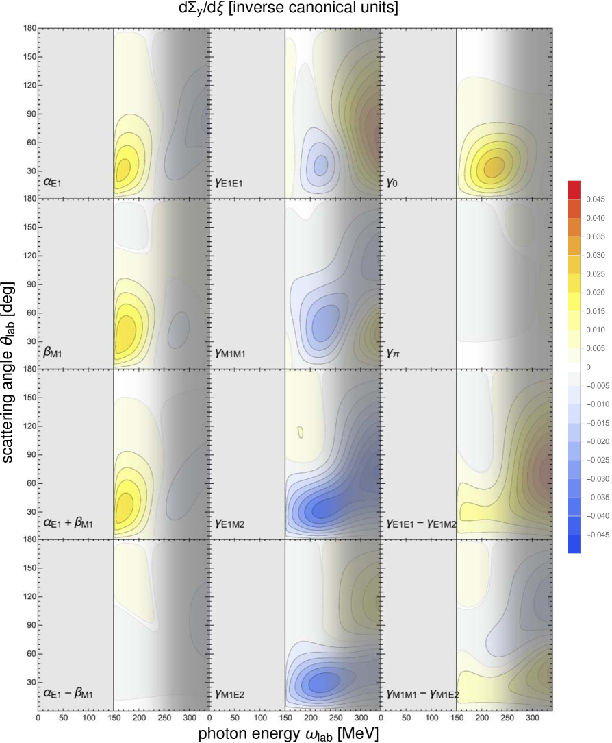
Figure 14: (Colour online) Sensitivity of the target asymmetry $\Sigma_{y}$ (unpolarised photons on a proton target along the $y$ axis) to varying the polarisabilities; see text for details.

Figure 15: (Colour online) Sensitivity of the double asymmetry $\Sigma_{3y}$ (linearly polarised photons on a proton target polarised along the $y$ axis) to varying the polarisabilities; see text for details.

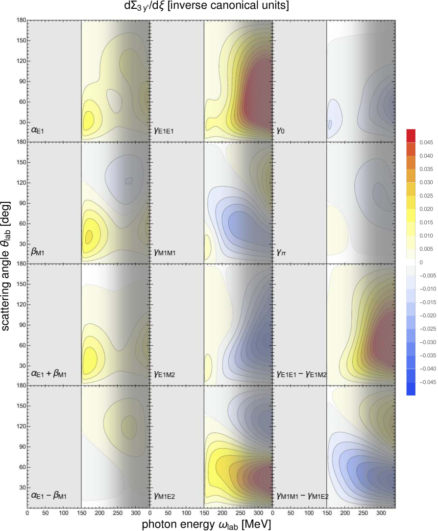
Figure 16: (Colour online) Sensitivity of the polarisation-transfer observable $\Sigma_{3y^{\prime}}$ (linearly polarised photons on an unpolarised proton target, recoil polarised along the $y^{\prime}$ axis) to varying the polarisabilities; see text for details.

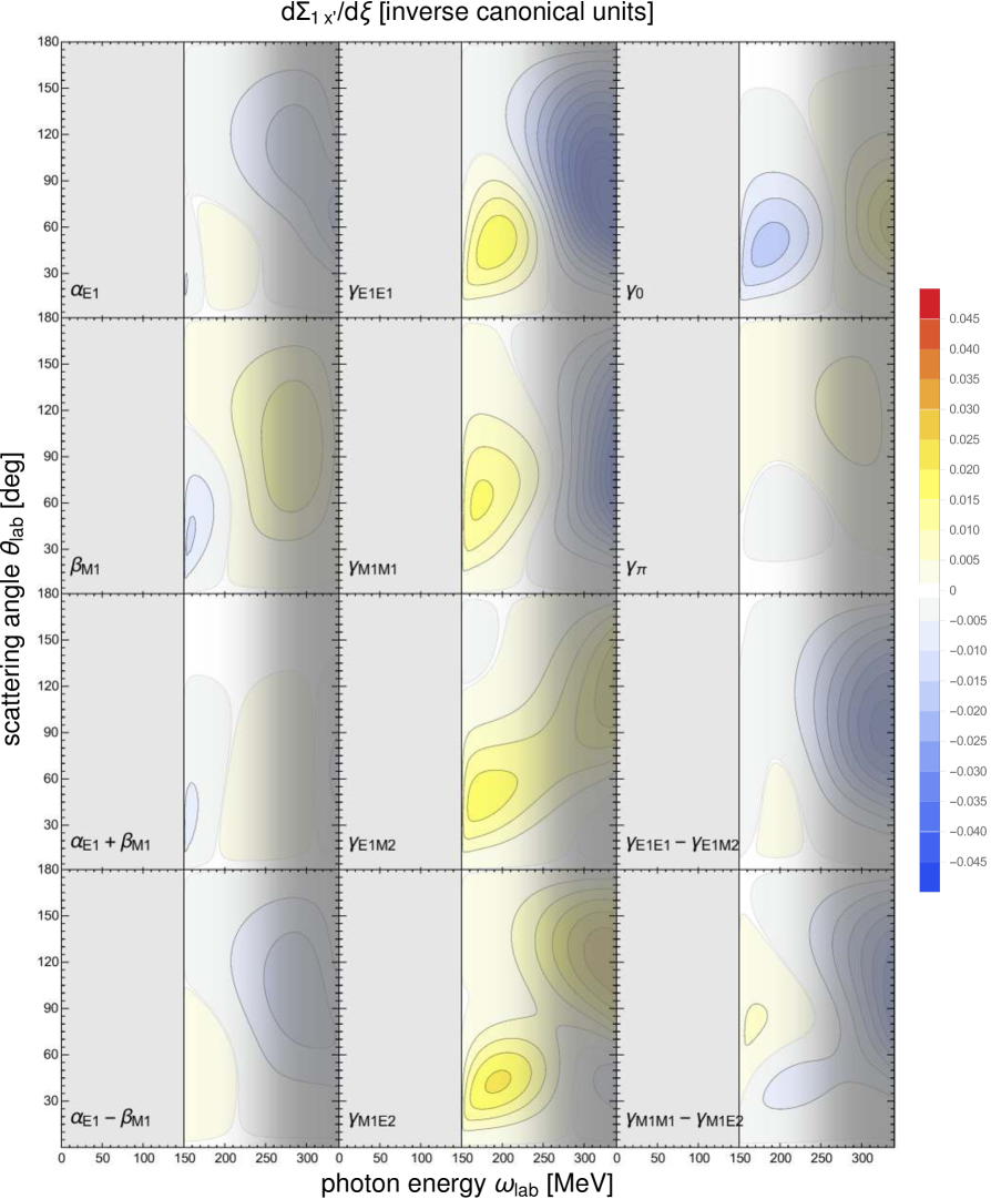
Figure 17: (Colour online) Sensitivity of the polarisation-transfer observable $\Sigma_{1x^{\prime}}$ (linearly polarised photons on an unpolarised proton target, recoil polarised along the $x^{\prime}$ axis) to varying the polarisabilities; see text for details.

Figure 18: (Colour online) Sensitivity of the polarisation-transfer observable $\Sigma_{1z^{\prime}}$ (linearly polarised photons to an unpolarised proton target, recoil polarised along the $z^{\prime}$ axis) to varying the polarisabilities; see text for details.

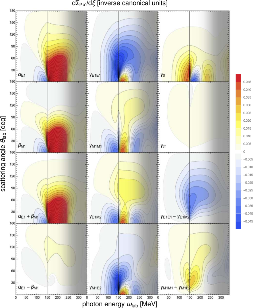
Figure 19: (Colour online) Sensitivity of the polarisation-transfer observable $\Sigma_{2x^{\prime}}$ (circularly polarised photons on an unpolarised proton target, recoil polarised along the $x^{\prime}$ axis) to varying the polarisabilities; see text for details.

Figure 20: (Colour online) Sensitivity of the polarisation-transfer observable $\Sigma_{2z^{\prime}}$ (circularly polarised photons to an unpolarised proton target, recoil polarised along the $z^{\prime}$ axis) to varying the polarisabilities; see text for details.

3.7 Neutron Observables

There are no free neutron targets stable and dense enough for meaningful Compton scattering experiments. But inelastic processes in quasi-free neutron kinematics can be approximated as free-neutron processes multiplied by the momentum distribution of the neutron inside a nucleus; see refs. [47, 48, 49] and references therein for descriptions of the unpolarised process on the deuteron. However, such an “Impulse Approximation” description is accurate only for energies well above the pion-production threshold. With these caveats in mind, in this section we present an overview of free-neutron Compton scattering observables in figs. 21 to 23. The atlas of sensitivities of observables to variations of the neutron polarisabilities is available in the online supplement (appendix D of the arXiv version), and also covered by the Mathematica notebook. For observables corresponding to $\Sigma_{2z}$, $\Sigma_{2x}$, $\Sigma_{2z}$, $\Sigma_{1x}$, $\Sigma_{1z}$ and $\Sigma_{3}$, results to order $e^{2}\delta^{3}$ for $\omega\lesssim 170\;\mathrm{MeV}$ were already presented in refs. [12, 13], and the effects of higher-multipole polarisabilities were again shown to be small. Here, we add one order, extend to higher energies, and provide a more comprehensive sensitivity study.

The neutron cross section is of course much smaller than the proton one at low energies due to the absence of the charged contributions to the Born amplitudes. Only pion-pole, magnetic-moment and structure effects are non-zero. Interestingly, it exceeds the proton cross section around the pion-production threshold, where charge-contributions are overwhelmed by the other Born and structure effects. Isospin symmetry guarantees that the two cross sections are very similar closer to the Delta resonance.

The sensitivity of all asymmetries and polarisation transfers to the spin polarisabilities is also much bigger than for the proton analogues. Quasielastic kinematics for $\omega_{\mathrm{lab}}\lesssim 250\;\mathrm{MeV}$ may therefore be an interesting venue to extract neutron spin polarisabilities: it is possible there are even better signals there than for the proton case.

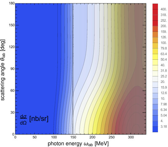
Figure 21: (Colour online) Contour plot of the unpolarised differential cross section for the neutron as a function of $\omega_{\mathrm{lab}}$ and $\theta$, on a logarithmic scale, and with additional contours for very small and very large values. The colour coding is identical to that of the corresponding fig. 4 for the proton.

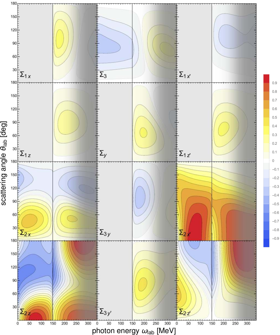
Figure 22: (Colour online) Contour plots of the asymmetries and polarisation-transfer observables for the neutron; see text for details.

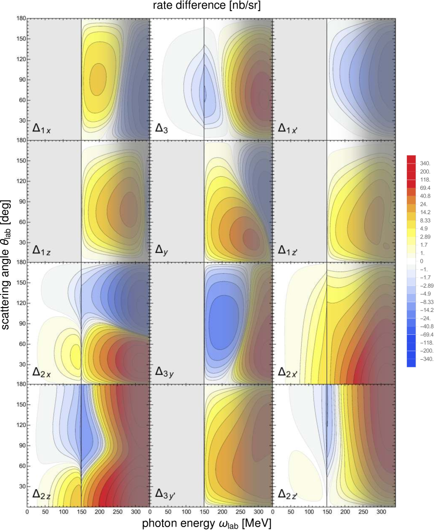
Figure 23: (Colour online) Contour plots of the rates associated with asymmetries and polarisation-transfer observables for the neutron, with additional contours for very small and very large values; see text for details. The colour coding is identical to that of the corresponding fig. 6 for the proton.

4 Summary and Conclusions

In this paper, we have provided a comprehensive study of asymmetries and polarisation-transfer observables for polarised photon scattering from a nucleon, including both polarised-target and recoil-polarisation-detection observables. Our main goal is to provide guidance to experimentalists planning the next generation of polarised Compton scattering experiments. We have used Chiral Effective Field Theory to calculate the magnitudes of the observables over the full range of angles and energies up to the peak of the $\Delta(1232)$ resonance. We have investigated the effects of varying the scalar and spin polarisabilities, with a view to identifying regions of particular sensitivity. The results presented here, supplemented by additional ones for the neutron, are also available as an interactive Mathematica notebook from judith.mcgovern@manchester.ac.uk.

We have also shown that, at a given energy and angle, the $6$ observables that do not vanish below the pion-production threshold suffice to determine the Compton amplitudes there. They form a “complete set of experiments” and in principle could be used to obtain the energy-dependence of the scalar and spin dipole polarisabilities from purely sub-threshold data—without the use of any sum-rule constraints. Above pion threshold, $5$ additional observables are needed if the Compton multipoles are to be completely determined from experiment. Polarisation-transfer observables are essential to such a programme. This is however not necessary to determine the static polarisabilities which were our focus.

The Baldin and forward-spin-polarisability sum rules constrain the polarisability combinations $\alpha_{E1}+\beta_{M1}$ and $\gamma_{0}$ quite tightly. While achieving concurrence with the sum-rule values is a worthy goal, it will be challenging for the experiments discussed here to improve upon them. Because of this, we placed particular emphasis on opportunities to pin down individual polarisabilities, as well as combinations such as $\alpha_{E1}-\beta_{M1}$, $\gamma_{E-}:=\gamma_{E1E1}-\gamma_{E1M2}$ and $\gamma_{M-}:=\gamma_{M1M1}-\gamma_{M1E2}$. This shows that a concerted effort to measure several asymmetries and polarisation transfers, in the various kinematics where we have identified sensitivities, is the optimum overall strategy. Definitive values of the spin polarisabilities will ultimately be established through the same procedure by which $\alpha_{E1}-\beta_{M1}$ has been determined: a comprehensive fit to a statistically consistent experimental database, with carefully formulated correlated and point-to-point systematic errors, that has been compiled at several labs around the world.

By comparing different approaches to calculating Compton amplitudes and by considering where the particular $\chi$EFT amplitude we used here is reliable, we have identified two distinct energy regions where such a campaign could be carried out with a minimum of theoretical bias.

In the low-energy region, i.e. below the pion-production threshold, we are confident in the $\chi$EFT predictions, with almost the only residual uncertainty being the precise value of the polarisabilities themselves. At these energies, plenty of high-quality cross section data is available, but there is only limited information on the asymmetries—only one is measured at all. Accurate experiments with good energy and angular range that explore the $6$ observables which do not vanish in this region are required to pin down all $6$ polarisabilities. However, though asymmetries can be large, the absolute rates are not huge and the sensitivities to the spin polarisabilities are quite modest in the main. Demands on beam time and control of systematics will certainly be high.

In the intermediate-energy region, namely between the pion threshold and $\omega_{\mathrm{lab}}\approx 250$ MeV, the agreement between $\chi$EFT and dispersion-relation calculations remains rather good, and both the cross section and sensitivities tend to rise rapidly. This is a region for which very limited data exist. It is therefore a promising avenue for further exploration. Once again, only one asymmetry has been explored, with limited coverage and accuracy. Indeed, significant gaps exist even in the $\gamma$p cross section data base. Measurements motivated by sensitivities to spin polarisabilities in this energy regime would thus likely have the added benefit of also delivering high-quality unpolarised data. This could help to resolve the disagreement between those proton Compton scattering experiments that accrued significant cross section data in this energy range (see Table 3.1 of ref. [24] and discussion in ref. [4]). Indeed, we argued that further information on $\alpha_{E1}$, $\beta_{M1}$, $\gamma_{0}$ and $\gamma_{\pi}$ will be most easily and reliably obtained from cross-section measurements—perhaps especially from cross-section measurements at markedly forward or backward angles.

At even higher energies, the cross sections and certain sensitivities become quite sizeable; however, the theoretical predictions of the underlying amplitudes in $\chi$EFT and the dispersion-relation approach start to diverge. Though high-statistics measurements in this region will challenge and discriminate between these two approaches, the comparisons may do little to shed light on the specific value of the polarisabilities. Accurate connection to the static polarisabilities, which are defined in the low-energy limit, is likely to be very challenging here.

Therefore, we propose that future explorations focus on a region in which three essential conditions are met: there are significant sensitivities to spin polarisabilities (usually $\omega_{\mathrm{lab}}\gtrsim 100\;\mathrm{MeV}$); theory can extract polarisabilities reliably and with high accuracy ($\omega_{\mathrm{lab}}\lesssim 250\;\mathrm{MeV}$); and experiments are not overwhelmed by backgrounds ($30^{\circ}\lesssim\theta\lesssim 160^{\circ}$). Within these constraints, we identified several kinematic regions where various asymmetries and polarisation-transfer observables are significantly affected by the spin-polarisability combinations $\gamma_{E-}$ and $\gamma_{M-}$, while being rather insensitive to $\alpha_{E1}-\beta_{M1}$ and $\gamma_{\pi}$.

We hope this presentation has provided indications of which proton Compton-scattering data are most promising for polarisability extractions. Nevertheless, complex sensitivities and the experimental challenges of small rates paired with polarised targets and/or recoils mean that no single experiment will suffice to determine a polarisability, or a simple combination thereof, in particular when it comes to the spin polarisabilities. Instead, what is needed is a comprehensive programme of mutually complementary experiments—ideally conducted at different facilities. As theorists, we recognise that there are many experimental realities that can prevent a promising observable or kinematic region from being the best place to do an experiment, and look forward to a lively exchange regarding the planning and analysis of the experiments at the new generation of experiments at high-luminosity facilities with polarised beams and targets such as HI$\gamma$S and MAMI.

Appendix A Dipole Polarisabilities of the Nucleon

For the convenience of the reader, we repeat in table 1 the values and uncertainties of the proton’s and neutron’s dipole scalar and spin polarisabilities obtained at $\mathcal{O}(e^{2}\delta^{4})$ in $\chi$EFT with explicit $\Delta(1232)$ degrees of freedom [4, 7, 2]. The theoretical uncertainties ($68\%$ degree-of-belief intervals) are derived from order-by-order convergence of the EFT. The scalar polarisabilities are determined from data [4, 7], with $\chi^{2}=113.2$ for $135$ degrees of freedom for the proton, and $45.2$ for $44$ for the neutron. The respective Baldin sum rules have been used as a constraint. (Note, though, that the extraction used $\alpha_{E1}^{(\mathrm{p})}+\beta_{M1}^{(\mathrm{p})}=13.8\pm 0.4$ [43]. This agrees within error bars with the more recent value $\alpha_{E1}^{(\mathrm{p})}+\beta_{M1}^{(\mathrm{p})}=14.0\pm 0.2$ [41].) The proton spin polarisability $\gamma_{M1M1}^{(\mathrm{p})}$ has been fitted as described in ref. [4], but $\gamma_{M1M1}^{(\mathrm{n})}$ is then predicted from that. Scalar polarisabilities are quoted in $10^{-4}\leavevmode\nobreak\ {\rm fm}^{3}$, spin ones in $10^{-4}\leavevmode\nobreak\ {\rm fm}^{4}$. A thorough discussion of all aspects can be found in ref. [2].

	proton	neutron
$\alpha_{E1}$	$10.65\pm 0.35_{\text{stat}}\pm 0.2_{\text{Baldin}}\pm 0.3_{\text{theory}}$	$11.55\pm 1.25_{\text{stat}}\pm 0.2_{\text{Baldin}}\pm 0.8_{\text{theory}}$
$\beta_{M1}$	$\phantom{0}3.15\mp 0.35_{\text{stat}}\pm 0.2_{\text{Baldin}}\mp 0.3_{\text{theory}}$	$\phantom{0}3.65\mp 1.25_{\text{stat}}\pm 0.2_{\text{Baldin}}\mp 0.8_{\text{theory}}$
$\gamma_{E1E1}$	$-1.1\pm 1.9_{\text{theory}}$	$-4.0\pm 1.9_{\text{theory}}$
$\gamma_{M1M1}$	$\phantom{-}2.2\pm 0.5_{\text{stat}}\pm 0.6_{\text{theory}}$	$\phantom{-}1.3\pm 0.5_{\text{stat}}\pm 0.6_{\text{theory}}$
$\gamma_{E1M2}$	$-0.4\pm 0.6_{\text{theory}}$	$-0.1\pm 0.6_{\text{theory}}$
$\gamma_{M1E2}$	$\phantom{-}1.9\pm 0.5_{\text{theory}}$	$\phantom{-}2.4\pm 0.5_{\text{theory}}$

Table 1: The dipole polarisabilities of the proton and neutron in $\chi$EFT with explicit $\Delta(1232)$ degrees of freedom at $\mathcal{O}(e^{2}\delta^{4})$ [4, 7, 2].

Appendix B Matrices for Observables

We provide here the definition of the Compton scattering amplitude in the Breit or cm frame and the relations between the $6$ independent amplitudes $A_{i}$ and the asymmetries and polarisation-transfer observables.

All the expressions required are given in Babusci et al. [11]. Those authors use a covariant basis to define $6$ independent amplitudes (which they denote simply $A_{i}$ but we will call $A_{i}^{\text{L}}$ as they are due to L’vov), and construct invariants $W^{\pm}_{ij}$ from these (the first index, $i=0,1,2,3$, refers to the photon polarisation, and the second, $j=0,1,2,3$, to the nucleon polarisation). Linear combinations of these invariants ($13$ of which are non-vanishing) give cross sections for polarised photons and nucleons (incoming or outgoing), and from these, in turn, asymmetries (absolute or relative) can be constructed.

In order to see the influence of the polarisabilities, though, it is more customary to use a basis of independent tensors constructed from Pauli matrices as follows:

$$\begin{array}[]{rcl}T(\omega,z)&=&A_{1}(\omega,z)\;(\vec{\epsilon}\,^{\prime*}\cdot\vec{\epsilon})+A_{2}(\omega,z)\;(\vec{\epsilon}\,^{\prime*}\cdot\hat{\vec{k}})\;(\vec{\epsilon}\cdot\hat{\vec{k}}^{\prime})\\ &&+\mathrm{i}\,A_{3}(\omega,z)\;\vec{\sigma}\cdot\left(\vec{\epsilon}\,^{\prime*}\times\vec{\epsilon}\,\right)+\mathrm{i}\,A_{4}(\omega,z)\;\vec{\sigma}\cdot\left(\hat{\vec{k}}^{\prime}\times\hat{\vec{k}}\right)(\vec{\epsilon}\,^{\prime*}\cdot\vec{\epsilon})\\ &&+\mathrm{i}\,A_{5}(\omega,z)\;\vec{\sigma}\cdot\left[\left(\vec{\epsilon}\,^{\prime*}\times\hat{\vec{k}}\right)\,(\vec{\epsilon}\cdot\hat{\vec{k}}^{\prime})-\left(\vec{\epsilon}\times\hat{\vec{k}}^{\prime}\right)\,(\vec{\epsilon}\,^{\prime*}\cdot\hat{\vec{k}})\right]\\ &&+\mathrm{i}\,A_{6}(\omega,z)\;\vec{\sigma}\cdot\left[\left(\vec{\epsilon}\,^{\prime*}\times\hat{\vec{k}}^{\prime}\right)\,(\vec{\epsilon}\cdot\hat{\vec{k}}^{\prime})-\left(\vec{\epsilon}\times\hat{\vec{k}}\right)\,(\vec{\epsilon}\,^{\prime*}\cdot\hat{\vec{k}})\right]\;\;.\end{array}$$ (B.1)

where $\hat{\vec{k}}$ ($\hat{\vec{k}}^{\prime}$) is the unit vector in the momentum direction of the incoming (outgoing) photon with polarisation $\vec{\epsilon}$ ($\vec{\epsilon}\,^{\prime*}$), $\theta$ is the scattering angle, and $z=\cos\theta$. This form holds in the Breit and centre-of-mass (cm) frames, and defines amplitudes $A_{i}^{\text{cm}}(\omega_{\text{cm}},z_{\text{cm}})$ or $A_{i}^{\text{Br}}(\omega_{\text{Br}},z_{\text{Br}})$.

The low-energy expansion of the non-Born parts of the Breit-frame amplitudes in terms of the polarisabilities, defined in eq. (2.1), is:

$$A_{1}^{\mathrm{Br}} =4\pi\left(\alpha_{E1}+z_{\text{Br}}\beta_{M1}\right)\omega_{\text{Br}}^{2}+{\cal O}(\omega_{\text{Br}}^{4})\;\;,$$

$$A_{2}^{\mathrm{Br}} =-4\pi\;\beta_{M1}\,\omega_{\text{Br}}^{2}+{\cal O}(\omega_{\text{Br}}^{4})\;\;,$$

$$A_{3}^{\mathrm{Br}} =-4\pi\left(\gamma_{E1E1}+\gamma_{E1M2}+z_{\text{Br}}(\gamma_{M1M1}+\gamma_{M1E2})\right)\omega_{\text{Br}}^{3}+{\cal O}(\omega_{\text{Br}}^{5})\;\;,$$

$$A_{4}^{\mathrm{Br}} =4\pi\left(\gamma_{M1E2}-\gamma_{M1M1}\right)\omega_{\text{Br}}^{3}+{\cal O}(\omega_{\text{Br}}^{5})\;\;,$$

$$A_{5}^{\mathrm{Br}} =4\pi\;\gamma_{M1M1}\,\omega_{\text{Br}}^{3}+{\cal O}(\omega_{\text{Br}}^{5})\;\;,$$

$$A_{6}^{\mathrm{Br}} =4\pi\;\gamma_{E1M2}\,\omega_{\text{Br}}^{3}+{\cal O}(\omega_{\text{Br}}^{5})\;\;.$$ (B.2)

The expression for the cm-frame amplitudes in terms of the cm photon energy and scattering angle is identical, except that the omitted terms all start at one order lower in $\omega$ because manifest crossing symmetry is lost. These new terms are all boost corrections and depend only on the same polarisabilities that already enter above.

When, in sects. 3.5 and 3.6, we vary the polarisabilities, we add to the chiral amplitudes terms mirroring eq. (B) with polarisability shifts $\delta\alpha_{E1}$, $\delta\beta_{M1}$, $\delta\gamma_{i}$ in place of full polarisabilities.

The relations between the covariant, cm and Breit amplitudes provided in ref. [22] allow the invariants that are expressed in terms of the $A_{i}^{\text{L}}$ in ref. [11] to be written in terms of the cm or Breit amplitudes. Writing the amplitudes as a vector, $\vec{A}=(A_{1},\dots,A_{6})^{T}$, invariants and observables are conveniently expressed as bilinears in $\vec{A}$: $\vec{A}^{\dagger}\,\mathcal{M}_{\alpha}\,\vec{A}$.

In the cm frame, these matrices $\mathcal{M}_{\alpha}$ for the observables $\mathcal{O}_{\alpha}$ all have a simple form and are independent of the photon energy, so we give those here. In what follows, $z=\cos\theta_{\text{cm}}$ and $A_{i}=A_{i}^{\text{cm}}$. As mentioned in sect. 2.1, the polarisabilities are most easily defined in the Breit frame, and that is the frame we use for our numerical work. However, the expressions for the matrices are the same in the $M_{\mathrm{N}}\to\infty$ limit, and the simpler forms in the cm frame allow one to see more clearly where the various amplitudes, and hence polarisabilities, play a role.

The unpolarised differential cross section is given by

$$\left.\frac{\mathrm{d}\sigma}{\mathrm{d}\Omega}\right|_{\text{unpol}}=\Phi^{2}\;|T|^{2}=\Phi^{2}\;\left(\vec{A}^{\dagger}\,\mathcal{M}_{\mathrm{d}\sigma}\,\vec{A}\right)$$ (B.3)

where $\Phi$ is the frame-dependent flux factor which tends to $1/4\pi$ at low energy (see, e.g., the review [24]). $|T|^{2}$ is calculated by averaging over the initial photon polarisation and nucleon spin, and summing over the final states. (It is what Babusci et al. call $W_{00}$, up to a normalisation factor of $4M_{\mathrm{N}}^{2}$.)

The matrix associated with $|T|^{2}$ is

$$\mathcal{M}_{\mathrm{d}\sigma}=\frac{1}{2}{\begin{pmatrix}z^{2}+1&z\left(z^{2}-1\right)&0&0&0&0\\ z\left(z^{2}-1\right)&\left(z^{2}-1\right)^{2}&0&0&0&0\\ 0&0&3-z^{2}&z-z^{3}&-2z\left(z^{2}-1\right)&4-4z^{2}\\ 0&0&z-z^{3}&1-z^{4}&-2z^{2}\left(z^{2}-1\right)&-2z\left(z^{2}-1\right)\\ 0&0&-2z\left(z^{2}-1\right)&-2z^{2}\left(z^{2}-1\right)&-4z^{4}+2z^{2}+2&-6z\left(z^{2}-1\right)\\ 0&0&4-4z^{2}&-2z\left(z^{2}-1\right)&-6z\left(z^{2}-1\right)&6-6z^{2}\end{pmatrix}}.$$ (B.4)

The asymmetries and polarisation-transfer observables $\Sigma_{\alpha}$ are then expressed by matrices $\mathcal{M}_{\alpha}$ which can also be derived from the customary relation between a cross section and the density matrices, see sect. 2.4: $\rho^{(\gamma)}(\vec{\xi})$ for the photon beam in terms of the Stokes parameters; $\rho(P,\vec{n})$ for the target; and $\rho(P^{\prime}\equiv 1,\vec{n}^{\prime})$ for the recoil. When the recoil polarisation is not detected, the cross section for a specific polarisation state is

$$\frac{\mathrm{d}\sigma}{\mathrm{d}\Omega}(P,\vec{n};\vec{\xi})=\Phi^{2}\;\mathrm{tr}[T\;\rho^{(\gamma)}(\vec{\xi})\;\rho(P,\vec{n})\;T^{\dagger}]\;\;.$$ (B.5)

For polarisation-transfer observables, one uses $\rho(P=0,\vec{n})=\frac{1}{2}$ for an unpolarised target:

$$\frac{\mathrm{d}\sigma}{\mathrm{d}\Omega}(\vec{n}^{\prime};\vec{\xi})=\frac{1}{2}\;\Phi^{2}\;\mathrm{tr}[T\;\rho^{(\gamma)}(\vec{\xi})\;T^{\dagger}\;\rho(P^{\prime}\equiv 1,\vec{n}^{\prime})]\;\;.$$ (B.6)

The matrix $\mathcal{M}_{\alpha}$ is then derived by inserting these relations into the definition of the corresponding observable $\Sigma_{\alpha}$ in eqs. (2.5) to (2.9) for the asymmetries and their analogue for the polarisation-transfer coefficients, with the normalisation such that

$$\Sigma_{\alpha}=\frac{\vec{A}^{\dagger}\,\mathcal{M}_{\alpha}\,\vec{A}}{2\;\vec{A}^{\dagger}\,\mathcal{M}_{\mathrm{d}\sigma}\,\vec{A}}\;\;.$$ (B.7)

A similar derivation yields the difference $\Delta_{\alpha}$ of the rates for the different orientations associated with each asymmetry or polarisation-transfer observable (see figs. 6 and  23 for plots). These are given by the numerator of eqs. (2.5) to (2.9) and the polarisation-transfer analogues, and are proportional to the numerator of (B.7),

$$\Delta_{\alpha}=\frac{g}{2}\;\Phi^{2}\;\vec{A}^{\dagger}\,\mathcal{M}_{\alpha}\,\vec{A}=g\;\Sigma_{\alpha}\;\left.\frac{\mathrm{d}\sigma}{\mathrm{d}\Omega}\right|_{\text{unpol}}\;\;,$$ (B.8)

with $g=4$ for $\Delta_{3y}$, $g=2$ for all other asymmetries and for $\Delta_{3y^{\prime}}$, and $g=1$ for the other polarisation-transfer observables. The denominator in the definition of each observable $\Sigma_{\alpha}$ (eqs. (2.5) to (2.9) and analogues) is $g\;\Phi^{2}\;\vec{A}^{\dagger}\,\mathcal{M}_{\mathrm{d}\sigma}\,\vec{A}$.

For the asymmetries, one finds:

$$\mathcal{M}_{3}=(1-z^{2}){\begin{pmatrix}-1&-z&0&0&0&0\\ -z&1-z^{2}&0&0&0&0\\ 0&0&1&z&2z&2\\ 0&0&z&z^{2}-1&2z^{2}&2z\\ 0&0&2z&2z^{2}&4z^{2}&4z\\ 0&0&2&2z&4z&4\end{pmatrix}}$$ (B.9)

$$\mathcal{M}_{y}=\mathrm{i}\sqrt{1-z^{2}}{\begin{pmatrix}0&0&-z&-z^{2}-1&-2z^{2}&-2z\\ 0&0&1-z^{2}&z-z^{3}&-2z\left(z^{2}-1\right)&2-2z^{2}\\ z&z^{2}-1&0&0&0&0\\ z^{2}+1&z\left(z^{2}-1\right)&0&0&0&0\\ 2z^{2}&2z\left(z^{2}-1\right)&0&0&0&0\\ 2z&2\left(z^{2}-1\right)&0&0&0&0\end{pmatrix}}$$ (B.10)

$$\mathcal{M}_{1x}=\mathrm{i}\sqrt{1-z^{2}}{\begin{pmatrix}0&0&z&0&z^{2}+1&2z\\ 0&0&z^{2}-1&0&z\left(z^{2}-1\right)&z^{2}-1\\ -z&1-z^{2}&0&z^{2}-1&z^{2}+1&2z\\ 0&0&1-z^{2}&0&z-z^{3}&1-z^{2}\\ -z^{2}-1&z-z^{3}&-z^{2}-1&z\left(z^{2}-1\right)&0&2\left(z^{2}-1\right)\\ -2z&1-z^{2}&-2z&z^{2}-1&2-2z^{2}&0\end{pmatrix}}$$ (B.11)

$$\mathcal{M}_{1z}=\mathrm{i}(1-z^{2}){\begin{pmatrix}0&0&-1&0&-z&-1\\ 0&0&-z&0&1-z^{2}&0\\ 1&z&0&-z&-z&-1\\ 0&0&z&0&z^{2}+1&2z\\ z&z^{2}-1&z&-z^{2}-1&0&0\\ 1&0&1&-2z&0&0\end{pmatrix}}$$ (B.12)

$$\mathcal{M}_{2x}=\sqrt{1-z^{2}}{\begin{pmatrix}0&0&-z&0&1-z^{2}&0\\ 0&0&1-z^{2}&0&z-z^{3}&1-z^{2}\\ -z&1-z^{2}&2z&z^{2}+1&3z^{2}-1&2z\\ 0&0&z^{2}+1&0&z\left(z^{2}-1\right)&1-z^{2}\\ 1-z^{2}&z-z^{3}&3z^{2}-1&z\left(z^{2}-1\right)&4z\left(z^{2}-1\right)&2\left(z^{2}-1\right)\\ 0&1-z^{2}&2z&1-z^{2}&2\left(z^{2}-1\right)&0\end{pmatrix}}$$ (B.13)

$$\mathcal{M}_{2z}={\begin{pmatrix}0&0&-z^{2}-1&0&z-z^{3}&z^{2}-1\\ 0&0&z-z^{3}&0&-\left(z^{2}-1\right)^{2}&0\\ -z^{2}-1&z-z^{3}&2\left(z^{2}-1\right)&z\left(z^{2}-1\right)&3z\left(z^{2}-1\right)&3\left(z^{2}-1\right)\\ 0&0&z\left(z^{2}-1\right)&0&\left(z^{2}-1\right)^{2}&0\\ z-z^{3}&-\left(z^{2}-1\right)^{2}&3z\left(z^{2}-1\right)&\left(z^{2}-1\right)^{2}&4z^{2}\left(z^{2}-1\right)&4z\left(z^{2}-1\right)\\ z^{2}-1&0&3\left(z^{2}-1\right)&0&4z\left(z^{2}-1\right)&4\left(z^{2}-1\right)\end{pmatrix}}$$ (B.14)

$$\mathcal{M}_{3y}=\mathrm{i}\sqrt{1-z^{2}}{\begin{pmatrix}0&0&-z&1-z^{2}&-2z^{2}&-2z\\ 0&0&1-z^{2}&z-z^{3}&-2z\left(z^{2}-1\right)&2-2z^{2}\\ z&z^{2}-1&0&0&-2&-2z\\ z^{2}-1&z\left(z^{2}-1\right)&0&0&0&0\\ 2z^{2}&2z\left(z^{2}-1\right)&2&0&0&2-2z^{2}\\ 2z&2\left(z^{2}-1\right)&2z&0&2\left(z^{2}-1\right)&0\end{pmatrix}}$$ (B.15)

And for the polarisation-transfer observables:

$$\mathcal{M}_{1x^{\prime}}=\mathrm{i}\sqrt{1-z^{2}}{\begin{pmatrix}0&0&-1&0&-2z&-z^{2}-1\\ 0&0&0&0&1-z^{2}&z-z^{3}\\ 1&0&0&0&2z&z^{2}+1\\ 0&0&0&0&z^{2}-1&z\left(z^{2}-1\right)\\ 2z&z^{2}-1&-2z&1-z^{2}&0&2z\left(z^{2}-1\right)\\ z^{2}+1&z\left(z^{2}-1\right)&-z^{2}-1&z-z^{3}&-2z\left(z^{2}-1\right)&0\end{pmatrix}}$$ (B.16)

$$\mathcal{M}_{1z^{\prime}}=\mathrm{i}(1-z^{2}){\begin{pmatrix}0&0&0&0&-1&-z\\ 0&0&1&0&0&1-z^{2}\\ 0&-1&0&-1&1&z\\ 0&0&1&0&2z&z^{2}+1\\ 1&0&-1&-2z&0&2\left(z^{2}-1\right)\\ z&z^{2}-1&-z&-z^{2}-1&2-2z^{2}&0\end{pmatrix}}$$ (B.17)

$$\mathcal{M}_{2x^{\prime}}=\sqrt{1-z^{2}}{\begin{pmatrix}0&0&-1&0&0&z^{2}-1\\ 0&0&0&0&z^{2}-1&z\left(z^{2}-1\right)\\ -1&0&2&2z&2z&3-z^{2}\\ 0&0&2z&0&z^{2}-1&z-z^{3}\\ 0&z^{2}-1&2z&z^{2}-1&0&-2z\left(z^{2}-1\right)\\ z^{2}-1&z\left(z^{2}-1\right)&3-z^{2}&z-z^{3}&-2z\left(z^{2}-1\right)&4-4z^{2}\end{pmatrix}}$$ (B.18)

$$\mathcal{M}_{2z^{\prime}}={\begin{pmatrix}0&0&2z&0&z^{2}-1&z-z^{3}\\ 0&0&z^{2}-1&0&0&-\left(z^{2}-1\right)^{2}\\ 2z&z^{2}-1&0&1-z^{2}&z^{2}-1&z\left(z^{2}-1\right)\\ 0&0&1-z^{2}&0&0&\left(z^{2}-1\right)^{2}\\ z^{2}-1&0&z^{2}-1&0&4z\left(z^{2}-1\right)&2\left(z^{4}-1\right)\\ z-z^{3}&-\left(z^{2}-1\right)^{2}&z\left(z^{2}-1\right)&\left(z^{2}-1\right)^{2}&2\left(z^{4}-1\right)&4z\left(z^{2}-1\right)\end{pmatrix}}$$ (B.19)

$$\mathcal{M}_{3y^{\prime}}=\mathrm{i}\sqrt{1-z^{2}}{\begin{pmatrix}0&0&-z&1-z^{2}&-2z^{2}&-2z\\ 0&0&1-z^{2}&z-z^{3}&-2z\left(z^{2}-1\right)&2-2z^{2}\\ z&z^{2}-1&0&0&2&2z\\ z^{2}-1&z\left(z^{2}-1\right)&0&0&0&0\\ 2z^{2}&2z\left(z^{2}-1\right)&-2&0&0&2\left(z^{2}-1\right)\\ 2z&2\left(z^{2}-1\right)&-2z&0&2-2z^{2}&0\end{pmatrix}}$$ (B.20)

The matrices are either real or imaginary, but are, of course, always Hermitean. The matrices for $\Sigma_{y}$, $\Sigma_{1x}$, $\Sigma_{1z}$, $\Sigma_{3y}$, $\Sigma_{1x^{\prime}}$, $\Sigma_{1z^{\prime}}$ and $\Sigma_{3y^{\prime}}$ are pure imaginary but the observables are real because the observables are nonzero only when the amplitudes have imaginary parts, i.e. above the first inelasticity, namely in our case above the pion-production threshold.

It is, of course, possible to take linear combinations of amplitudes to form a new set, each of which depends on a single polarisability or polarisability combination. The corresponding “rotation” matrices can be used to transform the matrices above, in order to see whether particular combinations of amplitudes dominate in either basis. The most noticeable result is that both $\Delta_{3}$ and $\Delta_{y}$ turn out to be completely independent of both $\gamma_{0}$ and $\gamma_{\pi}$—in the cm frame. This is particularly significant for $\Delta_{3}$, since it raises the possibility that for energies around the photoproduction threshold, once $\alpha_{E1}$ and $\beta_{M1}$ are well-determined, sensitivity to $\gamma_{E-}$ and $\gamma_{M-}$ is not contaminated by lack of knowledge of $\gamma_{\pi}$. For higher energies, the boost corrections which arise in the lab frame reduce the significance of these observations, see below.

In fact, all matrices except $\mathcal{M}_{{\mathrm{d}\sigma}}$, $\mathcal{M}_{3y}$ and $\mathcal{M}_{3y^{\prime}}$ have two zero eigenvalues, which means that there are two linear combinations of amplitudes to which they are insensitive. However, other than in the cases of $\mathcal{M}_{3}$ and $\mathcal{M}_{y}$, the corresponding eigenvectors do not indicate simple combinations of polarisabilities. Even more interesting results emerge if we look at combinations of double polarisation observables $\mathcal{M}_{ij}\pm\mathcal{M}_{ij^{\prime}}$. $\mathcal{M}_{3y}+\mathcal{M}_{3y^{\prime}}$ has two zero eigenvalues, and all other combinations of this form have four, and so are sensitive to only two combinations of amplitudes. However, only some of these zero modes correspond to simple combinations of amplitudes. This analysis does reveal, though, that the sum of $\mathcal{M}_{3y}$ and $\mathcal{M}_{3y^{\prime}}$ is insensitive to $\gamma_{0}$ and $\gamma_{\pi}$, while the difference is insensitive to $\alpha_{E1}$ and $\beta_{M1}$. The combinations $\mathcal{M}_{1x}-\mathcal{M}_{1x^{\prime}}$ and $\mathcal{M}_{1z}+\mathcal{M}_{1z^{\prime}}$ are completely insensitive to both $\alpha-\beta$ and $\gamma_{0}$, while the opposite combinations are insensitive to $\alpha+\beta$ and $\gamma_{\pi}$. Sums and differences of $\mathcal{M}_{2x}$ and $\mathcal{M}_{2x^{\prime}}$, or of $\mathcal{M}_{2z}$ and $\mathcal{M}_{2z^{\prime}}$, pair the insensitivities up the opposite way round.

Though this is an intriguing observation, the asymmetry and polarisation-transfer reactions are sufficiently different that it may not be significant for experimental design. And experiments are not conducted in the cm frame, in which the above decomposition holds, but in the lab frame; this complicates matters. That complication is least important for observables which transform easily between frames.

The incident photon and target nucleon polarisations are identical in all frames which share the same orientations of the $x$, $y$ and $z$ axes; this includes the Breit, cm, and lab frames. Therefore, all asymmetries are form-invariant, i.e. to find the lab results, one only has to convert the scattering angle and photon energy from the cm to the lab frame:

$$\Sigma_{\alpha}^{\mathrm{lab}}(\omega_{\mathrm{lab}},\theta_{\mathrm{lab}})=\Sigma_{\alpha}^{\mathrm{cm}}(\omega_{\mathrm{cm}}[\omega_{\mathrm{lab}},\theta_{\mathrm{lab}}],\theta_{\mathrm{cm}}[\omega_{\mathrm{lab}},\theta_{\mathrm{lab}}])\;\mbox{ for }j\not\in\{x^{\prime},z^{\prime}\}$$ (B.21)

The situation is slightly more complicated for polarisation-transfer coefficients, as the polarisation of the outgoing nucleon is measured relative to its momentum vector, i.e. the $z^{\prime}$ axis is oriented along $\vec{p}^{\,\prime}$, and the $x^{\prime}$ axis is perpendicular to it but in the scattering plane. In this case, the appropriate coefficients are different for cm and lab frames, and are given for both in ref. [11]. They are simply related by a rotation in the reaction plane through $\theta_{R}$, the angle in the lab frame from the $z$- to the $z^{\prime}$-axis, see fig. 2. In order to conserve momentum perpendicular to the incoming photon direction, they must satisfy

$$\sin\theta_{R}=\frac{\omega^{\prime}_{\mathrm{lab}}\sin\theta}{|\vec{p}^{\prime}|},\qquad 0\leq\theta_{R}\leq\pi/2,$$ (B.22)

where $\omega^{\prime}_{\mathrm{lab}}$ is the outgoing photon energy. Then, for $i=1,2$,

$$\Sigma_{ix^{\prime}}^{\mathrm{lab}} =\cos\theta_{R}\Sigma_{ix^{\prime}}^{\mathrm{cm}}-\sin\theta_{R}\Sigma_{iz^{\prime}}^{\mathrm{cm}},$$

$$\Sigma_{iz^{\prime}}^{\mathrm{lab}} =\sin\theta_{R}\Sigma_{ix^{\prime}}^{\mathrm{cm}}+\cos\theta_{R}\Sigma_{iz^{\prime}}^{\mathrm{cm}}.$$ (B.23)

On the other hand, the orientation of the $y$ axis is unchanged, and so the polarisation transfer $\Sigma_{3y^{\prime}}$ is form-invariant and obeys an equation like (B.21).

Appendix C Comments on Babusci et al.

C.1 Interpreting Coefficients

For the dedicated student of the invaluable paper of Babusci et al. [11], in an aside which is not intended to be read independently, we note that the lab-frame coefficients defined there as rather ugly expressions in their eq. (3.29) can also be written more intuitively as

$$\begin{split}C_{x^{\prime}}^{K}&=-{\textstyle\frac{1}{2}}\left[\omega_{\mathrm{lab}}\sin(\theta_{R})+\omega^{\prime}_{\mathrm{lab}}\sin(\theta+\theta_{R})\right]\\ C_{z^{\prime}}^{K}&={\textstyle\frac{1}{2}}\left[\omega_{\mathrm{lab}}\cos(\theta_{R})+\omega^{\prime}_{\mathrm{lab}}\cos(\theta+\theta_{R}]\right)\\ C_{z^{\prime}}^{Q}&={\textstyle\frac{1}{2}}\left[\omega_{\mathrm{lab}}\cos(\theta_{R})-\omega^{\prime}_{\mathrm{lab}}\cos(\theta+\theta_{R})\right]\;\;.\end{split}$$ (C.1)

It may seem odd that, up to signs, these are just the $x^{\prime}$ and $z^{\prime}$ coefficients of the lab-frame vectors $\vec{K}$ and $\vec{Q}$ (defined as ${\textstyle\frac{1}{2}}(\vec{k}^{\prime}\pm\vec{k})$), even though the struck nucleon is not at rest in that frame. The explanation is that a boost into its rest frame just exchanges $\vec{k}$ and $\vec{k}^{\prime}$ and changes the sign of the $z^{\prime}$ components, so that $\vec{K}$ and $\vec{Q}$ are trivially related in the rest frames of the target and recoiling nucleons.

C.2 Proving Completeness

Babusci et al. [11] provide a complete set of observables in which at most one nucleon and one photon are polarised or analysed, and, at the beginning of their sect. III.B, they hint that the amplitudes can be reconstructed from them. We now use the definition of observables in terms of the quadratic forms with matrices $\mathcal{M}_{\alpha}$ in appendix B to provide an explicit proof of this, following the presentation in Arenhövel et al. [50].

We start with the $6$ observables $\mathrm{d}\sigma/\mathrm{d}\Omega$, $\Sigma_{3}$, $\Sigma_{2x/z}$ and $\Sigma_{2x^{\prime}/z^{\prime}}$ which are nonzero below the first inelasticity (pion-production threshold). We denote these observables $\mathcal{O}_{\alpha\mathbb{R}}$, with $\alpha\mathbb{R}=1,\dots,6$. They are related to the real, independent amplitudes $A_{1\text{-}6}$ as before,

$$\mathcal{O}_{\alpha\mathbb{R}}\propto\vec{A}^{\dagger}\;\mathcal{M}_{\alpha\mathbb{R}}\;\vec{A}\;\;,$$ (C.2)

where the six $6\times 6$ matrices $\mathcal{M}_{\alpha\mathbb{R}}$ are real as well. The constants of proportionality are irrelevant for the present purpose.

To show that at fixed $(\omega,\theta)$, the amplitudes $\vec{A}$ can be constructed from $6$ observables $\mathcal{O}_{\alpha\mathbb{R}}$, one follows Arenhövel et al. [50] to combine (any) one column from each of the $\mathcal{M}_{\alpha\mathbb{R}}$ into a new $6\times 6$ matrix $H_{\mathbb{R}}^{\text{col}}$. Here, the superscript reminds us that there are $6^{6}$ choices possible. If at least one of these has a nonzero determinant,

$$\det H_{\mathbb{R}}^{\text{col}}\neq 0\;\;\mbox{ for some choice of columns,}$$ (C.3)

then the column vectors residing in that $H_{\mathbb{R}}^{\text{col}}$ are linearly independent and span the $6$-dimensional space in which the scalar product eq. (C.2) lives. The vector $\vec{A}$ can be reconstructed, and therefore the observables $\mathcal{O}_{\alpha\mathbb{R}}$ form a complete set of observables. Taking column $1$ from $\mathrm{d}\sigma/\mathrm{d}\Omega$, $\Sigma_{3}$, $\Sigma_{2x}$ and $\Sigma_{2x^{\prime}}$, and column $3$ from $\Sigma_{2z}$ and $\Sigma_{2z^{\prime}}$ produces one of many $H_{\mathbb{R}}^{\text{col}}$ of non-zero determinant, and so shows that these $6$ observables suffice to reconstruct the $6$ amplitudes below the pion-production threshold. Possible (discrete) sign ambiguities can be removed by requiring that amplitudes evolve continuously in $\omega$ and $\theta$ from the Thomson limit.

We now apply this method to the situation above the first inelasticity. There, the amplitudes are complex, $\vec{A}=\mathrm{Re}\vec{A}+\mathrm{i}\,\mathrm{Im}\vec{A}$, and the matrices $\mathcal{M}_{\alpha\mathbb{I}}$ ($\alpha\mathbb{I}=7,\dots,13$) of the $7$ additional observables are all purely imaginary. Therefore, the scalar product in eq. (C.2) takes on two different forms for the two types of observables (Einstein’s Summation Convention is understood):

$$\mathcal{O}_{\alpha\mathbb{R}}=(\mathrm{Re}[A_{i}]\mathrm{Re}[A_{j}]+\mathrm{Im}[A_{i}]\mathrm{Im}[A_{j}])\;\mathcal{M}_{\alpha\mathbb{R}}^{ij}\;\;\mbox{ and }\;\;\mathcal{O}_{\alpha\mathbb{I}}=-2\mathrm{i}\,\;\mathrm{Re}[A_{i}]\mathrm{Im}[A_{j}]\,\mathcal{M}_{\alpha\mathbb{I}}^{ij}$$ (C.4)

We turn this quadratic form into a scalar product between real vectors by defining a $12$-dimensional vector space via $\vec{u}^{T}=(\mathrm{Re}[\vec{A}]^{T},\mathrm{Im}[\vec{A}]^{T})$ in which the observables are found from real and symmetric $12\times 12$ matrices

$$\begin{pmatrix}\mathcal{M}_{\alpha\mathbb{R}}&0\\ 0&\mathcal{M}_{\alpha\mathbb{R}}\end{pmatrix}\;\;\mbox{ and }\;\;\begin{pmatrix}0&(-\mathrm{i}\mathcal{M}_{\alpha\mathbb{I}})^{T}\\ -\mathrm{i}\mathcal{M}_{\alpha\mathbb{I}}&0\end{pmatrix}\;\;.$$ (C.5)

However, one can only determine $11$ real parameters of the amplitudes, with the overall phase free. Therefore, one may without loss of generality choose one imaginary part $y_{j_{0}}$, $j_{0}\in\{7,\dots,12\}$, and eliminate it from the vector space by deleting the $j_{0}$th row of the vector $\vec{u}$. We denote the resulting $11$-dimensional vector by $\vec{u}^{\bcancel{j}_{0}}$. The matrices then turn into $11\times 11$ objects

$$\begin{pmatrix}\mathcal{M}_{\alpha\mathbb{R}}&0\\ 0&\mathcal{M}_{\alpha\mathbb{R}}^{\bcancel{j}_{0}\bcancel{j}_{0}}\end{pmatrix}\;\;\mbox{ and }\;\;\begin{pmatrix}0&(-\mathrm{i}\mathcal{M}_{\alpha\mathbb{I}}^{\bcancel{j}_{0}})^{T}\\ -\mathrm{i}\mathcal{M}_{\alpha\mathbb{I}}^{\bcancel{j}_{0}}&0\end{pmatrix}\;\;,$$ (C.6)

where the superscripts indicate that the lower $\mathcal{M}_{\alpha\mathbb{R}}$ block has become a $5\times 5$ matrix by elimination of the $j_{0}$th row and column, and $\mathcal{M}_{\alpha\mathbb{I}}$ an object with $6$ columns and $5$ rows by elimination of its $j_{0}$th row.

We now construct matrices analogous to $H_{\mathbb{R}}^{\text{col}}$. First, pick any $11$ of the available $13$ observables, then assemble one column of each into an $11\times 11$ matrix $H_{\mathbb{C}}^{\text{col}}$. If

$$\det H_{\mathbb{C}}^{\text{col}}\neq 0\;\;\mbox{ for some choice of columns,}$$ (C.7)

then this set of observables suffices to determine $\vec{u}^{\bcancel{j}_{0}}$ and hence the amplitudes $A_{1\text{-}6}$, up to the overall phase. This method described by Arenhövel et al. [50] for complex quadratic forms is more general, but we will now take advantage of the fact that our matrices $\mathcal{M}_{\alpha}$ are either real or imaginary.

Our search simplifies if we start by choosing the $6$ observables which were already used to find $\vec{A}$ below threshold. In this way, we exploit the block-diagonal structure of the matrices in Eq. (C.6), by writing

$$H_{\mathbb{C}}^{\text{col}}=\begin{pmatrix}A&0\\ 0&B\end{pmatrix}\;\;.$$ (C.8)

and choosing $A=H_{\mathbb{R}}^{\text{col}}$. We then only need to augment these $6$ observables by $5$ linearly-independent columns from the set of matrices of the additional above-threshold observables, ${\cal M}_{\alpha\mathbb{I}}$, which will then make up the matrix $B=H_{\mathbb{I}}^{\text{col}}$, and finally show that

$$\det H_{\mathbb{I}}^{\text{col}}\neq 0\;\;\mbox{ for some choice of columns.}$$ (C.9)

This can be done by picking one column apiece from any $5$ of the $7$ new observables, with any one row $(\bcancel{j}_{0}-6)$ eliminated. For example, one can construct $B$ by dropping $\Sigma_{3y}$ and $\Sigma_{3y^{\prime}}$, combining column $1$ of $\Sigma_{y}$, $\Sigma_{1x}$ and $\Sigma_{1x^{\prime}}$ with column $3$ of $\Sigma_{1z}$ and $\Sigma_{1z^{\prime}}$, and eliminating the $1$st row.

Therefore, this set of observables suffices to determine the amplitudes $A_{i}$ up to discrete ambiguities and an overall phase. This is not the most general set of observables above threshold, since we used the fact that the observables $\mathcal{O}_{\alpha\mathbb{R}}$ already can be turned into matrices $H_{\mathbb{R}}^{\text{col}}$ with nonzero determinants, but it suffices.

It should be mentioned that the imaginary parts of the amplitudes may also be reconstructed as multipoles of the total photoproduction cross sections [21]. This may provide alternative input or valuable cross checks, in particular in order to reduce error bars or sign ambiguities. The sign ambiguity $\vec{A}\to-\vec{A}$ and the overall phase may be resolvable by requiring that amplitudes evolve continuously in $\omega$ and $\theta$ from low-energy theorems (like the Thomson limit), whose phases are determined by choice.

Finally, our proof resorted to the observables expressed in terms of the matrices $\mathcal{M}_{\alpha}$ in the cm frame. The Lorentz boost into the lab frame only involves kinematic factors and cannot generate new linear or quadratic dependencies. Unsurprisingly then, the lab frame Compton amplitudes for spin-$\frac{1}{2}$ targets can also be reconstructed from the $6$ observables $\mathrm{d}\sigma/\mathrm{d}\Omega$, $\Sigma_{3}$, $\Sigma_{2x/z}$ and $\Sigma_{2x^{\prime}/z^{\prime}}$, supplemented above the pion-production threshold with any $5$ of the $7$ observables $\Sigma_{y}$, $\Sigma_{1x/z}$, $\Sigma_{1x^{\prime}/z^{\prime}}$, $\Sigma_{3y}$ and $\Sigma_{3y^{\prime}}$. To do a “complete experiment” below the first inelasticity, it is therefore mandatory to perform at least two polarisation transfer experiments, and at least one more is necessary above threshold.

Appendix D Online Supplement: Sensitivity of Neutron Observables

For ease of comparison, each plot uses the same contour map as the corresponding proton plot. The values of the neutron polarisabilities, including theoretical and experimental uncertainties, are summarised in ref. [2] and appendix A.

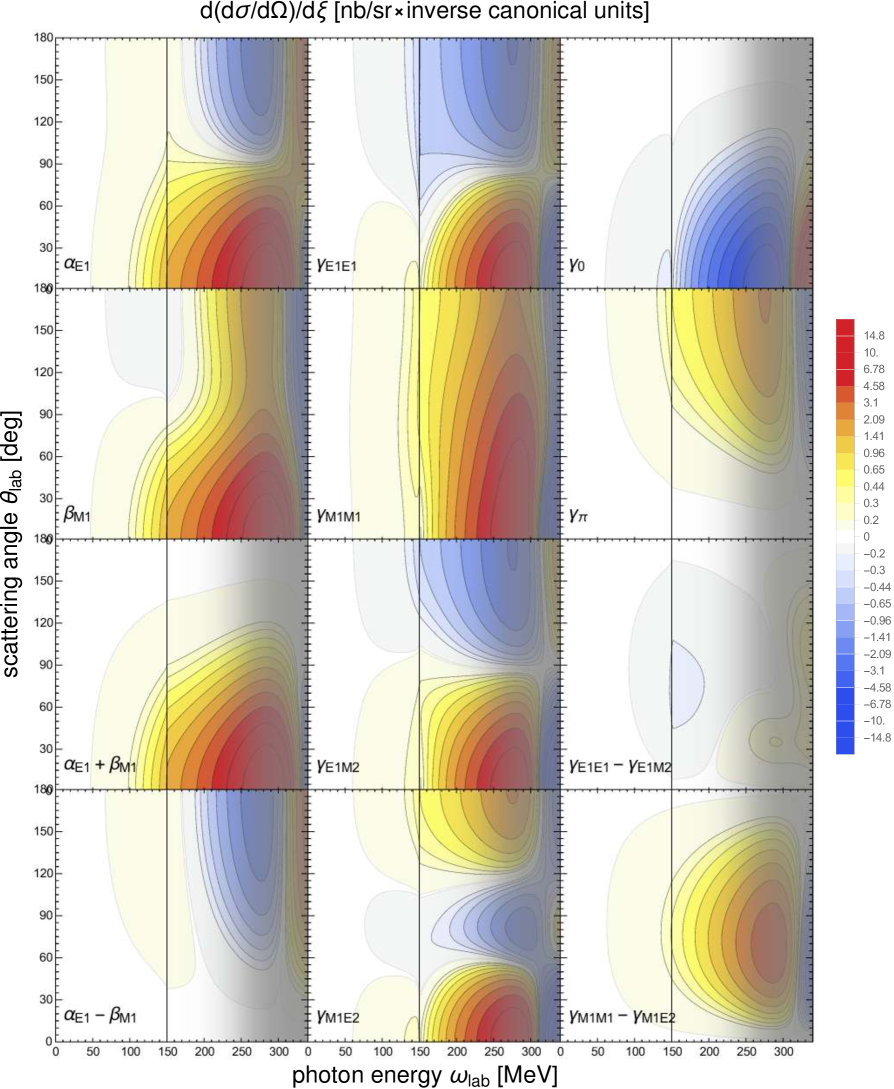
Figure 24: (Colour online) Sensitivity of the neutron cross section to varying the polarisabilities.

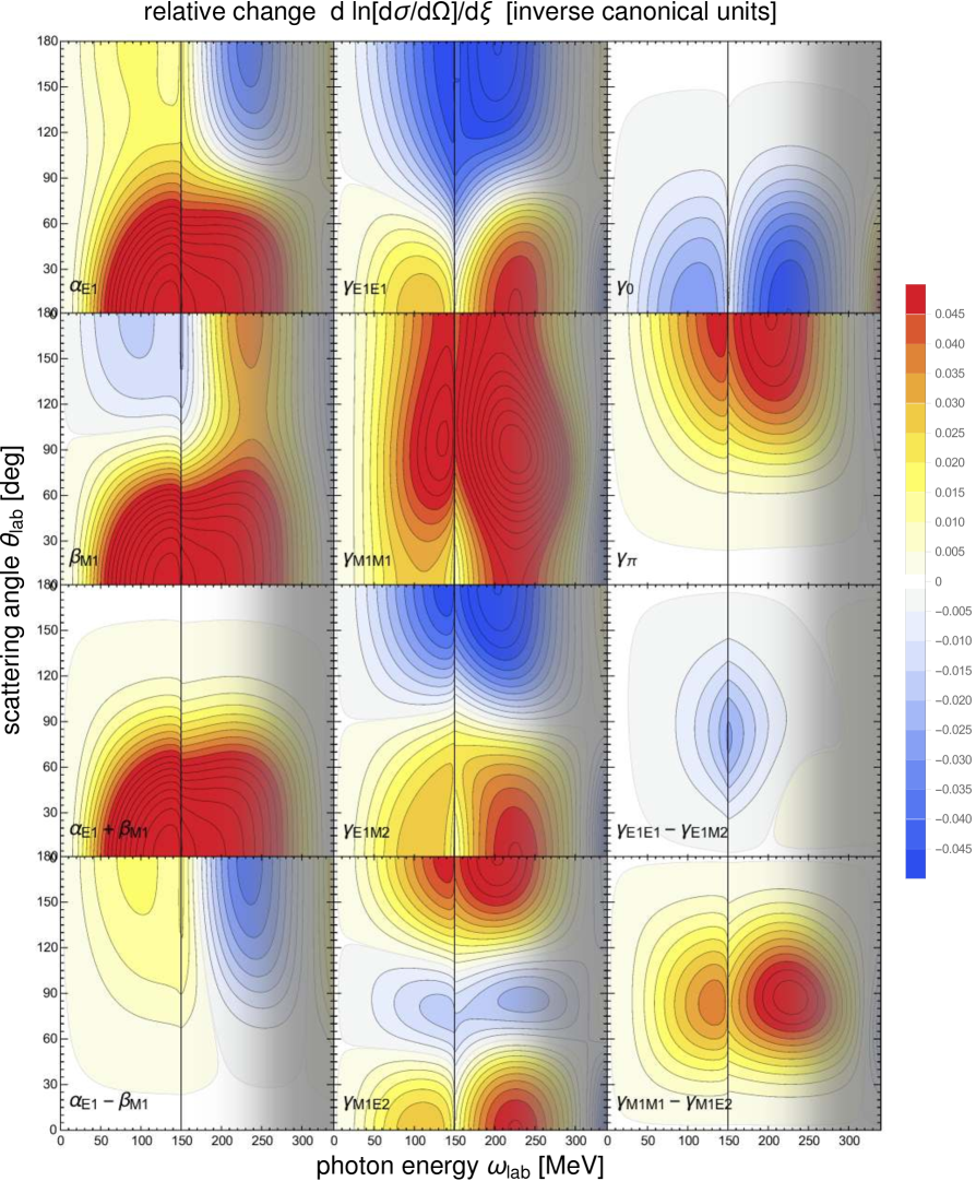
Figure 25: (Colour online) Sensitivity of the neutron cross section to varying the polarisabilities, normalised to the cross section.

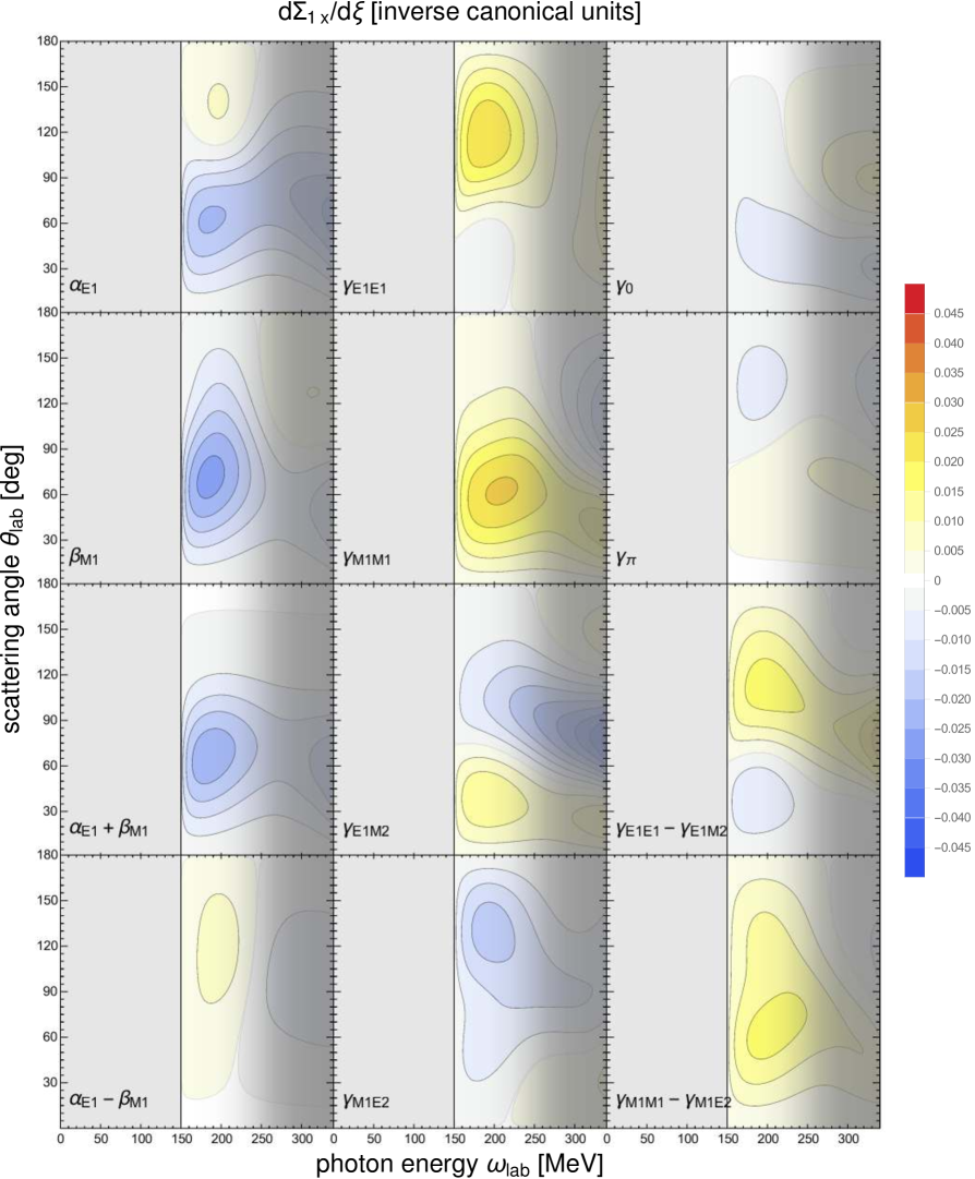
Figure 26: (Colour online) Sensitivity of the double asymmetry $\Sigma_{1x}$ (linearly polarised photons on a neutron target polarised along the $x$ axis) to varying the polarisabilities.

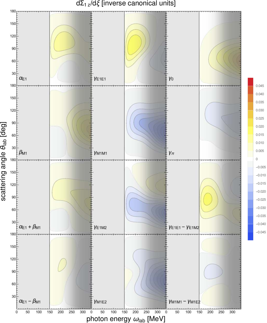
Figure 27: (Colour online) Sensitivity of the double asymmetry $\Sigma_{1z}$ (linearly polarised photons on a neutron target polarised along the $z$ axis) to varying the polarisabilities.

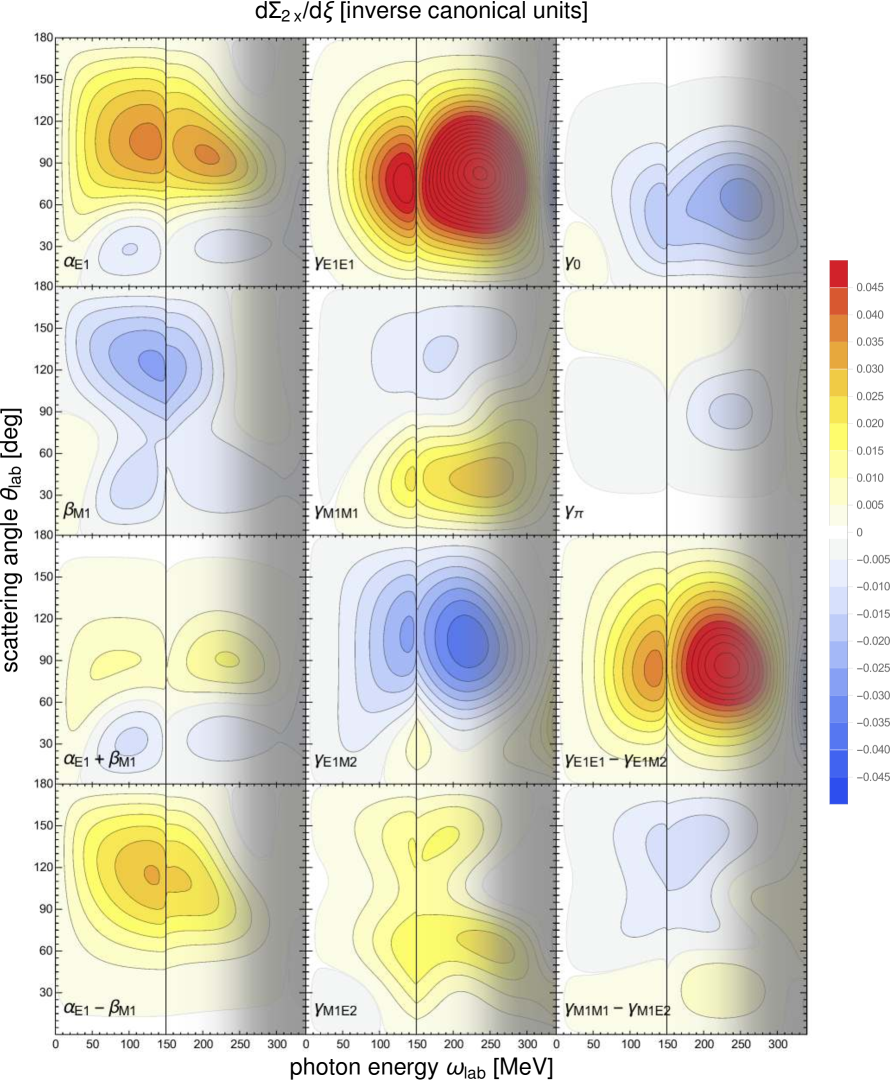
Figure 28: (Colour online) Sensitivity of the double asymmetry $\Sigma_{2x}$ (circularly polarised photons on a neutron target polarised along the $x$ axis) to varying the polarisabilities; see text for details.

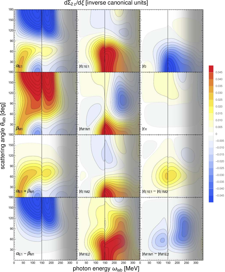
Figure 29: (Colour online) Sensitivity of the double asymmetry $\Sigma_{2z}$ (circularly polarised photons on a neutron target polarised along the $z$ axis) to varying the polarisabilities.

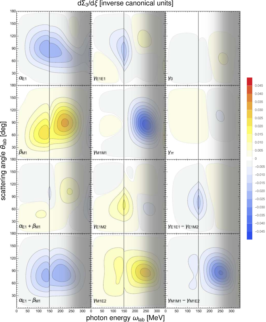
Figure 30: (Colour online) Sensitivity of the beam asymmetry $\Sigma_{3}$ (linearly polarised photons on an unpolarised neutron target) to varying the polarisabilities.

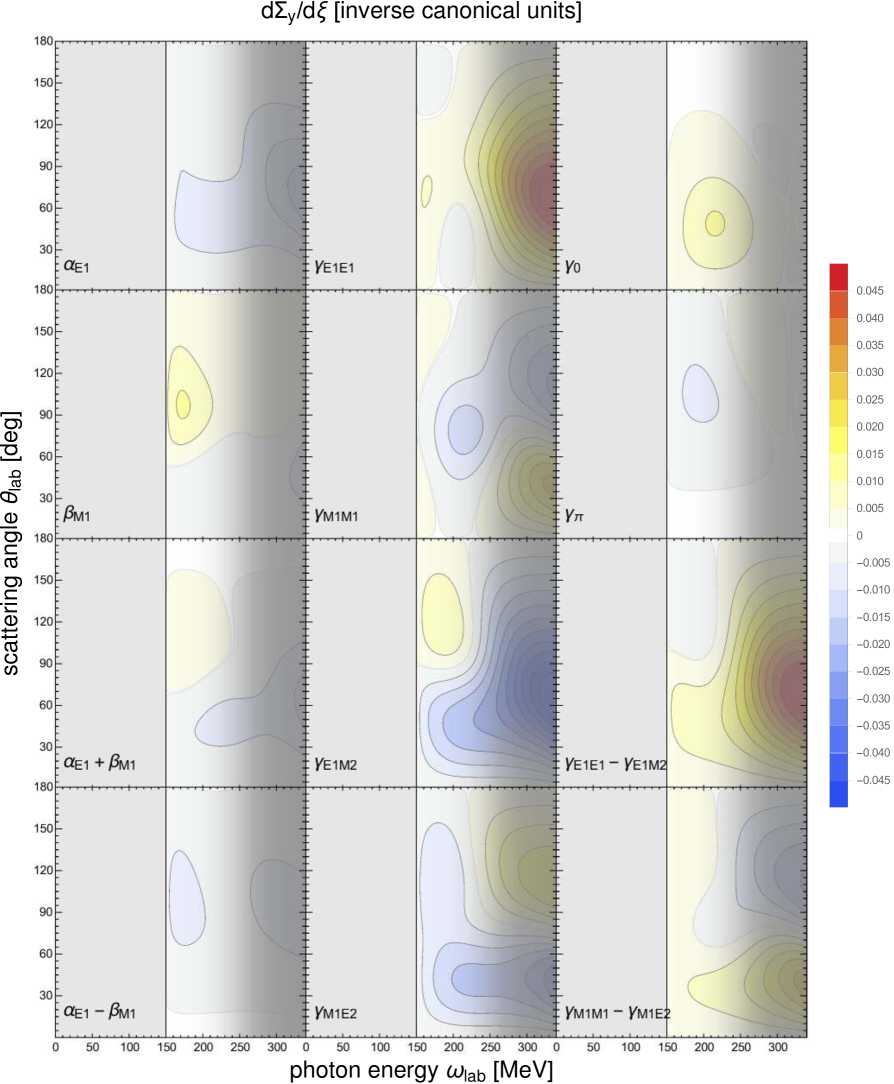
Figure 31: (Colour online) Sensitivity of the target asymmetry $\Sigma_{y}$ (unpolarised photons on a neutron target along the $y$ axis) to varying the polarisabilities.

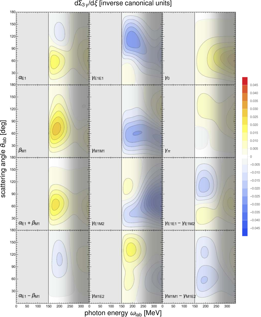
Figure 32: (Colour online) Sensitivity of the double asymmetry $\Sigma_{3y}$ (linearly polarised photons on a neutron target polarised along the $y$ axis) to varying the polarisabilities.

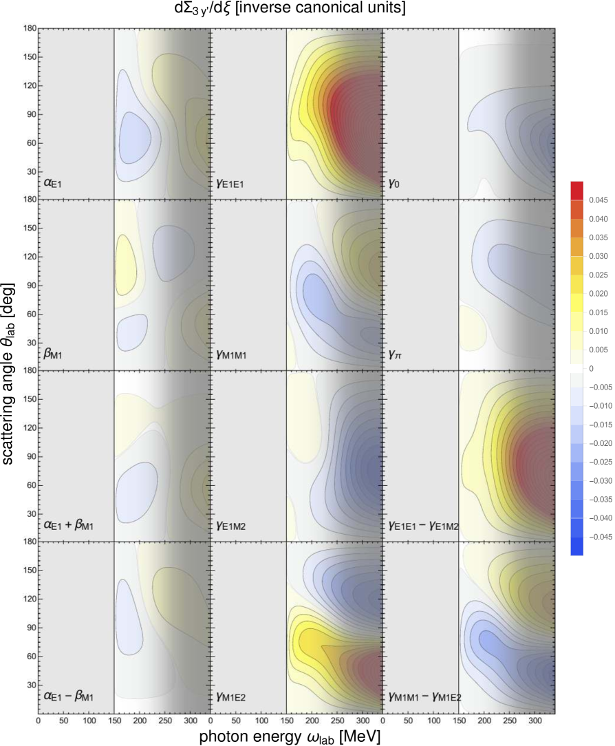
Figure 33: (Colour online) Sensitivity of the polarisation-transfer observable $\Sigma_{3y^{\prime}}$ (linearly polarised photons on an unpolarised neutron target, recoil polarised along the $y^{\prime}$ axis) to varying the polarisabilities.

Figure 34: (Colour online) Sensitivity of the polarisation-transfer observable $\Sigma_{1x^{\prime}}$ (linearly polarised photons on an unpolarised neutron target, recoil polarised along the $x^{\prime}$ axis) to varying the polarisabilities.

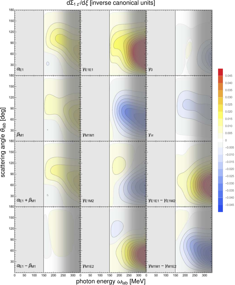
Figure 35: (Colour online) Sensitivity of the polarisation-transfer observable $\Sigma_{1z^{\prime}}$ (linearly polarised photons on an unpolarised neutron target, recoil polarised along the $z^{\prime}$ axis) to varying the polarisabilities.

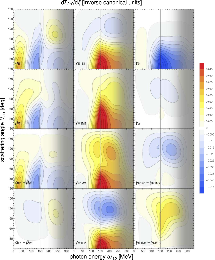
Figure 36: (Colour online) Sensitivity of the polarisation-transfer observable $\Sigma_{2x^{\prime}}$ (circularly polarised photons on an unpolarised neutron target, recoil polarised along the $x^{\prime}$ axis) to varying the polarisabilities.

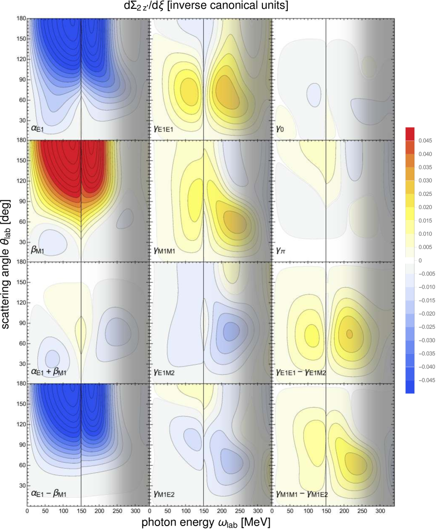
Figure 37: (Colour online) Sensitivity of the polarisation-transfer observable $\Sigma_{2z^{\prime}}$ (circularly polarised photons on an unpolarised neutron target, recoil polarised along the $z^{\prime}$ axis) to varying the polarisabilities.

References

- [1] R. E. Prange, Phys. Rev. 110 (1958) 240.
- [2] H. W. Grießhammer, J. A. McGovern and D. R. Phillips, Eur. Phys. J. A 52, no. 5 (2016) 139 [arXiv:1511.01952 [nucl-th]].
- [3] D. Drechsel, B. Pasquini and M. Vanderhaeghen, Phys. Rept. 378 (2003) 99 [arXiv:hep-ph/0212124].
- [4] J. A. McGovern, D. R. Phillips and H. W. Grießhammer, Eur. Phys. J. A 49 (2013) 12 [arXiv:1210.4104 [nucl-th]].
- [5] V. Lensky and J. A. McGovern, Phys. Rev. C 89 (2014) 032202 [arXiv:1401.3320 [nucl-th]].
- [6] B. Pasquini, P. Pedroni and S. Sconfietti, [arXiv:1711.07401 [hep-ph]].
- [7] L. S. Myers et al. [COMPTON@MAX-lab Collaboration], Phys. Rev. Lett. 113 (2014) no.26, 262506 [arXiv:1409.3705 [nucl-ex]].
- [8] P. P. Martel et al. [A2 Collaboration], Phys. Rev. Lett. 114 (2015) 112501 [arXiv:1408.1576 [nucl-ex]].
- [9] V. Sokhoyan et al. [A2 Collaboration], Eur. Phys. J. A 53, no. 1 (2017) 14 [arXiv:1611.03769 [nucl-ex]].
- [10] H. W. Grießhammer, A. I. L’vov, J. A. McGovern, V. Pascalutsa, B. Pasquini and D. R. Phillips, [arXiv:1409.1512 [nucl-th]].
- [11] D. Babusci, G. Giordano, A. I. L’vov, G. Matone and A. M. Nathan, Phys. Rev. C 58 (1998) 1013 [hep-ph/9803347] .
- [12] R. P. Hildebrandt, H. W. Grießhammer and T. R. Hemmert, Eur. Phys. J. A 20 (2004) 329 [arXiv:nucl-th/0308054].
- [13] R. P. Hildebrandt, PhD thesis, Technische Universität München (2005) [nucl-th/0512064].
- [14] B. Pasquini, D. Drechsel and M. Vanderhaeghen, Phys. Rev. C 76 (2007) 015203 [arXiv:0705.0282 [hep-ph]].
- [15] P. Martel, PhD Thesis, University of Massachusetts, Amherst (2012) https://wwwa2.kph.uni-mainz.de/images/publications/phd/pmartel_dis.pdf
- [16] C. Collicott, PhD Thesis, Dalhousie University (2015) https://wwwa2.kph.uni-mainz.de/images/publications/phd/thesis_Collicott-Cristina-2015.pdf
- [17] G. M. Huber and C. Collicott, [arXiv:1508.07919 [nucl-ex]].
- [18] P. Martel et al. [A2 Collaboration], EPJ Web Conf. 142 (2017) 01021.
- [19] H. W. Grießhammer, J. A. McGovern and D. R. Phillips, AIP Conf. Proc. 1735 (2016) 040010 [arXiv:1509.09177 [nucl-th]].
- [20] J. McGovern, H. Grießhammer and D. Phillips, PoS CD 15 (2015) 024.
- [21] R. P. Hildebrandt, H. W. Grießhammer, T. R. Hemmert and B. Pasquini, Eur. Phys. J. A 20 (2004) 293 [nucl-th/0307070].
- [22] V. Lensky, J. McGovern and V. Pascalutsa, Eur. Phys. J. C 75 (2015) no.12, 604 [arXiv:1510.02794 [hep-ph]].
- [23] B. R. Holstein, D. Drechsel, B. Pasquini and M. Vanderhaeghen, Phys. Rev. C 61 (2000) 034316 [hep-ph/9910427].
- [24] H. W. Grießhammer, J. A. McGovern, D. R. Phillips and G. Feldman, Prog. Part. Nucl. Phys. 67 (2012) 841 [arXiv:1203.6834 [nucl-th]]
- [25] V. Pascalutsa and D. R. Phillips, Phys. Rev. C 67 (2003) 055202 [nucl-th/0212024].
- [26] C. Patrignani et al. [Particle Data Group], Chin. Phys. C 40, no.10 (2016) 100001.
- [27] V. Pascalutsa, M. Vanderhaeghen and S. N. Yang, Phys. Rept. 437 (2007) 125 [hep-ph/0609004].
- [28] L. W. Cawthorne and J. A. McGovern, PoS CD 15 (2016) 072 [arXiv:1510.09136 [nucl-th]].
- [29] H. W. Grießhammer and T. R. Hemmert, Phys. Rev. C 65 (2002) 045207 [nucl-th/0110006].
- [30] H. W. Griesshammer, Prog. Part. Nucl. Phys. 55 (2005) 215 [nucl-th/0411080].
- [31] N. Krupina, V. Lensky and V. Pascalutsa, [arXiv:1712.05349 [nucl-th]].
- [32] V. Lensky and V. Pascalutsa, Eur. Phys. J. C 65, 195 (2010) [arXiv:0907.0451 [hep-ph]].
- [33] B. Pasquini, private communication.
- [34] B. Strandberg, A. Margaryan, H. W. Grießhammer, J. A. McGovern, D. R. Phillips and D. Shukla, in preparation.
- [35] H. W. Grießhammer, Eur. Phys. J. A 49 (2013) 100; Erratum: [Eur. Phys. J. A 53 (2017) no.5, 113] [arXiv:1304.6594 [nucl-th]].
- [36] G. G. Ohlsen, Rept. Prog. Phys. 35 (1972) 717.
- [37] M. H. Sikora et al., Phys. Rev. Lett. 112, no. 2 (2014) 022501 [arXiv:1309.7897 [nucl-ex]].
- [38] M. Ahmed, private communication (2017).
- [39] G. Blanpied, M. Blecher, A. Caracappa, R. Deininger, C. Djalali, G. Giordano, K. Hicks and S. Hoblit et al., Phys. Rev. C 64 (2001) 025203.
- [40] J.D. Jackson, Classical Electrodynamics, Wiley, 1998.
- [41] O. Gryniuk, F. Hagelstein and V. Pascalutsa, Phys. Rev. D 92 (2015) 074031 [arXiv:1508.07952 [nucl-th]].
- [42] O. Gryniuk, F. Hagelstein and V. Pascalutsa, Phys. Rev. D 94, no. 3 (2016) 034043 [arXiv:1604.00789 [nucl-th]].
- [43] V. Olmos de Leon et al., Eur. Phys. J. A 10 (2001) 207.
- [44] B. Pasquini, P. Pedroni and D. Drechsel, Phys. Lett. B 687 (2010) 160 [arXiv:1001.4230 [hep-ph]].
- [45] N. Krupina and V. Pascalutsa, Phys. Rev. Lett. 110, no. 26 (2013) 262001 [arXiv:1304.7404 [nucl-th]].
- [46] V. Pascalutsa and D. R. Phillips, Phys. Rev. C 68 (2003) 055205 [nucl-th/0305043].
- [47] M. I. Levchuk, A. I. L’vov and V. A. Petrun’kin, Few-Body Syst. 16 (1994) 101.
- [48] M. I. Levchuk and A. I. L’vov, Nucl. Phys. A 674 (2000) 449 [arXiv:nucl-th/9909066].
- [49] B. Demissie and H. W. Grießhammer, PoS CD 15 (2016) 097.
- [50] H. Arenhovel, W. Leidemann and E. L. Tomusiak, Nucl. Phys. A 641 (1998) 517 [nucl-th/9806017].