Dark matter, extra-terrestrial gamma-rays and the MSSM: a viability study

Abstract

We fit the $\gamma$-ray excess from the galactic centre (GC) in terms of parameters of the minimal supersymmetric standard model (MSSM). Consistency with other $\gamma$-ray observation, such as those from dwarf spheroidal galaxies, is also ensured, in addition to the constraints from direct dark matter search. Furthermore, we expect the contribution to the relic density from the MSSM dark mater candidate, namely, the lightest neutralino, should not go below the stipulated value; otherwise it will amount to going beyond the MSSM by including some additional dark matter source. After a detailed scan of the parameter space in terms of four representative types of particle spectra, we identify the ones that are best fit to the observed data. However, these two are somewhat unsatisfactory in terms of $\chi^{2}_{min}$ as well as $p$-values. In some case(s), the unacceptability of low-$\chi^{2}_{min}$ regions due to direct search constraint is responsible for this. In others, the observed shape of the $\gamma$-ray spectrum makes the fits unsatisfactory. The imposed lower limit on relic density, too, has a role to play all along. On the whole, the conclusion is that the MSSM is not a very satisfactory fit for the GC $\gamma$-ray compounded with other cosmological observations and direct search limits.

1 Introduction

The observation that more than 26% of the energy density of our universe is ‘cold dark matter’ poses a big challenge to fundamental physics. It is considered very likely, especially in the light of various astrophysical and cosmological observations (for example, gravitational lensing effects around galaxy clusters like the bullet cluster, Big Bang nucleosynthesis, cosmological large-scale structures, the cosmic microwave background radiation), that dark matter (DM) is constituted out of hitherto unknown massive elementary particles [1]. The very existence of any such particle(s) together with its dynamics implies physics beyond the standard model (SM) which otherwise describes so well most aspects of strong, weak and electromagnetic interactions.

The particle interpretation of dark matter has spawned twofold activities. On the one hand, direct DM search experiments are being carried out widely [2, 3, 4, 5]. On the other, various extra-terrestrial signals, in the form of electromagnetic waves at various frequency ranges [6, 7] and also (anti)protons, positrons etc. [8], are being thoroughly probed for excesses, for which DM annihilation can be responsible. Even in the absence of positive signals, both the above kinds of efforts play a very useful role in constraining or ruling out some among the plethora of theoretical frameworks proposed to accommodate the existence of DM. One of course obtains useful guidance in this respect from the observed relic density of the universe, as revealed by the WMAP and subsequently Planck data [9]. The present work is an attempt in this direction, mainly using extra-terrestrial $\gamma$-rays, and stringently applying the relic range and direct search constraints. Our investigation is around a scenario where the minimal supersymmetric standard model (MSSM) is the only source of dark matter.

Supersymmetry (SUSY), a scenario that naturally stabilises the Higgs mass through the postulate of a boson-fermion symmetric action, also offers a dark matter candidate in the form of the lightest SUSY particle (LSP) if baryon number (B) is conserved while lepton number (L) is not violated by odd units. The thus conserved quantum number called R-parity, with $R~{}=~{}(-1)^{(3B+L+2J)}$, emerges as the $Z_{2}$ symmetry lending stability to the LSP, thus making the latter a viable DM candidate. The lightest neutralino ($\chi^{0}_{1}$) is the most common choice, since the other possibility, namely, a sneutrino ($\tilde{\nu}$), is disfavoured in the MSSM by direct searches. The rest of our discussion pertains to a $\chi^{0}_{1}$ LSP.

The Large Hadron Collider (LHC) has set lower limits close to or around 2 TeV on strongly interacting superparticles in the MSSM over most of its parameter space. However, the electroweak sector can still in general be considerably lighter, thus retaining the candidature of the $\chi^{0}_{1}$ DM. The relic density resulting from it should lie in the range $\Omega h^{2}=0.1199\pm 0.0022$, according to the Planck data [9]. However, when any scenario is to be matched with observation, theoretical errors are non-negligible. Consequently, it has been argued in the context of the MSSM that theoretical estimates yielding relic densities in the range $\Omega h^{2}=0.12\pm 0.012$ may be treated as consistent [10, 11, 12], once such errors are factored in. One should however note that, once MSSM is accepted as the new physics prevailing at low-energy, there is just one DM candidate, and thus one has to take the lower limit on $\Omega h^{2}$ as binding. This fact, often ignored, strengthens the constraints on a particular MSSM spectrum, and will be applied in our analysis more stringently than in most recent studies [13, 14, 15, 16, 17].

It is true that not saturating the relic density does not create an impossible situation for neutralino DM. However, this may mean some new physics beyond MSSM. Alternatively, having a modified cosmological history before BBN is an explanation (see for example [18]), as is additional ways of entropy injection. However, this again amounts to going beyond standard cosmology. Non-thermal production of neutralino dark matter, on the other hand, could also account for under-abundance [18] when calculated without taking such production into account. Again, this would mean substantial interaction strength of the neutralino DM with hitherto unknown long-lived superheavy fields. This is a pointer in some way to physics beyond MSSM. Thus our contention is that one has to go either beyond MSSM or beyond standard cosmology if the relic density calculated is well below the measured band, even after factoring in all uncertainties. Here we examine the suitability of the MSSM as the source of DM if neither of the above possibilities hold. This, if turned around, would also act as a pointer to the need of non-standard cosmological situation, or of SUSY beyond MSSM.

The pair-annihilation of the neutralino DM leads, among other things, to photons in various frequency bands. Of these, a large volume of data has accumulated in the radio and $\gamma$-ray ranges (with some observations of X-ray data as well [7]), either in the form of actual excess(es) [19, 20, 21, 22, 23, 24] or as upper limits [8, 25, 26, 27, 28] on the flux from some specific source. A systematic and comprehensive way of using them to probe DM scenarios essentially should comprise all or some of the following steps:

1. Identify the free parameters of the theoretical scenario under consideration, and make sure that one stays within their values admissible from terrestrial/accelerator experiments.

2. Scan over the admissible range of these parameters and fit the data on excess in flux.

3. Check during the scan that one is satisfying the upper limits on the flux, for sources where excess is not yet seen.

4. Keep the relic density $\Omega h^{2}$ within the allowed range, satisfying the upper as well as lower limit, if the scenario under investigation aims to be the only source of cold DM.

5. Check consistency with updated direct search results [2, 3].

6. Thus identify the allowed region of the parameter space at, say, 95.6% confidence level (C.L.). Take note of the value of $\chi^{2}$ per degree of freedom (DOF) and find out how good the fit is.

7. Predict the signals corresponding to the best fit region(s) at other frequency ranges for various celestial objects.

It is not, of course, an entirely straightforward process. For example, one needs to factor in all experimental uncertainties as well as the dependence of the emitted flux on DM density profiles. It is also necessary to include possible theoretical errors which effectively modify/expand the allowed limits/range. It has been already mentioned that, though the latest Planck results require one to stay within $\Omega h^{2}~{}=~{}0.1199\pm 0.0022$ at, say, the $1\sigma$ level, the calculation of $\Omega h^{2}$ in the MSSM has theoretical uncertainties [10]. Thus a bigger margin needs to be treated as ‘allowed’ in a realistic estimate, where we try to be as conservative and accommodative of various uncertainties as possible, keeping in mind what has been said above in connection with the relic density lower limit. Furthermore, there may be issues to address in the implementation and interpretation of step $6$ above, especially when the fit is not so good, as will be discussed in detail later.

As the title of this paper shows, we primarily focus on $\gamma$-ray data. The excess from our galactic centre (GC) has been a central point in such analysis. This excess is inferred from the observations carried out using the Fermi Large Area Telescope which seem to imply that the GC region emits $\gamma$-rays more than what is expected from existing models of the diffuse emission and catalogues of known astrophysical sources [21]. The origin of this excess is still unknown.

There are astrophysical explanations where the excess is believed to be arising from, for example, an unresolved population of millisecond pulsars (MSPs) [29, 30, 31, 32, 33] or cosmic ray particles injected near the GC region about $\sim 10^{6}$ years back [34, 35]. Among these, the explanation based on the MSPs has been studied in great detail in the literature mainly because the spectral shape of the excess has been found to be consistent with the spectra of MSPs [36]. In addition, since the GC region has a high density, it is an ideal location for hosting star formation activities which in turn can lead to MSP formation [37]. However, there exist arguments based on the observed population of bright low-mass X-ray binaries which claim that the unresolved MSPs in the GC region can at best account for only $\sim 5\%$ of the excess [38, 39]. Given that there are uncertainties in the astrophysical explanations of the excess, it has been suggested that the GCE is a direct result of annihilation of the dark matter particles [20, 40, 41, 21]. The resolution of this issue will undoubtedly depend on more observations of the GC expected in the future. With this caveat, it may make sense to study explanations based on dark matter annihilation, even when one does not feel fully committed to it. This is especially useful keeping its particle physics explanations is mind.

In addition, we take into account the observation of $\gamma$-ray signals from dwarf spheroidal galaxies. Of these, an excess over backgrounds was reported earlier for Reticulum II some time ago [24], when the so-called Pass 7 data were used. Subsequent analyses, using the Pass 8 data, found no such excess but instead bib-by-bin upper limits on the $\gamma$-ray energy distribution [25, 26], which was matching well with similar limits in the case of other dwarf spheroidal galaxies.

Several earlier studies have concentrated on finding the region of the MSSM parameter space taking the GC excess alone, together with relic density upper limits and collider constraints [13, 14, 15, 16, 17]. Side by side, investigations have been carried out to find the best fit for the GC excess and the Pass 7 claim [42], thereby pointing towards the optimum DM profile encapsulated in the J-factor that determines the flux. It has however been assumed there that the Reticulum II excess is real, something that has been contradicted by the Pass 8 data released later [25, 26]. At the same time, attempts have been made to simultaneously fit the radio synchrotron data from the Coma cluster and the Reticulum II excess as per the Pass 7 claim [43]. It has also been shown that they can be fitted consistently with the $\gamma$-ray data from M31, if one confines the fit to the energy range 1 - 12 GeV, where the errors are not inordinately large [44]. In addition, the thermal average $\langle\sigma v\rangle$, where $\sigma$ is the DM pair-annihilation cross-section and $v$, the relative velocity of the annihilating pair, has been treated just as a free parameter [43], extracted by demanding saturation of the observed radio data for a particular DM mass. Such an analysis, also done in several other related works [8], raises some questions, since the annihilation cross-section involves details of the MSSM spectrum and the resulting dynamics, where consistency with all existing constraints needs to be ensured. To demand specific values of $\langle\sigma v\rangle$ for any DM mass, therefore, may not always be justified. Finally, while most investigations of the above kind have applied the upper limit of the relic density stringently, the lower limit has not been used in an equally serious manner. This allows cases where the MSSM DM (the lightest neutralino in all such studies) may ‘underclose’ the universe, something that necessitates other DM candidates and takes us beyond a scenario where the MSSM is the only new physics around, and just above, the TeV scale.

In this backdrop, the study presented here has the following distinctive features:

• We carry out a Markov Chain Monte Carlo (MCMC) based maximum likelihood analysis of the GC excess, constrained by the Pass 8 upper limits [25, 26]. The 95.6 % C.L. region is identified. The results are consistent with the M31 $\gamma$-ray data [44] as well.

• The lower limit on the relic density is used as a constraint as stringent as the upper limit, modulo theoretical uncertainties. This alone keeps one within a ‘strictly MSSM’ explanation of dark matter.

• The latest constraints from colliders as well as low-energy experiments are used in identifying the allowed regions of the MSSM parameter space.

• Each of four different kinds of MSSM spectra is used for identification of the 95.6% C.L. This includes the co-annihilation region, in which the dominant mode of DM annihilation during the freeze-out process need not be the same as that at the GC, a dwarf galaxy or a galactic cluster.

• The updated direct search constraints, as obtained from LUX as well as XENON1T [2], are used. Regions that do not satisfy these constraints are left out during the likelihood analysis itself.

While the results presented here are mostly based on the above kind of fit, we also compare it with another approach, where the likelihood analysis is carried out with the GC, Reticulum II, M31 and accelerator data/limits, over and above the relic density constraints. The 95.6%C.L. region thus obtained is then subjected to direct search constraints. We have shown in a recent work that most of the above region then becomes disallowed for MSSM spectra which otherwise yield the most favourable fits to extra-terrestrial data [45]. In this paper, we extend the analysis presented in [45] by including the details of various steps used in the calculations. Contrasting this with the correspondingly complementary fits of the Higgs boson mass [46, 47], involving electroweak precision data and collider searches, one is guided to the conclusion that the MSSM is perhaps not a good fit for all data connected with dark matter.

In section 2, we outline the procedure of obtaining the $\gamma$-ray flux from the annihilation cross-section for DM particles. The overall scheme of our analysis, including the constraints applied, benchmark spectra and the method of obtaining the fits, is summarised in section 3. Section 4 contains a detailed discussions of our results. In section 5 we comment on the implications of our analysis based on $\gamma$-ray observations for radio synchrotron flux from the Coma cluster. A further set of remarks arising out of our investigation, questioning the appropriateness of the MSSM as a candidate DM scenario in the light of the $\gamma$-ray data, are incorporated in section 6. We summarise and conclude in section 7.

2 $\gamma$-rays from galactic centre and Reticulum II

As has been mentioned in the introduction, the main astronomical inputs in our analysis come from $\gamma$-ray data from the GC [21, 20] as well as the dwarf spheroidal galaxy Reticulum II [24, 25, 26] .

For any source, the $\gamma$-ray flux due to DM annihilation (in units of $\rm{GeV^{-1}}\rm{cm^{-2}s^{-1}}$) at photon energy $E$ is given by [20, 27, 48]

$$\phi(E)=\frac{\left\langle\sigma v\right\rangle}{8\pi m^{2}_{\chi}}\frac{dN_{\gamma}}{dE}(E)\int_{l.o.s}\rho^{2}(r(s,\theta))dsd\Omega$$ (2.1)

where $\left\langle\sigma v\right\rangle$ is the velocity averaged annihilation rate of DM particles to SM particles at zero temperature [6]. $m_{\chi}$ is the DM particle mass. $\frac{dN_{\gamma}}{dE}$ denotes the photon energy distribution per annihilation. The DM density squared is integrated along the line-of-sight ($ds$) as well as the solid angle (d$\Omega$), assuming azimuthal symmetry and denoting by $\theta$ the angular distance with respect to the direction of the centre of the source. Azimuthal symmetry enables us to express the DM density as $\rho=\rho^{2}(r(s,\theta)$. When one is considering the flux per steradian, one further divides by $\int d\Omega$, over the angular width of the source, which defines the region of interest (ROI). Finally, the distance along the line of sight ($s$) is related to the angle $\theta$ and the distance $r$ from the central point of the source, by [20, 49]

$$r(s,\theta)=\sqrt{r_{0}^{2}+s^{2}-2r_{0}scos\theta}$$ (2.2)

where $r_{0}$ is the distance of the observer from the centre of the source. (When the GC is observed, $r_{0}=r_{\odot}$, the distance of the sun from centre of the galaxy.)

For GC, we have used a general Navarro-Frenk-White (NFW) profile with slope $\gamma$ [40]:

$$\rho(r)=\frac{\rho_{0}}{(\frac{r}{r_{s}})^{\gamma}(1+\frac{r}{r_{s}})^{3-\gamma}}$$ (2.3)

the slope $\gamma$ and the ‘scale radius’ $r_{s}$ being free parameters [50]. The normalisation $\rho_{0}$ is determined by setting $\rho=\rho_{\odot}$ at the position of sun $r_{\odot}$. The J-factor, defined as

$$J(\theta)=\int_{l.o.s}\rho^{2}(r(s,\theta))ds$$ (2.4)

is a measure of the total mass of annihilating DM along the line-of-sight in any direction. One further defines $J_{av}$, the angular average of $J$ as [49, 48]

$$J_{av}=\frac{\int J(\theta)d\Omega}{\int d\Omega}$$ (2.5)

so that the flux per unit solid angle is expressed as

$$\frac{d\phi}{d\Omega}=\frac{\left\langle\sigma v\right\rangle}{8\pi m^{2}_{\chi}}\frac{dN_{\gamma}}{dE}(E)J_{av}$$ (2.6)

The average J-factor for GC is routinely calculated over the ROI $2\degree<|b|<20\degree$ and $|l|<20\degree$ [16, 20, 40], where $b$ and $l$ are respectively the galactic latitude and longitude. The best fit J-factor, as obtained from galactic rotation curve data [50], corresponds to the profile parameters $\gamma=1.26$, $r_{s}=20$ Kpc, $\rho_{\odot}=0.4$ $\rm{GeV}\rm{cm^{-3}}$ [51, 52]. In Table 1, we present the best fit value of J-factor for GC with $2\sigma$ uncertainty. In our analysis we have used the $2\sigma$ maximum value for the J-factor, since this leads to the most optimistic fit of the GC $\gamma$-ray excess in terms of MSSM.

	averaged J-factor for GC ($\rm{GeV^{2}cm^{-5}sr^{-1}}$)
minimum	$3.51\times 10^{22}$
best-fit	$2.06\times 10^{23}$
maximum	$1.09\times 10^{24}$

Table 1: Uncertainty in the averaged J-factor for GC. Information in this table taken from [53, 15]

In Fig. 1 we have shown the $\gamma$-ray excess spectrum from the Fermi Large Area Telescope (Fermi-LAT) observations, together with systematic and statistical uncertainties, corresponding to the aforementioned ROI [20, 21]. The statistical uncertainties for different bins are mutually uncorrelated. The systematics include instrumental uncertainties as well as those in background modeling, the latter having correlation among various energy bins and thus introducing additional diagonal and off-diagonal entries in the covariance matrix. Fig. 1 takes into account the diagonal entries. The off-diagonal entries have been included in the likelihood analyses presented later. The analysis takes further note of theoretical uncertainties in the flux estimate, coming mainly from the fragmentation functions that determine production rates for pions and other sources of $\gamma$-ray photons. In our subsequent analysis, this uncertainty is taken to be 10%, following earlier works [14, 17].

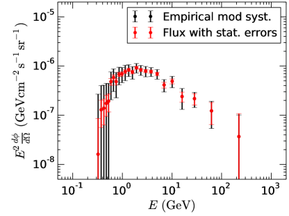
Figure 1: Galactic Centre Excess spectrum, together with statistical and systematical errors, averaged over the ROI $2\degree<|b|<20\degree$ and $|l|<20\degree$. Data and errors are taken from [55].

For calculating the $\gamma$-ray flux for Reticulum II, we use the value of the ‘total’ J-factor, defined as $J_{tot}=\int J(\theta)d\Omega$, found from the Jeans analysis [54]. The value used is $J_{tot}=10^{19.6}$ $\rm{GeV^{2}.cm^{-5}}$, obtained on integration over the ROI $\Delta\Omega=2.4\times 10^{-4}\rm{sr}$ corresponds to the angular radius $0.5\degree$.

Till very recently, excess in the 1 - 10 GeV range was claimed by observations using the so-called Pass 7 data from Reticulum II [24]. Beyond about 10 GeV, the error is too large for any meaningful fit. While such announcements generated considerable activity towards fitting such excess in terms of DM models including the MSSM [8, 42], the later analyses, in terms of the Pass 8 data, disavowed such claims [25, 26]. Upper limits on the flux in the aforesaid range continued to exist, side by side with comparable limits from other dwarf spheroidal galaxies.

Fig. 2 shows the $\gamma$-ray excess upper-limit according to the Pass 8 data. In our subsequent fits, carried out for the GC excess, consistency with the upper limits from Reticulum II Pass 8 data is ensured throughout.

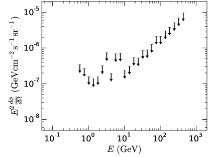
Figure 2: Reticulum II $\gamma$-ray excess upper limit (Pass 8 data) [25, 26]

.

3 Scheme of analysis

3.1 Constraints on the MSSM parameter space

In order to examine the candidature of the lightest neutralino ($\chi^{0}_{1}$) as DM constituent, one has to scan over a reasonable region of the MSSM parameter space, spanned by quantities which can have a bearing on signals related to its annihilation, direct detection etc. The MSSM spectrum has been generated using SuSpect 2.41 [56]. The viability of the region thus examined depend on consistency with the following issues.

• Higgs mass:
  As per observation, we almost certainly have a spin-zero neutral object with mass close to 125 GeV [57, 58]. Keeping this in mind, we have confined ourselves to those regions which yield the mass of lightest neutral scalar $h$ in the range $122~{}\rm{GeV}\leq m_{h}\leq 128~{}\rm{GeV}$. This is conservative range, accounting for theoretical uncertainties [59].

• Constraints from accelerator data:
  The LEP lower limit on the lighter chargino ($\chi^{\pm}_{1}$) [60, 61] has been used to start with. Furthermore, consistency with Higgs search results at LEP leads to allowed regions in the $\mu-M_{2}$ space [62], where $\mu$ and $M_{2}$ are the Higgsino mass parameter and the SUSY-breaking $SU(2)$ gaugino mass parameter respectively. We have only scanned regions that are consistent with this constraint. The masses of sleptons are similarly constrained by LEP [63]. Thus, while a part of our analysis holds all sleptons at high values, we have also included the light-$\tilde{\tau}_{1}$ scenario which may lead to co-annihilation of the DM candidate.

  LHC data impose model-independent lower bounds most markedly on strongly interacting superparticles. Taking these into account, we have kept the gluino and first two family squark masses above 2 TeV [64, 65, 66, 67], and chosen benchmark values accordingly. In any case, the snapshot values thus used do not affect DM-related issues significantly. An exception is the stop mass(es), which can be as low as 150 GeV according to the current data [65, 68, 69]. Consistently with this, and also with the observed Higgs mass, we have included sample scenarios where one of the stops is lighter than the rest of the strongly interacting superparticles, but not so light as to reduce the relic density below admissible limits.

  Light sbottom scenarios, on the other hand, mostly require the $\chi^{0}_{1}$ mass to be at least about 350 GeV [70, 65]. However, this shifts astrophysical $\gamma$-ray peaks to higher frequency regions than what is, for example, observed from the galactic centre. Therefore, such a scenario is not taken account here.

  In addition, low-energy and flavour constraints have been followed at the level of spectrum generation. This includes the contributions to rare B-decays, muon anomalous magnetic moment etc.

• Relic density constraint
  The Planck observations suggest that the relic density lies in the range [9]

  $$\Omega h^{2}=0.1199\pm 0.0022$$ (3.1)

  Accordingly, the contribution from the $\chi^{0}_{1}$ DM candidate can be computed and compared, for which we have used the package micrOMEGAs 4.3.1 [71, 72] .

  However, there are also theoretical uncertainties, typically on the order of 10%, in computing the MSSM DM relic density, which is approximately six times the uncertainty in the observed data [10, 11, 12]. The main source of the former is strong corrections to the annihilation rate, where the dependence on the renormalisation and factorisation scales can be significant. Accordingly, a larger window of the computed value of $\Omega h^{2}$ may be taken as ‘allowed’, leading to the range $\Omega h^{2}=0.12\pm 0.012$.

  Most recent studies have treated only the upper limit on the relic density as a serious constraint. However, when one is examining the viability of the MSSM, it makes sense to assume that the $\chi^{0}_{1}$ the only DM candidate, and that there is no additional new physics around the SUSY breaking scale. Regions of the parameter space that leads to values of $\Omega h^{2}$ considerably smaller than 0.108 are therefore difficult to accept as consistent with the MSSM. We find that this requirement worsens the status of the MSSM as a fit to the $\gamma$-ray observations.

• The co-annihilation region
  As has been mentioned above, one may have a phenomenologically consistent MSSM spectrum with, for example, the lighter stau [73] close in mass to the lightest neutralino. This leads to the well-studied co-annihilation region so long as the mass difference is within 4% [72].

  In our context, when one is in the co-annihilation region, the dominant channel of DM annihilation, which leads to its freeze-out, is different from the pair-annihilation channels which give rise to astrophysical $\gamma$-rays. Therefore, the relic density constraint used in the fit of the $\gamma$-ray data becomes different for such regions. This difference has not been taken into account in erstwhile studies. We have, therefore, separately included co-annihilation regions with the associated relic density constraints in our analysis.

• Direct search constraints
  The most stringent limits on the spin-independent cross-section of $\chi^{0}_{1}$-nucleon scattering can be derived from the XENON1T results [2]. In most of what follows, regions of the parameter space scanned to fit the $\gamma$-ray data have been filtered through this constraint. As before, micrOMEGAs 4.3.1 with most parameters at default values has been used to compute the spin-independent cross-sections.

  Later in the paper, we have taken the following approach, too: the best-fit regions from the analysis of $\gamma$-ray signals/limits from the GC and also dwarf spheroidal galaxies have been obtained without any bias from direct search experiments. The 95.6% C..L. regions have then been subjected to the constraints by the XENON1T data. We interpret the difference of the two kinds of results in section 6

3.2 Benchmarks

As has been stated above, we have fixed the strongly interacting superparticle masses (except that of the stop) at values above 2 TeV. The masses of sleptons in the first two families are similarly fixed [74]. Keeping with the regions that reproduce the lighter neutral scalar mass in the right band, we have varied the following quantities as free parameters:

$M_{1},M_{2},\mu,m_{A}$,

where $M_{1}$ and $M_{2}$ are the $U(1)$ and $SU(2)$ gaugino masses, $\mu$ is the Higgsino mass parameter and $m_{A}$ is the neutral pseudoscalar mass. $\tan\beta$, the ratio of the vacuum expectation values (vev) of the two Higgs doublets, have been fixed at ‘snapshot values’ 5, 20 and 50. The remaining electroweak parameters, it has been checked, do not affect our conclusions significantly.

Four representative MSSM spectra have been considered, which broadly capture various features of DM annihilation, be it in $\gamma$-ray sources or in the early universe. These are

1. All squarks and sleptons above 2 TeV. We call this the heavy squark and slepton (HSS) scenario.

2. Only the lighter stop with a lower mass ($\approx$ 300 GeV), consistently with the Higgs mass and the admissible relic density band. This is the light stop (LST) scenario.

3. Only the lighter stau close enough to the neutralino dark matter candidate, so as to cause co-annihilation. This is called the stau co-annihilation (STC) scenario.

4. The lighter stop with low mass and also a stau in the co-annihilation region. We call this the light stop and stau co-annihilation (LSTSTC) scenario.

The four free parameters mentioned above have been varied over the following ranges: -1000 GeV $<M_{1}<$ 1500 GeV, -1000 GeV $<M_{2}<$ 1500 GeV, -1000 GeV $<\mu<$ 1500 GeV. Depending on the LHC constraints we varied $m_{A}$ in the range 350 GeV - 4000 GeV for $\tan\beta=5$, 450 GeV - 4000 GeV for $\tan\beta=20$, 850 GeV - 4000 GeV for $\tan\beta=50$ [75, 76].

In Table 2, we list the benchmark values for the fixed parameters for the various scenarios listed above. Most of the entries can be justified from the above discussion. In the case of the stop, the SUSY-breaking mass parameters for the $SU(2)$ doublet and singlet components have been separately shown, since they have a bearing of the lighter neutral scalar mass. The corresponding mass eigenstates have been appropriately used, since they are relevant for the $t\bar{t}$ annihilation channel in the LST and LSTSTC scenarios. The trilinear SUSY-breaking parameter $A_{t}$ is fixed at such values as to correctly reproduce the observed Higgs mass, but ensuring consistency with a charge-and color-preserving vacuum, and a potential bounded from below. Lower values of $A_{t}$ necessitate larger $\mu$ or stop mass parameters, which, for these two scenarios, worsen the fits to the $\gamma$-ray data, thereby reducing the regions of good MSSM fit.

Case no	$tan\beta$	$m_{\widetilde{t_{R}}}$(GeV)	$m_{\widetilde{Q_{3}}}$(GeV)	$A_{t}$(GeV)	$m_{\widetilde{\tau_{1}}}$(GeV)
1a	20	2000 GeV	3000	-3000	2500
1b	50	2000 GeV	3000	-3000	2500
1c	5	4000 GeV	4000	-4000	2500
2a	20	300 GeV	4000	-4000	2500
2b	50	300 GeV	4000	-4000	2500
2c	5	300 GeV	4000	-4000	2500
3a	20	2000 GeV	3000	-3000	1.03 $m_{\chi}$
3b	50	2000 GeV	3000	-3000	1.03 $m_{\chi}$
3c	5	4000 GeV	4000	-4000	1.03 $m_{\chi}$
4a	20	300 GeV	4000	-4000	1.03 $m_{\chi}$
4b	5	300 GeV	4000	-4000	1.03 $m_{\chi}$

Table 2: List of various cases we have studied, along with the values of the fixed parameters. All other slepton masses are at 2.5 TeV, All other squark masses are at 3 Tev, gluino mass is at 3 TeV, $A_{b}$ = 4 TeV

3.3 Methodology

We go in the following steps in our analysis:

1. For each of the four scenarios listed in the previous section, we scan over the free parameters, holding the others at their benchmark values as listed in Table 2.

   We implement a Markov Chain Monte Carlo (MCMC) technique to estimate the posterior distribution of our model parameters. We use a publicly available affine-invariant MCMC code EMCEE (Foreman-Mackey et al. 2012) [77], which has considerable performance advantage over other standard MCMC sampling algorithms (Goodman & Weare 2010).

   We start with an ensemble of random walkers ($N_{\rm walker}$), each with a chain length of $N_{\rm step}$, scanning over the model parameter space in their aforementioned ranges. As each walker progresses through the available parameter space, we compute the new posterior probability density and compare it with the old one. Based on their acceptance ratio, the Markov chains gradually converge to a stationary distribution with highest probability (i.e. minimum $\chi^{2}$). The mean and corresponding uncertainty of each parameter are finally computed from the posterior distribution. To ensure the convergence of the chain, we have used $N_{\rm walker}=400$ and $N_{\rm step}=1000-2000$ i.e. a total of $400000-800000$ independent samplings, which is large enough considering the usual mean autocorrelation time.

2. Each point in the parameter space scanned is subjected to the constraints from accelerator experiments, relic density (both lower and upper limits) and direct searches, as discussed above.

3. A likelihood analysis is carried out using the GC excess, consistently with the Reticulum II Pass 8 limits. The likelihood function used in our analyses is given by ${\cal L}\propto\exp(-\chi^{2}/2)$. The expression for $\chi^{2}$ is

   $$\chi^{2}=\sum_{i,j=1}^{24}(\phi_{i}-\overline{\phi_{i}})(\Sigma^{-1})_{ij}(\phi_{j}-\overline{\phi_{j}})$$ (3.2)

   where $\overline{\phi_{i}}$ and is the observed flux from GC, $\phi_{i}$ being the corresponding calculated $\gamma$-ray flux. For GC, the indices $i,j$ denote the energy bin numbers that run from 1 to 24. Once more, the calculation of ${\phi_{i}}$ has been done in micrOMEGAs 4.3.1, interpolating the numerical results contained in files generated from Pythia [78].

   The covariance matrix $\Sigma$ which has a non-diagonal nature in the case of GC excess, is defined as (following eq.5.2 and corresponding description in [20])

   $$\Sigma_{ij}=\Sigma^{emperical}_{ij}\quad+\quad\delta_{ij}(\sigma^{stat}_{i})^{2}\quad+\quad\delta_{ij}(\overline{\phi_{i}}\sigma)^{2}$$ (3.3)

   As defined in [20], $\Sigma^{emperical}_{ij}$ is the covariance matrix for empirical model systematics and $\sigma^{stat}_{i}$ is the statistical error. We have used [55] for obtaining the covariance matrices, statistical errors and the excess data. The entries in $\Sigma^{empirical}_{ij}$, diagonal as well as non-diagonal, arise due the correlation among excesses in different bins, induced in the process of background elimination. Following the argument of [14], we have also added a theoretical uncertainty at the level of $\sigma=10\%$ (last part of eq. 3.3).

   As has been already mentioned, only the upper limits on the flux from Reticulum II following the Pass 8 data [25, 26] are used to constrain regions in the MSSM parameter space. In addition, the consistency with the M31 data [43] is ensured, especially in the frequency range mentioned in the introduction. We also check that the upper limits on the flux from the other dwarf spheroidal galaxies are satisfied. The last-mentioned constraint is not in general difficult to satisfy in our treatment of the Reticulum data, as the J-factor in each such case is smaller than that for Reticulum II [26].

4. The aforementioned procedure yields not only the best-fit value of each of our free parameters, but also the 95.6% C.L. region in the hyperspace spanned by them. From this one obtains various two-parameter marginalised plots, for the basic parameters as well as derived quantities such as physical masses.

5. The overall frequency distributions corresponding to our 95.6% C.L. bands are compared with the observed GC excess distribution. A comparison with the constraints from Reticulum II is also made.

Finally, we compare the above results with the alternative analysis as outlined at the section 6.

4 Results

we now present the results of our analyses for the various benchmark scenarios listed in (Table 2). All Higgs and MSSM particle masses, widths, cross sections etc. have been calculated at the one-loop level. While most relevant parameters are scanned over, the benchmark spectra correspond to ’snapshot values’ of $\tan\beta$, so that the results have a generic nature, representative of all relevant kinds of MSSM spectra that can have distinctive roles in DM annihilation. The values of $\chi^{2}$ per degree of freedom for all the benchmarks have been shown in Table 3.

4.1 Case 1: HSS

This is the scenario where all sleptons and squarks masses have high values ($>$ 2 TeV).

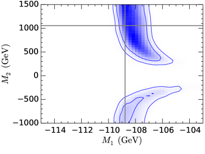
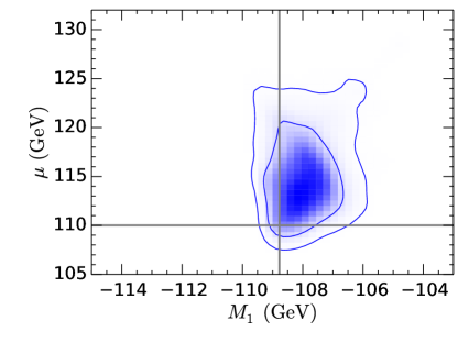
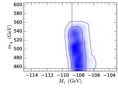
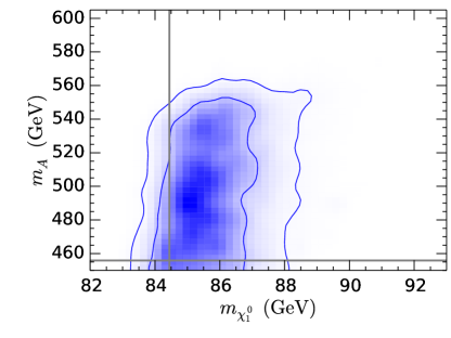
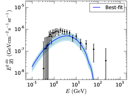
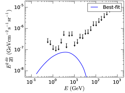
Figure 3: 1$\sigma$ and 2$\sigma$ contours plots in the plane of $M_{1}-M_{2}$ (top left), $M_{1}-\mu$ (top right), $M_{1}-m_{A}$ (middle left), $m_{\chi^{0}_{1}}-m_{A}$ (middle right) for Case 1a. Solid gray lines indicate the best fit values. Bottom left: 2$\sigma$ bands of GC excess spectrum (light blue region) correspond to this case along with Fermi-LAT GC excess data and error bars (diagonal part of the covariance matrix). Deep blue line is the spectrum for best-fit points. Bottom right: Reticulum II $\gamma$-ray spectrum for the best-fit point (blue curve) along with the upper-limit on flux from Pass 8 analysis.

Case 1a: Among all the scenarios sampled, this case fits the GC excess spectrum best. The best-fit point corresponds to $M_{1}=-108.75,M_{2}=1115.85,\mu=110.30,m_{A}=451.92$, with $\chi^{2}_{min}=51.3$ for DOF = 24. The 2D projection of the $1\sigma$ and $2\sigma$ contour plots in the parameter hyperspace, corresponding to the fit to the GC flux constrained by Reticulum II data, are shown in Fig. 3. This yields marginalised plots in various pairs of parameters, as will also be seen in the cases to follow. Here $M_{2}$ is less tightly constrained. The area thus marked out yields the lightest neutralino mass ($m_{\chi^{0}_{1}}$) in the range $\simeq$ 83 - 88 GeV, and it is largely Bino, with some Higssino admixture. In any case, since we are imposing the direct DM search constraint, the lightest neutralino cannot have a very large Higgsino component. The dominant channel of annihilation in this case is mainly $W^{+}W^{-}$, along with a small but perceptible branching fraction for $b\bar{b}$. For $tan\beta=20$, the LHC lower limit on $m_{A}$is about 450 GeV. The favoured range emerging from our $2\sigma$ fit is $m_{A}\simeq$ 450 - 560 GeV. This basically weakens the resonant annihilation channel into third family fermion pairs, namely, $\chi^{0}_{1}\chi^{0}_{1}\rightarrow f\overline{f}$, for low neutralino masses, as required for matching the GC $\gamma$-ray spectrum.

The limit on $m_{A}$ for $\tan\beta=5$ is lower, but the $b\bar{b}$ coupling is weaker when $m_{h}$ is fixed at the observed value. For $\tan\beta=50$, the corresponding limit goes up to $\simeq$ 850 GeV.

The annihilation in the $W^{+}W^{-}$ channel is facilitated for such spectrum by the fact that $\chi_{1}^{\pm}$, the lighter chargino has a substantial Higgsino component, since $\mu$ is on the smaller side. The close proximity of $\mu$ and $M_{1}$, while complying with the lowers limits on the chargino mass, enhances the t-and u-channels of annihilation, which interfere constructively. However, in the context of the early universe, a boost in such annihilation rate implies correspondingly high $\left\langle\sigma v\right\rangle$, averaged thermally. The lower bound on the relic density, modulo the aforementioned uncertainties, therefore restricts the annihilation rate. This cannot be ameliorated by higher neutralino and chargino masses, since that shifts the peak of the GC $\gamma$-ray distribution to relatively high frequencies where the observed rate is exceeded. A strict adherence to the lower limit on the relic density (as one must do if the MSSM is the only new physics) thus implies that, with the required low $m_{\chi^{0}_{1}}$, one cannot achieve as much DM annihilation rate as is required to fully explain the GC $\gamma$-ray excess with the observed frequency distribution. In Fig. 3 we have presented the $2\sigma$ band of the predicted GC excess spectrum along with the data points. We re-iterate that the band does not give sufficient saturation to the data as $\left\langle\sigma v\right\rangle$ is constrained by the relic density lower bound. Fig. 3 shows the Reticulum II $\gamma$-ray spectrum for the best-fit model in this case, where consistency with the Pass 8 limits is obvious.

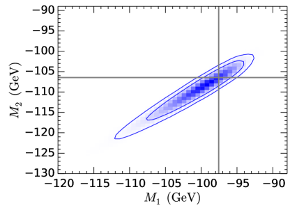
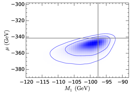
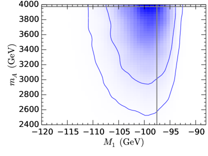
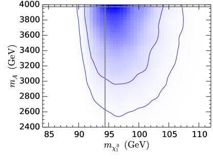
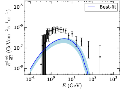
Figure 4: 1$\sigma$ and 2$\sigma$ contours plots in the plane of $M_{1}-M_{2}$ (top left), $M_{1}-\mu$ (top right), $M_{1}-m_{A}$ (middle left), $m_{\chi^{0}_{1}}-m_{A}$ (middle right) for Case 1b. Solid gray lines indicate the best fit values. Bottom left: 2$\sigma$ bands of GC excess spectrum (light blue region) correspond to this case along with Fermi-LAT GC excess data and error bars (diagonal part of the covariance matrix). Deep blue line is the spectrum for best-fit points. Bottom right: Reticulum II $\gamma$-ray spectrum for the best-fit point (blue curve) along with the upper-limit on flux from Pass 8 analysis.

Case 1b: The fits for this case yield $\chi^{2}_{min}=65.1$, with the same DOF as in the previous case. The best-fit point corresponds to $M_{1}=-97.56,M_{2}=-106.45,\mu=-341.44,m_{A}=3973.12$. Once more, the dominant channel of annihilation in this case is $\chi^{0}_{1}\chi^{0}_{1}\rightarrow W^{+}W^{-}$. The $2\sigma$ contour plots corresponding to the fitting of GC flux excess and Reticulum II upper limits is shown in Fig. 4. The range of neutralino mass in the $2\sigma$ contours for this case comes out to be in the range $\simeq$ 90 - 108 GeV. The relatively low best-fit value of $M_{2}$ and a somewhat higher $\mu$ leads to a $\chi^{0}_{1}$ that is mostly Bino, with a smaller admixture of Wino. For $tan\beta=50$, as used here, $m_{A}$ comes out to be in the range $\simeq$ 2500 - 4000 GeV. This, together with the negligible Higgsino component in $\chi^{0}_{1}$, seals the fate of the resonant annihilation channel and thus prevents the relic density from becoming too low. On the other hand, the small mass difference between $\chi_{1}^{\pm}$ and $\chi_{1}^{0}$ once more drives the $W^{+}W^{-}$ channel. Fig. 4 shows the 2$\sigma$ band of the GC excess spectrum drawn as earlier. As already discussed for the previous case, the lower limit on the relic density in conjunction with the position of the peak of the GC spectrum restricts the quality of the fit for MSSM. The conclusion is similar for the other benchmark scenarios discussed below, and we do not repeat this statement for these cases.

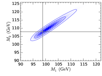
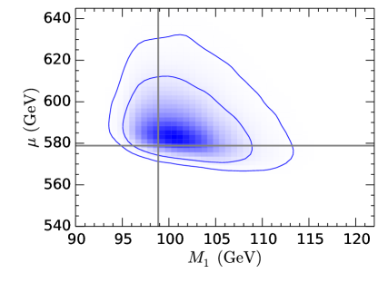
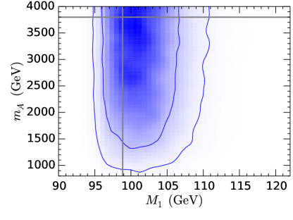
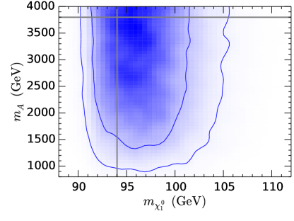
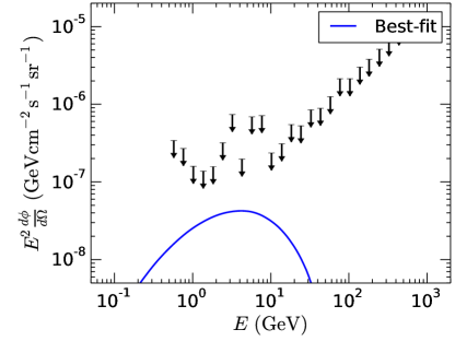
Figure 5: 1$\sigma$ and 2$\sigma$ contours plots in the plane of $M_{1}-M_{2}$ (top left), $M_{1}-\mu$ (top right), $M_{1}-m_{A}$ (middle left), $m_{\chi^{0}_{1}}-m_{A}$ (middle right) for Case 1c. Solid gray lines indicate the best fit values. Bottom left: 2$\sigma$ bands of GC excess spectrum (light blue region) correspond to this case along with Fermi-LAT GC excess data and error bars (diagonal part of the covariance matrix). Deep blue line is the spectrum for best-fit points. Bottom right: Reticulum II $\gamma$-ray spectrum for the best-fit point (blue curve) along with the upper-limit on flux from Pass 8 analysis.

Case 1c: One obtains $\chi^{2}_{min}$ = 65.2 for this case, reflecting the fact that both this case and the previous one yield worse fits compared to Case 1a. The combination of parameters corresponding to the best fit are $M_{1}=98.85,M_{2}=107.87,\mu=578.89,m_{A}=3798.42$, and the major annihilation channel once more is $W^{+}W^{-}$. Fig. 5 contains the 2$\sigma$ contour plots for this case. At 95.6$\%$ C.L., the neutralino mass lies in the range $\simeq$ 90 - 105 GeV and is composed of Bino and Wino as above. Here one ends up with a high-mass $m_{A}$ which is in the range 800 - 4000 GeV. Once more, the 2$\sigma$ band of the GC excess spectrum and the best fit Reticulum II spectrum predicion for the best-fit model are shown in Fig. 5. In this case, too, the lower limit on the relic density restricts large $\left\langle\sigma v\right\rangle$ and low $m_{\chi}$, so that the GC $\gamma$-ray data cannot fitted in a completely satisfactory manner.

4.2 Case 2: LST

In this scenario we have set the right-chiral stop mass parameter $m_{\tilde{t_{R}}}$ at 300 GeV and retained other squarks and sleptons above 2 TeV. The latter choice, as has been mentioned already, is not seen to affect the fits appreciably. The bigger mass parameters (including the A-parameters corresponding to the trilinear soft SUSY breaking terms) are varied in such a way as to reproduce the lighter neutral scalar mass in the appropriate band. This keeps the lighter stop around $\sim$ 260 - 300 GeV for all benchmark points. For higher values of the lighter stop mass eigenstate than 300 GeV, the existing collider constraints would force us to a heavier $\chi^{0}_{1}$ [65, 68, 69] and as a result the fitting of $\gamma$-ray data would be worse. Values lower than 260 GeV for $m_{\tilde{t_{R}}}$, on the other hand, can create problems with the Higgs mass when one tries to maintain consistency with other constraints on MSSM spectra.

In principle, it may be curious to check the implications of scenarios with other third family sfermions like the sbottom or the stau as well. For a light sbottom, however, the lower limit on the lightest neutralino is higher than in the case of a light stop [70, 65], thus worsening the GC $\gamma$-ray fits. The case of a light stau can make a noticeable difference only when it is close enough to the $\chi^{0}_{1}$ to co-annihilate, a case that has been reported separately below.

As in the HSS scenario, here, too, we shall consider the results with three snapshot values of $\tan\beta$. However, we begin by pointing out a few salient features that are common to all three cases.

• The candidature of a light stop in our context thrives on the $t\bar{t}$ channel of annihilation. The subprocesses include the pseudoscalar-mediated s-channel diagram as well as the stop-mediated t-and u-channel ones.

• The $t\bar{t}A$ couping is proportional to $\cot\beta$, thus making the s-channel dominate in the annihilation process for $\tan\beta$ = 5. As for the top-stop-$\chi^{0}_{1}$ interaction, $\tan\beta$ enters in two ways: via the coupling to the Higgsino component, and through the neutralino mass matrix itself. The final results are related to all of these factors, and also to the fact that the t-and u-channels interfere destructively.

• In order to annihilate into a top-antitop pair, one requires $m_{\chi^{0}_{1}}\geq$ 175 GeV approximately, a requirement that comes from the LHC constraints on the $m_{\chi^{0}_{1}}-m_{\tilde{t}_{1}}$ plane [65, 68, 69]. However, this inevitably tends to shift the peak of the GC $\gamma$-ray spectrum to the region of higher frequency than where the observed peak lies. This, together with the limit on upward scaling of the profile coming from the requirement of a minimum relic density, poses a challenge to good fits of all data in the light stop scenario.

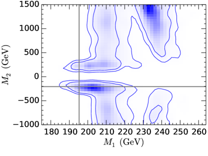
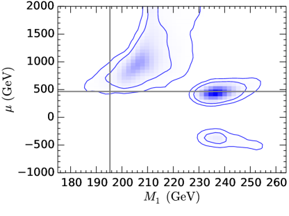
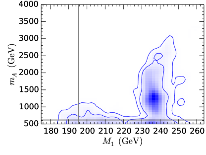
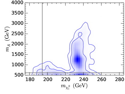
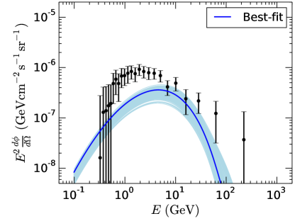
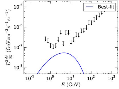
Figure 6: 1$\sigma$ and 2$\sigma$ contours plots in the plane of $M_{1}-M_{2}$ (top left), $M_{1}-\mu$ (top right), $M_{1}-m_{A}$ (middle left), $m_{\chi^{0}_{1}}-m_{A}$ (middle right) for Case 2a. Solid gray lines indicate the best fit values. Bottom left: 2$\sigma$ bands of GC excess spectrum (light blue region) correspond to this case along with Fermi-LAT GC excess data and error bars (diagonal part of the covariance matrix). Deep blue line is the spectrum for best-fit points. Bottom right: Reticulum II $\gamma$-ray spectrum for the best-fit point (blue curve) along with the upper-limit on flux from Pass 8 analysis.

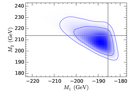
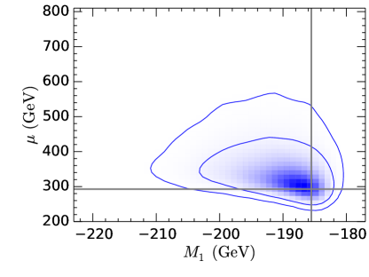
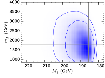
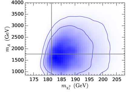
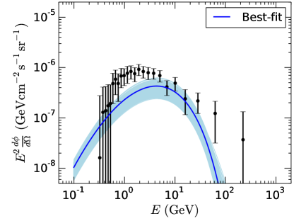
Figure 7: 1$\sigma$ and 2$\sigma$ contours plots in the plane of $M_{1}-M_{2}$ (top left), $M_{1}-\mu$ (top right), $M_{1}-m_{A}$ (middle left), $m_{\chi^{0}_{1}}-m_{A}$ (middle right) for Case 2b. Solid gray lines indicate the best fit values. Bottom left: 2$\sigma$ bands of GC excess spectrum (light blue region) correspond to this case along with Fermi-LAT GC excess data and error bars (diagonal part of the covariance matrix). Deep blue line is the spectrum for best-fit points. Bottom right: Reticulum II $\gamma$-ray spectrum for the best-fit point (blue curve) along with the upper-limit on flux from Pass 8 analysis.

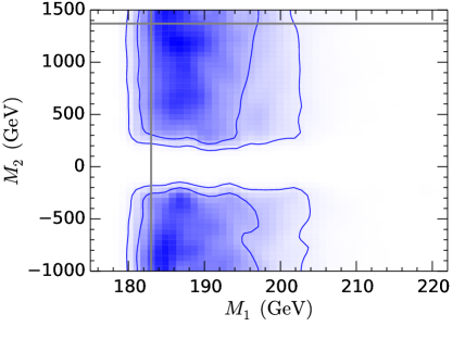
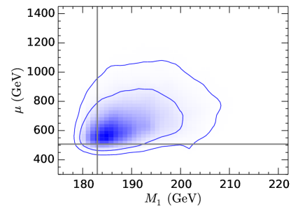
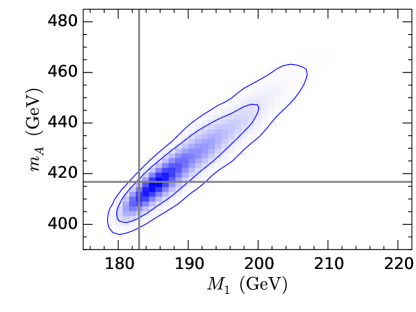
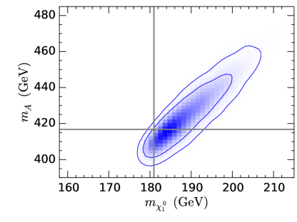
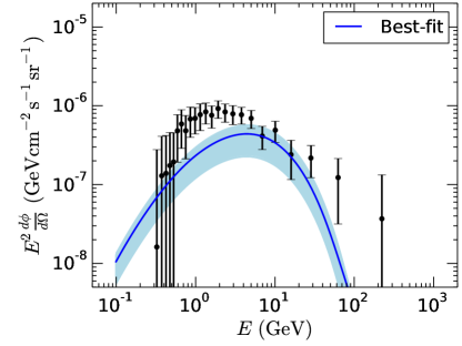
Figure 8: 1$\sigma$ and 2$\sigma$ contours plots in the plane of $M_{1}-M_{2}$ (top left), $M_{1}-\mu$ (top right), $M_{1}-m_{A}$ (middle left), $m_{\chi^{0}_{1}}-m_{A}$ (middle right) for Case 2c. Solid gray lines indicate the best fit values. Bottom left: 2$\sigma$ bands of GC excess spectrum (light blue region) correspond to this case along with Fermi-LAT GC excess data and error bars (diagonal part of the covariance matrix). Deep blue line is the spectrum for best-fit points. Bottom right: Reticulum II $\gamma$-ray spectrum for the best-fit point (blue curve) along with the upper-limit on flux from Pass 8 analysis.

Case 2a: For this case, the best fit point corresponds to $M_{1}=195.32,M_{2}=-205.55,\mu=464.85,m_{A}=617.18$, with $\chi^{2}_{min}$ = 65.7 for DOF = 24, and the DM mass in the range $\simeq$ 180 - 260 GeV at 95.6$\%$ C.L. The aforementioned trend of upward movement of the GC $\gamma$-ray peak in the LST scenario causes more mismatch with data if $\left\langle\sigma v\right\rangle$ goes to the higher side. This favours values of $m_{A}$ which are always above 600 GeV.

As before, Fig. 6 demonstrates the viability of the preferred regions with respect to the GC excess spectrum and the observations on Reticulum II.

Case 2b: This is the second best case (after Case 1a) for fitting the GC excess, with $\chi^{2}_{min}$ = 61.2. The best fit point corresponds to $M_{1}=-185.52,M_{2}=213.8,\mu=292.79,m_{A}=1769.64$, the lightest neutralino mass being in the range $\simeq$ 178 - 205 GeV at 95.6$\%$ C.L. Fig. 7 includes the 2$\sigma$ contour plots. This is a situation where the s-channel annihilation diagram is least significant. This is also because the favoured values of $m_{A}$ are high for $\tan\beta$ = 50.

The contribution to annihilation comes from stop mediated t-channel annihilation, yielding also a relic density in the right range. Our earlier observations related to the GC spectrum hold here as well, and the comparison with data for GC as well as Reticulum II are found in Fig. 7.

Case 2c: With $\tan\beta$ = 5, this is the case where the pseudoscalar-mediated s-channel annihilation dominates. The best fit point corresponds to the parameter values $M_{1}=182.99,M_{2}=1369.44,\mu=507.05,m_{A}=416.75$, with $\chi^{2}_{min}$ = 62.2. The lightest neutralino mass at 95.6$\%$ C.L. comes out to be in the range $\sim$ 175 - 210 GeV. Fig. 8 represents the 2$\sigma$ contour plots for this case. For this value of $\tan\beta$, $m_{A}$ can be as low as 350 GeV. However, the fact that $m_{\chi_{1}^{0}}$ must be at least equal to $m_{t}$ pushes the lowest value of $m_{A}$ so close to resonance that the annihilation rate overshoots the upper limit imposed by the requirement of a minimum relic density. In addition, this also leads to the previously mentioned problem in fitting the GC $\gamma$-ray spectrum. Thus the 2$\sigma$ minimum in the marginalised plot involving $m_{A}$ does not go below $m_{A}=400$ GeV approximately. Figs. 8, drawn as before, are self-explanatory.

4.3 Case 3: STC

We consider next the stau co-annihilation region, where the lighter stau and lightest neutralino masses are within 3$\%$ of each other. All other slepton and squark masses are set at values ($>$ 2 TeV). The existing lower limits on the stau mass from the LEP and LHC data [73] have been respected throughout our analysis. Obviously, the $\chi_{1}^{0}$ mass, too, get constrained in a correlated fashion. We remind the reader here that such co-annihilation regions bring in additional angles when it comes to the neutralino freeze-out process, and thus may cause modification in the relic density constraints. However, the DM annihilation process in the GC, dwarf spheroidal galaxies or even galactic clusters is solely of the form $\chi_{1}^{0}\chi_{1}^{0}\rightarrow X\bar{X}$, as the co-annihilation partner is not available there.

In principle, one can also think of MSSM spectra with the $\chi^{\pm}_{1}$ or the lighter stop/sbottom as the co-annihilation partner of the $\chi_{1}^{0}$. Of these, the possibility of coannhilation with $\chi^{\pm}_{1}$ is implicitly included in all of our scans. With stop co-annihilation, only a limited region in the LST scenario, already included in our analysis, can be effective. However, as we have already observed, these almost always require the neutralino to be of such mass where the $\gamma$-ray distribution become peaked at somewhat high values compared to what is indicated by the data. This problem is more pronounced for sbottom co-annihilation, since the sbottom mass has still higher bounds, as has been mentioned above.

A feature of the STC scenario is that the $\chi_{1}^{0}$ pair-annihilation cross section can have a more substantial branching fraction in the $\tau^{+}\tau^{-}$ final state, driven by either the $A_{0}$ in s-channel or the lighter stau in the t/u-channel . The $\gamma$-ray energy spectrum is affected accordingly.

The fits obtained for the three regions corresponding to STC are in fact worse than those for both HSS and LST. This is because of a two-fold constraint applicable here. Firstly, co-annihilation tends to lower the relic density below the stipulated lower limit. Therefore, if the MSSM has to account for all dark matter, it is imperative to keep the contribution to $\left\langle\sigma v\right\rangle$ in the freeze-out process (as opposed to annihilation within stellar objects) within limits. One is thus forced to go to higher mass regions (as can be seen from [79]) for the $\chi_{1}^{0}-\tilde{\tau_{1}}$ duo, leading again to the undesirable consequence of the $\gamma$-ray peak shifting towards high frequencies.

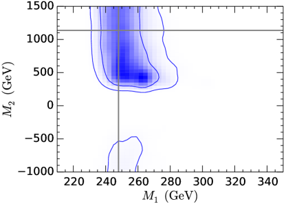
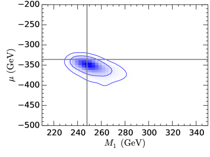
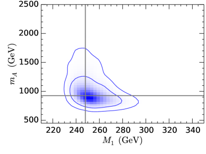
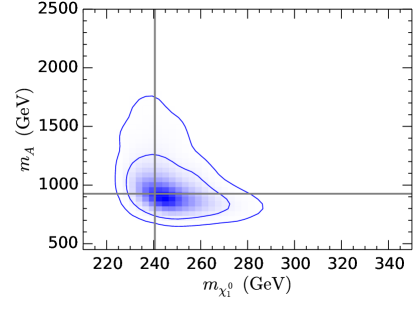
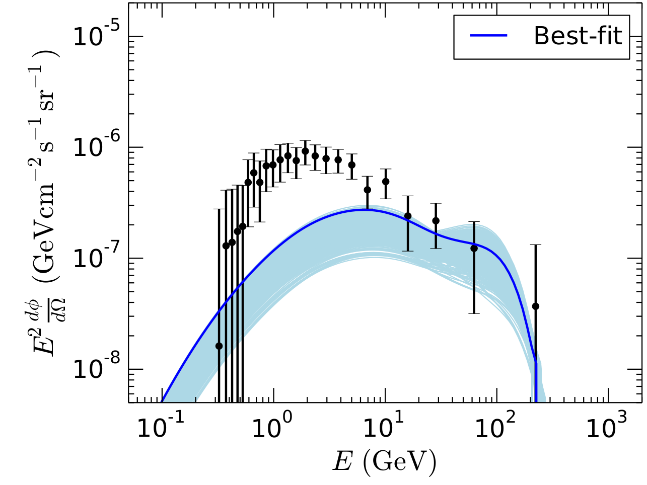
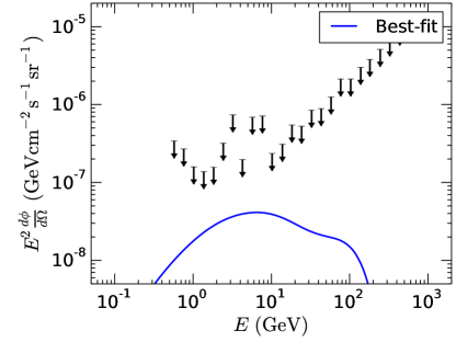
Figure 9: 1$\sigma$ and 2$\sigma$ contours plots in the plane of $M_{1}-M_{2}$ (top left), $M_{1}-\mu$ (top right), $M_{1}-m_{A}$ (middle left), $m_{\chi^{0}_{1}}-m_{A}$ (middle right) for Case 3a. Solid gray lines indicate the best fit values. Bottom left: 2$\sigma$ bands of GC excess spectrum (light blue region) correspond to this case along with Fermi-LAT GC excess data and error bars (diagonal part of the covariance matrix). Deep blue line is the spectrum for best-fit points. Bottom right: Reticulum II $\gamma$-ray spectrum for the best-fit point (blue curve) along with the upper-limit on flux from Pass 8 analysis.

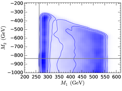
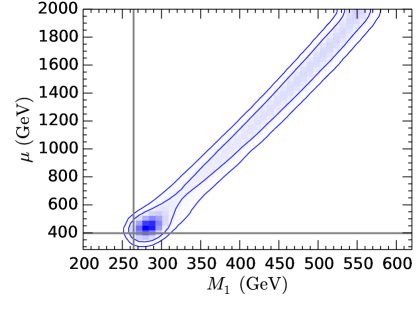
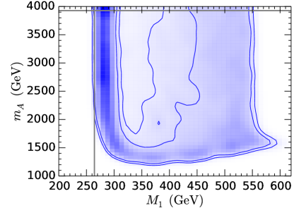
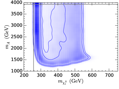
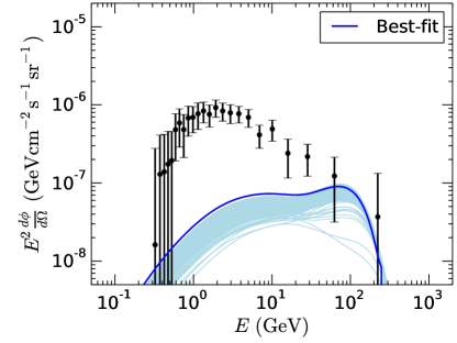
Figure 10: 1$\sigma$ and 2$\sigma$ contours plots in the plane of $M_{1}-M_{2}$ (top left), $M_{1}-\mu$ (top right), $M_{1}-m_{A}$ (middle left), $m_{\chi^{0}_{1}}-m_{A}$ (middle right) for Case 3b. Solid gray lines indicate the best fit values. Bottom left: 2$\sigma$ bands of GC excess spectrum (light blue region) correspond to this case along with Fermi-LAT GC excess data and error bars (diagonal part of the covariance matrix). Deep blue line is the spectrum for best-fit points. Bottom right: Reticulum II $\gamma$-ray spectrum for the best-fit point (blue curve) along with the upper-limit on flux from Pass 8 analysis.

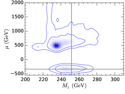
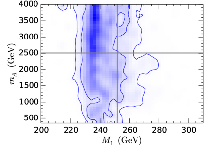
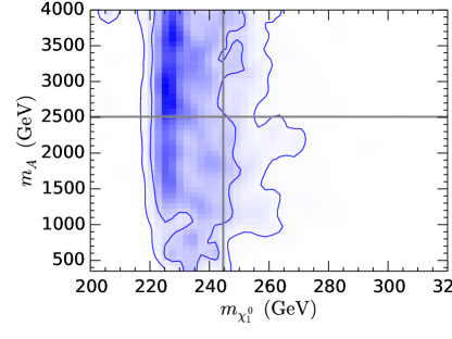
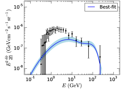
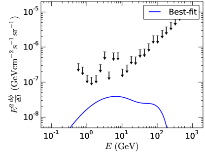
Figure 11: 1$\sigma$ and 2$\sigma$ contours plots in the plane of $M_{1}-M_{2}$ (top left), $M_{1}-\mu$ (top right), $M_{1}-m_{A}$ (middle left), $m_{\chi^{0}_{1}}-m_{A}$ (middle right) for Case 3c. Solid gray lines indicate the best fit values. Bottom left: 2$\sigma$ bands of GC excess spectrum (light blue region) correspond to this case along with Fermi-LAT GC excess data and error bars (diagonal part of the covariance matrix). Deep blue line is the spectrum for best-fit points. Bottom right: Reticulum II $\gamma$-ray spectrum for the best-fit point (blue curve) along with the upper-limit on flux from Pass 8 analysis.

Case 3a: As mentioned already, this case gives a poor fit to the GC excess compared to the previous cases, yielding $\chi^{2}_{min}=85.2.$ for DOF = 24. The best fit point corresponds to $M_{1}=248.0,M_{2}=1136.6,\mu=-335.96,m_{A}=925.58$. $m_{\chi^{0}_{1}}$ is in the range $\simeq$ 220 -285 GeV at 95.6$\%$ C.L. In order to offset the downward pull on the relic density due to co-annihilation, one requires the lightest neutralino to be more massive [79] than in any of the previous cases. The dominant channel of annihilation of DM pairs in GC/Reticulum II is $t\overline{t}$ and $\tau\overline{\tau}$, mediated by the pseudoscalar Higgs. The high mass of the $\chi^{0}_{1}$ will shift the peak to high-frequency regions, and it is only through a sufficiently reduced (co)-annihilation rate that one can be saved from exceeding the observed limits there. The profile, however, will display a clear mismatch with what is observed, making it a rather poor fit. The various 2$\sigma$ contour plots as well as the band attempting a fit to the GC profile and the prediction best GC fit on the Reticulum II spectrum are presented in Fig. 9. As earlier, the GC best fit corresponds to practically no Reticulum excess and thus comply with the Pass 8 upper limits.

Cases 3b and 3c lead to very similar conclusions. For Case 3b, with $\tan\beta$= 50, the $\tau^{+}\tau^{-}$ annihilation channel rises above $t\bar{t}$. The various plots can be seen in Figs. 10 and 11.

4.4 Case 4: LSTSTC

This scenario has the stau co-annihilation region buttressed with one light stop. Most observations here are similar to those made for the STC scenario. However, the requirements brought in by stau co-annihilation during freeze-out tend to jack up $m_{\chi^{0}_{1}}$, with the additional prospect of making it close to the light stop mass. This makes the latter an additional co-annihilation partner for the DM candidate, threatening one with too fast an annihilation rate, and a consequent violation of the lower limit on the relic density. As a result, the parameter space consistent with all constraints shrinks in size, The $\sigma$ contours have to emerge out of whatever is left after eliminating the regions ruled out by the above consideration. Together with the problems arising in the GC spectrum fit, this yields fits at least as bad as those in the previous scenario.

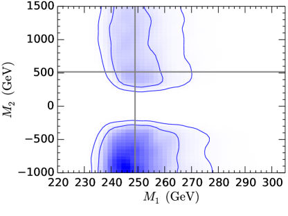
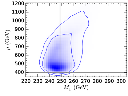
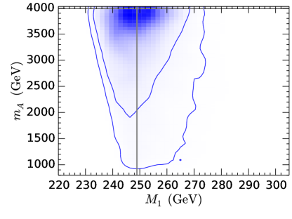
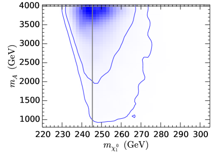
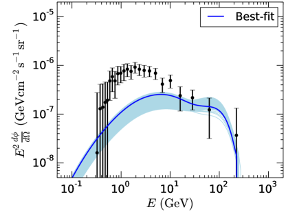
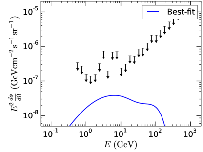
Figure 12: 1$\sigma$ and 2$\sigma$ contours plots in the plane of $M_{1}-M_{2}$ (top left), $M_{1}-\mu$ (top right), $M_{1}-m_{A}$ (middle left), $m_{\chi^{0}_{1}}-m_{A}$ (middle right) for Case 4a. Solid gray lines indicate the best fit values. Bottom left: 2$\sigma$ bands of GC excess spectrum (light blue region) correspond to this case along with Fermi-LAT GC excess data and error bars (diagonal part of the covariance matrix). Deep blue line is the spectrum for best-fit points. Bottom right: Reticulum II $\gamma$-ray spectrum for the best-fit point (blue curve) along with the upper-limit on flux from Pass 8 analysis.

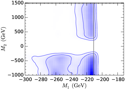
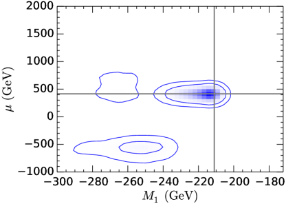
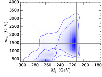
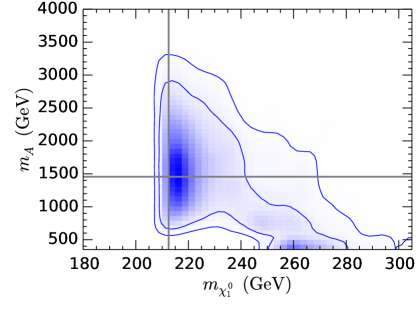
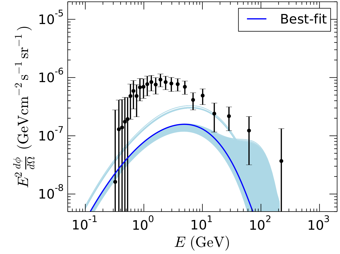
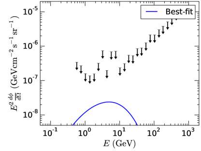
Figure 13: 1$\sigma$ and 2$\sigma$ contours plots in the plane of $M_{1}-M_{2}$ (top left), $M_{1}-\mu$ (top right), $M_{1}-m_{A}$ (middle left), $m_{\chi^{0}_{1}}-m_{A}$ (middle right) for Case 4b. Solid gray lines indicate the best fit values. Bottom left: 2$\sigma$ bands of GC excess spectrum (light blue region) correspond to this case along with Fermi-LAT GC excess data and error bars (diagonal part of the covariance matrix). Deep blue line is the spectrum for best-fit points. Bottom right: Reticulum II $\gamma$-ray spectrum for the best-fit point (blue curve) along with the upper-limit on flux from Pass 8 analysis.

For $\tan\beta$= 5 and 20, the $t\bar{t}$ channel dominates in DM annihilation in the GC as well as dwarf spheroidal galaxies. The tau-pair final state is more competitive for $\tan\beta$= 50, where, however, the fit is far too wayward to present here. The relevant plots are shown in Figs. 12 and 13. We also list in Table 3 the values of $\chi^{2}$/DOF for all the cases discussed above.

The above discussion elicits the following points. First, the viability of any type of MSSM spectrum is crucially governed by the lower bound on the relic density together with the shape of the GC $\gamma$-ray spectrum, together with the latest direct search results. Once the constraints from the above are adhered to, observations related to Reticulum II do not restrict any scenario significantly. And lastly, even the best of all the fits to MSSM listed above lead to somewhat poor $\chi^{2}$/DOF. More will be said on this in section 6.

Case no	$\chi^{2}_{min}$/DOF
1a	51.3/24
1b	65.1/24
1c	65.2/24
2a	65.7/24
2b	61.2/24
2c	62.2/24
3a	85.2/24
3b	97.2/24
3c	87.5/24
4a	85.9/24
4b	80.6/24

Table 3: values of $\chi^{2}_{min}$/DOF for various cases.

5 Radio signal from Coma cluster

DM annihilation inside the galaxies and galaxy clusters can produce high-energy secondary charged particles (mostly electron and positron) in the final state. Upon interaction with the ambient magnetic field, these relativistic particles produce synchrotron radiation which can lead to radio signals [80, 81, 82]. One example of these is the Coma cluster, which has been extensively observed in various frequency ranges [6, 8]. In this section, we compute the radio signal for the DM models we have studied in the earlier sections and compare with the observational data. Note that the comparison with the radio data carried out here does not have any consequences for the constraints obtained on the MSSM parameter space. The radio data points used in these studies have been obtained from [23].

Multi-frequency fits for radio emission from the Coma cluster, in conjunction with the GC and Reticulum II data, have already been reported in the literature [43]. However, such studies have by and large treated the DM mass ($m_{\chi^{0}_{1}}$) and $\left\langle\sigma v\right\rangle$ as independent parameters, adjusting the latter to saturate the radio data from the Coma cluster. The dynamics of neutralino pair-annihilation, to which one is beholden at any point in the MSSM parameter space, is not taken into consideration there.

On the other hand, we have started by fitting the MSSM parameters in details from the GC data where the background is known better. The shape of the $\gamma$-ray spectrum is also used in detail.The channels of annihilation and the net $\left\langle\sigma v\right\rangle$ is computed rather than adjusted for any point in the MSSM parameter space. The phenomenological constraints on MSSM parameters (including the observed Higgs mass), the lower limit on the relic density for MSSM being the only dark matter source, and the direct search constraints on the spectrum are all taken into account. The regions in the parameter space thus available are used to compute the DM annihilation rates and the consequent radio flux from the Coma Cluster.

The synchrotron flux from the Coma cluster depends on the $e^{\pm}$ source function [6, 8]:

$$Q_{e}(r,E)=\left\langle\sigma v\right\rangle\frac{dN_{e}}{dE}\mathcal{N}_{pairs}(r),$$ (5.1)

where $\left\langle\sigma v\right\rangle$ is the same DM annihilation rate we used previously for $\gamma$-ray spectrum calculation (eq. 2.1 and 2.6) and $dN_{e}/dE$ is the number of $e^{\pm}$ produced per annihilation per unit energy. The quantity $\mathcal{N}_{pairs}(r)$ denotes the number of DM particle pairs per unit volume squared at radial distance $r$ of the halo around the cluster. The quantity depends on the DM density profile of the halo (denoted by $\rho(r)$) and the contributions from sub-halos distributed inside the main halo [6, 8]. For the calculation of $\mathcal{N}_{pairs}(r)$ we follow the steps exactly as described in [6].

Using the above source function, the full calculation of radio flux density spectrum $S(\nu)$ as a function of emitted radio frequency $\nu$ is done subsequently, again following [6] and [83]. However, in view of the various uncertainties, we have used two sets of values of the parameters controlling the DM profile, and also the magnetic field, which are described below.

• Model A: In the first case, following reference [6], we have used the N04 profile, with $\alpha=0.17$, and a homogeneous magnetic field of magnitude 1.2 $\mu G$.

  $$\rho_{N04}(r)=\rho_{s}\exp\left[-\frac{2}{\alpha}\left(\left(\frac{r}{r_{s}}\right)^{\alpha}-1\right)\right],\qquad\qquad B_{\mu}=1.2\mu G$$ (5.2)

  Here $\rho_{s}$ is the characteristic density of the halo and $r_{s}$ is the cale radius of the profile.

• Model B: We show the difference in prediction by switching over to the NFW profile in the second case, with slope $\gamma=1$ [84]

  $$\rho_{NFW}(r)=\frac{\rho_{s}}{(\frac{r}{r_{s}})(1+\frac{r}{r_{s}})^{2}}$$ (5.3)

  and a radial magnetic field distribution motivated by observations of Faraday rotation for Coma, as in [8, 85]

  $$B_{\mu}(r)=B_{0}\left(1+\left(\frac{r}{r_{s}}\right)^{2}\right)^{-0.56},\qquad\qquad B_{0}=4.7\mu G$$ (5.4)

The scale radius is taken to be the same in both cases [6, 8]. Our code is calibrated by exactly matching the fluxes given in reference [6].

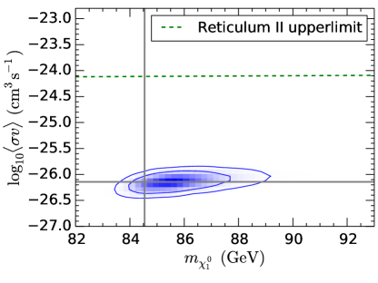
Figure 14: 1$\sigma$ and 2$\sigma$ (blue) contours plots in the plane of dark matter annihilation rate ($\left\langle\sigma v\right\rangle$) vs dark matter mass ($m_{\chi^{0}_{1}}$) for Case 1a. Reticulum II upper limit (from Pass 8 analysis) also has been shown with green dashed line.

The quantity $\mathcal{N}_{pairs}(r)$ (which plays a role similar to the J-factor in eqs. 2.1 and 2.6) is inversely proportional to dark matter mass squared [6]. Consequently the flux normalisation (following equation 5.1) is proportional to $\frac{\left\langle\sigma v\right\rangle}{m_{\chi_{1}^{0}}^{2}}$. Among all the previously described cases, Case 1a, the best from the standpoint of $\gamma$-ray data, has the largest $\frac{\left\langle\sigma v\right\rangle}{m_{\chi_{1}^{0}}^{2}}$. This case is thus expected to yield the highest radio flux. The constraints in the $\left\langle\sigma v\right\rangle$ - $m_{\chi_{1}^{0}}$ plane obtained from the likelihood analysis for this case is shown in Fig. 14. We can see that the allowed range in dark matter mass is quite small and has value around $\sim 85$ GeV. The annihilation cross section peaks close to $10^{-26}$ cm³ s^-1, which is significantly smaller than the upper limit inferred from the Reticulum II data.

In Fig. 15, we have shown the comparison of the observed radio data from Coma cluster [23] with the calculated flux density spectrum ($S(\nu)$) [6, 8] for the best-fit point corresponding to Case 1a (ensuring consistency with M31 data and the Reticulum upper limits), for the two parameter sets discussed above.

Figure 15: Radio flux density spectrum for the Coma cluster for benchmark 1a for two astrophysical parameter sets. The blue dotted and dashed lines, marked as model A and model B, correspond respectively to the N04 and NFW profiles, and the corresponding magnetic fields. The radio data are taken from [23]

It is clear that, even with the relative enhancement of the radio flux in the second case (model B), the best fit curve from the $\gamma$-ray data accounts for at most 20% of this radio signal for $\approx 5$ GHz. The shortfall is considerably more conspicuous for lower frequencies, and also with the first set of model parameters. One possible way of increasing the signal would be to use a higher value of the magnetic field (which in this case turns out to be $\sim 20\mu$G), however, such values would be inconsistent with the Faraday rotation measures [85].

This, however, is not necessarily an inconsistency, since the conventional astrophysical sources of $e^{\pm}$ in the Coma cluster can contribute significantly to the radio emission. There can of course be a difference in conclusions due to a still different choice of parameters in the DM profile. As far as the GC profile is concerned, our adopted choice corresponds to $J$-values on the high side, the reduction of which results in worsening of the $\gamma$-ray spectral fit. On the whole, the viability of any explanation of the Coma cluster radio data in terms of DM annihilation will be better known if one can extract the DM profile and the magnetic field from other observation. Similarly, the observations of astrophysical objects which have high DM content and where the astrophysical processes giving rise to the relativistic $e^{\pm}$ are suppressed, are likely to improve one’s understanding in this direction.

On the whole, our estimate of the radio synchrotron flux in based on a rigorous consideration of MSSM dynamics. As already stated, there is thus no inconsistency between an $m_{\chi^{0}_{1}}$ used and the corresponding $\left\langle\sigma v\right\rangle$, both being also consistent with all phenomenological constraints. If at all the $\gamma$-ray data are found explicable in terms of the MSSM, the corresponding radio prediction can be tested by (a) extracting the DM profile and magnetic field information independently, and (b) observing other objects such as dwarf spheroidal galaxies where astrophysical backgrounds are expected to be subdued.

6 Likelihood analyses: comparison with direct search constraints not initially imposed

Let us finally ask ourselves the following question: how satisfactory are the fits (and 2$\sigma$ regions) reported above from the standpoint of MSSM? For an answer, let us remind ourselves of the situation in the context of the Higgs boson of the standard electroweak model. Before the actual discovery took place, leading to the conclusion $m_{h}\approx 125$ GeV, global fits of precision data had yielded $m_{h}\simeq$ 95 GeV. This region had been ruled out from direct searches for the Higgs at the Large Electron-Positron (LEP) collider. In addition, Tevatron results further ruled out the region $m_{h}\approx 158-174$ GeV. However, the region where the particle has actually been detected fell outside the bands forbidden above but well within the 2$\sigma$ region of the initial fit, sometimes called the ‘standard fit’. On the other hand, there has been the so-called ‘complete fit’ where the direct search constraints have been imposed at the very outset, setting $\chi^{2}$ to high values in the disallowed/disfavoured regions. The minimum of $\chi^{2}$ obtained thereby was again within the 2$\sigma$ region of the standard fit. This implied an overlap between the favoured regions of both kinds of fit, and the particle, with interactions closely resembling the SM Higgs, has been discovered in this overlap region. One may thus conclude that the SM is a good fit for the data on a Higgs boson having a mass of about 125 GeV. The $\chi^{2}_{min}$ and also $p$-values (defined as the probability $P(\chi^{2}>\chi^{2}_{min})$) including the LHC data support such a conclusion [46, 47]. The $p$-value goes up from 0.21 in the standard fit to 0.23 in the complete fit.

Let us, in comparison, examine the scenario in MSSM that fits the $\gamma$-ray data best, which is our Case 1a. When the ‘complete fit’ in this case is made, the 2$\sigma$-contours in the marginalised plots mark out a region of the MSSM parameter space. Let us remember that this fitting procedure imposes the direct search constraints at the beginning. Now, analogously to the Higgs case, one may obtain the 2$\sigma$ regions about the best fit based on all results excepting those related to direct DM search. This entire region becomes disallowed when subjected to the latest direct search limits, as shown in Fig. 16. This implies that the favoured regions in the complete fit fall outside the 95% C.L. contours which one obtains via an impartial analysis of the $\gamma$-ray data in terms of the MSSM.

Case no	$\chi^{2}_{min}$/DOF	$p$-value
1a(complete fit)	51.3/24	$1\times 10^{-3}$
1a(fit without direct search)	40.1/24	$2\times 10^{-2}$
1a(fit without direct search and relic density lower limit)	39.1/24	$3\times 10^{-2}$
2b(complete fit)	61.2/24	$1\times 10^{-4}$
2b(fit without direct search)	61.1/24	$1\times 10^{-4}$

Table 4: Comparison of the quality of fitting between two types of analysis for Cases 1a and 2b

This can be understood from Table 4 where we present the values of $\chi^{2}_{min}$/DOF for both the ‘complete fit’ and the ‘fit without direct search’. The numbers clearly show how $\chi^{2}_{min}$ deteriorates significantly in the complete fit, while that in the fit without direct search, too, is far from satisfactory. The difference in the values of the $\chi^{2}_{min}$ for two cases is $\sim 11$, which explains why the region allowed in the fit without direct search becomes disallowed when the direct search limits are imposed. We also show the $p$-values of the two analyses in the same table, where a higher $p$-value indicates that the corresponding MSSM spectrum provides a better fit to the data. Again, the $p$-value, being $2\times 10^{-2}$ for the fit without direct search in Case 1a, becomes $1\times 10^{-3}$ for the complete fit. For comparison, we have also shown the corresponding $\chi^{2}_{min}$/DOF and the $p$-values for the two kinds of fit for Case 2b which performs second best among our benchmarks. For this benchmark, the 2$\sigma$ region from the fit without direct search is largely retained in the complete fit, as shown in Fig. 16. However, the values of $\chi^{2}_{min}$/DOF, similar for the two fits, are around 2.54. The $p$-values, too, are around $10^{-4}$ for both cases. The main reason behind the unsatisfactory fit is that the neutralino mass required for annihilation the $t\bar{t}$ channel is so high that the $\gamma$-ray peak shifts to hight frequencies. Accordingly, the deficits in the low-frequency bins increase, and, because of the fact that the errors there are small, these bins lead to high values of $\chi^{2}_{min}$. MSSM parameters that can offset this by scaling up the annihilation rates lead to the violation of the lower limit on $\Omega h^{2}$, something that we interpret as going beyond MSSM.

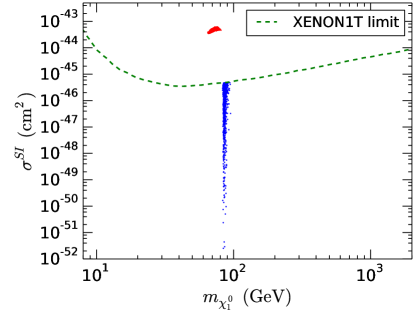
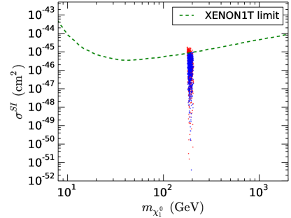
Figure 16: Left: $\chi_{1}^{0}$-neucleon spin-independent cross section as a function of $\chi_{1}^{0}$ mass. 2$\sigma$ upper limit on the cross section from XENON1T experiment has been shown by green dashed line. The blue region corresponds to the MSSM parameter space at 95.6% C.L. for the case shown in Fig. 3 (Case 1a in complete analysis). The red area is corresponds to the 95.6% C.L. region of parameter space for Case 1a in ’fit without direct search’ analysis. Right: same for Case 2b.

The candidatures of the remaining benchmarks are distinctly worse. All these observations indicate that the MSSM, with the lightest neutralino as the only source of cold dark matter in our universe, is a rather unsatisfactory explanation of the observed $\gamma$-ray data from outer space. This conclusion can change if (a) future observations lead to drastic revision of the data used by us, including shapes of distributions, or (b) a robust alternate explanation, possibly based on undetected astrophysical sources, is found for the extra-terrestrial data sets, or (c) much better fits for the MSSM emerge from observation of numerous other stellar objects, compared to which the presently used data get ‘weighted out’.

7 Summary and conclusions

We have analysed extra-terrestrial $\gamma$-ray data with special emphasis on the excess flux within a specific ROI around the GC, which corresponds to $2\degree<|b|<20\degree$ and $|l|<20\degree$, $b$ and $l$ being the galactic latitude and longitude. The excess, mostly in the energy band 1 - 10 GeV, is fitted for four representative kinds of MSSM spectrum. The constraints from all low-energy and collider data are used, along with the limits from direct DM search experiments. Consistency with observations of Reticulum II and M31 is also maintained in the analysis. We also apply the requirement that the lower limit (modulo theoretical uncertainties) on the relic density be satisfied by MSSM contributions, since otherwise the minimality of the model is lost. It is found that the best fit to the data is offered by a scenario with $|M_{1}|$ constrained around 100 GeV, $\mu$ in the range 110 - 125 GeV and $\tan\beta$ = 20 and $m_{A}$ in the range 450 - 550 GeV. A light stop scenario corresponding to $\tan\beta$ = 50 emerges as the second best candidate, where the lighter stop mass is close to 300 GeV and the $\chi^{0}_{1}$ is around 180 GeV. The lower limit on the relic density has a significant role in curving out $2\sigma$ regions in the above parameter regions.

However, if the fits are carried out blindly to direct search constraint, then the $2\sigma$ regions thus obtained are completely gone, indicating that the region presented after the ‘complete fit’ is not even a part of the original outcome of an impartial analysis of the GC $\gamma$-ray data. The situation is not so contradictory for the light stop region, but it corresponds to a distinctly worse fit that the first case, as is reflected by $\chi^{2}_{min}$ and the $p$-values for the two cases. Drawing a parallel with somewhat similar situations in the search for the Higgs boson in the standard electroweak model, the MSSM is found to offer a somewhat unsatisfactory fit for GC $\gamma$-rays, unlike the standard model which fits Higgs-related data rather well.

Before we end, let us re-emphasize an important point that has been already mentioned, namely, that galactic centre excess can be due to other astrophysical sources such as millisecond pulsars (MSPs). This, we re-iterate, is still an open issue. While one may try to interpret the available evidences either in terms of DM annihilation as a possible explanation or perhaps in terms of astrophysical objects like MSPs, we show that the most common and economical DM explanation, namely, that in terms of the MSSM, is fraught with difficulties. It should also be noted that not allowing under-abundance is but one component of this demonstration, a crucial component being the shape of the GC spectrum itself. This becomes obvious when one looks at Table 4 where the statistical significance for the best MSSM scenario even without the relic density lower bound constraint is displayed. Even if under-abundance is allowed, the relative statistical insignificance of the MSSM explanation, as compared with the explanation of the Higgs data in terms of the standard electroweak theory, is something to take serious note of. Such unsatisfactory $p$-values as have been obtained by us are again due to the difficulty in matching the shape, while ensuring consistency with laboratory constraints on the MSSM, and the inescapable dynamics of the spectra that survive such constraints.

Acknowledgements:
We thank Anirban Biswas, Utpal Chattopadhyay, Raj Gandhi, Subhadeep Mondal, Niladri Paul and Tim Tait for helpful comments. The work of AK and BM was partially supported by funding available from the Department of Atomic Energy, Government of India, for the Regional Centre for Accelerator-based Particle Physics (RECAPP), Harish-Chandra Research Institute. TRC acknowledges the hospitality of RECAPP while the project was being formulated, while AK and BM thank the National Centre for Radio Astrophysics, Pune, for hospitality while work was in progress.

References

- [1] J. L. Feng, “Dark Matter Candidates from Particle Physics and Methods of Detection,” Ann. Rev. Astron. Astrophys. 48, 495 (2010) [arXiv:1003.0904 [astro-ph.CO]].
- [2] E. Aprile et al. [XENON Collaboration], “First Dark Matter Search Results from the XENON1T Experiment,” Phys. Rev. Lett. 119, 181301 (2017) [arXiv:1705.06655 [astro-ph.CO]].
- [3] D. S. Akerib et al.. [LUX Collaboration], “Limits on Spin-Dependent WIMP-Nucleon Cross Section Obtained from the Complete LUX Exposure,” Phys. Rev. Lett. 118, 251302, 2017
- [4] D. S. Akerib et al. [LUX Collaboration], “Improved Limits on Scattering of Weakly Interacting Massive Particles from Reanalysis of 2013 LUX Data,” Phys. Rev. Lett. 116, 161301 (2016) [arXiv:1512.03506 [astro-ph.CO]].
- [5] D. S. Akerib et al. [LUX Collaboration], “Results on the Spin-Dependent Scattering of Weakly Interacting Massive Particles on Nucleons from the Run 3 Data of the LUX Experiment,” Phys. Rev. Lett. 116, 161302 (2016) [arXiv:1602.03489 [hep-ex]].
- [6] S. Colafrancesco, S. Profumo and P. Ullio, “Multi-frequency analysis of neutralino dark matter annihilations in the Coma cluster,” Astron. Astrophys. 455, 21 (2006) [astro-ph/0507575].
- [7] M. H. Chan, “Constraining annihilating dark matter by x-ray data,” Astrophys. Space Sci. 362, 147 (2017) [arXiv:1707.00388 [astro-ph.HE]].
- [8] G. Beck and S. Colafrancesco, “A Multi-frequency analysis of dark matter annihilation interpretations of recent anti-particle and -ray excesses in cosmic structures,” JCAP 1605, 013 (2016) [arXiv:1508.01386 [astro-ph.CO]].
- [9] P. A. R. Ade et al. [Planck Collaboration], “Planck 2015 results. XIII. Cosmological parameters,” Astron. Astrophys. 594, A13 (2016) [arXiv:1502.01589 [astro-ph.CO]].
- [10] J. Harz, B. Herrmann, M. Klasen, K. Kovarik and P. Steppeler, “Theoretical uncertainty of the supersymmetric dark matter relic density from scheme and scale variations,” Phys. Rev. D 93, 114023 (2016) [arXiv:1602.08103 [hep-ph]].
- [11] M. Klasen, K. Kovarik and P. Steppeler, “SUSY-QCD corrections for direct detection of neutralino dark matter and correlations with relic density,” Phys. Rev. D 94, 095002 (2016) [arXiv:1607.06396 [hep-ph]].
- [12] M. Badziak, M. Olechowski and P. Szczerbiak, “Spin-dependent constraints on blind spots for thermal singlino-higgsino dark matter with(out) light singlets,” JHEP 1707, 050 (2017) [arXiv:1705.00227 [hep-ph]].
- [13] A. Achterberg, M. van Beekveld, S. Caron, G. A. Gómez-Vargas, L. Hendriks and R. Ruiz de Austri, “Implications of the Fermi-LAT Pass 8 Galactic Center Excess on Supersymmetric Dark Matter,” arXiv:1709.10429 [hep-ph].
- [14] A. Achterberg, S. Amoroso, S. Caron, L. Hendriks, R. Ruiz de Austri and C. Weniger, “A description of the Galactic Center excess in the Minimal Supersymmetric Standard Model,” JCAP 1508, 006 (2015) [arXiv:1502.05703 [hep-ph]].
- [15] G. Bertone, F. Calore, S. Caron, R. Ruiz, J. S. Kim, R. Trotta and C. Weniger, “Global analysis of the pMSSM in light of the Fermi GeV excess: prospects for the LHC Run-II and astroparticle experiments,” JCAP 1604, 037 (2016) [arXiv:1507.07008 [hep-ph]].
- [16] F. Calore, I. Cholis, C. McCabe and C. Weniger, “A Tale of Tails: Dark Matter Interpretations of the Fermi GeV Excess in Light of Background Model Systematics,” Phys. Rev. D 91, 063003 (2015) [arXiv:1411.4647 [hep-ph]].
- [17] A. Butter, S. Murgia, T. Plehn and T. M. P. Tait, “Saving the MSSM from the Galactic Center Excess,” Phys. Rev. D 96, 035036 (2017) [arXiv:1612.07115 [hep-ph]].
- [18] S. Profumo, “An Introduction to Particle Dark Matter”, Published by World Scientific Publishing Europe Ltd.(2017)
- [19] M. Ajello et al. [Fermi-LAT Collaboration], “Fermi-LAT Observations of High-Energy -Ray Emission Toward the Galactic Center,” Astrophys. J. 819, 44 (2016) [arXiv:1511.02938 [astro-ph.HE]].
- [20] F. Calore, I. Cholis and C. Weniger, “Background Model Systematics for the Fermi GeV Excess,” JCAP 1503, 038 (2015) [arXiv:1409.0042 [astro-ph.CO]].
- [21] M. Ackermann et al. [Fermi-LAT Collaboration], “The Fermi Galactic Center GeV Excess and Implications for Dark Matter,” Astrophys. J. 840, 43 (2017) [arXiv:1704.03910 [astro-ph.HE]].
- [22] C. Karwin, S. Murgia, T. M. P. Tait, T. A. Porter and P. Tanedo, “Dark Matter Interpretation of the Fermi-LAT Observation Toward the Galactic Center,” Phys. Rev. D 95, 103005 (2017) [arXiv:1612.05687 [hep-ph]].
- [23] M. Thierbach, U. Klein and R. Wielebinski, “The diffuse radio emission from the coma cluster at 2.675 ghz and 4.85 ghz,” Astron. Astrophys. 397, 53 (2003) [astro-ph/0210147].
- [24] A. Geringer-Sameth, M. G. Walker, S. M. Koushiappas, S. E. Koposov, V. Belokurov, G. Torrealba and N. W. Evans, “Indication of Gamma-ray Emission from the Newly Discovered Dwarf Galaxy Reticulum II,” Phys. Rev. Lett. 115, 081101 (2015) [arXiv:1503.02320 [astro-ph.HE]].
- [25] Y. Zhao, X. J. Bi, P. F. Yin and X. M. Zhang, “Searching for Gamma-Ray Emission from Reticulum II by Fermi-LAT,” arXiv:1702.05266 [astro-ph.HE].
- [26] A. Drlica-Wagner et al. [Fermi-LAT and DES Collaborations], “Search for Gamma-Ray Emission from DES Dwarf Spheroidal Galaxy Candidates with Fermi-LAT Data,” Astrophys. J. 809, L4 (2015) [arXiv:1503.02632 [astro-ph.HE]].
- [27] M. Ackermann et al. [Fermi-LAT Collaboration], “Dark matter constraints from observations of 25 Milky Way satellite galaxies with the Fermi Large Area Telescope,” Phys. Rev. D 89, 042001 (2014) [arXiv:1310.0828 [astro-ph.HE]].
- [28] R. D. Griffin, X. Dai and C. S. Kochanek, “New Limits On Gamma-Ray Emission From Galaxy Clusters,” Astrophys. J. 795, L21 (2014) [arXiv:1405.7047 [astro-ph.HE]].
- [29] K. N. Abazajian and M. Kaplinghat, “Detection of a Gamma-Ray Source in the Galactic Center Consistent with Extended Emission from Dark Matter Annihilation and Concentrated Astrophysical Emission,” Phys. Rev. D 86, 083511 (2012) Erratum: [Phys. Rev. D 87, 129902 (2013)] [arXiv:1207.6047 [astro-ph.HE]].
- [30] Q. Yuan and B. Zhang, “Millisecond pulsar interpretation of the Galactic center gamma-ray excess,” JHEAp 3-4, 1 (2014) [arXiv:1404.2318 [astro-ph.HE]].
- [31] N. Mirabal, “Dark matter vs. Pulsars: Catching the impostor,” Mon. Not. Roy. Astron. Soc. 436, 2461 (2013) [arXiv:1309.3428 [astro-ph.HE]].
- [32] R. Bartels, S. Krishnamurthy and C. Weniger, “Strong support for the millisecond pulsar origin of the Galactic center GeV excess,” Phys. Rev. Lett. 116, 051102 (2016) [arXiv:1506.05104 [astro-ph.HE]].
- [33] H. Ploeg, C. Gordon, R. Crocker and O. Macias, “Consistency Between the Luminosity Function of Resolved Millisecond Pulsars and the Galactic Center Excess,” JCAP 1708, 015 (2017) [arXiv:1705.00806 [astro-ph.HE]].
- [34] J. Petrović, P. D. Serpico and G. Zaharijaš, “Galactic Center gamma-ray ”excess” from an active past of the Galactic Centre?,” JCAP 1410, 052 (2014) [arXiv:1405.7928 [astro-ph.HE]].
- [35] E. Carlson and S. Profumo, “Cosmic Ray Protons in the Inner Galaxy and the Galactic Center Gamma-Ray Excess,” Phys. Rev. D 90, 023015 (2014) [arXiv:1405.7685 [astro-ph.HE]].
- [36] K. N. Abazajian, “The Consistency of Fermi-LAT Observations of the Galactic Center with a Millisecond Pulsar Population in the Central Stellar Cluster,” JCAP 1103, 010 (2011) [arXiv:1011.4275 [astro-ph.HE]].
- [37] G. Ponti, M. R. Morris, R. Terrier, A. Goldwurm “Traces of past activity in the Galactic Centre,” [arXiv:1210.3034]
- [38] I. Cholis, D. Hooper and T. Linden, “Challenges in Explaining the Galactic Center Gamma-Ray Excess with Millisecond Pulsars,” JCAP 1506, 043 (2015) [arXiv:1407.5625 [astro-ph.HE]].
- [39] T. Linden, “Known Radio Pulsars Do Not Contribute to the Galactic Center Gamma-Ray Excess,” Phys. Rev. D 93, 063003 (2016) [arXiv:1509.02928 [astro-ph.HE]].
- [40] T. Daylan, D. P. Finkbeiner, D. Hooper, T. Linden, S. K. N. Portillo, N. L. Rodd and T. R. Slatyer, “The characterization of the gamma-ray signal from the central Milky Way: A case for annihilating dark matter,” Phys. Dark Univ. 12, 1 (2016) [arXiv:1402.6703 [astro-ph.HE]].
- [41] X. Huang, T. Enßlin and M. Selig, “Galactic dark matter search via phenomenological astrophysics modeling,” JCAP 1604, 030 (2016) [arXiv:1511.02621 [astro-ph.HE]].
- [42] A. Achterberg, M. van Beekveld, W. Beenakker, S. Caron and L. Hendriks, “Comparing Galactic Center MSSM dark matter solutions to the Reticulum II gamma-ray data,” JCAP 1512, 013 (2015) [arXiv:1507.04644 [hep-ph]].
- [43] G. Beck and S. Colafrancesco, “A Multi-frequency analysis of possible Dark Matter Contributions to M31 Gamma-Ray Emissions,” JCAP 1710, 007 (2017) [arXiv:1707.09787 [astro-ph.CO]].
- [44] M. Ackermann et al. [Fermi-LAT Collaboration], “Observations of M31 and M33 with the Fermi Large Area Telescope: A Galactic Center Excess in Andromeda?,” Astrophys. J. 836, 208 (2017) [arXiv:1702.08602 [astro-ph.HE]].
- [45] A. Kar, S. Mitra, B. Mukhopadhyaya and T. R. Choudhury, “Do astrophysical data disfavour the minimal supersymmetric standard model?,” arXiv:1711.09069 [hep-ph].
- [46] M. Baak, M. Goebel, J. Haller, A. Hoecker, D. Ludwig, K. Moenig, M. Schott and J. Stelzer, “Updated Status of the Global Electroweak Fit and Constraints on New Physics,” Eur. Phys. J. C 72, 2003 (2012) [arXiv:1107.0975 [hep-ph]].
- [47] H. Flacher, M. Goebel, J. Haller, A. Hocker, K. Monig and J. Stelzer, “Revisiting the Global Electroweak Fit of the Standard Model and Beyond with Gfitter,” Eur. Phys. J. C 60, 543 (2009) Erratum: [Eur. Phys. J. C 71, 1718 (2011)] [arXiv:0811.0009 [hep-ph]].
- [48] P. Agrawal, B. Batell, P. J. Fox and R. Harnik, “WIMPs at the Galactic Center,” JCAP 1505, 011 (2015) [arXiv:1411.2592 [hep-ph]].
- [49] M. Cirelli et al., “PPPC 4 DM ID: A Poor Particle Physicist Cookbook for Dark Matter Indirect Detection,” JCAP 1103, 051 (2011) Erratum: [JCAP 1210, E01 (2012)] [arXiv:1012.4515 [hep-ph]].
- [50] F. Iocco, M. Pato, G. Bertone and P. Jetzer, “Dark Matter distribution in the Milky Way: microlensing and dynamical constraints,” JCAP 1111, 029 (2011) [arXiv:1107.5810 [astro-ph.GA]].
- [51] R. Catena and P. Ullio, “A novel determination of the local dark matter density,” JCAP 1008, 004 (2010) [arXiv:0907.0018 [astro-ph.CO]].
- [52] P. Salucci, F. Nesti, G. Gentile and C. F. Martins, “The dark matter density at the Sun’s location,” Astron. Astrophys. 523, A83 (2010) [arXiv:1003.3101 [astro-ph.GA]].
- [53] www.ru.nl/publish/pages/760763/verslag.pdf
- [54] Bonnivard, V. et al., “Dark matter annihilation and decay profiles for the Reticulum II dwarf spheroidal galaxy,” 2015, ApJ, 808, L36
- [55]
- [56] A. Djouadi, J. L. Kneur and G. Moultaka, “SuSpect: A Fortran code for the supersymmetric and Higgs particle spectrum in the MSSM,” Comput. Phys. Commun. 176, 426 (2007) [hep-ph/0211331].
- [57] G. Aad et al. [ATLAS Collaboration], “Measurement of the Higgs boson mass from the and channels with the ATLAS detector using 25 fb-1 of collision data,” Phys. Rev. D 90, 052004 (2014) [arXiv:1406.3827 [hep-ex]].
- [58] V. Khachatryan et al. [CMS Collaboration], “Precise determination of the mass of the Higgs boson and tests of compatibility of its couplings with the standard model predictions using proton collisions at 7 and 8 TeV,” Eur. Phys. J. C 75, 212 (2015) [arXiv:1412.8662 [hep-ex]].
- [59] B. C. Allanach, A. Djouadi, J. L. Kneur, W. Porod and P. Slavich, “Precise determination of the neutral Higgs boson masses in the MSSM,” JHEP 0409, 044 (2004) [hep-ph/0406166].
- [60] C. Patrignani et al. (Particle Data Group), Chin. Phys. C, 40, 100001 (2016) and 2017 update
- [61] A. Lipniacka, “Understanding SUSY limits from LEP,” hep-ph/0210356.
- [62] G. Aad et al. [ATLAS Collaboration], “Search for the electroweak production of supersymmetric particles in collisions with the ATLAS detector,” Phys. Rev. D 93, 052002
- [63] LEPSUSYWG, ALEPH, DELPHI, L3 and OPAL experiments, note LEPSUSYWG/yy-nn (http://lepsusy.web.cern.ch/lepsusy/Welcome.html).
- [64] M. Aaboud et al. [ATLAS Collaboration], “Search for Supersymmetry in final states with missing transverse momentum and multiple -jets in proton–proton collisions at TeV with the ATLAS detector,” arXiv:1711.01901 [hep-ex].
- [65] A. M. Sirunyan et al. [CMS Collaboration], “Search for supersymmetry in multijet events with missing transverse momentum in proton-proton collisions at 13 TeV,” Phys. Rev. D 96, 032003 (2017) [arXiv:1704.07781 [hep-ex]].
- [66] M. Aaboud et al. [ATLAS Collaboration], “Search for squarks and gluinos in events with an isolated lepton, jets and missing transverse momentum at = 13 TeV with the ATLAS detector,” arXiv:1708.08232 [hep-ex].
- [67] A. M. Sirunyan et al. [CMS Collaboration], “Search for new phenomena with the variable in the all-hadronic final state produced in proton–proton collisions at TeV,” Eur. Phys. J. C 77, 710 (2017) [arXiv:1705.04650 [hep-ex]].
- [68] M. Aaboud et al. [ATLAS Collaboration], “Search for a scalar partner of the top quark in the jets plus missing transverse momentum final state at =13 TeV with the ATLAS detector,” arXiv:1709.04183 [hep-ex].
- [69] M. Aaboud et al. [ATLAS Collaboration], “Search for direct top squark pair production in final states with two leptons in TeV collisions with the ATLAS detector,” arXiv:1708.03247 [hep-ex].
- [70] A. M. Sirunyan et al. [CMS Collaboration], “Search for the pair production of third-generation squarks with two-body decays to a bottom or charm quark and a neutralino in proton-proton collisions at sqrt(s) = 13 TeV,” arXiv:1707.07274 [hep-ex].
- [71] https://lapth.cnrs.fr/micromegas/v4.1/manual4.1.pdf
- [72] G. Belanger, F. Boudjema, A. Pukhov and A. Semenov, “MicrOMEGAs: A Program for calculating the relic density in the MSSM,” Comput. Phys. Commun. 149, 103 (2002) [hep-ph/0112278].
- [73] G. Aad et al. [ATLAS Collaboration], “Summary of the ATLAS experiment’s sensitivity to supersymmetry after LHC Run 1 — interpreted in the phenomenological MSSM,” JHEP 1510, 134 (2015) [arXiv:1508.06608 [hep-ex]].
- [74] The ATLAS collaboration [ATLAS Collaboration], “Search for electroweak production of supersymmetric particles in the two and three lepton final state at TeV with the ATLAS detector,” ATLAS-CONF-2017-039.
- [75] M. Aaboud et al. [ATLAS Collaboration], “Search for Minimal Supersymmetric Standard Model Higgs bosons and for a boson in the final state produced in collisions at TeV with the ATLAS Detector,” Eur. Phys. J. C 76, 585 (2016) [arXiv:1608.00890 [hep-ex]].
- [76] M. Aaboud et al. [ATLAS Collaboration], “Search for additional heavy neutral Higgs and gauge bosons in the ditau final state produced in 36 fb-1 of collisions at = 13 TeV with the ATLAS detector,” arXiv:1709.07242 [hep-ex].
- [77] Daniel Foreman-Mackey et al., “emcee: The MCMC Hammer,” arXiv:1202.3665 [astro-ph.IM]
- [78] T. Sjostrand, S. Mrenna and P. Z. Skands, “PYTHIA 6.4 Physics and Manual,” JHEP 0605, 026 (2006) [hep-ph/0603175].
- [79] Nuclear Physics B, Part. Phys., Vol. 360, No. 1, p. 145 - 179
- [80] E. Storm, T. E. Jeltema, M. Splettstoesser and S. Profumo, “Synchrotron Emission from Dark Matter Annihilation: Predictions for Constraints from Non-detections of Galaxy Clusters with New Radio Surveys,” Astrophys. J. 839, 33 (2017) [arXiv:1607.01049 [astro-ph.CO]].
- [81] M. J. Hardcastle, “Synchrotron and inverse-Compton emission from radio galaxies with non-uniform magnetic field and electron distributions,” Mon. Not. Roy. Astron. Soc. 433, 3364 (2013) [arXiv:1306.1640 [astro-ph.HE]].
- [82] A. Natarajan, J. E. Aguirre, K. Spekkens and B. S. Mason, “Green Bank Telescope Constraints on Dark Matter Annihilation in Segue I,” arXiv:1507.03589 [astro-ph.CO].
- [83] Longair, M. 1994, ’High Energy Astrophysics’, vol. 2, Cambridge University Press
- [84] J. F. Navarro, C. S. Frenk and S. D. M. White, Astrophys. J. 462, 563 (1996) [astro-ph/9508025].
- [85] Bonafede, A., et al., “The Coma cluster magnetic field from Faraday rotation measures,” 2010, AA, 513, A30, arXiv:1002.0594 [astro-ph.CO]