Lattice Boltzmann Benchmark Kernels as a Testbed for Performance Analysis

Abstract

Lattice Boltzmann methods (LBM) are an important part of current computational fluid dynamics (CFD). They allow easy implementations and boundary handling. However, competitive time to solution not only depends on the choice of a reasonable method, but also on an efficient implementation on modern hardware. Hence, performance optimization has a long history in the lattice Boltzmann community. A variety of options exists regarding the implementation with direct impact on the solver performance. Experimenting and evaluating each option often is hard as the kernel itself is typically embedded in a larger code base. With our suite of lattice Boltzmann kernels we provide the infrastructure for such endeavors. Already included are several kernels ranging from simple to fully optimized implementations. Although these kernels are not fully functional CFD solvers, they are equipped with a solid verification method. The kernels may act as an reference for performance comparisons and as a blue print for optimization strategies. In this paper we give an overview of already available kernels, establish a performance model for each kernel, and show a comparison of implementations and recent architectures.

1 Introduction

Lattice Boltzmann methods are used in various fields to simulate fluid flows. Besides different discretizations and collision models a lot of choices arise concerning data layout, lattice representation, addressing, and propagation step implementations. Furthermore, depending on the chosen combination of these options, several hardware and software optimizations may or may not be possible. The interaction between all these components can have a severe impact on the resulting performance. Experimenting with all these options is often hard as the solvers are embedded in larger code bases where it is often not possible to easily change the implementation. With the lattice Boltzmann benchmark kernels we try to create a framework for an easy evaluation of different data layouts, addressing schemes, propagation steps, and optimizations. Furthermore, we deliver several reference implementations of kernels in C which range from standard unoptimized to highly optimized versions. The suite is GPLv3 licensed and publicly available.

The paper is outlined as follows. In Sect. 2 we give a short overview of the LBM model used, supported architectures, and included sample geometries. Furthermore, the verification scheme used to validate implementations for their correctness is presented as well as important points considered regarding benchmarking. The available implementations, including the different options regarding data layout, addressing, etc., are discussed in Sect. 3. In Sect. 4 we establish a performance model and evaluate the implementations’ performance on one selected architecture. Exemplarily, we discuss several performance effects on this system. A comparison of the implementation across several current hardware architectures is presented in Sect. 5. Finally Sect. 6 summarizes the article and gives an outlook on planned work.

2 Benchmark Suite

Throughout the suite, all benchmark kernels use a D3Q19 discretication with the two-relaxation-time (TRT) collision model [8]. Depending on the kernel, half or full way bounce back [11] is used. PDFs are always stored as double precision floating point numbers.

The suite is implemented in C99 and currently focus on the x86-64 platform. Configurations for recent Linux and GCC/Intel compilers are available. Some highly optimized kernels use explicit SSE/AVX intrinsics. Although we do not include intrinsics for AVX2 or FMA (fused multiply add), we observed that the Intel compiler transforms AVX intrinsics into these ISA extensions.

As already noted, the focus of this contribution is clearly on performance studies and optimizations. The suite does not provide a fully-featured flow solver. This allows us to keep the code modular and easily extensible as we are planning to provide further kernels as for now only highly optimized “list”-based kernels are included (see Sect. 3).

For evaluating the performance with respect to the structure of the simulation domain, we include several synthetic geometries. Simple homogeneous arbitrarily scalable geometries like channel or pipe which represent an empty channel with rectangular or a staircase approximation of a circular cross section, respectively. Furthermore, blocks is a heterogeneous geometry where equidistant blocks of obstacles are distributed over the domain with adjustable dimensions and distance of the blocks to each other. The first two geometries can be used to benchmark best-cases as they are homogeneous and nearly no bounce-back will occur. The blocks geometry on the other side can be used to study the impact on performance when the amount of bounce-back is increased and – depending on the kernel – vectorized updates of fluid nodes are no longer completely possible.

2.1 Verification

In order to check if computations performed by a benchmark kernel are correct, the framework has an inbuilt verification setup. For performance reasons this must explicitly be turned on during compilation as the runtime increases significantly.

For verification a Poision flow is simulated and compared to the analytical solution. As in [18], therefore a geometry with periodic boundaries in x and y direction is setup, i. e. fluid between two slabs, and on each fluid node a constant body force is applied. After enough iterations, the fluid field in z direction (between the two slabs) should exhibit a parabola profile and is compared to the analytical solution.

2.2 Benchmarking

As benchmarking is a non-trivial endeavor, we try to cover as many problematic setups as possible already in the implementation:

Thread Affinity

We support direct pinning (setting the affinity) of threads by the user. This binds a thread to the specified core and avoids the thread being migrated to different cores by the OS.

NUMA placement

Linux uses by default a first-touch placement strategy. This means that a memory page is placed into the NUMA locality domain of the core first touching it. The initialization of the lattice and important accompanying structures respect this principle by using the same parallelization as the main compute loop later on, but correct pinning by the user is required.

Huge Pages

Current Linux kernels support transparent huge pages. This means that memory allocated with small $4$ KiB pages is replaced with larger pages (typically $2$ MiB). In our case, this is in general beneficial as less TLB misses and page walks occur. For this to work, the corresponding OS setting must be enabled to perform this task every time or on request. The latter requires an additional call to madvise(MADV_HUGEPAGE) after memory allocation. We perform this for lattice and adjacency list allocation.

Uncovered Points

Several settings are out of the control of the benchmark kernels themselves, and the user must take care of these, like fixing the CPU frequency, compiling for the correct architecture, eventually override the CPU dispatcher, or observe no other tasks are running, to name just a few.

3 Implemented Kernels

kernel	prop.	data	addr.	parallel	loop	padding	$B_{l}$	micro-
name	step	layout			blocking		[B/FLUP]	benchmark
(blk-)push-soa	OS	SoA	D	x	(x)–	–	456	copy-19
(blk-)push-aos	OS	AoS	D	x	(x)–	–	456	copy-19
(blk-)pull-soa	OS	SoA	D	x	(x)–	–	456	copy-19
(blk-)pull-aos	OS	AoS	D	x	(x)–	–	456	copy-19
aa-soa	AA	SoA	D	x	x	–	304	update-19
aa-aos	AA	AoS	D	x	x	–	304	update-19
aa-vec-soa	AA	SoA	D	x	x	–	304	update-19
list-push-soa	OS	SoA	I	x	x	x	528	copy-19
list-push-aos	OS	AoS	I	x	x	–	528	copy-19
list-pull-soa	OS	SoA	I	x	x	x	528	copy-19
list-pull-aos	OS	AoS	I	x	x	–	528	copy-19
list-pull-split-nt-1s-soa	OS	SoA	I	x	x	x	376	copy-19-nt-sl
list-pull-split-nt-2s-soa	OS	SoA	I	x	x	x	376	copy-19-nt-sl
list-aa-soa	AA	SoA	I	x	x	x	340	update-19
list-aa-aos	AA	AoS	I	x	x	–	340	update-19
list-aa-ria-soa	AA	SoA	I	x	x	x	304–342	update-19
list-aa-pv-soa	AA	SoA	I	x	x	x	304–342	update-19

Table 1: Implemented kernels with their respective features. Propagation step OS denotes one step. The addressing scheme (addr.) is direct (D) for a full array approach or indirect (I) for a list approach. The loop balance $B_{l}$ is based on a D3Q19 discretization, double precision floating point numbers for PDFs and $4$ b integers for elements of the adjacency list in case of a list approach.

For implementing a LBM kernel various options regarding lattice representation, data layout, or propagation step exist. In the following we give a short overview of the most common approaches which we implemented in the benchmark kernels. For more details refer to [29, 9, 35, 33, 34, 31]. All features of the implemented kernels are summarized in Table 1.

Lattice Representation

The first option describes how the PDFs of the simulation domain should be represented. With the marker and cell approach  [12] a full multi-dimensional array, holding fluid and obstacle nodes, is used together with a flag field for distinguishing the node types. PDFs can be accessed by direct addressing, i. e. by simple index arithmetic. Especially in porous media like geometries, it is beneficial to store only the fluid nodes. These can be arranged in an 1-D vector accompanied by an adjacency list [24, 18, 35, 2, 26, 27, 13]. Here, each node’s neighbors are accessed via indirect addressing, as it requires a lookup in the adjacency list. In this work we use the terms “full array” and “list” for the two representations, respectively. Not covered here are patch-based approaches as used in [7, 6] or semi-direct addressing which merges the full array and list approach as described in [15].

Data Layout

The data layout can be chosen independently of the lattice representation. It describes in which order PDFs of the nodes are contiguously stored in memory. We concentrate on two incarnations: array-of-structures (AoS) and structure-of-arrays (SoA). Sometimes the terms collision optimized layout and propagation optimized layout are used [29], respectively. In the first approach, the PDFs of a node are stored consecutive in memory whereas in the latter approach PDFs of one direction are consecutive. Hybrid forms such as AoSoA or SoAoS exist, but are not covered here.

One Step Kernels

The collision step is defined by the chosen collision model, like SRT [3, 21], TRT [8], or MRT [4], but the propagation step provides options for optimizations. Typically, collision and propagation are fused into one step and two lattices are utilized: one source and one destination lattice. This kind of implementation is called one step [20] and can be implemented in two flavors: push and pull. With push, the PDFs of a node are read from the source lattice, collided, and propagated to the neighbor nodes in the destination lattice. In the case of pull, propagation is performed first, by reading PDFs from the neighbors in the source lattice, colliding them and then writing them to the local node in the destination lattice. One step can be combined with all discussed domain representations and data layouts. The corresponding implementations without optimizations are called (list-)push/pull-aos/soa in the suite.

One Step Kernels with Non-Temporal Stores

Optimizations regarding one step include avoiding the write allocate for stores [29]. Before a normal store is executed, data residing at the specific location is first loaded into the cache before being modified. This is called write allocate. As the written data is not reused until the next time step (and the lattice is so large that the data in cache will already have been evicted), non-temporal stores can be used which avoid the extra read operation and thus save memory bandwidth. In order to work efficiently, it is best to write in a granularity of complete cache lines which on all considered architectures are $64$ b long. Furthermore, the highest bandwidth with this kind of stores typically allows one or two concurrent non-temporal store streams only. We implement this by strip mining the update process to a certain number of nodes which are loaded, collided, and finally written back to memory with one or two store streams [5, 35]. We implemented this only for the list representation lattice with SoA data layout and OS pull, as here stores occur naturally consecutive. The kernels implementing these optimizations are list-pull-split-nt-(1s/-s2)-soa.

AA Pattern Kernels

The propagation step AA pattern [1] requires only one lattice and writes only to locations which previously have been read (kernels (list-)aa-soa/-aos). It consists of an even and odd time step. The even time step only requires node local accesses. Even with a list approach it does not require an indirect access and is easily (manually) vectorizable with an SoA data layout. The odd time step reads and writes to neighbors, hence, both require the same indirect access with a list. In an optimized version, we introduce a run length coding where the additional lookup can be neglected for consecutive nodes, sharing the same access pattern. This, we call reduced indirect addressing or short RIA [32, 34]. As the run length coding describes nodes which can be loaded and stored contiguously, we use it to implement a partial vectorization (PV) of the odd time step [32, 34]. The latter two optimizations are only implemented for the list version of AA as list-aa-ria-soa and list-aa-pv-soa. In the case of a full array implementation, the even and odd time step can be fully vectorized. This is done in the aa-vec-soa kernel.

Not Considered Propagation Steps

Furthermore propagation steps exist, but are (currently) not part of the suite. An incomplete list includes: i) two-step implementation with split collision and propagation increase the loop balance dramatically, ii) compressed grid [20] utilizes only one lattice, traversing it forward and backwards, iii) Esoteric Twist [14, 23, 19, 22], which requires only one lattice, exhibits with indirect addressing the lowest constant loop balance for D3Q19 with $328$ B/FLUP, and requires only tree neighbors to be stored in the adjacency list [19, 22], or iv) temporal blocking, were several updates to a subdomain are performed before it is written back to memory [20, 28, 10, 17].

3.1 Parallelization

All implemented kernels are OpenMP parallel. In case of the unblocked one step kernels utilizing a full array (push-aos, push-soa, pull-aos, and pull-soa), the loop nest over the three spatial dimensions is parallelized with an OpenMP parallel for collapse(3) clause. In principal this approach would also support loop blocking, but could lead to load imbalances. In order to avoid this for the blocked variants of these kernels (blk-*), a different approach is used. Each thread gets one equally sized part of the domain which is cut in x direction. On each subdoamin, loop blocking is then applied.

For the list based kernels, simply the loop over the fluid nodes is parallelized. Higher optimized kernels like list-pull-split-nt-(1s/-2s)-soa, list-aa-ria-soa, and list-aa-pv-soa require a manual scheduling, e. g. to ensure alignment constraints.

3.2 Bounce-Back and Periodicity Handling

Full array kernels iterate over the full domain and initially do not distinguish between fluid and solid. In a separate step, bounce-back and correct periodicity of the simulation domain is treated. The list kernels allow automatic handling of bounce-back and periodicity via the adjacency list. Hence, they do not need an additional “correction” step.

4 Performance Discussion

name		BDW-S
processor		Intel Xeon
name		E5-2630 v4
micro.		Broadwell
freq	[GHz]	2.2
cores		10
ISA		AVX2
sockets		2
L1 cache	[KiB]	32
L2 cache	[KiB]	256
L3 cache	[MiB]	25
socket bandwidth
copy	[GB/s]	53.9
copy-19	[GB/s]	48.0
copy-19-nt-sl	[GB/s]	48.2
update-19	[GB/s]	51.1

Table 2: Specifications of the BDW-S system. Bandwidths for copy and copy-19 include write allocate. For copy-19-nt-sl non-temporal stores are used.

For discussing the achieved performance of the kernels we firstly introduce the Roofline performance model. Afterwards, we present the scaling behaviour of the kernels’ performance on one socket of the BDW-S system described in Table 2. Furthermore, we discuss the impact of loop blocking, padding, and heterogeneous geometries. Hereby we limit us to the list based AA pattern kernels. For all benchmarks in this and the next Sect. we fixed the frequency of the processor to its nominal frequency and set the affinity of each thread explicitly. We use Intel C Compiler 17.0.1 and compile with AVX2 and FMA support enabled.

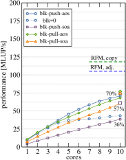
(a) full array, OS

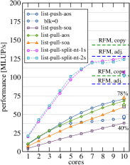
(b) list, OS

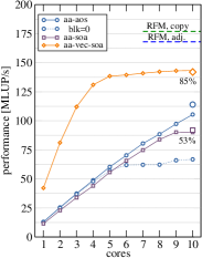
(c) full array, AA

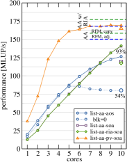
(d) list, AA

Figure 1: Performance of kernels on BDW-S system depending on the number of cores. Single symbols show performance value obtained when SMT was active and all SMT cores of a socket are used. Roofline model predictions are given with two different memory bandwidths as input: (i) the measured copy bandwidth (RFM, copy) and (ii) the bandwidth measured with the corresponding micro-benchmark for each kernel from Table 1 (RFM, adjusted). Percentage values show the reached Roofline performance for selected curves.

4.1 Performance Model

LBM for a D3Q19 discretization, TRT collision model, and double precision floating point numbers is reckoned to be memory bound. Therefore, we use the loop balance $B_{l}$ as the relevant metric, i. e. the number of bytes that must be transferred between processor and memory for the update of one fluid lattice node in units of B/FLUP. We use this as input for the Roofline model [30] to derive an upper performance limit for each kernel. The loop balance of each kernel is found in Table 1 and is taken from [33, 34]. Performance $P_{\text{max}}$ in the memory bandwidth limited case is

$$P_{\text{max}}=\frac{B}{B_{l}},$$ (1)

where $B$ denotes the achievable memory bandwidth. How much bandwidth is attainable depends heavily on the access pattern. We use for a general prediction the STREAM copy [16] bandwidth (copy two arrays, without non-temporal stores, including write-allocate). Furthermore, we use three adjusted micro-benchmarks which resemble the nature of the kernels more specifically:

• copy-19: concurrently copies 19 arrays (19 read and 19 write streams),

• copy-19-nt-sl: concurrently copies 19 arrays with strip mining and using only one concurrent non-temporal store stream for write back, and

• update-19: updates concurrently 19 arrays.

Which micro-benchmark is used for which kernel is found in Table 1. Table 3 reports the measured bandwidths of all evaluated systems.

4.2 Socket Scaling

Figure 1 shows strong scaling of the implemented kernels’ performance depending on the number of cores on one socket of the BDW-S system from Table 2. As geometry channel with dimensions of $500\times 100\times 100$ nodes is used. For using the full socket, the green and blue dashed lines show the Roofline model predictions for each kernel when the memory bandwidth achieved with copy or the corresponding micro-benchmark of a kernel (see Table 1) is used, respectively. For kernels with AoS data layout performance of several blocking factors is measured, but only the best performance is reported.

The unoptimized one step kernels in Fig. 1a with a full array lattice representation reach a low fraction of the predicted Roofline model performance, indicated as percentage value for selected kernels in the graph. Especially blk-push-soa reaches only $36$ %. By manually padding the array we could lift the performance to $72$ MFLUP/s. Measuring the data traffic with likwid [25] for the bad case shows a $6$ % increased loop balance throughout the memory hierarchy. With array padding the measured loop balance between L1/L2 cache is increased by over $400$ % and between L3 cache/memory by about $26$ %. The fraction of L1/L2 TLB misses is in both cases nearly equal. This indicates that the initially poor performance was not caused by TLB or cache thrashing and requires further investigation. The AoS based kernels require a loop blocking which is discussed in more detail in the next Sect. 4.3. However, for blk-push-aos we exemplarily show the effect. The dotted lines in Fig. 1a–d show the performance without this technique applied, which causes a drop by nearly $60$ % in performance. In general if the lower performance of the kernels would be caused by under-utilization of core resources, e. g. introduced through pipeline bubbles, using SMT threads could help. Single large symbols indicate the usage of the $20$ virtual cores on BDW-S in Fig. 1. Only blk-push-soa’s performance is improved, but below the value we reached by manual array padding.

The list based kernels in Fig. 1b show nearly the same behavior, including the low performance of list-push-soa. At most $78$ % of the maximum attainable performance is reached. The list based kernels incorporating non-temporal stores list-pull-split-nt-(1s/-2s)-soa in Fig˙1b meet nearly the prediction. Using SMT with these kernels shows a contrary effect, as the performance decreases. This might be caused by too many non-temporal store streams per physical core. For the full array kernels we currently do not implement this optimization, therefore it is not shown.

AA pattern kernels have a significantly lower loop balance compared to the one step implementations, hence, the Roofline model predictions are higher. For AA pattern the characteristics between full array and list in Fig. 1c and 1d are different, respectively. The full array aa-soa reaches only $53$ % of the predicted performance. Additional manual padding did not increase the performance. The aa-aos kernel with loop blocking applied is slightly better and only aa-vec-soa, the manually vectorized kernel, reaches $85$ % of the Roofline performance. Measurements show, the latter one saturates the memory bandwidth, but exhibits a loop balance of $B_{l}=323$ B/FLUP. Why it is $6$ % higher than the theoretical one of $B_{l}=304$ B/FLUP is unclear. Also this effect requires a more detailed analysis. The single core performance of aa-vec-soa starts at a much higher value and saturates early compared to the unoptimized AA pattern kernels. This effect is caused by the vectorized even and odd time step as the (theoretical) loop balance is the same for all AA kernels with full array. Utilizing SMT is on this machine only beneficial for aa-aos. The remaining kernels are unaffected.

List based AA pattern kernels reach a higher performance level. Here, list-aa-soa gains around $90$ % of the prediction and list-aa-aos is only slightly slower. This is interesting as both kernels’ loop balance is $B_{l}=340$ B/FLUP whereas the corresponding full array kernels’ loop balance is $B_{l}=304$ B/FLUP. The list-aa-ria-soa and list-aa-pv-soa kernels have the same loop balance which depends on the geometry. For channel we have $B_{l}=305$ B/FLUP, but only the latter kernel seems to profit from this optimization, although measuring the memory traffic indicates both kernels reach the theoretical loop balance. The list-aa-pv-soa kernel uses, as aa-vec-soa, a vectorized even and partially vectorized odd time step, which causes the single core performance to start at a higher value and in total saturate with less cores. Especially with such an homogeneous domain as channel around $99$ % of the fluid nodes can be updated vectorized in the odd time step. The usage of SMT has no or even a negative impact on the performance.

Please note that the current implementations of all full array kernels iterate over all nodes, whether they are fluid or obstacle. Geometries with a higher fraction of obstacles than channel will cause a performance drop as only the number of updated fluid nodes is relevant.

4.3 Loop Blocking

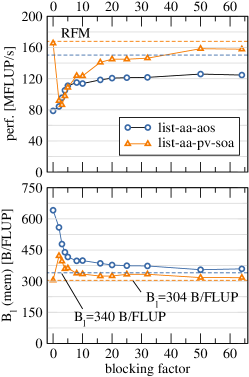
Figure 2: Performance of list-aa-aos and list-aa-pv-soa on ten cores of BDW-S system depending on blocking factor. Benchmark geometry is channel with dimensions of $500\times 100\times 100$ nodes. Blocking factor of zero is equal to no blocking being performed.

It is well known that AoS based kernels require the layer condition to be fulfilled to achieve higher performance [29]. In the case of channel with dimensions of $500\times 100\times 100$ nodes one layer is one y-z-plane of $100\times 100$ nodes. During the update of one node in the odd time step of the AA pattern, neighbor nodes from the next y-z-plane are accessed. As we are using an AoS data layout hereby a complete cache line is loaded containing further PDFs from this node, but only one PDF is used. The remaining PDFs in the cache line are required, when the corresponding nodes are reached for update. To ensure these data are not evicted until needed, a loop blocking is introduced. For full array kernels this is achieved by blocking the three loops over the spatial dimensions. In case of list kernels the blocking is already performed during setup of the adjacency list, as the actual update loop iterates over the vector of fluid nodes. For list-aa-aos this is only relevant in the odd time step as only here neighboring nodes are accessed. For AA pattern at least four layers (including nodes and adjacency list elements) of each thread must concurrently fit into the (last level) cache. For BDW-S with $25$ MiB L3 cache, ten threads, and four layers per thread, a layer must only contain less than $2900$ nodes or approx. $54\times 54$ nodes. This is also reflected by measurements shown in Fig. 2 upper panel. With no blocking (blk $=0$) performance starts at $80$ MFLUP/s and reaches its maximum with blk $=50$ at around $125$ MFLUP/s. With small blocking factors inside a block the layer condition is principally fulfilled, but they suffer from the high surface to volume ratio. Updates to nodes at the boundary of a block touch cache lines of the neighboring blocks in x dimension (also other directions, but x is here the relevant one). These cache lines are evicted before the corresponding block gets updated. As the fraction of such cache lines touched at the boundary compared to block local cache line accesses decreases with an increasing blocking factor the performance increases as result of an decreasing measured loop balance $B_{l}$ (Fig. 2 middle panel).

The list-aa-pv-soa kernel with SoA data layouts shows nearly the same behavior (see [34] for a detailed analysis). Also here, just the odd time step is affected as during the even time step only node local accesses to PDFs occur. Again the high loop balance with small blocking factors stem from inefficient cache line usage. Furthermore, blocking counteracts the fraction of fluid nodes with vectorized updates during the odd time step. Without blocking (blk $=0$) the vectorizability is $v=98$ % and drops to zero with blocking factor blk $=2$. With increasing blocking factor also $v$ increases again.

4.4 Array Padding

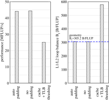
Figure 3: Performance of list-aa-pv-aos on one core of BDW-S system with and without padding as well as padding used to provoke cache and (L1) TLB thrashing. Benchmark geometry is channel containing $4\,802\,000$ fluid nodes.

Depending on the number of fluid nodes, SoA based kernels can suffer from cache and/or TLB thrashing which is described for full-array kernels e. g. in [29] and for list-based kernels in e. g. in [31]. For the SoA data layout relevant is the distance between two PDFs of the same node. In case of the list approach this is the number of fluid nodes. If this number maps the cache lines containing the relevant PDFs to only a subset of cache sets, which number of ways is not enough to hold them all, then thrashing occurs. During the process of a node update $19$ ($38$) cache lines for the AA pattern (OS-based kernels) must be held concurrently in cache. The BDW-S system’s L1 and L2 cache have only eight ways which already can be critical. TLB thrashing is based on the same effect only that the relevant unit is not cache lines, but pages. Depending on which page size is used, small $4$ KiB or huge $2$ MiB pages, different TLBs might exists. With padding, we ensure that cache lines are distributed over the sets by introducing additional nodes which are only used for spacing and are not updated.

Figure 3 shows the impact of cache and first level TLB thrashing on the BDW-S system. The channel geometry with $500\times 100\times 100$ nodes contains $4\,802\,000$ fluid nodes which spreads the cache lines and TLB entries over enough sets, hence no difference between with and without padding is observed. However, if we pad for cache and TLB thrashing, performance decreases nearly by $50$ % and the measured loop balance between L1 and L2 cache increases far above the theoretical $B_{l}=305.2$ B/FLUP for this geometry. Furthermore, first level TLB misses go from practically zero misses/FLUP to around $2.8$ misses/FLUP. The number of page-walks caused, i. e. the actual number of full page table lookups performed to translate the virtual to physical addresses, does not differ, as the second level TLB on this architecture is large enough. This was different for pre Haswell microarchitectures which only had a first level TLB for huge pages.

For all list-based kernels by default an automatic padding is activated, where we try to avoid cache/TLB thrashing. We assume a TLB cache for $2$ MiB pages with four sets and a cache with cache line size $=64$ B and $512$ sets. This resembles current Intels first level TLB and L2 cache configurations and might be counterproductive for other architectures, but can be adjusted by the user on the command line.

4.5 Heterogeneous Geometries

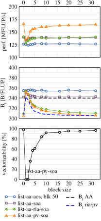
Figure 4: Performance of list-aa kernels with blocks geometry on ten cores of BDW-S system when the size of blocks is increased. Geometry dimensions are $500\times 100\times 100$ nodes.

Until now we only used the channel geometry , i. e. a homogeneous geometry, for benchmarking where nearly no boundary handling in form of bounce back was necessary as nearly the whole domain consists of fluid nodes. Furthermore, this homogeneity causes (i) a low loop balance for list-aa-ria-soa and list-aa-pv-soa and (ii) guarantees that most fluid nodes can be updated vectorized in case of list-aa-pv-soa’s odd time step.

Figure 4 shows the performance of the list AA kernels on one socket of the BDW-S system for the block geometry when the size of the blocks is increased. The simple list-aa-aos and list-aa-soa kernels show nearly the same performance independently of the geometries’ structures as their loop balance is constant. For small blocks all SoA kernels show a drop in performance for several reasons. The small blocks have an opposite effect on list-aa-ria-soa and list-aa-pv-soa, which use the run length coding RIA. Instead of having large number of consecutive fluid nodes in an empty channel, with small blocks the consecutive chunks become very short. This requires more storage for the run length coding and increases the loop balance. The theoretical values, shown as green dashed line in the middle panel of Fig. 4, is approximately reached by both implementations (green and orange lines). The performance drop is much more pronounced for list-aa-pv-soa. Nearly no fluid nodes can be updated vectorized during the odd time step with small blocks as shown in the lower panel of Fig. 4.

5 Socket Performance Results on Different Architectures

name		IVB	HSW-S	HSW-D	BDW-S	SKX	ZEN-S	ZEN-D
processor		Intel Xeon	Intel Xeon	Intel Xeon	Intel Xeon	Intel Xeon	AMD	AMD
name		E5-2660 v2	E5-2695 v3	E3-1240 v3	E5-2630 v4	Gold 6148	EPYC	Ryzen 7
							7451	1700X
micro.		Ivy Bridge	Haswell	Haswell	Broadwell	Skylake	Zen	Zen
freq	[GHz]	2.2	2.3	3.4	2.2	2.4	2.3	3.4
cores		10	2 $\times$ 7	4	10	20	24	8
ISA		AVX	AVX2	AVX2	AVX2	AVX-512	AVX2	AVX2
NUMA LDs		1	2	1	1	1	4	1
L1	[KiB]	32	32	32	32	32	32	32
L2	[KiB]	256	256	256	256	1024	512	512
L3	[MiB]	25	2 $\times$ 17.5	8	25	28	8 $\times$ 8	2 $\times$ 8
socket bandwidth
copy	[GB/s]	39.2	52.0	22.4	53.9	102.8	130.9	29.7
copy-19	[GB/s]	32.7	47.3	18.8	48.0	89.7	111.9	27.2
copy-19-nt-sl	[GB/s]	35.6	47.1	19.9	48.2	92.4	111.7	27.1
update-19	[GB/s]	37.4	44.0	19.2	51.1	93.6	109.2	26.1
sockets		2	2	1	2	2	2	1

Table 3: Specification of systems used for full socket measurements. Number of cores specifies the physical cores and the number of NUMA locality domains (LD) are given per socket. The copy and copy-19 bandwidths already accounts for the write allocate. copy-19-nt-sl uses non-temporal stores. On HSW-S cluster-on-die mode is enabled.

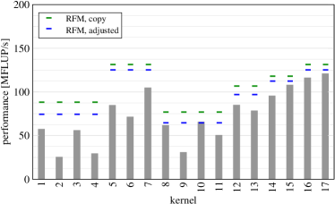
(a) IVB, 10 cores, AVX

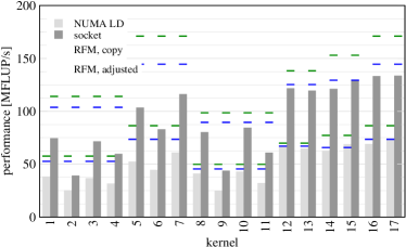
(b) HSW-S, 14 cores, AVX2

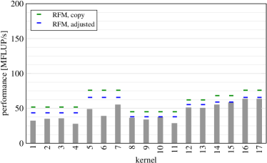
(c) HSW-D, 4 cores, AVX2

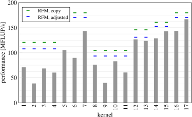
(d) BDW-S, 10 cores, AVX2

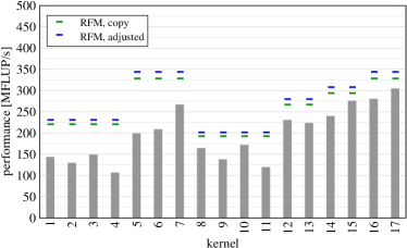
(e) SKX, 20 cores, AVX2

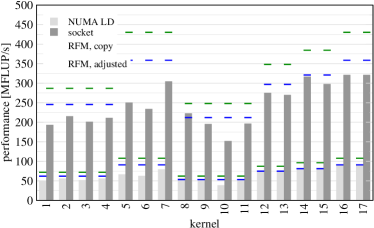
(f) ZEN-S, 24 cores, AVX

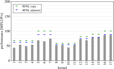
(g) ZEN-D, 8 cores, AVX

1	blk-push-aos		10	list-pull-aos
2	blk-push-soa		11	list-pull-soa
3	blk-pull-aos		12	list-pull-split-nt-s1
4	blk-pull-soa		13	list-pull-split-nt-s2
5	aa-aos		14	list-aa-aos
6	aa-soa		15	list-aa-soa
7	aa-vec-soa		16	list-aa-ria-soa
8	list-push-aos		17	list-aa-pv-soa
9	list-push-soa

(h) legend

Figure 5: Full socket measurements of implemented kernels with channel geometry of dimensions $500\times 100\times 100$ nodes on different hardware architectures. Kernels supporting blocking several blocking factors are measured, but only the measurement of the one which resulted in the best performance is reported. Table LABEL:sub@fig:p:fm:legend shows the kernels for the corresponding indices of the plots. Please note the different scaling on the y axis.

In this section we evaluate the kernels’ performance on full sockets of several hardware architectures specified in Table 3. Although most systems comprising two sockets, we limit the study to only one. Despite trying to respect the first-touch policy and thereby being NUMA-aware, this only works to a certain degree as we will see later on. Hence, a typical setup for these machines would be using an hybrid OpenMP/MPI parallel code, where per socket one MPI process is run. The OpenMP parallel part for such a code, could stem for example from this suite.

As noted in the previous Sect., we fix the cores’ frequency to the nominal frequency, pin each thread, use Intel C Compiler 17.0.1, and set the target architecture to compile for to AVX or AVX2, where supported.

In the following we highlight relevant details of the used machines. BDW-D and ZEN-D resemble “desktop” like versions of the processors, which can nearly saturate the memory bandwidth with one core, but do not show a difference with utilizing all cores. For the other machines multiple cores are required to staturate the memory bandwidth. All machines except BDW-S and HSW-D have SMT enabled, but we always use the physical cores only. Furthermore, HSW-S and ZEN-S exhibit several NUMA locality domains per socket. For these architectures we report also the performance of such a single domain. HSW-S is operated in cluster-on-die (CoD) mode, where the processor is logically divided into two halfs and each half has its own share of the L3 cache and its own NUMA doamin. Three cores of ZEN-S share a separate part of the L3 cache. Two such complexes, i. e. six cores build one NUMA domain. The Skylake SKX system supports AVX-512. However, currently the kernels only support AVX2, why all reported numbers for this system are measured with AVX2. We also do not expect any benefit from AVX-512 on this machine as these instructions are executed with a lower clock frequency and the highly optimized kernels nearly meet the performance pedictions, i. e. saturate the memory bandwidth. On Knights Landing based system, the High Bandwidth Memory (HBM) exhibits a significantly higher bandwidth than the one achievable from DRAM. Here the situation might be different. It is also the only system where multi-stream memory benchmarks copy-19, copy-19-nt-sl, and update-19 are faster than the single stream benchmark copy. The AMD Zen based systems ZEN-S and ZEN-D support AVX2. However, measurements on ZEN-S show a slight performance advantage of the kernels when AVX-only code (without FMA) is used. For ZEN-D no difference is measurable.

The kernels’ performance on the different machines is found in Fig. 5. The graphs show in green and blue lines the performance limit according to the Roofline model from Sec. 4.1. Hereby for the green lines the copy bandwidth is used, whereas for the blue lines a micro-benchmark is used which more resembles the kernels access pattern like copy-19, copy-19-nt-sl, or update-19. Which bandwidth is used for which kernel is found in Table 1.

As geometry channel with $500\times 100\times 100$ nodes is used. For kernels supporting blocking several blocking factors are used, but only the one which results in the best performance is reported.

In general list-aa-pv-soa exhibits the best performance on all evaluated machines. Whether the non-vectorized version list-aa-ria-soa with an equal loop balance reaches the same performance depends on the architectures. The reason for this is unclear and needs further investigation. The vectorization in list-aa-pv-soa has actually the effect of saturating the performance with less cores. With all cores no difference should be visible as e. g. HSW-S in Fig. 5b exhibits. There is not pattern for the performance behavior of list-aa-aos/-soa. On HSW-S/-D (Fig. 5b and 5c) and ZEN-S/-D (Fig. 5f and 5g) they nearly match the performance of their optimized siblings, whereas on the other machines a larger gap is visible. The vectorized full array kernel of AA aa-vec-soa reaches despite the slightly lower loop balance not the performance of list-aa-pv-soa. Altering the geometry dimensions (not shown), especially increasing the inner dimension, reveals a significantly higher performance. As measurements of L2 traffic, branch misspredictions, TLB misses, and performed page walks for different dimensions show no abnormalities, we speculate that the relatively short inner dimension of $100$ might be the cause. The optimization for vector machines as proposed in [29], where the loop nest iterating over the three spatial dimensions is fused into one, could here be beneficial. The one step kernels with non-temporal stores list-pull-split-nt-(s1/s2)-soa can be ranked after the optimized AA pattern kernels. The measurements show that there is practically no difference between using one or two non-temporal store streams. The slowest kernels, as expected by the highest loop balance, are the unoptimized versions of the one step propagation step. They show the tendency that the list implementations have a slight advantage. The measurements however, do not allow for a decision whether SoA or AoS (with blocking) data layout reaches in general a higher performance.

Typically the bandwidth scales linearly over NUMA locality domains if first-touch policy is respected. However, one effect that causes non-perfect scaling for the kernels are pages which are part of two subdomains that are placed in separate NUMA LDs. This is the case when a memory page boundary is not aligned to its subdomain boundary. Each core updates a separate subdomain. The core which first touches this page places it into its NUMA LD. On HSW-S with CoD mode enabled two NUMA LDs exists. All except for one kernel reach between $90$ and $99$ % of the performance when we assume the performance of one NUMA LD scales perfectly. Only blk-push-soa reaches only $78$ %. The reason for this is unclear and needs further investigation. On the ZEN-S system with four NUMA domains all kernels reach $90$–$99$ % of the projected performance from one NUMA domain.

6 Conclusion

We introduced the lattice Boltzmann benchmark kernels, a suite for benchmarking simple LBM kernels, which may be used for performance experiments or can act as a blue print for an implementation. An initial set of kernels is already implemented, which range from simple to highly optimized ones. Thereby widely used data layouts and lattice representations are covered. The kernels’ performance behavior was evaluated by strong scaling on one socket of a Broadwell based architecture and effects like loop blocking, array padding, and impact of heterogeneous domains were discussed. By the usage of the Roofline performance model we were able to determine a performance limit for each kernel. Finally, the kernels were compared on different current hardware architectures.

We plan to add more optimized kernels, especially with full array as lattice representation. These also offer simple ways regarding temporal blocking. The full array kernels are currently missing a padding mechanism, which will be implemented, as it is crucial for avoiding cache/TLB thrashing. Currently the porting of the list-aa-pv-soa kernel to Intel’s Knights Landing architecture is ongoing and will make use of AVX-512 instruction including gather and scatter operations.

References

- [1] P. Bailey, J. Myre, S. Walsh, D. Lilja, and M. Saar. Accelerating lattice Boltzmann fluid flow simulations using graphics processors. In International Conference on Parallel Processing 2009 (ICPP’09), pages 550–557, Sept 2009. doi:10.1109/ICPP.2009.38.
- [2] M. Bernaschi, S. Succi, M. Fyta, E. Kaxiras, S. Melchionna, and J. Sircar. MUPHY: A parallel high performance MUlti PHYsics/Scale code. In IEEE International Symposium on Parallel and Distributed Processing, 2008. IPDPS 2008., April 2008. doi:10.1109/IPDPS.2008.4536464.
- [3] H. Chen, S. Chen, and W. H. Matthaeus. Recovery of the Navier-Stokes equations using a lattice-gas Boltzmann method. Phys. Rev. A, 45:5339–5342, Apr 1992. doi:10.1103/PhysRevA.45.R5339.
- [4] D. d’Humières, I. Ginzburg, M. Krafczyk, P. Lallemand, and L. Luo. Multiple-relaxation-time lattice Boltzmann models in three dimensions. Phil. Trans. R. Soc. Lond. A, 360(1792):437–451, mar 2002. doi:10.1098/rsta.2001.0955.
- [5] S. Donath, T. Zeiser, G. Hager, J. Habich, and G. Wellein. Optimizing performance of the lattice boltzmann method for complex structures on cache-based architectures. In Frontiers in Simulation: Simulation Techniques - 18th Symposium in Erlangen, September 2005 (ASIM), pages 728–735. SCS Publishing House, 2005.
- [6] C. Feichtinger, S. Donath, H. Köstler, J. Götz, and U. Rüde. WaLBerla: HPC software design for computational engineering simulations. Journal of Computational Science, 2(2):105–112, 2011. doi:10.1016/j.jocs.2011.01.004.
- [7] S. Freudiger, J. Hegewald, and M. Krafczyk. A parallelisation concept for a multi-physics lattice Boltzmann prototype based on hierarchical grids. Computational Fluid Dynamics, 8(1–4):168–178, 2008. doi:10.1504/PCFD.2008.018087.
- [8] I. Ginzburg, F. Verhaeghe, and D. d’Humières. Two-relaxation-time lattice Boltzmann scheme: About parametrization, velocity, pressure and mixed boundary conditions. Commun. Comput. Phys., 3(2):427–428, 2008.
- [9] J. Habich. A Performance Engineering Process for Developing High Performance Lattice Boltzmann Implementations. PhD thesis, Friedrich-Alexander-Universität Erlangen-Nürnberg, 2015.
- [10] J. Habich, T. Zeiser, G. Hager, and G. Wellein. Enabling temporal blocking for a lattice Boltzmann flow solver through multicore aware wavefront parallelization. In International Conference on Parallel Computational Fluid Dynamics 2009 (Parallel CFD 2009), pages 178–182, May 2009.
- [11] D. Hänel. Molekulare Gasdynamik. Springer, 2004.
- [12] F. H. Harlow and J. E. Welch. Numerical calculation of time-dependent viscous incompressible flow of fluid with free surface. Phys. Fluids, 8(2182), 1965. doi:10.1063/1.1761178.
- [13] M. Hasert, K. Masilamani, S. Zimny, H. Klimach, J. Qi, J. Bernsdorf, and S. Roller. Complex fluid simulations with the parallel tree-based lattice Boltzmann solver Musubi. J. Comp. Sci., 2013. doi:10.1016/j.jocs.2013.11.001.
- [14] J. Linxweiler. Ein integrierter Softwareansatz zur interaktiven Exploration und Steuerung von Strömungssimulationen auf Many-Core-Architekturen. PhD thesis, Fakultät Architektur, Bauingenieurwesen und Umweltwissenschaften, TU-Braunschweig, 2011.
- [15] N. S. Martys and J. G. Hagedorn. Multiscale modeling of fluid transport in heterogeneous materials using discrete Boltzmann methods. Mater. Struct, 35:650–659, 2002.
- [16] J. D. McCalpin. Memory bandwidth and machine balance in current high performance computers. IEEE Computer Society Technical Committee on Computer Architecture (TCCA) Newsletter, pages 19–25, Dec. 1995.
- [17] A. Nguyen, N. Satish, J. Chhugani, C. Kim, and P. Dubey. 3.5-D blocking optimization for stencil computations on modern cpus and gpus. In Proceedings of the 2010 ACM/IEEE International Conference for High Performance Computing, Networking, Storage and Analysis, SC ’10, Washington, DC, USA, 2010. IEEE Computer Society. doi:10.1109/SC.2010.2.
- [18] C. Pan, J. F. Prins, and C. T. Miller. A high-performance lattice Boltzmann implementation to model flow in porous media. Computer Physics Communications, 158(2):89–105, 2004. doi:10.1016/j.cpc.2003.12.003.
- [19] A. Pasquali, M. Schönherr, M. Geier, and M. Krafczyk. Simulation of external aerodynamics of the DrivAer model with the LBM on GPGPUs. In G. R. Joubert, H. Leather, M. Parsons, F. Peters, and M. Sawyer, editors, Parallel Computing: On the Road to Exascale, volume 27 of Advances in Parallel Computing, pages 391–400. IOS Press, 2016. doi:10.3233/978-1-61499-621-7-391.
- [20] T. Pohl, M. Kowarschik, J. Wilke, K. Iglberger, and U. Rüde. Optimization and profiling of the cache performance of parallel lattice Boltzmann codes. Parallel Processing Letters, 13(4):549–560, 2003. doi:10.1142/S0129626403001501.
- [21] Y. H. Qian, D. d’Humières, and P. Lallemand. Lattice BGK models for Navier-Stokes equation. EPL (Europhysics Letters), 17(6):479, 1992. doi:10.1209/0295-5075/17/6/001.
- [22] M. Schönherr. Towards reliable LES-CFD computations based on advanced LBM models utilizing (Multi-) GPGPU hardware. PhD thesis, Fakultät Architektur, Bauingenieurwesen und Umweltwissenschaften, TU-Braunschweig, 2015.
- [23] M. Schönherr, M. Geier, and M. Krafczyk. 3D GPGPU LBM implementation on non-uniform grids. In International Conference on Parallel Computational Fluid Dynamics 2011 (Parallel CFD 2011), May 2011.
- [24] M. Schulz, M. Krafczyk, J. Tölke, and E. Rank. Parallelization strategies and efficiency of CFD computations in complex geometries using lattice Boltzmann methods on high performance computers. In M. Breuer, F. Durst, and C. Zenger, editors, High Performance Scientific and Engineering Computing Proceedings of the 3rd International FORTWIHR Conference on HPSEC, Erlangen, March 12-14, 2001, volume 21 of Lecture Notes in Computational Science and Engineering, pages 115–122, Berlin, Heidelberg, 2002. Springer-Verlag. doi:10.1007/978-3-642-55919-8_13.
- [25] J. Treibig, G. Hager, and G. Wellein. LIKWID: A lightweight performance-oriented tool suite for x86 multicore environments. In Proceedings of the 2010 39th International Conference on Parallel Processing Workshops, ICPPW ’10, pages 207–216, Washington, DC, USA, 2010. IEEE Computer Society. doi:10.1109/ICPPW.2010.38.
- [26] D. Vidal, R. Roy, and F. Bertrand. On improving the performance of large parallel lattice Boltzmann flow simulations in heterogeneous porous media. Computers & Fluids, 39(2):324–337, 2010. doi:10.1016/j.compfluid.2009.09.011.
- [27] J. Wang, X. Zhang, A. G. Bengough, and J. W. Crawford. Domain-decomposition method for parallel lattice Boltzmann simulation of incompressible flow in porous media. Phys. Rev. E, 72(1), 2005. doi:10.1103/PhysRevE.72.016706.
- [28] G. Wellein, G. Hager, T. Zeiser, M. Wittmann, and H. Fehske. Efficient temporal blocking for stencil computations by multicore-aware wavefront parallelization. In Proceedings of the 33rd IEEE International Computer Software and Applications Conference (COMPSAC 2009), pages 579–586, 2009. doi:10.1109/COMPSAC.2009.82.
- [29] G. Wellein, T. Zeiser, S. Donath, and G. Hager. On the single processor performance of simple lattice Boltzmann kernels. Computers & Fluids, 35:910–919, 2006. doi:10.1016/j.compfluid.2005.02.008.
- [30] S. Williams, A. Waterman, and D. Patterson. Roofline: an insightful visual performance model for multicore architectures. Commun. ACM, 52(4):65–76, Apr 2009. doi:10.1145/1498765.1498785.
- [31] M. Wittmann. Hardware-effiziente, hochparallele Implementierungen von Lattice-Boltzmann-Verfahren für komplexe Geometrien. Dissertation, Friedrich-Alexander-Universität Erlangen-Nürnberg, 2016.
- [32] M. Wittmann, G. Hager, T. Zeiser, J. Treibig, and G. Wellein. Chip-level and multi-node analysis of energy-optimized lattice Boltzmann CFD simulations. Concurrency and Computation: Practice and Experience, 2015. doi:10.1002/cpe.3489.
- [33] M. Wittmann, T. Zeiser, G. Hager, and G. Wellein. Comparison of different propagation steps for lattice Boltzmann methods. Computers & Mathematics with Applications, 65(6):924–935, 2013. doi:10.1016/j.camwa.2012.05.002.
- [34] M. Wittmann, T. Zeiser, G. Hager, and G. Wellein. Modeling and analyzing performance for highly optimized propagation steps of the lattice Boltzmann method on sparse lattices. CoRR, abs/1410.0412v2, 2015. Version 2: arXiv:1410.0412v2.
- [35] T. Zeiser, G. Hager, and G. Wellein. Benchmark analysis and application results for lattice Boltzmann simulations on NEC SX vector and Intel Nehalem systems. Parallel Processing Letters, 19(4):491–511, 2009. doi:10.1142/S0129626409000389.