Interesting examples of violation of the classical equivalence principle but not of the weak one

Abstract

The equivalence principle (EP), as well as Schiff’s conjecture, are discussed en passant, and the connection between the EP and quantum mechanics is then briefly analyzed. Two semiclassical violations of the classical equivalence principle (CEP) but not of the weak one (WEP), i.e. Greenberger gravitational Bohr atom and the tree-level scattering of different quantum particles by an external weak higher-order gravitational field, are thoroughly investigated afterwards. Next, two quantum examples of systems that agree with the WEP but not with the CEP, namely COW experiment and free fall in a constant gravitational field of a massive object described by its wave-function $\Psi$, are discussed in detail. Keeping in mind that among the four examples focused on this work only COW experiment is based on an experimental test, some important details related to it, are presented as well.

I Introduction

The equivalence principle (EP) is intrinsically connected to the history of gravitation theory and has played an important role in its development. Newton regarded this principle as such a cornerstone of mechanics that he devoted the opening paragraph of the Principia to it.

Let us then discus, in passing, some important aspects related to the EP in the framework of both Newton and Einstein gravity.

The classical equivalence principle (CEP) of Newtonian theory (universality of free fall, or equality of inertial and gravitational masses) has a nonlocal character. As far as Einstein gravity is concerned two EP are generally contemplated: the weak equivalence principle (WEP) and the Einstein one (EEP). The WEP asserts that locally we cannot distinguish between inertial and gravitational fields through ‘falling body experiments’. Since the WEP, as well as the CEP, are locally identical, the difficult, at the first sight, of differentiating them in an easy way increases. Consequently, some researchers are led to the common misconception that they coincide even nonlocally (see for instance 1 ; 2 ; 3 ; 4 ; 5 ). EEP, on the other hand, embodies WEP, local Lorentz invariance — the outcome of any local non-gravitational experiment is independent of the velocity of the freely-falling reference frame in which it is performed — and local position invariance — the outcome of any local non-gravitational experiment is independent of where and when it is performed 6 . EEP may be considered in the broadest sense of the term as the heart and soul of gravity theory. It would not be an exaggeration to say that if the EEP holds, then gravitation must necessarily be a ‘curved spacetime’ phenomenon; in other words, the effects of gravity must be equivalent to the effects of living in a curved spacetime 6 . Around 1960, Schiff conjectured that any complete and self consistent theory of gravity that obeys the WEP must also, unavoidable, obey the EEP 7 . This surmise is known as Schiff’s conjecture. According to it the validity of the WEP alone should guarantee the validity of the local Lorentz and position invariance, and thus of the EEP. However, a rigorous proof of Schiff’s conjecture is improbable. In fact, some special counterexamples are available in the literature 8 ; 9 ; 10 ; 11 . Nevertheless, there are some powerful arguments of ‘plausibility’, such as the assumption of energy conservation 12 and the $TH\epsilon\mu$ formalism 13 , among others, that can be formulated.

A natural question must now be posed: what is the connection between the EP and quantum mechanics? As is well known, quantum tests of the EP are radically different from the classical ones because classical and quantum descriptions of motion are fundamentally unlike. In particular, the universality of free fall (UFF) possesses a clear significance in the classical context. Now, how both UFF and WEP are to be understood in quantum mechanics is a much more subtle point. It is generally implicitly assumed that quantum mechanics is valid in the freely falling frame associated with classical test bodies. Nonetheless, an unavoidable problem regarding quantum objects is the existence of half integer spins, which have no classical counterpart. For integer spin particles, the EP can be accounted for by a minimal coupling principle (see subsections A.1 and A.3 of Appendix A); while the procedure to couple a spin $1/2$ field to gravity is much more complex and requires the use of a spinorial representation of the Lorentz group (see subsection A.2 of Appendix A).

On the other hand, the most cited scientific experiment claimed to support the idea that, at least in some cases, quantum mechanics and the WEP can be reconciled, is COW experiment 2 . Although this test, as we shall prove, is in accord with the WEP, it is in disagreement with the CEP. Another example of a possible quantum mechanical violation of the CEP but not of the WEP is provided by analyzing free fall in a constant gravitational field of a massive object described by its wave-function $\Psi$.

At the semiclassical level an interesting event in which the CEP is also supposed to be violated but not the WEP is the tree level deflection of different quantum particles by an external weak higher-order gravitational field. We recall beforehand that in Einstein theory the scattering of any particle by an external weak gravitational field is nondispersive which, of course, is in agreement with the WEP. In other words, the deflection angle of all massive particles will be exactly equal. The same is valid for the massless particles. Obviously, the deflection angle will be different whether the particle is massive or massless. A crucial question must then be posed: why to study at the tree level the bending of quantum particles in the framework of higher-derivative gravity? It is not difficult to answer this question. Higher-derivative gravity is the only model that is known to be renormalizable along its matter couplings up to now 14 . Nonetheless, since this system is renormalizable, it is compulsorily nonunitary 15 ; 16 . We call attention to the fact that the breaking down of unitarity is indeed a serious problem. Fortunately, we shall only deal with the linearized version of higher-derivative gravity, which is stable 17 . The reason why it does not explode is because the ghost cannot accelerate owing to energy conservation. Another way of seeing this is by analyzing the free-wave solutions. We remark that this model is not in disagreement with the result found by Sotiriou and Faraoni 18 . In fact, despite containing a massive spin-2 ghost, as asserted by these authors, the alluded ghost cannot cause trouble 19 . Another probable example at the tree level of violation of the CEP but not of the WEP is provided by Greenberger gravitational Bohr atom 1 .

Our main goal here is to explicitly show that in all situations described above, the WEP is not violated but the CEP is.

The article is organized as follows.

In Section 2 we study the following semiclassical examples:

• Greenberger gravitational Bohr atom.

• Tree-level scattering of different quantum particles by an external weak higher-order gravitational field.

After a careful investigation of both models, we came to the conclusion that they do not violate at all the WEP but are not in accord with the CEP. As far as the second example is concerned, it is worthy of note that the resulting deflection angles are dependent on both spin and energy. In addition the well known deflection angles (related to both massive and massless particles) predicted by general relativity are recovered through a suitable limit process.

In Section 3 we analyze two quantum examples: COW experiment and free fall in a constant gravitational field of a massive object described in quantum mechanics by the wave-function $\Psi$. Again, these systems are in accord with the WEP but not with the CEP.

Our comments are presented in Section 4.

The lengthy calculations concerning the computation of unpolarized cross sections for the scattering of different quantum particles by an external weak higher-order gravitational field are put in Appendix A.

We use natural units throughout and our Minkowski metric is diag(1, -1, -1 ,-1).

II Two examples of semiclassical violation of the CEP but not of the WEP

We analyze in the following two examples of semiclassical violation of the CEP but not of the WEP in a gravitational field.

II.1 Greenberger gravitational Bohr atom

As far as we know, Greenberger 1 was the first to foresee the existence of mass-dependent interference effects related to a particle bound in an external gravitational field.

Here we are particularly interested in analyzing Greenberger gravitational Bohr atom, which from the classical point of view consists of a small mass $m$ bound to a very much larger mass $M$ by the potential $V(r)=-\frac{GMm}{r}$, in the limit where all recoil effects may be neglected. If we restrict ourselves to circular orbits, we arrive at the conclusion that classically $\omega^{2}r^{3}=GM$ (see figure 1).

From this point on Greenberger applied the same postulate proposed by Bohr:

‘The particles move in orbits restricted by the requirement that the angular momentum be an integer multiple of $\hbar$’. Therefore, according to this postulate for circular orbits of radius $r$ the possible values of $r$ are restricted by $L=mr^{2}\omega=n$ , so that

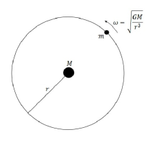
Figure 1: Greenberger classical gravitational Bohr atom with circular orbit.

$$\omega_{n}=\frac{(GM)^{2}m^{3}}{n^{2}},\;\;r_{n}=\frac{n^{2}}{GMm^{2}},\;\;E_{n}=\frac{(GM)^{2}m^{3}}{2n^{2}}.$$ (1)

From the equations above, we see that lowest Bohr radius varies as $\frac{1}{m^{2}}$, and the orbital frequency as $m^{3}$. As a consequence, it would be trivial to tell the mass of the orbiting particle merely by observing its radius. This result, of course, is in contradiction with what is expected from Newtonian gravity and the CEP. Nonetheless, there is no conflict between this result and the WEP. In fact, the WEP, as we have already mentioned, is a pure local statement, while Greenberger gravitational Bohr atom is an object extended in space. Note however that the gravitational Bohr atom is not a fully quantum system but only a semiquantum or semiclassical one, exactly as it happens with the original Bohr’s atom model, where according to the aforementioned postulate the orbiting object has a well definite trajectory and in addition there is the extra ad hoc assumption of quantization of the angular momentum. In a fully quantum mechanical treatment, a probability of presence is obtained via the wave-function, the ‘uncertainty principle’ expressing the link between the width of the mentioned wave-function in both the direct and reciprocal spaces.

II.2 Tree-level deflection of different quantum particles by an external weak higher-order gravitational field

The action for higher-order gravity can be written as

$$I=\int\sqrt{-g}\Big{[}\frac{2}{\kappa^{2}}R+\frac{\alpha}{2}R^{2}+\frac{\beta}{2}R^{2}_{\mu\nu}\Big{]}-I_{\mathrm{M}},$$ (2)

where $\kappa^{2}=32\pi G$, with $G$ being Newton’s constant, $\alpha$ and $\beta$ are free dimensionless coefficients, and $I_{\mathrm{M}}$ is the action for matter.

The field equations concerning the action above are

$$\frac{2}{\kappa^{2}}G_{\mu\nu}+\frac{\beta}{2}\Big{[}-\frac{1}{2}g_{\mu\nu}R^{2}_{\rho\lambda}+\nabla_{\mu}\nabla_{\nu}R+2R_{\mu\rho\lambda\nu}R^{\rho\lambda}$$

$$-\frac{1}{2}g_{\mu\nu}\Box R-\Box R_{\mu\nu}\Big{]}+\frac{\alpha}{2}\Big{[}-\frac{1}{2}g_{\mu\nu}R^{2}+2RR_{\mu\nu}$$

$$+2\nabla_{\mu}\nabla_{\nu}R-2g_{\mu\nu}\Box R\Big{]}+\frac{1}{2}\Theta_{\mu\nu}=0,$$

where $\Theta_{\mu\nu}$ is the energy-momentum tensor.

From the above equation we promptly obtain its linear approximation doing exactly as in Einstein’s theory, i.e. we write

$$g_{\mu\nu}=\eta_{\mu\nu}+\kappa h_{\mu\nu},$$ (3)

and then linearize the equation at hand via (3), which results in the following

$$\Big{(}1-\frac{\beta\kappa^{2}}{4}\Box\Big{)}\Big{[}-\frac{1}{2}\Box h_{\mu\nu}+\frac{1}{6\kappa}R^{(\mathrm{lin})}\eta_{\mu\nu}\Big{]}+\frac{1}{2}(\Gamma_{\mu,\nu}$$

$$+\Gamma_{\nu,\mu})=\frac{\kappa}{4}\Big{(}T_{\mu\nu}-\frac{1}{3}T\eta_{\mu\nu}\Big{)},$$

where

$$R^{(\mathrm{lin})}=\frac{\kappa}{2}\Box h-\kappa{\gamma^{\mu\nu}}_{,\mu\nu},$$

$$\gamma_{\mu\nu}\equiv h_{\mu\nu}-\frac{1}{2}\eta_{\mu\nu}h,$$

$$\Gamma_{\mu}\equiv\Big{(}1-\frac{\beta\kappa^{2}}{4}\Box\Big{)}{\gamma_{\mu\nu}}^{,\nu}-\Big{(}\alpha+\frac{\beta}{2}\Big{)}\frac{\kappa}{2}{R^{(\mathrm{lin})}}_{,\mu}.$$

Note that indices are raised (lowered) using $\eta^{\mu\nu}$ ($\eta_{\mu\nu}$). Here $T_{\mu\nu}$ is the energy-momentum tensor of special relativity.

It can be shown that it is always possible to choose a coordinate system such that the gauge conditions, $\Gamma_{\mu}=0$, on the linearized metric hold. Assuming that these conditions are satisfied, it is straightforward to show that the general solution of the linearized field equations is given by 20 ; 21

$$h_{\mu\nu}=h^{({\mathrm{E}})}_{\mu\nu}-\phi\eta_{\mu\nu}+\psi_{\mu\nu},$$ (4)

where $h^{({\mathrm{E}})}_{\mu\nu}$ is the solution of linearized Einstein’s equations in the de Donder gauge, i.e.,

$$\Box h^{({\mathrm{E}})}_{\mu\nu}=\frac{\kappa}{2}\Big{[}\frac{T\eta_{\mu\nu}}{2}-T_{\mu\nu}\Big{]},\;\;\;\gamma^{{({\mathrm{E}})\;,\nu}}_{\mu\nu}=0,$$

$$\gamma^{{({\mathrm{E}})}}_{\mu\nu}\equiv h^{({\mathrm{E}})}_{\mu\nu}-\frac{1}{2}\eta_{\mu\nu}h^{({\mathrm{E}})},$$

while $\phi$ and $\psi_{\mu\nu}$ satisfy, respectively, the equations

$$\Big{(}\Box+m^{2}_{0}\Big{)}\phi=\frac{\kappa T}{12},$$

$$\Big{(}\Box+m^{2}_{2}\Big{)}\psi_{\mu\nu}=\frac{\kappa}{2}\Big{[}T_{\mu\nu}-\frac{1}{3}T\eta_{\mu\nu}\Big{]},\;\Box\psi={\psi_{\mu\nu}}^{,\mu\nu}.$$

It is worthy of note that in this very special gauge the equations for $\psi_{\mu\nu},\;\phi,\;$ and $h^{({\mathrm{E}})}_{\mu\nu}$ are totally decoupled. As a result, the general solution to the linearized field equations reduces to an algebraic sum of the solutions of the equations concerning the three mentioned fields.

Solving the preceding equations for a pointlike particle of mass $M$ located at ${\bf r=0}$ and having, as a consequence, an energy momentum tensor $T_{\mu\nu}=M\eta_{\mu 0}\eta_{\nu 0}\delta^{3}({\bf r})$, we find

$$h_{\mu\nu}(r)=h^{(\mathrm{E})}_{\mu\nu}(r)+h^{(\mathrm{R^{2}})}_{\mu\nu}(r)+h^{\mathrm{(R_{\mu\nu}^{2})}}_{\mu\nu}(r),$$ (5)

with

$$h^{(\mathrm{E})}_{\mu\nu}(r)=\frac{M\kappa}{16\pi}\Big{[}\frac{\eta_{\mu\nu}}{r}-\frac{2\eta_{\mu 0}\eta_{\nu 0}}{r}\Big{]},$$

$$h^{(\mathrm{R^{2}})}_{\mu\nu}(r)=\frac{M\kappa}{16\pi}\Big{[}-\frac{1}{3}\frac{e^{-m_{0}r}}{r}\eta_{\mu\nu}\Big{]},$$

$$h^{\mathrm{(R_{\mu\nu}^{2})}}_{\mu\nu}(r)=\frac{M\kappa}{16\pi}\Big{[}-\frac{2}{3}\frac{e^{-m_{2}r}}{r}\eta_{\mu\nu}+2\frac{e^{-m_{2}r}}{r}\eta_{\mu 0}\eta_{\nu 0}\Big{]}.$$

Note that for $m_{0},\;m_{2}\rightarrow\infty$, the above solution reproduces the solution of linearized Einstein field equations in the de Donder gauge, as it should.

On the other hand, the momentum space gravitational field, namely $h^{\lambda\rho}_{\mathrm{ext}}({\bf{k}})$, is defined by

$$h^{\lambda\rho}_{\mathrm{ext}}({\bf{k}})=\int{d^{3}{\bf{r}}e^{-i{\bf{k}}\cdot{\bf{r}}}h^{\lambda\rho}_{\mathrm{ext}}({\bf{r}})}.$$ (6)

Thence,

$$h^{\lambda\rho}_{\mathrm{ext}}({\bf{k}})=h^{{\mathrm{(E)}}\lambda\rho}_{\mathrm{ext}}({\bf{k}})+h^{{\mathrm{(R^{2}_{\mu\nu})}}\lambda\rho}_{\mathrm{ext}}({\bf{k}})+h^{{\mathrm{(R^{2})}}\lambda\rho}_{\mathrm{ext}}({\bf{k}}),$$ (7)

with

$$h^{{\mathrm{(E)}}\mu\nu}_{\mathrm{ext}}({\bf{k}})=\frac{\kappa M}{4{\bf{k}}^{2}}\eta^{\mu\nu}-\frac{\kappa M}{2}\frac{\eta^{\mu 0}\eta^{\nu 0}}{\bf{\bf{k}}^{2}},$$

$$h^{{\mathrm{(R^{2}_{\alpha\beta})}}\mu\nu}_{\mathrm{ext}}({\bf{k}})=-\frac{\kappa M}{6}\frac{\eta^{\mu\nu}}{{\bf{k}}^{2}+m^{2}_{2}}+\frac{\kappa M}{2}\frac{\eta^{\mu 0}\eta^{\nu 0}}{{\bf{k}}^{2}+m^{2}_{2}},$$

$$h^{{\mathrm{(R^{2})}}\mu\nu}_{\mathrm{ext}}({\bf{k}})=-\frac{\kappa M}{12}\frac{\eta^{\mu\nu}}{{\bf{k}}^{2}+m^{2}_{0}}.$$

We are now ready to compute the tree-level scattering of different quantum particles by an external weak higher-order gravitational field. Nevertheless, since these calculations are very extensive, they were put in Appendix A.

The outcome of the experiments analyzed in Appendix A are summarized in Table 1 . A cursory glance at this table is enough to convince us that the unpolarized differential cross sections and, of course, the deflection angles, depend on the spin and energy of the scattered particle.

Table 1: Unpolarized differential cross sections for the tree-level scattering of different quantum particles by an external weak higher-order gravitational field, where $\theta$ is the scattering angle.

$m$	$s$	$\frac{d\sigma}{d\Omega}$
$0$	$0$	$\left(\frac{GM}{\sin^{2}\frac{\theta}{2}}\right)^{2}\Big{(}1+\frac{\sin^{2}\frac{\theta}{2}-3}{3(1+\frac{\lambda_{2}}{4}\csc^{2}\frac{\theta}{2})}-\frac{\sin^{2}\frac{\theta}{2}}{3(1+\frac{\lambda_{0}}{4}\csc^{2}\frac{\theta}{2})}\Big{)}^{2}$
$\neq 0$	$0$	$\left(\frac{GM}{\sin^{2}\frac{\theta}{2}}\right)^{2}\Big{(}1+\frac{\lambda}{2}+\frac{\sin^{2}\frac{\theta}{2}-(3+2\lambda)}{3(1+\frac{\lambda_{2}}{4}\csc^{2}\frac{\theta}{2})}-\frac{\sin^{2}\frac{\theta}{2}-\frac{\lambda}{2}}{3(1+\frac{\lambda_{0}}{4}\csc^{2}\frac{\theta}{2})}\Big{)}^{2}$
$0$	$\frac{1}{2}$	$\left(\frac{GM}{\sin^{2}\frac{\theta}{2}}\right)^{2}\cos^{2}\frac{\theta}{2}\Big{(}1-\frac{1}{1+\frac{\lambda_{2}}{4}\csc^{2}\frac{\theta}{2}}\Big{)}^{2}$
$\neq 0$	$\frac{1}{2}$	$\left(\frac{GM}{\sin^{2}\frac{\theta}{2}}\right)^{2}\sum_{n=0}^{2}\Big{[}\frac{E_{n}\lambda^{n}}{4}+\frac{A_{n}\lambda^{n}}{9(4+\lambda_{2}\csc^{2}\frac{\theta}{2})^{2}}+\frac{B_{n}\lambda^{n}}{9(4+\lambda_{0}\csc^{2}\frac{\theta}{2})^{2}}+\frac{C_{n}\lambda^{n}}{9(4+\lambda_{2}\csc^{2}\frac{\theta}{2})(4+\lambda_{0}\csc^{2}\frac{\theta}{2})}\Big{]}$
$0$	$1$	$\left(\frac{GM}{\sin^{2}\frac{\theta}{2}}\right)^{2}\cos^{4}\frac{\theta}{2}\Big{(}1-\frac{1}{1+\frac{\lambda_{2}}{4}\csc^{2}\frac{\theta}{2}}\Big{)}^{2}$
$\neq 0$	$1$	$\left(\frac{GM}{\sin^{2}\frac{\theta}{2}}\right)^{2}\sum_{n=0}^{2}\Big{[}\frac{E^{\prime}_{n}\lambda^{n}}{12}+\frac{A^{\prime}_{n}\lambda^{n}}{27(4+\lambda_{2}\csc^{2}\frac{\theta}{2})^{2}}+\frac{B^{\prime}_{n}\lambda^{n}}{27(4+\lambda_{0}\csc^{2}\frac{\theta}{2})^{2}}+\frac{C^{\prime}_{n}\lambda^{n}}{27(4+\lambda_{2}\csc^{2}\frac{\theta}{2})(4+\lambda_{0}\csc^{2}\frac{\theta}{2})}\Big{]}$

Now, bearing in mind that any experiment carried out to test the bending of the quantum particles requires the knowledge of the gravitational deflection angle, which, of course, is an extended object, we come to the conclusion that these results can be correctly interpreted as a violation of the CEP (which is nonlocal) but not of the WEP (which is local).

An important question must be raised now: is it possible to recover the tree-level deflection angles related to general relativity from Table 1? The answer is affirmative. Indeed, in the $\lambda_{2},\lambda_{0}\rightarrow\infty$ limit, Table 1 reduces to Table 2 displayed below.

It is worthy of note that the unpolarized differential cross sections exhibited in Table 2, as well as the corresponding deflection angles, are dependent on the spin; in addition, for the massive particles, the bending depends on the energy as well.

Why the Einstein gravitational field perceives the spin? Because there is the presence of a momentum transfer ${\bf k}$ in the scattering responsible for probing the internal structure (spin) of the particle. Accordingly, Einstein’s geometrical results are recovered in the ${\bf k}\rightarrow 0$; in other words, in the nontrivial limit of small momentum transfer, which corresponds to a nontrivial small angle limit since $|{\bf k}|=2|{\bf p}|\sin\frac{\theta}{2}$, the massive (massless) particles behave in the same way, regardless the spin. In fact, if the spin is ‘switched off’, we find from Table 2 that for $m=0$

$$\frac{d\sigma}{d\Omega}\sim\frac{16G^{2}M^{2}}{\theta^{4}},$$ (8)

while for $m\neq 0$,

Table 2: Tree-level unpolarized differential cross sections for the scattering of different quantum particles by an external weak Einsteinian gravitational field.

$m$	$s$	$\frac{d\sigma}{d\Omega}$
$0$	$0$	$\left(\frac{GM}{\sin^{2}\frac{\theta}{2}}\right)^{2}$
$\neq 0$	$0$	$\left(\frac{GM}{\sin^{2}\frac{\theta}{2}}\right)^{2}\Big{(}1+\frac{\lambda}{2}\Big{)}^{2}$
$0$	$\frac{1}{2}$	$\left(\frac{GM}{\sin^{2}\frac{\theta}{2}}\right)^{2}\cos^{2}\frac{\theta}{2}$
$\neq 0$	$\frac{1}{2}$	$\left(\frac{GM}{\sin^{2}\frac{\theta}{2}}\right)^{2}\Big{[}\cos^{2}\frac{\theta}{2}+\frac{\lambda}{4}\Big{(}1+\lambda+3\cos^{2}\frac{\theta}{2}\Big{)}\Big{]}$
$0$	$1$	$\left(\frac{GM}{\sin^{2}\frac{\theta}{2}}\right)^{2}\cos^{4}\frac{\theta}{2}$
$\neq 0$	$1$	$\left(\frac{GM}{\sin^{2}\frac{\theta}{2}}\right)^{2}\Big{[}\frac{1}{3}+\frac{2}{3}\cos^{4}\frac{\theta}{2}-\frac{\lambda}{3}\Big{(}1-\frac{3\lambda}{4}-4\cos^{2}\frac{\theta}{2}\Big{)}\Big{]}$

$$\frac{d\sigma}{d\Omega}\sim\frac{16G^{2}M^{2}}{\theta^{4}}\Big{(}1+\frac{\lambda}{2}\Big{)}^{2}.$$ (9)

These differential cross sections can be related to a classical trajectory with impact parameter $b$ via the relations $bdb\sim-\frac{d\sigma}{d\Omega}\theta d\theta$. As a result, we conclude that for $m=0$

$$\theta\sim\frac{4GM}{b},$$ (10)

and for $m\neq 0$,

$$\theta\sim\frac{4GM}{b}\Big{(}1+\frac{\lambda}{2}\Big{)}.$$ (11)

The former equation gives the gravitational deflection angle for a massless particle — a result foreseen by Einstein a long time ago; whereas the latter just gives the prediction of general relativity for the bending of a massive particle by an external weak gravitational field 22 . The results of Table 2, in short, reproduce for small angles those predicted by Einstein’s geometrical theory, confirming in this way the accuracy of our analytical computations. Note that since $\lambda\equiv\frac{m^{2}}{{\bf p}^{2}}=\frac{1-{\bf v}^{2}}{{\bf v}^{2}}$, with ${\bf v}$ being the velocity of the ingoing particle, Eq. (11) tells us that for $|{\bf v}|\ll 1,\;\;\theta\rightarrow\frac{2GM}{b{\bf v}^{2}}$, which is nothing but Newton’s prediction for the gravitational deflection angle; this equation reproduces also Eq. (10) in the $|{\bf v}|\rightarrow 1$ limit. Interestingly enough, since $\lambda\equiv\frac{m^{2}}{{\bf p}^{2}}=\frac{m^{2}}{E^{2}-m^{2}}$, for $\frac{m}{E}\ll 1$ Eq. (11) leads to the result

$$\theta\sim\frac{4GM}{b}\Big{(}1+\frac{m^{2}}{2E^{2}}\Big{)},$$ (12)

which was recently utilized to find an upper bound on the photon mass 23 ; 24 ; 25 .

III Violations of the CEP but not of the WEP at the quantum level

We discuss below two interesting quantum violations of the CEP but not of he WEP in the Earth gravitational field.

III.1 COW experiment

By the mid-1970s, a few years after the publication of Greenberger’s article, using a neutron interferometer, Collela, Overhauser, and Werner 2 analyzed the quantum mechanical shift of the neutrons caused by the interaction with Earth’s gravitational field. Let us then compute the mentioned phase shift. To accomplish this task, we make use of a nonintegrable phase shift approach to gravitation built out utilizing the similarity of teleparallel gravity with electromagnetism 26 .

Electromagnetism, as is well known, possesses in addition to the usual differential formalism also a global formulation in terms of a nonintegrable phase factor 27 . Accordingly, it can be considered as the gauge -invariant action of a nonintegrable (path-dependent) phase factor. As a result, for a particle with electric charge $e$ traveling from an initial point P to a final point Q, the phase factor assumes the form

$$\Phi_{e}(P|Q)=\exp{\Big{[}ie\int_{P}^{Q}{A_{\mu}dx^{\mu}\Big{]}}},$$ (13)

where $A_{\mu}$ is the electromagnetic gauge potential. Note that the electromagnetic phase factor can also be written as

$$\Phi_{e}(P|Q)=\exp{[iS_{e}]},$$ (14)

where $S_{e}$ is the action integral describing the interaction of the charged particle with the electromagnetic field.

Now, in the teleparallel approach to gravity, the fundamental field describing gravitation is the translational gauge potential $B^{a}\;_{\mu}$. Consequently, the action integral concerning the interaction of a particle of mass $m$ with a gravitational field is given by 28

$$S_{g}=\int_{P}^{Q}{mB^{a}_{~{}\mu}u_{a}dx^{\mu}}.$$ (15)

So, the corresponding gravitational nonintegrable phase factor turns out to be

$$\Phi_{g}(P|Q)=\exp\Big{[}im\int_{P}^{Q}{B^{a}_{~{}\mu}u_{a}dx^{\mu}}\Big{]}.$$ (16)

It is worthy of mention that similarly to the electromagnetic phase factor, it represents the quantum mechanical law that replaces the classical gravitational Lorentz force equation 29 .

Keeping in mind that a Newtonian gravitational field is characterized by the condition that only $B^{0}\;_{0}\neq 0$, and taking into account that $u^{0}=\gamma\simeq 1$ for thermal neutrons, the gravitational phase factor becomes

$$\Phi_{g}(P|Q)=\exp\Big{[}m\int_{P}^{Q}{B_{00}dt}\Big{]}.$$ (17)

In the Newtonian approximation the above expression reduces to

$$\Phi_{g}(P|Q)=\exp\Big{[}img\int_{P}^{Q}{z(t)dt}\Big{]}\equiv\exp\;i\phi,$$ (18)

where $g$ is the gravitational acceleration and $z$ is the distance from the Earth taken from some reference point.

We are now ready to calculate the phase $\phi$ through the two trajectories of figure 2, assuming that the segment AC is at $z=0$. For trajectory ACD we promptly obtain

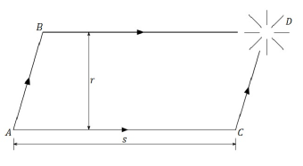
Figure 2: Experiment to detect gravity-induced quantum interference.

$$\phi_{\mathrm{ACD}}=mg\int_{C}^{D}z(t)dt.$$ (19)

Trajectory ABD gives in turn

$$\phi_{\mathrm{ABD}}=mg\int_{A}^{B}z(t)dt+mgr\int_{B}^{D}dt.$$ (20)

Bearing in mind that the neutron velocity is constant along the segment BD, we find that

$$\int_{B}^{D}dt\equiv\frac{s}{v}=\frac{sm\lambda}{2\pi}$$ (21)

where $\lambda=\frac{2\pi}{mv}$ is the de Broglie wavelength related to the neutron.

Therefore,

$$\Delta\phi=\phi_{\mathrm{ABD}}-\phi_{\mathrm{ACD}}=\frac{rsg\lambda m^{2}}{2\pi}.$$ (22)

So, we come to the conclusion that the phase shift obtained in COW experiment is dependent on the neutron mass. This landmark experiment reflects a divergence between the CEP and quantum mechanics. Note, however, that COW phase shift between the two neutron paths in which these particles are traveling at different heights in a gravitational field, depends on the (macroscopic) area of the quadrilateral formed by the neutron paths, being as a consequence a nonlocal effect. Thus, COW experiment does not violate the WEP.

We call attention to the fact that more recent and more accurate experiments have been performed since COW experiment (1975) in order to test the WEP on microscopic system via atom interferometry 30 ; 31 . Again, these experiments are in accord with the WEP (they are nonlocal) but disagree with the CEP.

III.2 Free fall in a constant gravitational field of a massive object described by its wave-function $\Psi$

Consider now the interesting but simple case of free fall in a constant gravitational field of a massive object quantum mechanical described by its wave function $\Psi$. We suppose that the wave-function is initially Gaussian.

In this case the Schrödinger equation must be satisfied with the Hamiltonian

$$H=\frac{p^{2}}{2m}+mgz.$$ (23)

The time of flight of the particle at hand can be computed from some initial position $z_{0}$ up to $z=0$, where the initial position is determined by the expectation value $z_{0}=\langle\Psi_{0}|z|\Psi_{0}\rangle$ of the position in the Gaussian initial state $\Psi_{0}$. Now, although the time of flight is statically distributed with the mean value agreeing with the classical universal value

$$T=\sqrt{\frac{2z_{0}}{g}},$$ (24)

the standard deviation of the measured values of the time of flight around $T$ depends on the mass of the particle

$$\sigma=\frac{2\pi}{\Delta_{0}mg},$$ (25)

being $\Delta_{0}$ the width of the initial Gaussian wave packet.

Therefore, we arrive at the conclusion that in this sense the quantum motion of the particle is non-universal since it depends on the value of its mass, which of course violates the CEP but not the WEP (the particle is an object extended in space).

IV Final remarks

Two semiclassical examples that violate the CEP but not the WEP in an external gravitational field, were discussed from a theoretical point of view: Greenberger gravitational Bohr atom and the deflection at the tree level of different quantum particles owed to an external weak higher-order gravitational field. In this latter case the bending is dependent on the spin and energy of the scattered particle. We analyzed also an experiment similar to the one just described where the external weak higher-order gravitational field is replaced by an external weak Einsteinian gravitational field which also violates the CEP but not the WEP.

Two quantum examples that also agree with the WEP but are not in accord with the CEP were analyzed afterwards: COW experiment and free fall in a constant gravitational field of a massive object described by its wave-function $\Psi$.

Now, among the four examples studied in this work only one is based on a experimental test: COW experiment. For this reason we shall elaborate a bit more on the aforementioned test. Although COW experiment was conducted in 1975, a more accurate version of the same was performed in 1997 32 , and its authors reported that in this experiment the gravitationally induced phase shift of the neutron was measured with a statistical uncertainty of order 1 part in 1000 in two different interferometers. A discrepancy between the theoretically predicted and experimentally measured value of the phase shift due to gravity was also observed at the 1$\%$ level. Extensions to the theoretical description of the shape of a neutron interferogram as function of the tilt in a gravitational field were discussed and compared with experiment as well. It is worthy of note that past experiments have verified the quantum-mechanical equivalence of gravitational and inertial masses to a precision of about 1$\%$.

We call attention to the fact that a phase shift of the form given in Eq. (22) would be predicted for a quantum -mechanical particle in the presence of any scalar potential; in our case is the Newtonian gravitational potential. In order to fully describe this effect we need only quantum mechanics and Newton theory. Therefore, no metric description of gravity is necessary. This phenomenon, of course, is unexplainable by classical Newtonian gravity. Undoubtedly, COW experiment represents the first evidence of gravity interacting in a truly quantum mechanical way. Nevertheless, from the viewpoint of quantum theory, this effect is well understood as a scalar Aharanov-Bohm effect and manifests similarly for electric charges in electric potentials 33 ; 34 .

We point out that the references 35 ; 36 ; 37 ; 38 may be helpful for those interested in investigations similar in a sense to those dealt with in the present work.

Last but not least, we would like to draw the reader’s attention to fact the examples discussed in this article seem to indicate that, at first sight, the only possibility of violating the WEP is through local experiments.

The authors are very grateful to FAPERJ and CNPq for their financial support.

Appendix A Unpolarized differential cross sections for tree-level scattering of different quantum particles by an external weak higher-order gravitational field

A.1 Spin-0 particles

The Lagrangian for a massive scalar field minimally coupled to gravity can be written as

$${\cal{L}}=\frac{\sqrt{-g}}{2}\Big{(}g^{\mu\nu}\partial_{\mu}\phi\partial_{\nu}\phi-m^{2}\phi^{2}\Big{)},$$ (26)

and leads to first order in $k$ to the following Lagrangian for the interaction of a scalar field with a weak gravitational field

$${\cal{L}}_{\mathrm{int}}=-\frac{\kappa}{2}h^{\mu\nu}\Big{[}\partial_{\mu}\phi\partial_{\nu}\phi-\frac{1}{2}\eta_{\mu\nu}\Big{(}\partial_{\alpha}\phi\partial^{\alpha}\phi-m^{2}\phi^{2}\Big{)}\Big{]}.$$

From the preceding Lagrangian we promptly obtain the vertex for the process depicted in figure A1

$$V({\bf p},{\bf q})=-\frac{\kappa}{2}h^{\mu\nu}_{\mathrm{ext}}({\bf{k}})\Big{[}p_{\mu}q_{\nu}+p_{\nu}q_{\mu}-\eta_{\mu\nu}(p\cdot q-m^{2})\Big{]},$$

where the external field is a weak higher-order gravitational field.

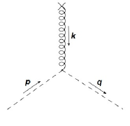
Figure 3: Feynman diagram for the interaction between a spin-0 particle and an external weak gravitational field.

Now, the differential cross section for the process above reads

$$\frac{d\sigma}{d\Omega}=\frac{{|\cal{M}|}^{2}}{(4\pi)^{2}},$$ (27)

where the Feynman amplitude ${\cal{M}}$ coincides with $V({\bf p},{\bf q})$.

Accordingly, the differential cross section for the tree-level scattering of a massive spin-0 particle by an external weak higher-derivative gravitational field assumes the form

$$\frac{d\sigma}{d\Omega}=\Bigg{[}\frac{GM}{\sin^{2}\frac{\theta}{2}}\Bigg{]}^{2}\Bigg{[}1+\frac{\lambda}{2}+\frac{\sin^{2}\frac{\theta}{2}-(3+2\lambda)}{3(1+\frac{1}{4}\lambda_{2}\csc^{2}\frac{\theta}{2})}+\frac{\frac{1}{2}\lambda-\sin^{2}\frac{\theta}{2}}{3(1+\frac{1}{4}\lambda_{0}\csc^{2}\frac{\theta}{2})}\Bigg{]}^{2},$$ (28)

where

$$\lambda\equiv\frac{m^{2}}{{\bf p}^{2}},\;\;\lambda_{2}\equiv\frac{M^{2}_{2}}{{\bf p}^{2}},\;\;\lambda_{0}\equiv\frac{M^{2}_{0}}{{\bf{p}}^{2}}.$$ (29)

Now, since $E^{2}={\bf p}^{2}(1+\lambda)$ where $E$ is the particle energy, $\lambda_{2}$ and $\lambda_{0}$ can be written as

$$\lambda_{2}=\frac{(1+\lambda)M^{2}_{2}}{E^{2}},\;\;\lambda_{0}=\frac{(1+\lambda)M^{2}_{0}}{E^{2}},$$ (30)

which clearly shows that all the parameters in Eq. (A.4) are energy dependent.

In the $m\rightarrow 0\;$ limit, we get the differential cross section for tree-level scattering of a massless spin-0 boson by an external weak higher-derivative gravitational field

$$\frac{d\sigma}{d\Omega}=\Bigg{[}\frac{GM}{\sin^{2}\frac{\theta}{2}}\Bigg{]}^{2}\Bigg{[}1+\frac{\sin^{2}\frac{\theta}{2}-3}{3(1+\frac{1}{4}\lambda_{2}\csc^{2}\frac{\theta}{2})}-\frac{\sin^{2}\frac{\theta}{2}}{{3(1+\frac{1}{4}\lambda_{0}\csc^{2}\frac{\theta}{2})}}\Bigg{]}^{2}.$$ (31)

Note that if $m=0$, $\lambda_{2}=\frac{M^{2}_{2}}{E^{2}}\;$ and $\lambda_{0}=\frac{M^{2}_{0}}{E^{2}}$. Here we are using the same symbols for denoting the parameters $\lambda_{2}$ and $\lambda_{0}$ as those utilized for the massive case since their meaning are quite clear from the context. Therefore, from now on these symbols will utilized for both massive and massless particles.

A.2 Spin-1/2 particles

As is well known, the gravitational Lagrangian for a massive fermion is given by 39

$${\cal{L}}=\sqrt{-g}\Bigg{[}\frac{i}{2}\Big{(}\bar{\psi}\gamma^{\mu}\overset{\rightarrow}{\nabla}_{\mu}\psi-\bar{\psi}\overset{\leftarrow}{\nabla}_{\mu}\gamma^{\mu}\psi\Big{)}-m\bar{\psi}\psi\Bigg{]},$$ (32)

with the notation

$$\gamma^{\mu}=\gamma^{p}e^{\mu}_{p},\;\overset{\rightarrow}{\nabla}_{\mu}\psi=\partial_{\mu}\psi+iw_{\mu}\psi,\;\bar{\psi}\overset{\leftarrow}{\nabla}_{\mu}=\partial_{\mu}\bar{\psi}-i\bar{\psi}w_{\mu}.$$

Here $e^{\nu}_{n}\equiv\eta_{mn}g^{\mu\nu}e^{m}_{\mu}(x)$ is a different type of vierbein where the $m$ index is lowered with the Minkowski metric $\eta_{nm}$, while the $\mu$ index is raised with $g^{\mu\nu}$; whereas the field connection $w_{\mu}(x)$ is expressed in terms of the tetrads as

$$w_{\mu}(x)=\frac{1}{4}\sigma^{mn}\Big{[}e^{\nu}_{m}\Big{(}\partial_{\mu}e_{n\nu}-\partial_{\nu}e_{n\mu}\Big{)}+\frac{1}{2}e^{\rho}_{m}e^{\sigma}_{n}\Big{(}\partial_{\sigma}e_{l\rho}-\partial_{\rho}e_{l\sigma}\Big{)}e^{l}_{\mu}-(m\leftrightarrow n)\Big{]},$$

where the Dirac matrices are denoted by $\gamma^{n}$, and $\sigma^{mn}=\frac{i}{2}[\gamma^{m},\gamma^{n}]$.

Keeping in mind that to order $k$ 40

$$e^{m}_{\mu}=\delta^{m}_{\mu}+\frac{\kappa}{2}h^{m}_{\mu}+{\cal{O}}(k^{2}),$$ (33)

we find that within this approximation the Lagrangian for the interaction of a fermion with a weak gravitational field has the form

$${\cal{L}}_{\mathrm{int}}= -\frac{\kappa}{2}h_{\mu\nu}\Bigg{\{}\frac{i}{2}\Big{[}\Big{(}\bar{\psi}\gamma^{\mu}\partial^{\nu}\psi-\partial^{\nu}\bar{\psi}\gamma^{\mu}\psi\Big{)}$$ (34)

$$-\eta^{\mu\nu}\Big{(}\bar{\psi}\gamma^{\alpha}\partial_{\alpha}\psi-\partial_{\alpha}\bar{\psi}\gamma^{\alpha}\psi\Big{)}\Big{]}+\eta^{\mu\nu}m\bar{\psi}\psi\Bigg{\}}.$$

It follows that the vertex for the process shown in figure A2 reads

$$V({\bf p},{\bf q})=\frac{\kappa}{8}h^{\mu\nu}_{\mathrm{ext}}({\bf{k}})\Bigg{[}2\eta_{\mu\nu}\Big{(}\not{p}+\not{q}-2m\Big{)}-\gamma_{\mu}(p+q)_{\nu}-(p+q)_{\mu}\gamma_{\nu}\Bigg{]},$$ (35)

where $h^{\mu\nu}_{\mathrm{ext}}({\bf k})$ is given by (7).

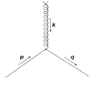
Figure 4: Diagram for the interaction of a fermion with an external weak gravitational field.

The unpolarized differential cross section for the process at hand, in turn, is given by

$$\frac{d\sigma}{d\Omega}=\frac{(2m)^{2}}{(4\pi)^{2}}\frac{1}{2}\sum_{r^{\prime},r}\Big{|}{\cal{M}}_{r^{\prime},r}\Big{|}^{2},$$ (36)

where

$${\cal{M}}_{r^{\prime},r}=\bar{u}_{r^{\prime}}({\bf q})V({\bf p},{\bf q})u_{r}{(\bf p)}.$$

Taking the relation

$$\sum_{r=1}^{2}u_{r}({\bf p})\bar{u}_{r}({\bf p})=\frac{\not{p}+m}{2m}$$ (37)

into account, we find that the unpolarized differential cross section for the scattering of a massive fermion by an external weak higher-order gravitational field reads

$$\frac{d\sigma}{d\Omega}= \Bigg{(}\frac{GM}{\sin^{2}\frac{\theta}{2}}\Bigg{)}^{2}\sum_{n=0}^{2}\Bigg{[}\frac{E_{n}(\lambda)^{n}}{4}+\frac{A_{n}(\lambda)^{n}}{9(4+\lambda_{2}\csc^{2}\frac{\theta}{2})^{2}}$$

$$+\frac{B_{n}(\lambda)^{n}}{9(4+\lambda_{0}\csc^{2}\frac{\theta}{2})^{2}}+\frac{C_{n}(\lambda)^{n}}{9(4+\lambda_{2}\csc^{2}\frac{\theta}{2})(4+\lambda_{0}\csc^{2}\frac{\theta}{2})}\Bigg{]},$$

where

$$E_{0}=4\cos^{2}\frac{\theta}{2},\;\;E_{1}=3\cos^{2}\frac{\theta}{2}+1,\;\;E_{2}=1;$$

$$A_{0}=-(72\cos^{2}\frac{\theta}{2})\lambda_{2}\csc^{2}\frac{\theta}{2}-144\cos^{2}\frac{\theta}{2},$$

$$A_{1}=-(60\cos^{2}\frac{\theta}{2})\lambda_{2}\csc^{2}\frac{\theta}{2}-24\lambda_{2}\csc^{2}\frac{\theta}{2}-112\cos^{2}\frac{\theta}{2}-32,$$

$$A_{2}=-24\lambda_{2}\csc^{2}\frac{\theta}{2}-32;$$

$$B_{0}=0,$$

$$B_{1}=(6\cos^{2}\frac{\theta}{2})\lambda_{0}\csc^{2}\frac{\theta}{2}+6\lambda_{0}\csc^{2}\frac{\theta}{2}\ +20\cos^{2}\frac{\theta}{2}+28,$$

$$B_{2}=6\lambda_{0}\csc^{2}\frac{\theta}{2}+28;$$

$$C_{0}=0,\;\;C_{1}=-16\cos^{2}\frac{\theta}{2}-32,\;\;C_{2}=-32.$$

In the $m\rightarrow 0$ limit, we obtain the differential cross section for a massless fermion

$$\frac{d\sigma}{d\Omega}=\Bigg{(}\frac{GM}{\sin^{2}\frac{\theta}{2}}\Bigg{)}^{2}\cos^{2}\frac{\theta}{2}\Bigg{[}1-\frac{1}{1+\frac{1}{4}\lambda_{2}\csc^{2}\frac{\theta}{2}}\Bigg{]}^{2}.$$ (38)

A.3 Spin-1 particles

The gravitational Lagrangian for a massive photon can be written as

$${\cal{L}}=\sqrt{-g}\Bigg{[}-\frac{1}{4}g^{\mu\alpha}g^{\nu\beta}F_{\mu\nu}F_{\alpha\beta}+\frac{m^{2}}{2}g^{\mu\nu}A_{\mu}A_{\nu}\Bigg{]},$$ (39)

from which we trivially obtain the Lagrangian for the interaction of a massive photon with a weak gravitational field

$${\cal{L}_{\mathrm{int}}}=-\frac{\kappa}{2}h^{\mu\nu}\Big{[}\frac{1}{4}\eta_{\mu\nu}F^{2}_{\alpha\beta}-F_{\mu}^{\;\alpha}F_{\nu\alpha}+m^{2}\Big{(}A_{\mu}A_{\nu}-\frac{1}{2}\eta_{\mu\nu}A^{2}_{\alpha}\Big{)}\Big{]}.$$

Accordingly, the vertex for process represented in figure A3 is given by

$$V_{\alpha\beta}({\bf p},{\bf q})= -\frac{\kappa}{2}h^{\mu\nu}_{\mathrm{ext}}({\bf{k}})\Bigg{[}\Big{(}\eta_{\alpha\beta}\eta_{\mu\nu}-\eta_{\alpha\mu}\eta_{\beta\nu}-\eta_{\alpha\nu}\eta_{\beta\mu}\Big{)}$$

$$\Big{(}p\cdot q-m^{2}\Big{)}-\eta_{\alpha\beta}p_{\nu}q_{\mu}+\eta_{\mu\beta}p_{\nu}q_{\alpha}-\eta_{\mu\nu}p_{\beta}q_{\alpha}$$

$$+\eta_{\alpha\nu}p_{\beta}q_{\mu}+\eta_{\beta\nu}p_{\alpha}q_{\mu}-\eta_{\mu\nu}p_{\alpha}q_{\beta}+\eta_{\alpha\mu}p_{\nu}q_{\beta}\Bigg{]},$$

where the external field is a weak higher-order gravitational fied.

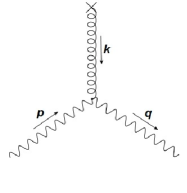
Figure 5: Diagram for the interaction between a photon and an external weak gravitational field.

Therefore, the unpolarized differential cross section for the process above can be written as

$$\frac{d\sigma}{d\Omega}=\frac{1}{(4\pi)^{2}}\frac{1}{3}\sum_{r^{\prime},r}\Big{|}{\cal{M}}_{r^{\prime},r}\Big{|}^{2},$$ (40)

where

$${\cal{M}}_{r^{\prime},r}=\epsilon^{\alpha}_{r^{\prime}}({\bf q})V_{\alpha\beta}({\bf p},{\bf q})\epsilon^{\beta}_{r}({\bf p}).$$ (41)

Here $\epsilon^{\beta}_{r}({\bf p})$ and $\epsilon^{\alpha}_{r^{\prime}}({\bf q})$ are respectively the ingoing and outgoing photon polarizations.

Now, bearing in mind that

$$\sum_{r=1}^{3}\epsilon^{\mu}_{r}({\bf p})\epsilon^{\nu}_{r}({\bf p})=-\eta^{\mu\nu}+\frac{p^{\mu}p^{\nu}}{m^{2}},$$ (42)

we come to the conclusion that

$$\frac{d\sigma}{d\Omega}= \Bigg{(}\frac{GM}{\sin^{2}\frac{\theta}{2}}\Bigg{)}^{2}\sum_{n=0}^{2}\Bigg{[}\frac{E^{\prime}_{n}(\lambda)^{n}}{12}+\frac{A^{\prime}_{n}(\lambda)^{n}}{27(4+\lambda_{2}csc^{2}\frac{\theta}{2})^{2}}$$

$$+\frac{B^{\prime}_{n}(\lambda)^{n}}{27(4+\lambda_{0}csc^{2}\frac{\theta}{2})^{2}}+\frac{C^{\prime}_{n}(\lambda)^{n}}{27(4+\lambda_{2}csc^{2}\frac{\theta}{2})(4+\lambda_{0}csc^{2}\frac{\theta}{2})}\Bigg{]},$$

where

$$E^{\prime}_{0}=4+8\cos^{4}\frac{\theta}{2},\;E^{\prime}_{1}=-4+16\cos^{2}\frac{\theta}{2},\;E^{\prime}_{2}=3;$$

$$A^{\prime}_{0}= -128-32\cos^{2}\frac{\theta}{2}-272\cos^{4}\frac{\theta}{2}+168\lambda_{2}$$

$$+144\lambda_{2}\cos^{2}\frac{\theta}{2}-216\lambda_{2}\csc^{2}\frac{\theta}{2},$$

$$A^{\prime}_{1}=160-592\cos^{2}\frac{\theta}{2}+324\lambda_{2}-252\lambda_{2}\csc^{2}\frac{\theta}{2},$$

$$A^{\prime}_{2}=-96-72\lambda_{2}\csc^{2}\frac{\theta}{2};$$

$$B^{\prime}_{0}=-80+64\cos^{2}\frac{\theta}{2}+16\cos^{4}\frac{\theta}{2}-24\lambda_{0},$$

$$B^{\prime}_{1}=16+128\cos^{2}\frac{\theta}{2}-36\lambda_{0}+36\lambda_{0}\csc^{2}\frac{\theta}{2},$$

$$B^{\prime}_{2}=84+18\lambda_{0}csc^{2}\frac{\theta}{2};$$

$$C^{\prime}_{0}=64-32\cos^{2}\frac{\theta}{2}-32\cos^{4}\frac{\theta}{2},$$

$$C^{\prime}_{1}=-32-112\cos^{2}\frac{\theta}{2},\;\;C^{\prime}_{2}=-96.$$

On the other hand, the gravitational Lagrangian for a massless photon has the form

$${\cal L}=\sqrt{-g}\Big{(}\frac{1}{4}g^{\mu\alpha}g^{\nu\beta}F_{\mu\nu}F_{\alpha\beta}\Big{)},$$ (43)

and from it we find the Lagrangian for the interaction between a massless photon and a weak gravitational

$${\cal{L}}_{\mathrm{int}}=-\frac{\kappa}{2}h^{\mu\nu}\Bigg{(}\frac{1}{4}\eta_{\mu\nu}F^{2}_{\alpha\beta}-F^{\;\alpha}_{\mu}F_{\nu\alpha}\Bigg{)}.$$ (44)

It follows then that the vertex for the interaction of a massless photon with an external weak higher-order gravitational field reads

$$V_{\alpha\beta}({\bf p},{\bf q})= -\frac{\kappa}{2}h^{\mu\nu}_{\mathrm{ext}}({\bf{k}})\Bigg{[}\Big{(}\eta_{\alpha\beta}\eta_{\mu\nu}-\eta_{\alpha\mu}\eta_{\beta\nu}-\eta_{\alpha\nu}\eta_{\beta\mu}\Big{)}p\cdot q$$

$$-\eta_{\alpha\beta}p_{\nu}q_{\mu}+\eta_{\mu\beta}p_{\nu}q_{\alpha}-\eta_{\mu\nu}p_{\beta}q_{\alpha}+\eta_{\alpha\nu}p_{\beta}q_{\mu}$$

$$+\eta_{\beta\nu}p_{\alpha}q_{\mu}-\eta_{\mu\nu}p_{\alpha}q_{\beta}+\eta_{\alpha\mu}p_{\nu}q_{\beta}\Bigg{]}.$$

Now, the differential cross section for the process under discussion can be written as

$$\frac{d\sigma}{d\Omega}=\frac{1}{(4\pi)^{2}}\frac{1}{2}\sum_{r^{\prime},r}\Big{|}{\cal{M}}_{r^{\prime},r}\Big{|}^{2},$$ (45)

where

$${\cal{M}}_{r^{\prime},r}=\epsilon^{\alpha}_{r^{\prime}}({\bf q})V_{\alpha\beta}({\bf p},{\bf q})\epsilon^{\beta}_{r}({\bf p}).$$ (46)

Keeping in mind that

$$\sum_{r=1}^{2}\epsilon^{\mu}_{r}({\bf p})\epsilon^{\nu}_{r}({\bf p})=-\eta_{\mu\nu}-\frac{1}{(p\cdot n)^{2}}\Big{[}p^{\mu}p^{\nu}-p\cdot n\Big{(}p^{\mu}n^{\nu}+p^{\nu}n^{\mu}\Big{)}\Big{]},$$

where $n^{2}=1$, we arrive at the conclusion that

$$\frac{d\sigma}{d\Omega}=\Bigg{(}\frac{GM}{\sin^{2}\frac{\theta}{2}}\Bigg{)}^{2}\cos^{4}\frac{\theta}{2}\Bigg{(}1-\frac{1}{1+\frac{1}{4}\lambda_{2}\csc^{2}\frac{\theta}{2}}\Bigg{)}^{2}.$$

References

References

• (1) D. Greenberger, Ann. Phys. (NY) 47, 116 (1968).
• (2) R. Colella, A. Overhauser, and S. Werner, Phys. Rev. Lett. 34, 1472 (1975).
• (3) R. Aldrovandi, J. Pereira, and K. Vu, AIP Conf. Proc. 810, 217 (2006).
• (4) R. Aldrovandi, J. Pereira, and K. Vu, AIP Conf. Proc. 861, 277 (2006).
• (5) N. Kajuri, Phys. Rev. D 94, 084007 (2016).
• (6) C. Will, arXiv: 1403. 7377v1 [gr-qc].
• (7) K. Thorne, D. Lee, and A. Lightman, Phys. Rev. D 7, 3563 (1973).
• (8) H. Ohanian, Phys. Rev. D 10, 2041 (1974).
• (9) W.-T. Ni, Phys. Rev. Lett. 38, 301 (1977).
• (10) A. Coley, Phys. Rev. Lett. 49, 853 (1982).
• (11) A. Accioly, U. Wichoski, and N. Bertarello, Braz. J. Phys. 23, 392 (1993).
• (12) M. Haugan, Ann. Phys. (N.Y.) 118, 156 (1979).
• (13) A. Lightman and D. Lee, Phys. Rev. D 8, 364 (1973).
• (14) K. Stelle, Phys. Rev. D 16, 953 (1977).
• (15) A. Accioly, G. Correia, G. P. Brito, J. de Almeida, and W. Herdy, Mod. Phys. Lett. A 32, 1750048 (2017).
• (16) A. Accioly, J. de Almeida, G. P. Brito, and G. Correia, Phys. Rev. D 95, 084007 (2017).
• (17) I. L. Shapiro, A. Pelinson, and F. Salles, Mod. Phys. Lett. A 29, 1430034 (2014).
• (18) T. Sotiriou and V. Faraoni, Rev. Mod. Phys. 82, 451 (2010).
• (19) A. Accioly, J. Helayël-Neto, B. Giacchini, and W. Herdy, Phys. Rev. D 91, 125009 (2015).
• (20) P. Teyssandier, Classical Quantum Gravity 6, 219 (1989).
• (21) A. Accioly, A. Azeredo, H. Mukai, and E. de Rey Neto, Prog. Theor. Phys. 104, 103 (2000).
• (22) A. Accioly and S. Ragusa, Classical Quantum Gravity 19, 5429 (2002); (E) 20, 4963 (2003).
• (23) A. Accioly, J. Helayël-Neto, and E. Scatena, Phys. Lett. A 374, 3806 (2010).
• (24) A. Accioly, J. Helayël-Neto, E. Scatena, R. Turcati, and J. Morais, Classical Quantum Gravity 27, 205010 (2010).
• (25) A. Accioly, J. Helayël-Neto, and E. Scatena, Phys. Rev. D 82, 065026 (2010).
• (26) R. Aldrovandi, J. Pereira, and K. Vu, Classical Quantum Gravity 21, 51 (2004).
• (27) T. Wu and C. Yang, Phys. Rev. D 12, 3845 (1975).
• (28) R. Aldrovandi, J. Pereira, and K. Vu, Gen. Relat. Grav. 36, 101 (2004).
• (29) R. Aldrovandi and J. Pereira, Teleparallel Gravity, Fundamental Theories of Physics vol 173, Springer (2013).
• (30) A. Peters, K. Chung, and S. Chu, Nature 400, 849 (1999).
• (31) S. Merlet, Q. Bodart, N. Malossi, A. Landragin, F. Dos Santos, O. Gitlein, and L. Timmen, Metrologia 47, L9 (2010).
• (32) K. Littrell, B. Allman, and S. Werner, Phys. Rev A 56 , 1767 (1997).
• (33) M. Zych, F. Costa, I. Pikovski, and C̆. Brukner, Nature Commun. 2, 505, (2011).
• (34) B. Allman, W.-T. Lee, O. Motrunich, and S. Werner, Phys. Rev. A 60, 4272 (1999).
• (35) G. Rosi, G. D’Amico, L. Cacciapuoti, F. Sorrentino, M. Prevedelli, M. Zych, C̆. Brukner, and G. Timo, arXiv:1704.02296v2 [physics.atom-ph].
• (36) M. Zich and C̆. Brukner, arXiv:1502.00971v1 [gr-qc].
• (37) P. Orlando, R. Mann, K. Modi, and F. Pollock, arXiv:1511.02943v1 [quant-ph].
• (38) P. Orlando, F. Pollock, and K. Modi, arXiv:1610.02141v1 [quant-ph].
• (39) S. Choi, J. Shim, and H. Song, Phys. Rev. D 51, 2751 (1955).
• (40) R. Woodard, Phys. Lett. 148B, 440 (1984); H. Cho and K. Ng, Phys. Rev. D 47, 1692 (1993).