Continuous-Variable Entanglement Test in Driven Quantum Contacts

Abstract

The standard entanglement test using the Clauser-Horne-Shimony-Holt inequality is known to fail in mesoscopic junctions at finite temperatures. Since this is due to the bidirectional particle flow, a similar failure is expected to occur in an ac-driven contact. We develop a continuous-variable entanglement test suitable for electrons and holes that are created by the ac drive. At low enough temperatures the generalized Bell inequality is violated in junctions with low conductance or small number of transport channels and with ac voltages which create few electron-hole pairs per cycle. Our ac-entanglement test depends on the total number of electron-hole pairs and on the distribution of probabilities of pair creations similar to the Fano factor.

Quantum mechanics in fact is a nonlocal theory. In 1935 Einstein, Podolsky, and Rosen put forward the EPR paradox Einstein et al. (1935) to question the completeness of quantum mechanics which disobeys, in their view apparent, the principle of local realism. They argued that quantum mechanics should be completed with some hidden variables. In 1964 Bell derived an inequality Bell (1964) to actually test the principle of local realism. Remarkably, he found that in some cases the physical results based on the principle of local realism are inconsistent with the predictions of quantum mechanics. In later years, the experiments on quantum entanglement Freedman and Clauser (1972); *aspect_experimental_1981; *aspect_experimental_1982; *rarity_experimental_1990; *rowe_experimental_2001; *weihs_violation_1998 proved the existence of nonlocality, including the recent loophole-free or human-choice-driven tests Hensen et al. (2015); Giustina et al. (2015); Shalm et al. (2015); Collaboration (2018). Besides their fundamental importance, quantum entanglement and nonlocality have attracted a lot of attention over the past two decades in the context of quantum computation Steane (1998), teleportation Bennett et al. (1993); Boschi et al. (1998), and cryptography Gisin et al. (2002). While most of the tests are performed using quantum optics, it still remains a challenge to detect entanglement within the Fermi sea in mesoscopic systems Burkard et al. (2000); Loss and Sukhorukov (2000); Recher et al. (2001); Bena et al. (2002); Samuelsson et al. (2003, 2004); Beenakker et al. (2003); *beenakker_optimal_2005; Samuelsson et al. (2009); Klich and Levitov (2009). Some of these concepts have even been tested experimentally Hofstetter et al. (2009); Gabor et al. (2009); Herrmann et al. (2010); Hofstetter et al. (2011); Simmons et al. (2011); Das et al. (2012); Schindele et al. (2012); Fülöp et al. (2015); Gramich et al. (2017).

The most common way to detect the entanglement is to test for the violation of the Clauser-Horne-Shimony-Holt (CHSH) inequality Clauser et al. (1969).

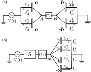
Figure 1: Setups for the generalized ac Bell test: (a) normal junction with transmission eigenvalues $\{T_{n}\}$ and (b) superconductor – normal-metal beam splitter. In both cases, the test observables are the differences between the numbers of spin-up and spin-down particles along directions $\pm\bm{a}$ and $\pm\bm{b}$ detected in the leads A (Alice) and B (Bob).

In mesoscopic junctions as shown in Fig. 1, the CHSH inequality reads $|C(\bm{a},\bm{b})+C(\bm{a},\bm{b}^{\prime})+C(\bm{a}^{\prime},\bm{b})-C(\bm{a}^{\prime},\bm{b}^{\prime})|\leq 2$ where $C(\bm{n}_{A},\bm{n}_{B})=\langle(N_{A}^{\uparrow}-N_{A}^{\downarrow})(N_{B}^{\uparrow}-N_{B}^{\downarrow})\rangle/\langle(N_{A}^{\uparrow}+N_{A}^{\downarrow})(N_{B}^{\uparrow}+N_{B}^{\downarrow})\rangle$ are the spin correlators and $N_{j}^{\sigma}$ are the numbers of quasiparticles with spin projections $\sigma=\uparrow,\downarrow$ in direction $\bm{n}_{j}$ detected in the lead $j=A,B$. Assuming 100% efficient detectors, the spin correlators can be expressed in terms of the average current $I_{0}$ and current noise power $S_{0}$ Chtchelkatchev et al. (2002), $C(\bm{n}_{A},\bm{n}_{B})=-\bm{n}_{A}\cdot\bm{n}_{B}S_{0}/(S_{0}+2\tau I_{0}^{2})$, where $\tau$ is the measurement time. What is peculiar about this result is that it reduces to $C(\bm{n}_{A},\bm{n}_{B})=-\bm{n}_{A}\cdot\bm{n}_{B}$ in an ac driven system with no dc bias ($I_{0}=0$). In that case, the CHSH inequality can always be maximally violated with the left-hand side equal to $2\sqrt{2}$ if the angles between the spin polarization directions in the leads are chosen as $\theta_{\bm{a}\bm{b}}=\theta_{\bm{a}^{\prime}\bm{b}}=\theta_{\bm{a}\bm{b}^{\prime}}=\pi/4$ and $\theta_{\bm{a}^{\prime}\bm{b}^{\prime}}=3\pi/4$. However, this violation does not mean entanglement because it cannot single out the entangled pair if there are many entangled pairs. In addition, it is implausible that the violation is independent of the amplitude and the frequency of the ac voltage and even the shape of the drive. The reason why the CHSH inequality fails to reveal the entanglement is because it requires unidirectional particle flow in the leads, a condition which is not satisfied when we apply ac voltage to the system. Indeed, ac drive leads to fluctuations with $|N_{j}^{\uparrow}-N_{j}^{\downarrow}|>|N_{j}^{\uparrow}+N_{j}^{\downarrow}|$ which are forbidden in the Bell test Chtchelkatchev et al. (2002). The same problem occurs in a dc biased junction at finite temperatures Hannes and Titov (2008). To detect entanglement in an ac driven junction, a generalized Bell test is needed which is free from this restriction.

In this Letter, we study two different setups for a generalized Bell test in ac driven systems at low temperatures. The setup shown in Fig. 1(a) is a normal junction with transmission eigenvalues $\{T_{n}\}$ biased by the periodic ac voltage $V(t)$ with frequency $\omega$ and zero average. The second setup, shown in Fig. 1(b), is an ac-driven superconductor (S) – normal-metal (N) beam splitter which emits entangled pairs of electrons or holes. In both cases, the spin-polarized particles along directions $\pm\bm{a}$ and $\pm\bm{b}$ are detected in the leads A (Alice) and B (Bob). The test observables are the differences between the numbers of spin-up and spin-down particles $\hat{A}\equiv\hat{N}_{A}^{\uparrow}-\hat{N}_{A}^{\downarrow}=\int dt(\hat{I}_{A}^{\uparrow}-\hat{I}_{A}^{\downarrow})/e$ and $\hat{B}\equiv\hat{N}_{B}^{\uparrow}-\hat{N}_{B}^{\downarrow}=\int dt(\hat{I}_{B}^{\uparrow}-\hat{I}_{B}^{\downarrow})/e$. In contrast to the dc bias which at zero temperature leads to unidirectional electron transport Bednorz and Belzig (2011); Lorenzo and Nazarov (2005), the ac drive generates electron-hole pairs in the junction Vanević et al. (2007); *vanevic_elementary_2008; Belzig and Vanević (2016); Vanević and Belzig (2012); Vanević et al. (2016). The particle flow in the leads is therefore bidirectional which renders the standard Bell test inapplicable. In this Letter, we derive a generalized Bell inequality for the proposed setups,

$$\sqrt{3}(2-\sqrt{2})/4\leq\sqrt{1-\langle A^{2}\rangle/\langle A^{4}\rangle},$$ (1)

whose violation implies the presence of entangled particles in the system. Since Eq. (1) requires access to the fourth-order spin current correlations, we anticipate the use of low-Ohmic spin-polarized contacts which convert the spin into charge currents or testing the spin-dependent chemical potentials using ferromagnetic tunnel junctions Das et al. (2012); Arakawa et al. (2015). Expressing the moments $\langle A^{2}\rangle$ and $\langle A^{4}\rangle$ in terms of transmission eigenvalues and properties of the drive, we find

$$\frac{\sqrt{2}-1}{4}\leq\sqrt{\frac{X_{i}}{1+6X_{i}}}.$$ (2)

Here, $X_{i}=\sum_{n,k}P_{n,k}^{(i)}-\sum_{n,k}P_{n,k}^{(i)2}/\sum_{n,k}P_{n,k}^{(i)}$ where $i=1$ ($2$) stands for the normal (superconducting) junction shown in Fig. 1. The probabilities $P_{n,k}^{(1)}=p_{k}T_{n}R_{n}$ and $P_{n,k}^{(2)}=p_{k}R_{n}^{A}/4$, where $R_{n}=1-T_{n}$ and $R_{n}^{A}=T_{n}^{2}/(2-T_{n})^{2}$ are normal and Andreev reflection coefficients; $p_{k}$ ($k=1,2,\ldots$) are the probabilities of electron-hole pair creations which depend on the details of the drive Vanević et al. (2007); *vanevic_elementary_2008; Vanević and Belzig (2012). For the harmonic drive, the dependence of the $p_{k}$ on the drive amplitude is shown in Fig. 2 (a).

To derive Eqs. (1) and (2), we first obtain the statistics of $\hat{A}$ and $\hat{B}$ in the junctions at hand. The statistics is computed by using the circuit theory of quantum transport. We assign the counting fields $\chi_{A}^{\sigma}$ and $\chi_{B}^{\sigma}$ ($\sigma=\uparrow,\downarrow$) to the spin-polarized leads of Alice and Bob, see Fig. 1. Since we are only interested in the differences between the numbers of spin-up and spin-down particles, we can set $\chi_{A}^{\uparrow}=-\chi_{A}^{\downarrow}=\chi_{A}$ and $\chi_{B}^{\uparrow}=-\chi_{B}^{\downarrow}=\chi_{B}$, where $\chi_{A}$ and $\chi_{B}$ are the counting fields which determine the statistics of $\hat{A}$ and $\hat{B}$. For the cumulant generating functions ${\cal S}_{1}$ and ${\cal S}_{2}$ of the normal and the superconducting junction shown in Fig. 1 we find sup

$${\cal S}_{i}(\chi_{A},\chi_{B})=M\sum_{n,k}\ln\bigg{(}1+P_{n,k}^{(i)}\\ \times\sum_{\alpha,\beta=\pm 1}\frac{1+\alpha\beta\bm{a}\cdot\bm{b}}{2}(e^{i\alpha\chi_{A}-i\beta\chi_{B}}-1)\bigg{)}.$$ (3)

Here, $M=\tau\omega/\pi$ and we assumed low temperature $T_{e}\ll\omega$ and $\omega\ll\Delta$ in the superconducting case, which is in the experimentally accessible range. We later discuss the effect of finite temperature along the lines of electron-hole pair creation in Ref. Vanević et al. (2007). In the remainder of the Letter we set $M=1$ which is the optimal value for the Bell test. Indeed, as the measuring time $\tau$ is increased the number of particles detected also increases which will destroy the entanglement test. Experimentally, the inverse measuring time $1/\tau$ is related to the bandwidth of the detection setup. Hence, $M=1$ can be achieved by measuring the cumulants of $\hat{A}$ and $\hat{B}$ in a large bandwidth $1/\tau\sim\omega$, which is equivalent to dividing the result by $M$ and justifies the setting of $M=1$ in the following.

Next we apply the generalized Bell inequality Bednorz and Belzig (2011)

$$|\langle AB(A^{2}+B^{2})\rangle+\langle A^{\prime}B(A^{\prime 2}+B^{2})\rangle+\langle AB^{\prime}(A^{2}+B^{\prime 2})\rangle\\ -\langle A^{\prime}B^{\prime}(A^{\prime 2}+B^{\prime 2})\rangle|\leq\langle A^{4}\rangle+\langle A^{\prime 4}\rangle+\langle B^{4}\rangle+\langle B^{\prime 4}\rangle\\ +\frac{1}{2}\sideset{}{{}^{*}}{\sum}_{C,D,E}\sqrt{\sqrt{\langle C^{4}\rangle}\sqrt{\langle D^{4}\rangle}\langle(D^{2}-E^{2})^{2}\rangle}.$$ (4)

Here, the summation is taken over $C,D,E\in\{A,A^{\prime},B,B^{\prime}\}$ and ^∗ denotes the restriction $D\neq C$ and $E\neq C,D,D^{\prime}$. Importantly, inequality in Eq. (4) does not require a quantized measurement or unidirectional particle flow and also does not pose restrictions on the possible values of the observables $A,A^{\prime},B,B^{\prime}$. As with any Bell test, the symbol ^′ in Eq. (4) denotes two different settings of the Alice and Bob measuring apparatus. In this case these are the two choices of spin-polarization directions $\bm{a}$, $\bm{a}^{\prime}$ for Alice and $\bm{b}$, $\bm{b}^{\prime}$ for Bob. The cumulants of $\hat{A}$ and $\hat{B}$ are obtained by taking derivatives of the cumulant generating function in Eq. (3) with respect to the counting fields. From the cumulants we can find the moments which appear in Eq. (4). We obtain the following relations which are valid for both setups: $\langle A^{(\prime)}\rangle=\langle B^{(\prime)}\rangle=0$, $\langle A^{(\prime)4}\rangle=\langle B^{(\prime)4}\rangle$, $\langle A^{(\prime)3}B^{(\prime)}\rangle=\langle A^{(\prime)}B^{(\prime)3}\rangle=-\bm{a}^{(\prime)}\cdot\bm{b}^{(\prime)}\langle A^{4}\rangle$, $\langle A^{(\prime)2}B^{(\prime)2}\rangle=(1/3)[1+2(\bm{a}^{(\prime)}\cdot\bm{b}^{(\prime)})^{2}]\langle A^{4}\rangle+(2/3)[1-(\bm{a}^{(\prime)}\cdot\bm{b}^{(\prime)})^{2}]\langle A^{2}\rangle$. Substituting these relations in Eq. (4), we obtain $|\mathcal{B}(\bm{a},\bm{b},\bm{a}^{\prime},\bm{b}^{\prime})|\leq 2+(2/\sqrt{3})\sqrt{1-\langle A^{2}\rangle/\langle A^{4}\rangle}\sum_{\bm{c},\bm{d}}\sqrt{1-(\bm{c}\cdot\bm{d})^{2}}$ where $\bm{c}\in\{\bm{a},\bm{a}^{\prime}\}$, $\bm{d}\in\{\bm{b},\bm{b}^{\prime}\}$, and $\mathcal{B}(\bm{a},\bm{b},\bm{a}^{\prime},\bm{b}^{\prime})=\bm{a}\cdot\bm{b}+\bm{a}^{\prime}\cdot\bm{b}+\bm{a}\cdot\bm{b}^{\prime}-\bm{a}^{\prime}\cdot\bm{b}^{\prime}$. Choosing the angles between spin-polarization directions $\theta_{\bm{a}\bm{b}}=\theta_{\bm{a}^{\prime}\bm{b}}=\theta_{\bm{a}\bm{b}^{\prime}}=\pi/4$ and $\theta_{\bm{a}^{\prime}\bm{b}^{\prime}}=3\pi/4$ such that $|\mathcal{B}|$ is maximal, the generalized Bell inequality reduces to Eq. (1). Finally, after computing the moments $\langle A^{2}\rangle=\partial^{2}_{i\chi_{A}}{\cal S}|_{\chi=0}$ and $\langle A^{4}\rangle=3\langle A^{2}\rangle^{2}+\partial^{4}_{i\chi_{A}}{\cal S}|_{\chi=0}$ we recover Eq. (2).

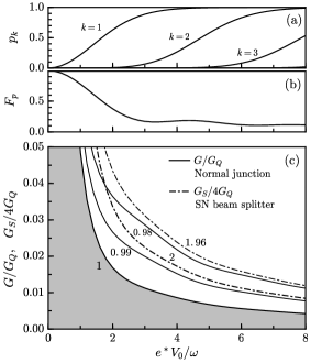
Figure 2: (a) Probabilities of electron-hole pair creations $p_{k}$ and (b) parameter $F_{p}=\sum_{k}p_{k}(1-p_{k})/\sum_{k}p_{k}$ as a function of the amplitude $V_{0}$ for harmonic drive $V(t)=V_{0}\cos(\omega t)$. (c) Test of a generalized Bell inequality: Normal junction [solid lines, see Eq. (5) and Fig. 1(a)] and SN beam splitter geometry [dash-dotted lines, see Eq. (6) and Fig. 1(b)]. The generalized Bell inequality is violated for junction conductances and applied voltages that are below the lines shown in (c). Fano factors $F=1$, $0.99$, $0.98$ ($F_{S}=2$, $1.96$) for the normal (superconducting) junction are shown in the plot. The effective charge is $e^{*}=e$ for the normal and $e^{*}=2e$ for the SN junction.

Equations (1) and (2) represent a generalized Bell test suitable for driven systems shown in Fig. 1, where the particle flow in the leads is bidirectional due to the presence of electron-hole pairs created by the drive. When the number of transport channels is large, Eq. (2) reduces to $(\sqrt{2}-1)/4\leq 1/\sqrt{6}$ which is not violated, as one might expect. The same is true when many electron-hole pairs are created in the system ($p_{k}=1$ for $k=1,\ldots,N_{eh}$; $N_{eh}\gg 1$). To violate Eq. (2), the contribution of an entangled pair has to be singled out from the rest. This is achieved in a junction with low conductance or small number of transport channels and with few particles created per voltage cycle. In the low conductance limit, Eq. (2) reduces to $(\sqrt{2}-1)/4\leq\beta_{i}$ where to lowest order in $1-F$($1-F_{S}/2$)

$$\beta_{1}^{2}=\frac{G}{G_{Q}}\sum_{k}p_{k}-(1-F_{p})(1-F)$$ (5)

and

$$\beta_{2}^{2}=\frac{1}{4}\left(\frac{G_{S}}{2G_{Q}}\sum_{k}p_{k}-(1-F_{p})(1-F_{S}/2)\right)$$ (6)

for the normal junction and the SN beam splitter, respectively. Here, $G=G_{Q}\sum_{n}T_{n}$ ($G_{S}=2G_{Q}\sum_{n}R^{A}_{n}$) and $F=\sum_{n}T_{n}R_{n}/\sum_{n}T_{n}$ ($F_{S}=2\sum_{n}R^{A}_{n}(1-R^{A}_{n})/\sum_{n}R^{A}_{n}$) are the conductance and the Fano factor of the normal (superconducting) junction, and $G_{Q}=e^{2}/\pi$. The distribution of probabilities of electron-hole pair creations is characterized by $F_{p}=\sum_{k}p_{k}(1-p_{k})/\sum_{k}p_{k}$, in analogy with the Fano factor for the transmission eigenvalues. The Bell test is analyzed in Fig. 2 as a function of the junction conductance, the amplitude of applied voltage, and different Fano factors that are close to the tunnel limit. We find that small deviations from the Poissonian statistics, that is, the presence of open channels, helps in violating the generalized Bell inequality. We note, that the Bell test also depends on the details of the drive through the probabilities $p_{k}$ and distribution $F_{p}$ of electron-hole pair creations, which we will discuss later. It is also interesting by how much the inequality is violated for a given set of parameters. This extent of the Bell inequality violation is shown in Fig. 3 for the harmonic drive. As we see, small amplitudes $V_{0}$ are in general favorable. In practice, a finite temperature sets an upper limit on $V_{0}$ for the Bell inequality violation, which we will discuss in Fig. 5. As regards the efficiency of the spin filters, we find that imperfect spin polarization decreases the possibility to violate our generalized Bell inequality sup : in the low conductance normal junction the spin polarization has to be larger than $\mathcal{P}>2^{-1/4}\approx 84\%$, similar to the standard Bell test.

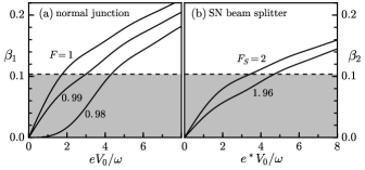
Figure 3: Violation of a generalized Bell inequality as a function of the harmonic drive amplitude: (a) normal junction with $G/G_{Q}=0.02$ and (b) SN beam splitter with $G_{S}/4G_{Q}=0.02$. Inequality is violated in the shaded regions in which $\beta_{1}$ and $\beta_{2}$ (solid lines) are smaller than $(\sqrt{2}-1)/4$ (dashed line).

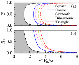
Figure 4: Generalized Bell test for a single-channel contact: (a) normal junction and (b) SN beam splitter. Results are shown for different shapes of the drive with the amplitude $V_{0}$. The biharmonic voltage $V(t)=V_{0}[0.8\cos(\omega t)+0.1\cos(3\omega t)]$ is an approximation of the triangle-wave drive. The regions to the left of the displayed lines are where the generalized Bell inequality is violated.

The inequality Eq. (2) can also be violated beyond the low-conductance limit in a quantum point contact with only a few discrete transport channels $T_{n}$. In the case of a single-channel contact, the parameters $X_{i}$ in Eq. (2) read $X_{1}=TR(\sum_{k}p_{k}+F_{p}-1)$ for the normal junction and $X_{2}=(R_{A}/4)(\sum_{k}p_{k}+F_{p}-1)$ for the SN beam splitter. The generalized Bell test is shown in Fig. 4 as a function of the contact transparency, amplitude of the drive, and for different shapes of the drive voltage. In the normal junction, violation of Eq. (2) occurs mostly in contacts that are either open or closed. This is because the probability of a successful Bell test is proportional to $TR$ which corresponds to one particle from a pair being transmitted to Bob while the other one is reflected to Alice, or vice versa. If this probability is sufficiently low, the signal from one entangled pair is not obscured by other pairs and Eq. (2) is violated. Similarly, the Bell test in the SN beam splitter geometry is realized by the injection of entangled pairs of electrons or holes with probability $R_{A}$ towards Alice and Bob. A violation of Eq. (2) occurs mainly in SN contacts with small $R_{A}$, in which the signal from one entangled pair is singled out from the rest. As regards the shape of the drive, we note that the square-wave drive creates more electron-hole pairs per cycle than the harmonic, sawtooth, or triangle-wave drive of the same amplitude, which decreases the chances of entangled pair detection. In the single-channel contact with low ac voltage, Eq. (2) is violated for any contact transparency. This is expected because in this case there is at most one electron-hole pair created and detected per voltage cycle, see Fig. 2.

Finally, we would like to come back to the effect of a finite temperature $T_{e}$, since one expects that the entanglement detection will become more difficult if not impossible for increased temperatures. To this end, we have evaluated the correlators in Eq. (4) for a normal junction in the tunnel limit $\{T_{n}\}\ll 1$ and at arbitrary temperature sup . The inequality is cast in the form $(\sqrt{2}-1)/4\leq\beta_{T_{e}}$, where we defined a new, temperature-dependent factor $\beta_{T_{e}}^{2}=\frac{G}{2G_{Q}}\sum_{l}|\textnormal{{g}}_{l}|^{2}l\coth(\frac{l\omega}{2T_{e}})$ with $\textnormal{{g}}_{l}$ being the Fourier coefficients of the phase $e^{i\int_{0}^{t}eV(t^{\prime})dt^{\prime}}$. The results are shown in Fig. (5). In the panel (a) an overview of the regions of entanglement detection in the conductance-voltage drive plot is given for different temperatures. An increasing temperature makes it more difficult to violate the inequality. For a given conductance, this leads to a prediction of a critical temperature of entanglement Beenakker (2006), above which detection of entanglement is not possible. However, the numerical values still allow a violation for an experimentally accessible temperature range $T_{e}\lesssim\omega$.

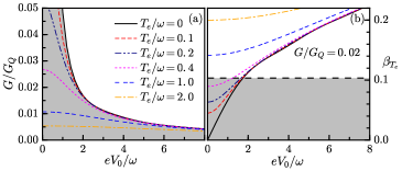
Figure 5: Effect of a finite temperature on the violation of the generalized Bell inequality for a harmonic drive. (a) The voltage ranges of violation (to the left of the respective curves) are reduced by a finite temperature. (b) For a fixed conductance a violation is only possible below a certain critical temperature for entanglement generation.

In conclusion, we have developed a continuous-variable entanglement test which does not require charge quantization, single-particle detection, or unidirectional particle flow and is therefore suitable for entanglement detection in ac driven systems. This is in stark contrast to previous proposals, which were unrealistic due to temperature restrictions in experiment. In contrast, an ac drive mixes electron states of different energies and leads to a complex entangled state consisting of electron- and holelike quasiparticle pairs Vanević et al. (2016). We have shown that the entanglement between electrons and holes in this situation can be probed using a four-terminal normal-metal junction, while the SN beam splitter can be used to reveal the entanglement of Cooper pairs emitted or absorbed by the superconductor. The success of entanglement detection relies on the ability to differentiate between the overall current fluctuations and the specific current correlations coming from the entangled pairs. This can be achieved in quantum contacts with low conductance or a small number of transport channels and with an ac drive which creates few electron-hole pairs per cycle. We have investigated the feasibility of the entanglement test for a cosine, square, sawtooth, and triangle drive. The ac drive affects the entanglement test through the total number of electron-hole pairs and the distribution of the pair creation probabilities. Finally, we have shown that our proposed entanglement test is robust against a finite temperature in the experimentally accessible regime. A promising platform for the observation might be driven cold atomic quantum point contacts in which single-particle or -spin detection seems feasible.Lebrat et al. ; Krinner et al. (2017) In the future, it might be interesting to connect our findings to efforts to quantify many-body entanglement in correlated electron systems, which are so far based mainly on experimentally inaccessible quantities.

We gratefully acknowledge the support from DFG through SFB 767 and the Serbian Ministry of Science Project No. 171027.

I Supplemental material for ”Continuous-variable entanglement test in a driven quantum contact”

Here we present the derivation of Eq. (3) of the main text for the cumulant generating functions ${\cal S}_{i}$ of the normal junction and the superconductor – normal-metal beam splitter and discuss the finite-temperature effect on the normal junction. In the end, we also discuss the Bell test for a single-channel normal-metal beam splitter.

II Normal-metal junction

The junction is schematically depicted in Fig. 1(a) of the main text. There are 4 leads: 2 left leads for Alice and 2 right leads for Bob. We assume the leads are perfectly spin filtered in directions $\pm\bm{a}$ and $\pm\bm{b}$ where $|\bm{a}|=|\bm{b}|=1$. We count charges that enter each of the leads and assign the counting fields $\chi_{j}^{\sigma}$ ($j=A,B$; $\sigma=\uparrow,\downarrow$) to them. The leads are characterized by the Keldysh-Green’s functions

$${\check{G}}_{L}(\chi_{A}^{\sigma}) =e^{-i\chi_{A}^{\sigma}\check{\tau}_{1}/2}\,{\check{G}}_{L}(0)\,e^{i\chi_{A}^{\sigma}\check{\tau}_{1}/2},$$ (7)

$${\check{G}}_{R}(\chi_{B}^{\sigma}) =e^{-i\chi_{B}^{\sigma}\check{\tau}_{1}/2}\,{\check{G}}_{R}(0)\,e^{i\chi_{B}^{\sigma}\check{\tau}_{1}/2},$$ (8)

where

$${\check{G}}_{l}(0)=\begin{pmatrix}1&2h_{l}\\ 0&-1\end{pmatrix}.$$ (9)

Here, $\check{\tau}_{1}$ is the first Pauli matrix in Keldysh space and $f_{l}=(1-h_{l})/2$ ($l=L,R$) are the generalized nonequilibrium distribution functions which depend on two time or energy indices. For an ac driven junction, we can use $2\times 2$ representation of $h_{L}$ and $h_{R}$ in energy space Vanević et al. (2007); *vanevic_elementary_2008

$$h_{L}=\begin{pmatrix}0&e^{-i\alpha_{k}}\\ e^{i\alpha_{k}}&0\end{pmatrix},\quad h_{R}=\begin{pmatrix}0&1\\ 1&0\end{pmatrix},$$ (10)

where $p_{k}=\sin^{2}(\alpha_{k}/2)$ ($k=1,2,\ldots$) are the probabilities of electron-hole pair creations. Note that the Green’s functions ${\check{G}}_{l}$ are scalars in the spin space.

For simplicity, we assume that the conductances of the spin filters are much larger than the one of the central junction $g=(e^{2}/\pi)\sum_{n}T_{n}$. In this case, the electron which arrives at Alice or Bob will enter the spin-polarized leads without backscattering. Since $A$ is strongly coupled to the spin-filtering leads and only weakly coupled to $B$, we can obtain the Green’s function ${\check{G}}_{A}$ of the node $A$ with the node $B$ disconnected. In addition, we assume that the spin filters have the same conductance and that an electron can enter any of the spin-filtering leads with equal probability. The Green’s function ${\check{G}}_{A}$ is obtained from the matrix current conservation $[(1+\bm{a}\cdot\hat{\bm{\sigma}}){\check{G}}_{L}(\chi_{A}^{\uparrow})+(1-\bm{a}\cdot\hat{\bm{\sigma}}){\check{G}}_{L}(\chi_{A}^{\downarrow}),{\check{G}}_{A}]=0$ and the normalization condition ${\check{G}}_{A}^{2}=\check{1}$ Lorenzo and Nazarov (2005). Here, $\hat{\bm{\sigma}}$ is the vector of Pauli matrices in spin space. We obtain

$${\check{G}}_{A}(\chi_{A}^{\uparrow},\chi_{A}^{\downarrow})=\frac{1+\bm{a}\cdot\hat{\bm{\sigma}}}{2}{\check{G}}_{L}(\chi_{A}^{\uparrow})+\frac{1-\bm{a}\cdot\hat{\bm{\sigma}}}{2}{\check{G}}_{L}(\chi_{A}^{\downarrow}),$$ (11)

and similarly for the node $B$,

$${\check{G}}_{B}(\chi_{B}^{\uparrow},\chi_{B}^{\downarrow})=\frac{1+\bm{b}\cdot\hat{\bm{\sigma}}}{2}{\check{G}}_{R}(\chi_{B}^{\uparrow})+\frac{1-\bm{b}\cdot\hat{\bm{\sigma}}}{2}{\check{G}}_{R}(\chi_{B}^{\downarrow}).$$ (12)

Cumulant generating function for the normal-metal junction is given by

$${\cal S}_{1}(\chi)=\frac{1}{2}\sum_{n}{\rm Tr}\ln\left(\check{1}+\frac{T_{n}}{4}(\{{\check{G}}_{A},{\check{G}}_{B}\}-2)\right),$$ (13)

where the trace is taken over Keldysh, spin, and energy indices. Since Alice and Bob are measuring the differences between the spin-up and spin-down charges, $\hat{A}\equiv\hat{N}_{A}^{\uparrow}-\hat{N}_{A}^{\downarrow}=\int dt(\hat{I}_{A}^{\uparrow}-\hat{I}_{A}^{\downarrow})/e$ and $\hat{B}\equiv\hat{N}_{B}^{\uparrow}-\hat{N}_{B}^{\downarrow}=\int dt(\hat{I}_{B}^{\uparrow}-\hat{I}_{B}^{\downarrow})/e$, we can set $\chi_{A}^{\uparrow}=\chi_{A}$, $\chi_{A}^{\downarrow}=-\chi_{A}$, $\chi_{B}^{\uparrow}=\chi_{B}$, and $\chi_{B}^{\downarrow}=-\chi_{B}$, where $\chi_{A}$ and $\chi_{B}$ are the counting fields related to the statistics of $\hat{A}$ and $\hat{B}$.

To compute ${\cal S}_{1}$, we proceed as follows. We note that ${\check{G}}_{A}$ and ${\check{G}}_{B}$ are $8\times 8$ matrices in Keldysh $\times$ spin $\times$ energy space. Cumulant generating function ${\cal S}_{1}$ can be written as a sum ${\cal S}_{1}={\cal S}_{1}^{+}+{\cal S}_{1}^{-}$, where

$${\cal S}_{1}^{\pm}(\chi_{A},\chi_{B})=\frac{1}{2}\sum_{n}{\rm Tr}\ln\left(\check{1}\pm\frac{\sqrt{T_{n}}}{2}({\check{G}}_{A}-{\check{G}}_{B})\right).$$ (14)

It turns out that $\check{1}\pm(\sqrt{T_{n}}/2)({\check{G}}_{A}-{\check{G}}_{B})$ have the same eigenvalues, hence ${\cal S}_{1}^{+}={\cal S}_{1}^{-}$. Moreover, the eigenvalues are pairwise equal to each other, $\lambda_{1}=\lambda_{2}$, $\lambda_{3}=\lambda_{4}$, $\lambda_{5}=\lambda_{6}$, and $\lambda_{7}=\lambda_{8}$. We obtain that the product $\lambda_{1}\lambda_{3}\lambda_{5}\lambda_{7}=1+2p_{k}T_{n}R_{n}[\cos(\chi_{A})\cos(\chi_{B})-1+\bm{a}\cdot\bm{b}\sin(\chi_{A})\sin(\chi_{B})]$. Therefore, the cumulant generating function reads

$${\cal S}_{1}(\chi_{A},\chi_{B})=\frac{\tau\omega}{\pi}\sum_{n,k}\ln\Big{(}1+2p_{k}T_{n}R_{n}\\ \times[\cos(\chi_{A})\cos(\chi_{B})-1+\bm{a}\cdot\bm{b}\sin(\chi_{A})\sin(\chi_{B})]\Big{)}.$$ (15)

This expression reduces to Eq. (3) of the main text.

III Superconductor – normal-metal beam splitter

The junction consists of a superconductor ($S$) coupled to the normal-metal lead ($N$) through the central junction characterized by transmission eigenvalues $\{T_{n}\}$. The normal lead is split into 4 outgoing terminals with spin filters along directions $\pm\bm{a}$ (Alice) and $\pm\bm{b}$ (Bob), see Fig. 1(b). As before, we assume strong coupling of the spin filters to the node $N$ and neglect the backscattering. We also assume that the spin-filtering leads have the same conductance. The cumulant generating function is given by

$${\cal S}_{2}(\chi)=\frac{1}{4}\sum_{n}{\rm Tr}\ln\left(1+\frac{T_{n}}{4}(\{\bm{G}_{S}(0),\bm{G}_{N}(\chi)\}-2)\right),$$ (16)

where the trace is taken in electron-hole (Nambu), Keldysh, spin, and energy indices.

At energies and temperatures much smaller than the gap, the Green’s function $\bm{G}_{S}$ of the superconductor is given by

$$\bm{G}_{S}(0)=\bar{\tau}_{2}\otimes\check{1}=\begin{pmatrix}0&-i\check{1}\\ i\check{1}&0\end{pmatrix},$$ (17)

where the block-matrix structure is in electron-hole space. The Green’s function $\bm{G}_{N}(\chi)$ of the node $N$ in the normal terminal is given by the matrix current conservation

$$\left[\begin{pmatrix}{\check{G}}_{Ae}+{\check{G}}_{Be}&0\\ 0&-({\check{G}}_{Ah}+{\check{G}}_{Bh})\end{pmatrix},\bm{G}_{N}\right]=0$$ (18)

and the normalization condition $\bm{G}_{N}^{2}=1$. Here, the Green’s functions for electrons and holes are given by

$${\check{G}}_{Ae} =\frac{1+\bm{a}\cdot\hat{\bm{\sigma}}}{2}{\check{G}}_{e}(\chi_{A}^{\uparrow})+\frac{1-\bm{a}\cdot\hat{\bm{\sigma}}}{2}{\check{G}}_{e}(\chi_{A}^{\downarrow}),$$ (19)

$${\check{G}}_{Be} =\frac{1+\bm{b}\cdot\hat{\bm{\sigma}}}{2}{\check{G}}_{e}(\chi_{B}^{\uparrow})+\frac{1-\bm{b}\cdot\hat{\bm{\sigma}}}{2}{\check{G}}_{e}(\chi_{B}^{\downarrow}),$$ (20)

and

$${\check{G}}_{Ah} =\frac{1-\bm{a}\cdot\hat{\bm{\sigma}}}{2}{\check{G}}_{h}(-\chi_{A}^{\uparrow})+\frac{1+\bm{a}\cdot\hat{\bm{\sigma}}}{2}{\check{G}}_{h}(-\chi_{A}^{\downarrow}),$$ (21)

$${\check{G}}_{Bh} =\frac{1-\bm{b}\cdot\hat{\bm{\sigma}}}{2}{\check{G}}_{h}(-\chi_{B}^{\uparrow})+\frac{1+\bm{b}\cdot\hat{\bm{\sigma}}}{2}{\check{G}}_{h}(-\chi_{B}^{\downarrow}).$$ (22)

We note that the counting fields and spin-polarization vectors for holes are the opposite from the ones for electrons. The counting fields are incorporated via the gauge transform ${\check{G}}_{e,h}(\chi)=e^{-i\chi\bar{\tau}_{3}\otimes\check{\tau}_{1}/2}\,{\check{G}}_{e,h}(0)\,e^{i\chi\bar{\tau}_{3}\otimes\check{\tau}_{1}/2}$, with

$${\check{G}}_{e}(0)=\begin{pmatrix}1&2UhU^{\dagger}\\ 0&-1\end{pmatrix},\quad{\check{G}}_{h}(0)=\begin{pmatrix}1&2U^{\dagger}hU\\ 0&-1\end{pmatrix}.$$ (23)

Here, $U(t^{\prime},t^{\prime\prime})=\exp[-i\int_{0}^{t^{\prime}}eV(t)dt]\delta(t^{\prime}-t^{\prime\prime})$ is unitary operator which takes into account the time-dependent drive Vanević et al. (2007); *vanevic_elementary_2008.

From Eq. (18) we obtain

$$\bm{G}_{N}=\begin{pmatrix}{\check{G}}_{Ne}&0\\ 0&-{\check{G}}_{Nh}\end{pmatrix},\quad{\check{G}}_{Ne,h}=\frac{{\check{G}}_{Ae,h}+{\check{G}}_{Be,h}}{2}.$$ (24)

Substituting this result in Eq. (16) and after taking the trace over electron-hole indices we find

$${\cal S}_{2}=\frac{1}{2}\sum_{n}{\rm Tr}\ln\left(\check{1}+\frac{\sqrt{R^{A}_{n}}}{2}\Big{(}{\check{G}}_{Ne}(2V(t))-{\check{G}}_{Nh}(0)\Big{)}\right).$$ (25)

Here, the remaining trace is taken over Keldysh, spin, and energy indices and $R^{A}_{n}=T_{n}^{2}/(2-T_{n})^{2}$ are the coefficients of Andreev reflections. In Eq. (25) we have also performed a gauge transform under the trace and ascribed the effect of the voltage drive to the electron part of the Green’s function, which leads to an effective voltage (or charge) doubling Belzig and Vanević (2016). After diagonalization of the operator in Eq. (25), we obtain

$${\cal S}_{2}(\chi_{A},\chi_{B})=\frac{\tau\omega}{\pi}\sum_{n,k}\ln\bigg{(}1+\frac{p_{k}R^{A}_{n}}{4}\\ \times\sum_{\alpha,\beta=\pm 1}\frac{1+\alpha\beta\bm{a}\cdot\bm{b}}{2}(e^{i\alpha\chi_{A}-i\beta\chi_{B}}-1)\bigg{)}.$$ (26)

This expression coincides with Eq. (3) of the main text.

IV Finite temperature effect on normal-metal junction

At finite temperature, $h_{L}$ and $h_{R}$ cannot be written as $2\times 2$ matrices because the involution property does not hold: $h^{2}_{L}\neq h^{2}_{R}\neq 1$. In energy representation, they are written as Vanević et al. (2008)

$$h_{L}(\epsilon^{\prime},\epsilon^{\prime\prime})=\sum_{l,m}\textnormal{{g}}_{l}\textnormal{{g}}^{*}_{l+m}h(\epsilon^{\prime}-l\omega-e\bar{V})2\pi\delta(\epsilon^{\prime\prime}-\epsilon^{\prime}-m\omega)$$ (27)

$$h_{R}(\epsilon^{\prime},\epsilon^{\prime\prime})=h(\epsilon^{\prime})2\pi\delta(\epsilon^{\prime}-\epsilon^{\prime\prime})$$ (28)

where

$$h(\epsilon)=\tanh\left({\frac{\epsilon}{2T_{e}}}\right)$$ (29)

and $\textnormal{{g}}_{l}$ is the $l$th coefficient of the Fourier series of the ac phase $e^{i\phi(t)}=\sum_{l}\textnormal{{g}}_{l}e^{-il\omega t}$ and $\phi(t)=\int^{t}_{0}e\Delta V(t^{\prime})dt^{\prime}$. In tunnel limit, the cumulant generating function Eq. (13) becomes

$${\cal S}_{1}(\chi)\approx\frac{1}{4}\frac{G}{G_{Q}}Tr_{\epsilon}({\check{G}}_{A}{\check{G}}_{B})$$ (30)

where the trace $Tr_{\epsilon}$ is taken in energy indices. After substituting Eqs. (27)-(29) into ${\cal S}_{1}$ and integration over energy, we have

$${\cal S}_{1}(\chi)= \frac{G}{G_{Q}}\sum_{l}|\textnormal{{g}}_{l}|^{2}l\coth(\frac{l\omega}{2T_{e}})$$

$$\times[\cos(\chi_{A})\cos(\chi_{B})+\bm{a}\cdot\bm{b}\sin(\chi_{A})\sin(\chi_{B})-1]$$ (31)

Here we have assumed zero dc bias. Eq. (IV) could be equivalently written as

$${\cal S}_{1}(\chi)= \frac{G}{2G_{Q}}\sum_{l}|\textnormal{{g}}_{l}|^{2}l\coth(\frac{l\omega}{2T_{e}})$$

$$\times\sum_{\alpha,\beta=\pm 1}\frac{1+\alpha\beta\bm{a}\cdot\bm{b}}{2}\left(e^{i\alpha\chi_{A}-i\beta\chi_{B}}-1\right)$$ (32)

Taking derivatives of Eq. (IV) with respect to the counting fields, we have the relations between the cumulants

$$\llangle A^{2n}\rrangle= \llangle B^{2n}\rrangle=\llangle A^{2n}B^{2n}\rrangle=\frac{G}{G_{Q}}\sum_{l}|\textnormal{{g}}_{l}|^{2}l\coth(\frac{l\omega}{2T_{e}})$$ (33)

$$\llangle AB\rrangle= \llangle A^{3}B\rrangle=\llangle AB^{3}\rrangle=-\bm{a}\cdot\bm{b}\llangle A^{2n}\rrangle$$ (34)

Choosing the angles between spin-polarization directions $\theta_{\bm{a}\bm{b}}=\theta_{\bm{a}^{\prime}\bm{b}}=\theta_{\bm{a}\bm{b}^{\prime}}=\pi/4$ and $\theta_{\bm{a}^{\prime}\bm{b}^{\prime}}=3\pi/4$, the generalized Bell inequality (Eq. (4) of the main text) reduces to

$$\frac{2-\sqrt{2}}{4}\leq\frac{\langle A^{2}\rangle}{\sqrt{\langle A^{4}\rangle}}$$ (35)

Let $X_{T_{e}}=\frac{G}{2G_{Q}}\sum_{l}|\textnormal{{g}}_{l}|^{2}l\coth(\frac{l\omega}{2T_{e}})$, Eq. (35) can be rewritten as

$$\frac{\sqrt{2}-1}{4}\leq\sqrt{\frac{X_{T_{e}}}{1+6X_{T_{e}}}}$$ (36)

which takes the same form of Eq. (2) of the main text. In tunnel limit, $G/G_{Q}\ll 1$, thus Eq. (36) can be approximately written as $(\sqrt{2}-1)/4\leq\beta_{T_{e}}$ where $\beta_{T_{e}}^{2}=X_{T_{e}}$.

V Bell test for a single-channel normal-metal beam splitter

In the following we analyze a normal-metal beam splitter analogous to the superconducting one shown in Fig. 1(b) of the main text. It has been found in Chtchelkatchev et al. (2002) that the normal beam splitter is not suitable for detection of entangled electron spin singlets injected by a dc voltage Lorenzo and Nazarov (2005). We show that this setup is inefficient in a driven case as well. For the cumulant generating function we find ${\cal S}_{N}(\chi_{A},\chi_{B})=M\sum_{n,k}\ln[1+(p_{k}T_{n}R_{n}/2)(e^{i\chi_{A}}+e^{-i\chi_{A}}+e^{i\chi_{B}}+e^{-i\chi_{B}}-4)+(p_{k}T_{n}^{2}/8)\sum_{\alpha,\beta=\pm 1}(1+\alpha\beta\bm{a}\cdot\bm{b})(e^{i\alpha\chi_{A}-i\beta\chi_{B}}-1)]$. The charge transfer statistics consists of two parts. The spin-dependent part is proportional to $p_{k}T_{n}^{2}$ and is related to the Bell-type events in which both electron and hole from a pair are transmitted to Alice and Bob. The spin-independent part is proportional to $p_{k}T_{n}R_{n}$ and describes events in which only one particle is transmitted to Alice or Bob while the other one is reflected back at the contact. These events carry no information on the particle spin correlations and lead to current fluctuations which obscure entanglement detection. Therefore, a violation of a generalized Bell inequality can be achieved only in a normal beam splitter of large transparency. For a single-channel junction with transmission coefficient $T$, Eq. (4) of the main text reduces to $1-1/\sqrt{2}\leq 2R/(1+3X_{p}/2)+2\sqrt{(2R+X_{p}/2)/(1+3X_{p}/2)}$, where $X_{p}=\sum_{k}p_{k}+F_{p}-1$. This inequality is violated for $T>0.99$ when Bell-type events dominate over particle reflections at the contact, see Fig. 6.

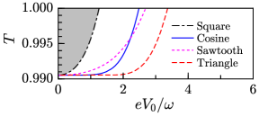
Figure 6: Generalized Bell test for a single-channel normal-metal beam splitter. Results are shown for different shapes of the drive with the amplitude $V_{0}$. The generalized Bell inequality is violated in the regions above the displayed lines where contact transparencies are very close to $T=1$.

VI Bell test for normal-metal junction with finite-polarized spin filters

In this section we consider the normal junction where the spin filters are not fully-polarized, namely $\bm{a}=\mathcal{P}\bm{m_{a}}$ and $\bm{b}=\mathcal{P}\bm{m_{b}}$ where spin polarization $0\leq\mathcal{P}\leq 1$ and $|\bm{m_{a}}|=|\bm{m_{b}}|=1$. The cumulant generating function is given by Eqs. (11) - (13) where $\chi_{A}^{\uparrow}=-\chi_{A}^{\downarrow}=\chi_{A}$ and $\chi_{B}^{\uparrow}=-\chi_{B}^{\downarrow}=\chi_{B}$. For the cumulant generating function we find

$${\cal S}_{1}(\chi)=\sum_{n,k}\ln\Big{[}1+2T_{n}(1-T_{n})p_{k}\\ \times[\cos(\chi_{A})\cos(\chi_{B})-1+\bm{m_{a}}\cdot\bm{m_{b}}\mathcal{P}^{2}\sin(\chi_{A})\sin(\chi_{B})]\\ +\frac{T_{n}^{2}}{2}p_{k}(1-\mathcal{P}^{2})[\cos(2\chi_{A})+\cos(2\chi_{B})-2]+\frac{T_{n}^{2}}{4}p_{k}^{2}(1-\mathcal{P}^{2})^{2}\\ \times[1-\cos(2\chi_{A})-\cos(2\chi_{B})+\cos(2\chi_{A})\cos(2\chi_{B})]\Big{]}.$$ (37)

Note that for $\mathcal{P}\neq 1$ there are no simple relations between the cumulants. In the low conductance limit and by choosing the angles between spin-polarization directions $\theta_{\bm{a}\bm{b}}=\theta_{\bm{a}^{\prime}\bm{b}}=\theta_{\bm{a}\bm{b}^{\prime}}=\pi/4$ and $\theta_{\bm{a}^{\prime}\bm{b}^{\prime}}=3\pi/4$, the generalized Bell inequality reads

$$\frac{\sqrt{2}\mathcal{P}^{2}-1}{4}\leq\beta_{\mathcal{P}}$$ (38)

where

$$\beta_{\mathcal{P}}^{2}= (2-\mathcal{P}^{4})\frac{G}{G_{Q}}\sum_{k}p_{k}-(3-2\mathcal{P}^{2})(1-F_{p})(1-F)$$

$$+2(1-\mathcal{P}^{2})(1-F).$$ (39)

In the fully-polarized spin case $\mathcal{P}=1$, the above inequality reduces to Eq. (5) of the main text. The violations of the above inequality for different Fano factors are plotted in Fig. 7.

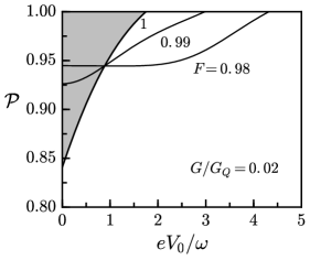
Figure 7: Generalized Bell test for a normal junction with finite polarization for harmonic drive. Fano factors $F=1,0.99,0.98$ are shown in the plot. The generalized Bell inequality is violated for spin polarizations and applied voltages that are above the lines.

References

- Einstein et al. (1935) A. Einstein, B. Podolsky, and N. Rosen, “Can quantum-mechanical description of physical reality be considered complete?” Phys. Rev. 47, 777 (1935).
- Bell (1964) J. S. Bell, “On the Einstein Podolsky Rosen paradox,” Phys. Phys. Fiz. 1, 195 (1964).
- Freedman and Clauser (1972) S. J. Freedman and J. F. Clauser, “Experimental Test of Local Hidden-Variable Theories,” Phys. Rev. Lett. 28, 938 (1972).
- Aspect et al. (1981) A. Aspect, P. Grangier, and G. Roger, “Experimental tests of realistic local theories via Bell’s theorem,” Phys. Rev. Lett. 47, 460 (1981).
- Aspect et al. (1982) A. Aspect, J. Dalibard, and G. Roger, “Experimental Test of Bell’s Inequalities Using Time-Varying Analyzers,” Phys. Rev. Lett. 49, 1804 (1982).
- Rarity and Tapster (1990) J. G. Rarity and P. R. Tapster, “Experimental Violation of Bell’s Inequality Based on Phase and Momentum,” Phys. Rev. Lett. 64, 2495 (1990).
- Rowe et al. (2001) M. A. Rowe, D. Kielpinski, V. Meyer, C. A. Sackett, W. M. Itano, C. Monroe, and D. J. Wineland, “Experimental violation of a Bell’s inequality with efficient detection,” Nature (London) 409, 791 (2001).
- Weihs et al. (1998) G. Weihs, T. Jennewein, C. Simon, H. Weinfurter, and A. Zeilinger, “Violation of Bell’s Inequality Under Strict Einstein Locality Conditions,” Phys. Rev. Lett. 81, 5039 (1998).
- Hensen et al. (2015) B. Hensen, H. Bernien, A. E. Dréau, A. Reiserer, N. Kalb, M. S. Blok, J. Ruitenberg, R. F. L. Vermeulen, R. N. Schouten, C. Abellán, W. Amaya, V. Pruneri, M. W. Mitchell, M. Markham, D. J. Twitchen, D. Elkouss, S. Wehner, T. H. Taminiau, and R. Hanson, “Loophole-free Bell inequality violation using electron spins separated by 1.3 kilometres,” Nature (London) 526, 682 (2015).
- Giustina et al. (2015) M. Giustina et al., “Significant-Loophole-Free Test of Bell’s Theorem with Entangled Photons,” Phys. Rev. Lett. 115, 250401 (2015).
- Shalm et al. (2015) L. K. Shalm et al., “Strong Loophole-Free Test of Local Realism,” Phys. Rev. Lett. 115, 250402 (2015).
- Collaboration (2018) The BIG Bell Test Collaboration, “Challenging local realism with human choices,” Nature (London) 557, 212 (2018).
- Steane (1998) A. Steane, “Quantum computing,” Rep. Prog. Phys. 61, 117 (1998).
- Bennett et al. (1993) C. H. Bennett, G. Brassard, C. Crépeau, R. Jozsa, A. Peres, and W. K. Wootters, “Teleporting an Unknown Quantum State via Dual Classical and Einstein-Podolsky-Rosen Channels,” Phys. Rev. Lett. 70, 1895 (1993).
- Boschi et al. (1998) D. Boschi, S. Branca, F. De Martini, L. Hardy, and S. Popescu, “Experimental Realization of Teleporting an Unknown Pure Quantum State via Dual Classical and Einstein-Podolsky-Rosen Channels,” Phys. Rev. Lett. 80, 1121 (1998).
- Gisin et al. (2002) N. Gisin, G. Ribordy, W. Tittel, and H. Zbinden, “Quantum cryptography,” Rev. Mod. Phys. 74, 145 (2002).
- Burkard et al. (2000) G. Burkard, D. Loss, and E. V. Sukhorukov, “Noise of entangled electrons: Bunching and antibunching,” Phys. Rev. B 61, R16303 (2000).
- Loss and Sukhorukov (2000) D. Loss and E. V. Sukhorukov, “Probing Entanglement and Nonlocality of Electrons in a Double-Dot via Transport and Noise,” Phys. Rev. Lett. 84, 1035 (2000).
- Recher et al. (2001) P. Recher, E. V. Sukhorukov, and D. Loss, “Andreev tunneling, Coulomb blockade, and resonant transport of nonlocal spin-entangled electrons,” Phys. Rev. B 63, 165314 (2001).
- Bena et al. (2002) C. Bena, S. Vishveshwara, L. Balents, and M. P. A. Fisher, “Quantum Entanglement in Carbon Nanotubes,” Phys. Rev. Lett. 89, 037901 (2002).
- Samuelsson et al. (2003) P. Samuelsson, E. V. Sukhorukov, and M. Büttiker, “Orbital Entanglement and Violation of Bell Inequalities in Mesoscopic Conductors,” Phys. Rev. Lett. 91, 157002 (2003).
- Samuelsson et al. (2004) P. Samuelsson, E. V. Sukhorukov, and M. Büttiker, “Two-particle Aharonov-Bohm Effect and Entanglement in the Electronic Hanbury Brown–Twiss Setup,” Phys. Rev. Lett. 92, 026805 (2004).
- Beenakker et al. (2003) C. W. J. Beenakker, C. Emary, M. Kindermann, and J. L. van Velsen, “Proposal for Production and Detection of Entangled Electron-Hole Pairs in a Degenerate Electron Gas,” Phys. Rev. Lett. 91, 147901 (2003).
- Beenakker et al. (2005) C. W. J. Beenakker, M. Titov, and B. Trauzettel, “Optimal Spin-Entangled Electron-Hole Pair Pump,” Phys. Rev. Lett. 94, 186804 (2005).
- Samuelsson et al. (2009) P. Samuelsson, I. Neder, and M. Büttiker, “Reduced and Projected Two-Particle Entanglement at Finite Temperatures,” Phys. Rev. Lett. 102, 106804 (2009).
- Klich and Levitov (2009) I. Klich and L. Levitov, “Quantum Noise as an Entanglement Meter,” Phys. Rev. Lett. 102, 100502 (2009).
- Hofstetter et al. (2009) L. Hofstetter, S. Csonka, J. Nygård, and C. Schönenberger, “Cooper pair splitter realized in a two-quantum-dot Y-junction,” Nature (London) 461, 960 (2009).
- Gabor et al. (2009) N. M. Gabor, Z. Zhong, K. Bosnick, J. Park, and P. L. McEuen, “Extremely efficient multiple electron-hole pair generation in carbon nanotube photodiodes,” Science 325, 1367 (2009).
- Herrmann et al. (2010) L. G. Herrmann, F. Portier, P. Roche, A. L. Yeyati, T. Kontos, and C. Strunk, “Carbon Nanotubes as Cooper-Pair Beam Splitters,” Phys. Rev. Lett. 104, 026801 (2010).
- Hofstetter et al. (2011) L. Hofstetter, S. Csonka, A. Baumgartner, G. Fülöp, S. d’Hollosy, J. Nygård, and C. Schönenberger, “Finite-Bias Cooper Pair Splitting,” Phys. Rev. Lett. 107, 136801 (2011).
- Simmons et al. (2011) S. Simmons, R. M. Brown, H. Riemann, N. V. Abrosimov, P. Becker, H.-J. Pohl, M. L. W. Thewalt, K. M. Itoh, and J. J. L. Morton, “Entanglement in a solid-state spin ensemble,” Nature (London) 470, 69 (2011).
- Das et al. (2012) A. Das, Y. Ronen, M. Heiblum, D. Mahalu, A. V. Kretinin, and H. Shtrikman, “High-efficiency Cooper pair splitting demonstrated by two-particle conductance resonance and positive noise cross-correlation,” Nat. Commun. 3, 1165 (2012).
- Schindele et al. (2012) J. Schindele, A. Baumgartner, and C. Schönenberger, “Near-Unity Cooper Pair Splitting Efficiency,” Phys. Rev. Lett. 109, 157002 (2012).
- Fülöp et al. (2015) G. Fülöp, F. Domínguez, S. d’Hollosy, A. Baumgartner, P. Makk, M. H. Madsen, V. A. Guzenko, J. Nygård, C. Schönenberger, A. Levy Yeyati, and S. Csonka, “Magnetic Field Tuning and Quantum Interference in a Cooper Pair Splitter,” Phys. Rev. Lett. 115, 227003 (2015).
- Gramich et al. (2017) J. Gramich, A. Baumgartner, and C. Schönenberger, “Andreev bound states probed in three-terminal quantum dots,” Phys. Rev. B 96, 195418 (2017).
- Clauser et al. (1969) J. F. Clauser, M. A. Horne, A. Shimony, and R. A. Holt, “Proposed Experiment to Test Local Hidden-Variable Theories,” Phys. Rev. Lett. 23, 880 (1969).
- Chtchelkatchev et al. (2002) N. M. Chtchelkatchev, G. Blatter, G. B. Lesovik, and T. Martin, “Bell inequalities and entanglement in solid-state devices,” Phys. Rev. B 66, 161320(R) (2002).
- Hannes and Titov (2008) W.-R. Hannes and M. Titov, “Finite-temperature Bell test for quasiparticle entanglement in the Fermi sea,” Phys. Rev. B 77, 115323 (2008).
- Bednorz and Belzig (2011) A. Bednorz and W. Belzig, “Proposal for a cumulant-based Bell test for mesoscopic junctions,” Phys. Rev. B 83, 125304 (2011).
- Lorenzo and Nazarov (2005) A. Di Lorenzo and Y. V. Nazarov, “Full Counting Statistics with Spin-Sensitive Detectors Reveals Spin Singlets,” Phys. Rev. Lett. 94, 210601 (2005).
- Vanević et al. (2007) M. Vanević, Y. V. Nazarov, and W. Belzig, “Elementary Events of Electron Transfer in a Voltage-Driven Quantum Point Contact,” Phys. Rev. Lett. 99, 076601 (2007).
- Vanević et al. (2008) M. Vanević, Y. V. Nazarov, and W. Belzig, “Elementary charge-transfer processes in mesoscopic conductors,” Phys. Rev. B 78, 245308 (2008).
- Belzig and Vanević (2016) W. Belzig and M. Vanević, “Elementary Andreev processes in a driven superconductor-normal metal contact,” Physica (Amsterdam) 82E, 222 (2016).
- Vanević and Belzig (2012) M. Vanević and W. Belzig, “Control of electron-hole pair generation by biharmonic voltage drive of a quantum point contact,” Phys. Rev. B 86, 241306(R) (2012).
- Vanević et al. (2016) M. Vanević, J. Gabelli, W. Belzig, and B. Reulet, “Electron and electron-hole quasiparticle states in a driven quantum contact,” Phys. Rev. B 93, 041416(R) (2016).
- Arakawa et al. (2015) T. Arakawa, J. Shiogai, M. Ciorga, M. Utz, D. Schuh, M. Kohda, J. Nitta, D. Bougeard, D. Weiss, T. Ono, and K. Kobayashi, “Shot Noise Induced by Nonequilibrium Spin Accumulation,” Phys. Rev. Lett. 114, 016601 (2015).
- (47) See Supplemental material.
- Beenakker (2006) C. W. J. Beenakker, “Electron-hole entanglement in the Fermi sea,” in Proceedings of the International School of Physics ”Enrico Fermi”, Vol. 162, edited by G. Casati, D. L. Shepelyansky, P. Zoller, and G. Benenti (IOS Press, Amsterdam, 2006) pp. 307–347.
- (49) M. Lebrat, S. Häusler, P. Fabritius, D. Husmann, L. Corman, and T. Esslinger, “Local spin manipulation of quantized atomic currents,” arXiv e-prints arXiv:1902.05516 [cond-mat.quant-gas] .
- Krinner et al. (2017) S. Krinner, T. Esslinger, and J. P. Brantut, “Two-terminal transport measurements with cold atoms,” J. Phys. Condens. Matter 29, 343003 (2017).