Generation of Magnetic Fields Near QCD Transition by Collapsing $Z(3)$ Domains

Abstract

In this work we investigate the possibility of generation of primordial magnetic field in the early universe near the QCD phase transition epoch via the collapse of $Z(3)$ domains. The $Z(3)$ domain walls arise in the deconfined phase of the QCD (above $T\sim 200$ MeV) and their collapse leads to a net quark concentration near the wall boundary due to non-trivial reflection of quarks. We look at the response of leptons to this quark excess and find that leptons do not cancel the electric charge concentration due to the quarks. The wall collapse and a net charge concentration can lead to the generation of vorticity and turbulence in the primordial plasma. We estimate the magnitude of the magnetic field generated and find that it can be quite large $\mathcal{O}(10^{15-18}\mathrm{G})$. The mechanism is independent of the order of the QCD phase transition.

1 INTRODUCTION

The origin of the observed magnetic fields in the Universe remains an unresolved problem of cosmology. Observations like Zeeman splitting of spectral lines, polarization and intensity measurement of of synchrotron radiation of electrons and Faraday rotation measurements indicate the presence of large scales magnetic fields in the universe. The strengths of these fields vary from $1-10~{}\mu$G for the length scales of the order of a few kpc to strengths of $\mathcal{O}(10^{-15}-10^{-18}\mathrm{G})$ for Mpc scales. The kpc scale field correlations can be explained by producing the seed magnetic fields using a Biermann battery mechanism in the proto galaxy, which are then amplified by a galactic dynamo. This process, however, fails for the large scale magnetic fields. An appealing alternative to the above scenario is to argue that the seed magnetic field has primordial origin which gets amplified as the proto galactic cloud undergoes collapse. This would naturally provide magnetic fields at all scales. For details, we refer to ref. Grasso:2000wj ; Widrow:2002ud ; Widrow:2011hs ; Subramanian:2015lua and the references cited therein.

The Universe has a rich thermal history and each of the stage can provide us the seed required to produce the observed magnetic field. In this work we focus on the epoch of the Quark-Hadron (Q-H) transition. This is expected to occur when the universe was roughly micro-seconds old. Till the turn of the century the Q-H transition was thought to be a first order transition. The bubble wall dynamics associated with the first order transition provided a rich spectrum of possibilities like quark nuggets as dark matter candidates Witten:1984rs , production of baryon inhomogeneities Fuller:1987ue and also the primordial magnetic fields Quashnock:1988vs ; Cheng:1994yr ; Sigl:1996dm . Unfortunately, none of the above scenarios hold in the light of results from lattice gauge theory showing that a first order quark-hadron transition is very unlikely. The transition, for the range of chemical potentials relevant for the early universe, is most likely a crossover. Thus there are no bubble walls and hence the entire spectrum of possibilities is relinquished. See ref. DeTar:2009ef ; Andersen:2014xxa ; DElia:2018fjp and references therein for details on the discussion of the order of the phase transition.

Our proposal for an alternate mechanism for the magnetic field generation is through the collapse of closed domain walls in the quark-gluon plasma (QGP) phase of QCD. An important point to note is that this mechanism does not depend on the order of the QCD phase transition as the domain walls are present in the QGP phase of the system and are not a result of the Q-H transition. Since these defects are in the deconfined phase of QCD and vanish in the confined phase, they are not constrained, unlike the GUT defects.

The possibility of extended topological objects in the QGP has been extensively discussed in the literature Bhattacharya:1992qb ; West:1996ej ; Boorstein:1994rc . These are domain wall defects that arise from the spontaneous breaking of $Z(3)$ symmetry in the high temperature phase (QGP phase) of QCD. We should mention that the existence of these $Z(3)$ walls becomes a non-trivial issue in the presence of quarks Smilga:1993vb ; Belyaev:1991np . However it has also been argued that the effect of quarks can be understood in terms of the explicit breaking of $Z(3)$ symmetry DeGrand:1983fk ; Dumitru:2003cf . This interpretation allows for very interesting possibilities for the QGP phase with rich phenomenology which can have very important implications for cosmology. This finds support in the recent lattice calculations of QCD with quarks Deka:2010bc and also in the effective model studies of QGP Mishra:2016ipq which suggest that there is a strong possibility of existence of these $Z(3)$ vacua at high temperature.

However the magnetic field produced during processess that happen before the QCD phase transition, like the electro-weak phase transition, might be present at the time of the Q-H transition (see reviews Grasso:2000wj ; Widrow:2002ud ; Widrow:2011hs ; Subramanian:2015lua and ref. Dolgov:2010gy ; Ayala:2017gqa for more recent works). In presence of magnetic field the QCD phase transition shows intriguing behaviour. The chiral condensate at $T=0$ grows monotonically with the magnetic field strength, an effect known as magnetic catalysis. At finite $T$ the situation gets a bit involved. Below critical temperature, the chiral condensate increases with magnetic field with values consistently smaller than those at $T=0$ for the same magnetic field strength. As $T$ approaches $T_{c}$, the chiral condensate reaches a peak value for a threshold value of magnetic filed and shows a reduction with further increase in the magnetic field. Above the critical temperature the chiral condensate decreases for all values of magnetic field. This phenomenon is termed as the inverse magnetic catalysis Andersen:2014xxa . The effective models of QCD phase transition do not reproduce this pattern quite well. Even though attempts have been made to explain the discrepancy between Lattice studies and the effective models by trying to separate the contributions of valance and sea quarks (see sec. IXA of ref. Andersen:2014xxa ), a final word still remains to be said. The magnetic field, through quark contribution, tends to break the $Z(3)$ symmetry explicitly Mizher:2010zb . Recent lattice results Endrodi:2015oba indicate that in the presence of an asymptotically large magnetic field, the transition is quite sharp (possibly a first order too) and is at a lower temperature than in the absence of a magnetic field. A similar effect is expected in the case of electro-weak phase transition in presence of magnetic field Ayala:2004dx ; Sanchez:2006tt . In such a situation it is quite possible that all the possibilities mentioned above are realised in the early universe near the Q-H transition. We refer to Andersen:2014xxa and references therein for a comprehensive discussion of QCD phase transition in a magnetic field.

Even when there is no magnetic field, $Z(3)$ defects can revive the first order transition scenarios of baryon inhomogeneities and quark nuggets formation Layek:2005zu ; Atreya:2014sca . We might add that these are the only relativistic field theory topological solitons which are accessible in laboratory experiments. Their detection will provide deep insights in the non-trivial physics of the QGP phase. It therefore looks reasonable to explore the possible consequences of these $Z(3)$ domains and associated walls.

As the $Z(3)$ domain wall collapses, it produces shocks in the plasma which will lead to turbulence being generated in the wake of the the wall. As the wall sweeps through the quark gluon plasma, an excess baryon concentration builds in the collapsing region. We use Poisson’s equation to estimate the electric charge, due to leptons, on the domain wall. We find that the lepton concentration doesn’t cancel the charge due to the baryon concentration. Assuming the domain wall collapse to be spherical, we calculate the magnetic field generated during the collapse. The magnetic field generated depends on the baryon density contrast across the domain wall and the size of the collapsing region. It can be as high as $10^{15-18}$ G for a baryon density contrast of the order of $10^{6}$ within a radius of roughly one meter. Since the collapse of the domain walls happen before the quark hadron phase transition, the magnetic field is generated in the quark gluon plasma epoch. Thus the mechanism is completely independent of the order of the phase transition.

The organization of the paper is as follows. In section 2 we briefly discuss the $Z(3)$ symmetry. This is the symmetry of the Polyakov loop which is the order parameter of the confinement transition. We estimate the profile of the domain wall and the transmission coefficients for different quarks. In section 3 we discuss the formation of $Z(3)$ structures in the early universe and how a charge density is accumulated within a collapsing $Z(3)$ domain In section 4, we first argue that these collapsing domains can generate the vorticity in the plasma and then make an estimate of the magnetic field generated. We conclude in section 5.

2 $Z(3)$ DEFECTS AND QUARK INTERACTIONS

2.1 $Z(3)$ domains in QGP

The order parameter of the confinement-deconfinement transition for a pure gauge $SU(N)$ system at temperature $T$, is the thermal expectation value of the Polyakov loop Polyakov:1978vu ; Gross:1980br ; McLerran:1981pb defined as

$$L(x)=\frac{1}{N}\mathrm{Tr}\left\{\mathbf{P}\biggl{[}\exp\left(ig\int_{0}^{\beta}A_{0}(\vec{x},\tau)d\tau\right)\biggr{]}\right\},$$ (1)

where $\beta=T^{-1}$ and and $g$ is the gauge coupling. The trace denotes the summing over color degrees of freedom and $\mathbf{P}$ denotes the path ordering in the Euclidean time $\tau$. The $SU(N)$ gauge fields satisfy the periodic boundary conditions in $\tau$, viz $A_{0}(\vec{x},0)=A_{0}(\vec{x},\beta)$.

The free energy of a test quark can then be studied by writing the partition function and noting that $\langle L(\vec{x})\rangle\propto e^{-\beta F}$. In the confined phase, $\langle L(\vec{x})\rangle=0$ implying that the free energy of a test quark is infinite (i.e. system is below $T_{c}$). In the deconfined phase, a test quark has finite free energy and hence $\langle L(\vec{x})\rangle\neq 0$. We will use $l(x)$ to denote $\langle L(\vec{x})\rangle$ from now on, for the sake of brevity. Under $Z(N)$ transformation (which is the center of $SU(N)$), $l(x)$ transforms as

$$l(x)\longrightarrow Z\times l(x),\qquad\text{where}~{}Z=e^{i\phi},$$ (2)

and $\phi=2\pi m/N$; $m=0,1\dotsc(N-1)$. This gives rise to the spontaneous breaking of $Z(N)$ symmetry with $N$ degenerate vacua in the deconfined phase, where $\langle L(\vec{x})\rangle\neq 0$. For QCD, $N=3$ and hence it has three degenerate $Z(3)$ vacua resulting from the spontaneous breaking of $Z(3)$ symmetry at $T>T_{c}$. This leads to the formation of interfaces between regions of different $Z(N)$ vacua. These vacua are characterized by, $l(\vec{x})=1,e^{2\pi i/3},e^{4\pi i/3}.$

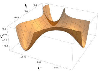
Figure 1: Effective potential of Polyakov loop for $T>T_{c}$. The plot is at $T=200$ MeV.

The effective potential for Polyakov loop which captures the basic features of $Z(3)$ structures is given by Pisarski:2000eq

$$V(l)=\biggl{(}-\frac{b_{2}}{2}|l|^{2}-\frac{b_{3}}{6}\Bigl{(}l^{3}+(l^{*})^{3}\Bigr{)}+\frac{1}{4}(|l|^{2})^{2}\biggr{)}b_{4}T^{4},$$ (3)

where $b_{2}=\left(1-1.11/x\right)\left(1+0.265/x\right)^{2}\left(1+0.300/x\right)^{3}-0.478$ (with $x=T/T_{c}$ with $T_{c}\sim 182$ MeV) ,$b_{3}=2.0$ and $b_{4}=0.6061\times 47.5/16$. The value of $T_{c}$ and the coefficients are fixed by fitting the energy and pressure to the lattice results Scavenius:2002ru . An overall factor of $(47.5)/16$ in $b_{4}$ is used to compensate for the change in the energy density by re-scaling the number of degrees of freedom for the three flavor case. In $T\longrightarrow\infty$ limit, $l\left(x\right)\longrightarrow y=b_{3}/2+\frac{1}{2}\times\sqrt{b_{3}^{2}+4b_{2}\left(T=\infty\right)}$. As $\lvert l(x)\rvert=\exp(-\beta\Delta F)$, $l(x)\longrightarrow 1$ in the limit $T\longrightarrow\infty$. We re-scale the quantities as

$$l\left(x\right)\rightarrow\frac{l\left(x\right)}{y},~{}~{}b_{2}\rightarrow\frac{b_{2}}{y^{2}},~{}~{}b_{3}\rightarrow\frac{b_{3}}{y},~{}~{}b_{4}\rightarrow b_{4}y^{4},$$

to get the desired asymptotic behavior of $l(x)$. Writing $l(x)=|l(x)|e^{i\theta}$, we see that $(l^{3}+(l^{*})^{3})=\cos(3\theta)$. This results in three degenerate $Z(3)$ vacua for $T>T_{c}$, as shown in fig 1.

2.2 Interaction of Quarks with the Domain Wall

We now discuss the interaction of the quarks with the domain wall. Fig 1 shows that $l(x)$ varies as we go from one vacua to other. As $\lvert l(x)\rvert=\exp(-\beta\Delta F)$ ($\Delta F$ being the change in the free energy of a quark); the change in the free energy of the quark as it traverses the domain wall is given by

$$\Delta F=-T\ln\left(\lvert l(x)\rvert\right)$$ (4)

A moving quark thus experiences an effective potential as it crosses the wall. To estimate $\Delta F$ we need the domain wall profile $l(x)$. For obtaining the $l(x)$ profile we use the energy minimization technique. We write, $l(x)=l_{1}(x)+\dot{\iota}l_{2}(x)$, then we express eq. (3) in terms of $l_{1}(x)$ and $l_{2}(x)$. We then start the linear interpolation with values of $l_{1},l_{2}$ between $\theta=0$ and $\theta=2\pi/3$ and minimize the total energy $\left((\nabla l)^{2}+V(l)\right)$ of the system. The numerical technique used to minimize energy is over relaxation technique. This technique requires that the field be fluctuated at a lattice site and then the change is observed in the energy density due to the fluctuation. With three such fluctuations a parabola is fitted. The minimum of the parabola provides the minimum energy configuration. The actual change in the field is taken as a fraction of this minimum value. We take the the fraction to be 0.05 times the field value obtained. The energy is then calculated with the new field values and the process is repeated till the energy stops changing effectively. The resultant $l(x)$ profile and the corresponding variation in the free energy are shown in fig 2.

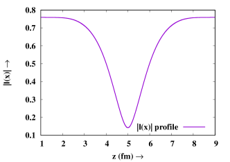
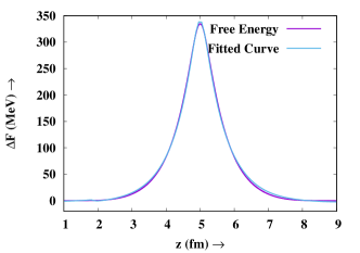
Figure 2: Top:- The $l(x)$ profile at $T=200$ MeV. Bottom:- The corresponding free energy change and the fitted curve (see text for details).

The free energy is fitted with a curve. The form of the function and the parameters are presented in Table 1. For more details on the process of obtaining $l(x)$ profile, we refer to Layek:2005fn .

Table 1: Table for the parameters used for fitting the free energy variation with the function $-200\ln\{\sqrt{[a\tanh(bx+c)+d]^{2}+[e\tanh(fx+g)+h)]^{2}}\}+p$

Parameter	Value
$\quad\quad a$	$1.0036$
$\quad\quad b$	$-0.739001$
$\quad\quad c$	$3.68957$
$\quad\quad d$	$0.00450475$
$\quad\quad e$	$-0.0898081$
$\quad\quad f$	$-14.4524$
$\quad\quad g$	$26.833$
$\quad\quad h$	$0.0916998$
$\quad\quad p$	$-0.381349$

This free energy change is like an effective potential ($V$) experienced by the quark as it traverses the domain wall. We approximate the $l(x)$ profile with a box of width $\sim 1$ fm and height $\sim 0.6$. This translates to an effective potential of width $a=1$ fm and height $\sim 305$ MeV. We use this potential to estimate the transmission coefficient. The analytic expression for the transmission coefficient for a free quark incident on a box potential is given by Mckellar:1987ru :

$$T =\frac{1}{\cos^{2}\left(Ka\right)+\frac{1}{4}\Big{\lvert}\frac{\Lambda}{\lambda}+\frac{\lambda}{\Lambda}\Big{\rvert}^{2}\lvert\sin(Ka)\rvert^{2}}~{};$$ (5a)

$$\mathrm{where}\quad\lambda =\frac{k}{E+m}~{};\quad\quad~{}~{}\Lambda=\frac{K}{(E-V)+m};$$ (5b)

$$\mathrm{with}\quad k =(E^{2}-m^{2})^{1/2}~{};\quad K=\left((E-V)^{2}-m^{2}\right)^{1/2}$$ (5c)

The transmission coefficients for u,d and s quarks are listed in Table 2. From Table 2, we conclude that the transmission coefficients of u/d quarks are higher than the transmission coefficient of the s-quarks.

The recent lattice results with quarks Bhattacharya:2014ara ; Steinbrecher:2018phh have reported slightly different values of $T_{c}$ than the value used above. It is then advisable to see how our results obtained above fare in the light of these results. We note that the $l(x)$ profile depends on the shape of the potential given in 3. Since the potential depends on the ratio $T/T_{c}$, it is this value which will be important, not the exact value of $T_{c}$, in determining the shape of the potential. For our case we are focusing on $T=200$ MeV, which translates to $T/T_{c}\sim 1.1$ for $T_{c}\sim 182$ MeV quoted in ref. Scavenius:2002ru . The shape of the profile will remain same for the corresponding $T$ which keeps the above value fixed. For $T_{c}\sim 155$ MeV, which is quoted in ref. Bhattacharya:2014ara ; Steinbrecher:2018phh , the corresponding $T\sim 170$ MeV, which is close to $T\sim 200$ MeV used by us. Thus we hope to capture the correct qualitative features of the $Z(3)$ symmetry in our analysis.

Also replacing a box function with a smooth profile would change the transmission coefficients. It was shown in Atreya:2011wn that for a step potential, the coefficients are larger than those for a smooth profile with the width $\sim 1$ fm. This essentially means that u and d quarks will essentially pass through and not get reflected while strange quarks will get reflected but with a lower probability, for a more realistic profile of the scattering potential. So qualitative features of the results will not change, as in that the concentration in the collapsing region would be solely because of strange quarks.

Table 2: Transmission for different quark flavors for incoming E $=500$ MeV.

$q$ flavor	$\quad\quad T$
$u/d$	$0.999329$
$s$	$0.855293$

3 Charge Inhomogeneity due to collapsing $Z(3)$ domains

In this section we discuss how a net charge is concentrated across the domain wall as it collapses. We start with a probable scenario of $Z(3)$ domain formation in early universe and their survivability till the QCD phase transition. We then estimate the density of quarks trapped inside the collapsing $Z(3)$ domains. Since quarks have electric charge too, their concentration leads to a electric charge concentration across the domain walls. We look at the response of the leptons to this baryon excess and find that leptons do not cancel this net electric charge concentration.

3.1 Formation of $Z(3)$ domains in early universe

The standard picture of defect formation in cosmology relies on the Kibble mechanism Kibble:1976sj . The defects are formed during the transition to the symmetry broken phase as the universe cools during its evolution. Since $Z(3)$ symmetry is broken in the high temperature phase, and is restored as the universe cools while expanding, the question then arises as to how these defects were formed. This question was first addressed in ref. Layek:2005zu .

The pre inflationary universe was in the deconfined state as $T>>T_{c}$. During inflation the universe cools exponentially and $Z(3)$ interfaces disappear as $T\rightarrow 0$. When temperature eventually becomes higher than $T_{c}$, during reheating, $Z(3)$ symmetry breaks spontaneously, and $Z(3)$ defects form via the Kibble mechanism. However quarks lead to an explicit breaking of $Z(3)$ symmetry. Two of the vacua, with $l(x)=z,~{}z^{2}$, become meta-stable leading to a pressure difference between the true vacuum and the meta-stable vacua Dixit:1991et . This leads to a preferential shrinking of the meta-stable vacua. The explicitly breaking of $Z(3)$ symmetry might get amplified in presence of magnetic field as discussed in section (1).

As the collapse of these closed regions can be very fast Gupta:2010pp ; Gupta:2011ag , they are unlikely to survive until late times, say until the QCD scale. However the dynamics of these $Z(3)$ walls might be friction dominated due to the non-trivial scattering of quarks from the domain wall. For large friction, they might survive till the late times. In certain low energy inflationary models with low reheating temperature Knox:1992iy ; Copeland:2001qw ; vanTent:2004rc , even a small friction in the domain walls collapse will allow the walls to survive until QCD transition. If these domains survive till late times (which cannot be below the QCD transition epoch), then the magnetic fields will be generated near the QCD transition epoch.

3.2 Number Density Evolution in the Collapsing Region

We now estimate the number density concentration within the collapsing region. We are interested in demonstrating a new method of generating magnetic fields from collapsing $Z(3)$ domain walls. To make an approximate estimate of the magnetic field generated in this method, we make some simplifying assumptions. The first one being that the collapse happens faster than the Hubble expansion rate, thus the universe is at a constant temperature. This means that the domain wall configuration can be taken as constant, since $l(x)$ depends on $T$ which is constant. This also means that one can neglect the expansion of the universe in the present context. Another assumption is that the particles thermalize instantaneously as they reflect from the wall. Finally we ignore the baryon diffusion in the plasma. This essentially translates to assumption that the baryons instantaneously homogenize after the collision with the wall.

Let there be $N$ domains with radius $R(t)$. Then the total volume within the domain is $V_{d}=N(4\pi/3)R(t)^{3}$. If $V$ is the Hubble volume, then $V-V_{d}\equiv V_{o}$ is the volume outside the region enclosed by domains. Let the number density of particles outside and inside the closed domains be $n_{o}$ and $n_{i}$. Then the rate of change of concentration is given by

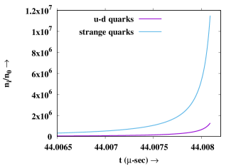
Figure 3: Build up of the quark number density inside the domain wall at $T=200$ MeV. The collapse velocity is chosen to be $0.5/\sqrt{3}$.

$$\dot{n_{i}}=\Bigl{(}-\frac{2}{3}v_{w}T_{w}n_{i}+\frac{v_{o}^{rel}n_{o}T_{-}-v_{i}^{rel}n_{i}T_{+}}{6}\Bigr{)}\frac{S}{V_{d}}-n_{i}\frac{\dot{V_{d}}}{V_{d}}\\$$ (6)

$$\dot{n_{0}}=\Bigl{(}\frac{2}{3}v_{w}T_{w}n_{i}-\frac{v_{o}^{rel}n_{o}T_{-}-v_{i}^{rel}n_{i}T_{+}}{6}\Bigr{)}\frac{S}{V_{d}}+n_{o}\frac{\dot{V_{d}}}{V_{o}},\\$$ (7)

where $v_{w}$ is the wall velocity, $S$ is the surface area of the enclosed region. The particle motion can be studied with components parallel to the wall $(v_{w})$ and perpendicular to the wall. $v_{o,i}^{rel}$ is the relative velocity of the particle (outside or inside), perpendicular w.r.t. the wall. Each particle has $6$ degrees of freedom with $4/6$ in the parallel direction and $1/6$ moving towards the wall, perpendicular to it. These are the ones that contribute to the change in the number density. The remaining $1/6$ are moving away from the wall and therefore do not contribute. The change in the domain volume $\dot{V}_{i}$ is estimated by looking at $R(t)$

$$R(t)=\frac{r_{H}}{N^{1/3}}-v_{w}(t-t_{0}),$$ (8)

where $r_{H}$ is the horizon size of the universe at $t=t_{0}\simeq 30\left(\frac{150}{T(MeV)}\right)^{2}$. $T_{w}$ are the reflection coefficient for the particles moving parallel to wall and $T_{-}(T_{+})$ are the transmission coefficients calculated for the quarks that are moving from outside (inside) of the wall towards the inside (outside).

We solve eq. (6), (7) and (8) simultaneously to get the increase in the charge concentration across the domain wall. We consider the wall velocity to be $0.5/\sqrt{3}$ and the number of domains within the horizon, $N=10$. The evolution of the number density normalized to the background number density is plotted in Fig. (3). One can clearly see the rise in the number density inside the collapsing region. The difference between the concentration of different quark species is also clearly visible. The entire concentration inside the domain can be attributed to the strange quarks that outnumber the other quark species by an order of magnitude. Since the $l(x)$ profile is color neutral, the effective potential as seen by quarks is also color neutral and thus the anti-quarks have the same concentration.

To estimate the density of quarks trapped in the collapsing domain, we look at the density profile left behind the collapsing domain. Let $\rho(r)$ be the particle density left behind the domain wall. Then total number of particles in a shell of thickness $dr$ at a distance $r$ from the center of domain wall is given by $dN=4\pi r^{2}\rho(r)dr$. This gives

$$\rho(r)=-\frac{\dot{N}}{4\pi r^{2}v_{w}}$$ (9)

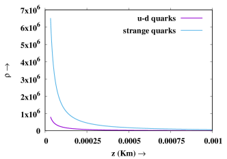
Figure 4: The density profile of the particles left behind by the domain wall at $T=200$ MeV. The collapse velocity is chosen to be $0.5/\sqrt{3}$.

The quark profile as the function of the radius of the collapsing region is shown in the Fig (4). We notice that almost the entire quark concentration can be solely owed to the strange quarks. The same profile will be obtained for the anti-quarks owing to the color neutral nature of the effective potential seen by quarks anti-quarks. However there is a small baryon asymmetry $(\sim 10^{-10})$ in the universe near QCD transition. Thus even though the density profile is same for the quarks and anti-quarks, there is a difference in their net numbers. We now make an order of magnitude estimates of quark over-densities. From Fig (4) we see that the density within a radius of $1$ m is roughly $10^{6}$ times the background density. At $T=200$ MeV, the corresponding length scale is $1$ fm, thus we take the background density to be $\sim 1$fm^-3 which is $10^{45}$ m^-3. Thus we get $\sim 10^{51}$ quarks within a radius of $1$ m which translates to an net excess baryon number of $10^{41}$.

The transmission coefficients from eq. (5a) appear directly in the eq. (6) and (7). Thus naively one can say that the rate of concentration of quarks will be slower for the realistic scenario as the transmission is larger there. This would mean that the charge pile up will take some more time to reach the values quoted in the fig. (3). This would translate to the size of domain wall thus effecting the density profile in fig (4). The numbers quoted there will be attained a bit later than the present case. However if the collapse is faster than what we consider it to be (which is likely as argued in sec 4.1), these high densities can be attained quite easily as $v^{rel}$ and $v_{w}$ in eq. (6) will compensate for the reduction in transmission coefficients. In either case the concentration quoted by us can be attained a bit sooner or later depending on how the realistic situation unfolds.

3.3 Dynamical Charge build up across the domain wall

As we discussed, quarks/anti-quarks undergo non-trivial reflection and transmission from $Z(3)$ domains. Thus there is a density contrast across the domain wall. We also argued that anti-quarks do not cancel this baryon excess due to tiny baryon asymmetry. Since quarks also carry electric charge, a density contrast across the interface also leads to a charge asymmetry due to the difference in charges of the u,d and s quarks. While the net baryon over-density is given by, $n_{B}=(n_{u}+n_{d}+n_{s})/3$, the net charge over-density is given by $\rho_{c}=e(2n_{u}-n_{d}-n_{s})/3$. Substituting, the over-densities of the respective quarks inside the $Z(3)$ domain walls, we find that $\rho_{c}\approx-10^{6}e$.

Due to this charge concentration, a potential is generated across the domain wall. We can use the Debye model to estimate the strength of the potential. We reiterate that since the quark hadron transition has not taken place as yet, the only charged particles in plasma are the quarks and leptons.

The strong interaction screening for QGP is effective at the length scale of $\sim 1$ fm, while it is different for the EM interactions. To estimate the EM Debye length we make the approximation that near the domain wall the electrons are moving in the background of quarks and muons which are much heavier than the electrons. In this approximation the situation is akin to that of an electron-ion plasma and one can use the following expression to estimate the Debye length

$$\lambda_{D}=\Biggl{[}\frac{1}{2\pi e^{2}\left(\frac{n_{e}}{T_{e}}+\sum_{i}\frac{q_{i}^{2}n_{i}}{T_{i}}\right)}\Biggr{]}^{1/2},$$ (10)

$n_{e}$ and $T_{e}$ are the temperatures of the electron and $q_{i},~{}n_{i},~{}T_{i}$ are the charge, number density and temperature of the ion species $i$. For us $T_{e}=T_{i}$ and $q_{i}=2/3,~{}-1/3,~{}-1/3$ and $-1$ for $u,~{}d,~{}s$ quarks and muon respectively. Since all particles are relativistic one can assume that $n_{e}\sim n_{i}$. This reduces the eq. (10) to

$$\lambda_{D}=\left(\frac{9T}{16\pi e^{2}n_{e}}\right)^{1/2},$$ (11)

Since the number density of fermions at temperature $T>>m$, the mass of electron, is $n_{i}\sim\frac{3\zeta(3)}{4\pi^{2}}T^{3}$ is (where $\zeta(3)$ is the Riemann zeta function). This translates to $\lambda_{D}\sim 10^{-9}$ m for $T\sim 200$ MeV.

The charge density of the quarks on the domain wall has been obtained in the previous section. For this charge density, one can solve the Poisson’s equation ($\frac{\partial^{2}\phi(x)}{\partial x^{2}}=-4\pi\times 10^{6}e$) numerically and obtain the potential $\phi(x)$. Here $x$ is the distance from the domain walls. This gives us the charge density profile for the quarks. Since the potential is now known, one can use the standard solution $n_{i}e^{(-\frac{e\phi}{T})}$to obtain the lepton profile in response to the charged potential. Here $n_{i}$ is the number density of leptons defined previously and $\phi$ is the numerical solution obtained previously. The numerical calculation is done using standard codes in R software. We note that the difference between the two profiles is not very large. However there exists a finite difference. To show that the lepton charges and the quark charges cannot cancel each other exactly, we plot the charge density scaled by a factor of $10^{6}$ for both the cases. Fig.5 shows the response of leptons to the charge build up of quarks near the domain wall. We see that the lepton charge density doesn’t cancel the quark charge density in the vicinity of the domain wall.

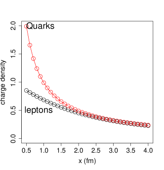
Figure 5: The quark density profile and the lepton density profile (scaled by $10^{6}$) near the domain wall.

4 Magnetic field generation

In this section we will take a look at the magnetic field generation in the QGP phase due to the collapse of the $Z(3)$ domain walls. We first argue that the collapse of the domain walls lead to turbulence in the plasma and then estimate the strength of the magnetic field due to the charge build up around the collapsing domain walls.

4.1 Turbulence Generation by Collapsing Domains

A closed surface collapses due to the surface tension $\sigma$, and the energy difference between the enclosed region and the outside, $\epsilon$. One can then write the Lagrangian for the domain wall as Adams:1989su ,

$$L=-4\pi\sigma R^{2}(1-\dot{R}^{2})^{1/2}+\frac{4\pi}{3}R^{3}\epsilon$$ (12)

The equation of motion for a perfectly spherical wall is then

$$\ddot{R}=\frac{\epsilon}{\sigma}\left(1-\dot{R}^{2}\right)^{3/2}-\frac{2}{R}\left(1-\dot{R}^{2}\right).$$ (13)

On integrating the above equation we get the velocity of the domain wall as a function of its radius.

$$\left(1-\dot{R}^{2}\right)^{1/2}=\frac{R^{2}}{\epsilon R^{3}/3\sigma+\mathrm{constant}},$$ (14)

As the domain wall collapses $R\rightarrow 0$, and $|\dot{R}|\rightarrow 1$. As a result when a spherical domain collapses, it will produce shocks in the cosmic plasma. Turbulence is generated in the wake of the shocks. The shocks in the charge concentration left behind the collapsing region will then generate the magnetic field.

If the dynamics of domain walls is friction dominated, like the scenario above where the collapse will be slow and for which we have estimated the quark densities, the shocks will not be produced in the plasma. Even then there would be turbulence produced near the surface of the domain wall. The momentum equation for the velocity field is given by,

$$\frac{\partial\vec{u}}{\partial t}+\vec{u}.\nabla{u}=-\frac{\nabla p}{\rho}+\vec{F_{visc}}.$$ (15)

Here $\rho$ is the density of the fluid, $\nabla p$ is the change in pressure and $\vec{u}$ is the velocity field of the fluid particles. For simplification, let us assume that the viscous forces $\vec{F_{visc}}$ are negligible. Due to the concentration of quarks inside the collapsing walls, there is a jump in the density across the wall. Therefore, on one side of the domain wall, we have a density $\rho_{1}$ and on the other side it is $\rho_{2}$. Since the density is related to the pressure of the fluid in the two regions, a density jump indicates a pressure difference $(p_{1}-p_{2})$ across the wall. Vorticity is generated at an interface or boundary due to a jump in the tangential acceleration or tangential pressure gradient brons:2014 . The exact estimation of the vorticity generated will require a detailed numerical simulation. In this work we make a order of magnitude estimates (in the next section) and defer the exact calculation for future.

In addition, there is a net electric potential produced across the domain wall since the lepton and quarks do not cancel the electric charge of each other. This net potential would lead to generation of charged streams of leptons flowing through each other. There would be two kind of streams for the positive and the negative charges. The negatively charged leptons would be repelled from the domain wall in the radial direction (both inward and outward) while the positive charges would be attracted. The two oppositely charged streams would flow into each other and lead to the formation of eddies in the cosmic plasma.

4.2 Estimation of the Magnetic field

We now make an estimate of the magnetic field generated by the collapsing domain wall. The important thing is to find the charged current in the plasma which, in turn, requires the knowledge of the velocity of the fluid. To extract velocity profile one would require detailed numerical simulations which we presently avoid. Instead, we make an order of estimate of the vorticity generated. Our method of estimation of the charged current is similar to the one in ref. Cheng:1994yr . Even though the physical scenario is quite different, there are some basic similarities: there is an interface between two regions in the cosmic fluid and the non-trivial reflection of particles from the interface leads to a density contrast across it.

Far away from the wall the cosmic fluid satisfies the condition $\nabla_{\mu}u^{\mu}=0$. Using $u^{\mu}=(\gamma,\gamma\mathbf{v}_{p})$ and $v^{2}_{p}<<1$, we get $\nabla.\mathbf{v}_{p}=-3H_{QCD}$. Thus $|\mathbf{v}_{p}|\sim dH_{QCD}$ where $d$ is the distance from the center of the sphere. In our case, $d$ can be as large as the size of the domain wall as it starts to collapse. The peculiar velocity generated is therefore quite high. The value of $H_{QCD}$ is chosen to be $t^{-1}_{QCD}\sim\left(10^{-6}\mathrm{s}\right)^{-1}$.

We make an order of magnitude estimate from the magnitude of the current generated and the peculiar velocity close to the wall.

$$B\propto(\rho_{c}\times\rho_{avg})r_{w}|\mathbf{v}_{p}|$$ (16)

Here $\rho_{avg}\sim 10^{-14}$ GeV³ is the average baryon number density at QCD epoch. $\rho_{c}\sim 2\times 10^{6}e$ as estimated in the previous section. To fix the width of the charge layer we consider two cases: $1)$ The effective charge layer thickness is the Debye length ($\sim 10^{-9}$m) and $2)$ The width of the charged layer, $r_{w}$ is the diffusion length of quarks in the medium ($\sim\mu$m). This yields $B\sim 10^{15-18}$ G. The estimated magnetic field thus has a value lower than the equipartition value. However, this is only an approximate estimate and a better estimate can be obtained by studying the collapse of the domain wall numerically.

5 Conclusion

We have presented a new mechanism of generating a primordial magnetic field in the early universe from collapsing $Z(3)$ domain walls. The $Z(3)$ domain walls have different transmission probabilities for the quarks. This gives rise to a charge asymmetry across the domain wall. This charge asymmetry gives rise to an electric potential along the sides of the wall. The leptons in the flowing plasma are affected by this potential. As the walls move through the plasma, the velocity of the particles changes in the vicinity of the wall. We discussed how the wall moving in the plasma can lead to vorticity in the cosmic plasma. The presence of the charge asymmetry and the vorticity near the wall generates the magnetic field.

In this work we describe a novel mechanism to generate magnetic fields near the QCD phase transition irrespective of the order of phase transition. The earlier scenarios of magnetic field generation near the QCD phase transition required a first order Q-H phase transition. However the lattice studies show that the quark-hadron transition is a cross-over transition for the range of baryon chemical potential relevant for the early universe. This rules out essentially all previous models for magnetic field generation at this epoch. Unlike in the previous cases, where the phase boundary separated two different phases (QGP and hadrons), we have the same phase (QGP) on both sides of the domain wall. Thus the vorticity generation and hence the magnetic field production occurs in the QGP phase itself. Since there are no hadrons in QGP phase, it is the leptons whose motion is affected by the electric field generated due to the charge concentration in the vicinity of collapsing domain wall. We solve the Poisson’s equation numerically and show that the lepton charge is not canceled out by the quark electric charge.

We have not been able to obtain a numerical value for the velocity generated due to the vorticity and this is a limitation that we would like to work upon. However we made an order of magnitude estimate of the peculiar velocities generated by the collapsing domain and used these estimates to obtain the strength of the magnetic field thus produced. Simulations of $Z(3)$ show that the collapsing $Z(3)$ domains would give rise to shock waves. In addition, the motion of charged particles across the domain wall could lead to a two stream instability in the plasma as well. Also there could be other hydro-dynamical instabilities if the collapse of the domain wall is non-spherical. The presence of shock waves and instabilities will definitely contribute to the generated magnetic field. We have avoided any such complications and argued that even in the simplest of scenarios a large magnetic field can be generated in the early universe. Further investigations, incorporating the shock and instabilities, are needed to give us a better understanding of the nature of the magnetic field generated from the collapsing domain walls.

References

- (1) D. Grasso and H. R. Rubinstein, Phys. Rept. 348, 163 (2001) doi:10.1016/S0370-1573(00)00110-1 [astro-ph/0009061].
- (2) L. M. Widrow, Rev. Mod. Phys. 74, 775 (2002) doi:10.1103/RevModPhys.74.775 [astro-ph/0207240].
- (3) L. M. Widrow, D. Ryu, D. R. G. Schleicher, K. Subramanian, C. G. Tsagas and R. A. Treumann, Space Sci. Rev. 166, 37 (2012) doi:10.1007/s11214-011-9833-5 [arXiv:1109.4052 [astro-ph.CO]].
- (4) K. Subramanian, Rept. Prog. Phys. 79, no. 7, 076901 (2016) doi:10.1088/0034-4885/79/7/076901 [arXiv:1504.02311 [astro-ph.CO]].
- (5) E. Witten, Phys. Rev. D 30, 272 (1984). doi:10.1103/PhysRevD.30.272
- (6) G. M. Fuller, G. J. Mathews and C. R. Alcock, Phys. Rev. D 37, 1380 (1988). doi:10.1103/PhysRevD.37.1380
- (7) J. M. Quashnock, A. Loeb and D. N. Spergel, Astrophys. J. 344, L49 (1989). doi:10.1086/185528
- (8) B. l. Cheng and A. V. Olinto, Phys. Rev. D 50, 2421 (1994). doi:10.1103/PhysRevD.50.2421
- (9) G. Sigl, A. V. Olinto and K. Jedamzik, Phys. Rev. D 55, 4582 (1997) doi:10.1103/PhysRevD.55.4582 [astro-ph/9610201].
- (10) C. DeTar and U. M. Heller, Eur. Phys. J. A 41, 405 (2009) doi:10.1140/epja/i2009-10825-3 [arXiv:0905.2949 [hep-lat]].
- (11) J. O. Andersen, W. R. Naylor and A. Tranberg, Rev. Mod. Phys. 88, 025001 (2016) doi:10.1103/RevModPhys.88.025001 [arXiv:1411.7176 [hep-ph]].
- (12) M. D’Elia, arXiv:1809.10660 [hep-lat].
- (13) T. Bhattacharya, A. Gocksch, C. Korthals Altes and R. D. Pisarski, Nucl. Phys. B 383, 497 (1992) doi:10.1016/0550-3213(92)90086-Q [hep-ph/9205231].
- (14) S. T. West and J. F. Wheater, Nucl. Phys. B 486, 261 (1997) doi:10.1016/S0550-3213(96)00636-0 [hep-lat/9607005].
- (15) J. Boorstein and D. Kutasov, Phys. Rev. D 51, 7111 (1995) doi:10.1103/PhysRevD.51.7111 [hep-th/9409128].
- (16) A. V. Smilga, Annals Phys. 234, 1 (1994). doi:10.1006/aphy.1994.1073
- (17) V. M. Belyaev, I. I. Kogan, G. W. Semenoff and N. Weiss, Phys. Lett. B 277, 331 (1992). doi:10.1016/0370-2693(92)90754-R
- (18) T. A. DeGrand and C. E. DeTar, Nucl. Phys. B 225, 590 (1983). doi:10.1016/0550-3213(83)90536-9
- (19) A. Dumitru, D. Roder and J. Ruppert, Phys. Rev. D 70, 074001 (2004) doi:10.1103/PhysRevD.70.074001 [hep-ph/0311119].
- (20) M. Deka, S. Digal and A. P. Mishra, Phys. Rev. D 85, 114505 (2012) doi:10.1103/PhysRevD.85.114505 [arXiv:1009.0739 [hep-lat]].
- (21) H. Mishra and R. K. Mohapatra, Phys. Rev. D 95, no. 9, 094014 (2017) doi:10.1103/PhysRevD.95.094014 [arXiv:1608.06139 [hep-ph]].
- (22) A. D. Dolgov, A. Lepidi and G. Piccinelli, JCAP 1008, 031 (2010) doi:10.1088/1475-7516/2010/08/031 [arXiv:1005.2702 [astro-ph.CO]].
- (23) A. Ayala, L. A. Hernández and J. Salinas, Phys. Rev. D 95, no. 12, 123004 (2017) doi:10.1103/PhysRevD.95.123004 [arXiv:1704.05510 [hep-ph]].
- (24) A. J. Mizher, M. N. Chernodub and E. S. Fraga, Phys. Rev. D 82, 105016 (2010) doi:10.1103/PhysRevD.82.105016 [arXiv:1004.2712 [hep-ph]].
- (25) G. Endrodi, JHEP 1507, 173 (2015) doi:10.1007/JHEP07(2015)173 [arXiv:1504.08280 [hep-lat]].
- (26) A. Ayala, A. Sanchez, G. Piccinelli and S. Sahu, Phys. Rev. D 71, 023004 (2005) doi:10.1103/PhysRevD.71.023004 [hep-ph/0412135].
- (27) A. Sanchez, A. Ayala and G. Piccinelli, Phys. Rev. D 75, 043004 (2007) doi:10.1103/PhysRevD.75.043004 [hep-th/0611337].
- (28) B. Layek, A. P. Mishra, A. M. Srivastava and V. K. Tiwari, Phys. Rev. D 73, 103514 (2006) doi:10.1103/PhysRevD.73.103514 [hep-ph/0512367].
- (29) A. Atreya, A. Sarkar and A. M. Srivastava, Phys. Rev. D 90, no. 4, 045010 (2014) doi:10.1103/PhysRevD.90.045010 [arXiv:1405.6492 [hep-ph]].
- (30) A. M. Polyakov, Phys. Lett. 72B, 477 (1978). doi:10.1016/0370-2693(78)90737-2
- (31) D. J. Gross, R. D. Pisarski and L. G. Yaffe, Rev. Mod. Phys. 53, 43 (1981). doi:10.1103/RevModPhys.53.43
- (32) L. D. McLerran and B. Svetitsky, Phys. Rev. D 24, 450 (1981). doi:10.1103/PhysRevD.24.450
- (33) R. D. Pisarski, Phys. Rev. D 62, 111501 (2000) doi:10.1103/PhysRevD.62.111501 [hep-ph/0006205].
- (34) O. Scavenius, A. Dumitru and J. T. Lenaghan, Phys. Rev. C 66, 034903 (2002) doi:10.1103/PhysRevC.66.034903 [hep-ph/0201079].
- (35) B. Layek, A. P. Mishra and A. M. Srivastava, Phys. Rev. D 71, 074015 (2005) doi:10.1103/PhysRevD.71.074015 [hep-ph/0502250].
- (36) B. H. J. Mckellar and G. J. Stephenson, Phys. Rev. C 35, 2262 (1987) Erratum: [Phys. Rev. C 36, 1648 (1987)]. doi:10.1103/PhysRevC.35.2262, 10.1103/PhysRevC.36.1648.2
- (37) T. Bhattacharya et al., Phys. Rev. Lett. 113, no. 8, 082001 (2014) doi:10.1103/PhysRevLett.113.082001 [arXiv:1402.5175 [hep-lat]].
- (38) P. Steinbrecher, arXiv:1807.05607 [hep-lat].
- (39) A. Atreya, A. M. Srivastava and A. Sarkar, Phys. Rev. D 85, 014009 (2012) doi:10.1103/PhysRevD.85.014009 [arXiv:1111.3027 [hep-ph]].
- (40) T. W. B. Kibble, J. Phys. A 9, 1387 (1976). doi:10.1088/0305-4470/9/8/029
- (41) V. Dixit and M. C. Ogilvie, Phys. Lett. B 269, 353 (1991). doi:10.1016/0370-2693(91)90183-Q
- (42) U. S. Gupta, R. K. Mohapatra, A. M. Srivastava and V. K. Tiwari, Phys. Rev. D 82, 074020 (2010) doi:10.1103/PhysRevD.82.074020 [arXiv:1007.5001 [hep-ph]].
- (43) U. S. Gupta, R. K. Mohapatra, A. M. Srivastava and V. K. Tiwari, Phys. Rev. D 86, 125016 (2012) doi:10.1103/PhysRevD.86.125016 [arXiv:1111.5402 [hep-ph]].
- (44) L. Knox and M. S. Turner, Phys. Rev. Lett. 70, 371 (1993) doi:10.1103/PhysRevLett.70.371 [astro-ph/9209006].
- (45) E. J. Copeland, D. Lyth, A. Rajantie and M. Trodden, Phys. Rev. D 64, 043506 (2001) doi:10.1103/PhysRevD.64.043506 [hep-ph/0103231].
- (46) B. J. W. van Tent, J. Smit and A. Tranberg, JCAP 0407, 003 (2004) doi:10.1088/1475-7516/2004/07/003 [hep-ph/0404128].
- (47) F. C. Adams, K. Freese and L. M. Widrow, Phys. Rev. D 41, 347 (1990). doi:10.1103/PhysRevD.41.347
- (48) M. Brons et al, J. Fluid Mech. 758, 63-93 (2014)