A new look at sulphur chemistry in hot cores and corinos

Abstract

Sulphur-bearing species are often used to probe the evolution of hot cores since their abundances are particularly sensitive to physical and chemical variations. However, the chemistry of sulphur is not well understood in these regions, notably because observations of several hot cores displayed a large variety of sulphur compositions, and because the reservoir of sulphur in dense clouds, in which hot cores form, is still poorly constrained. In order to help disentangled its complexity, we present a fresh comprehensive review of sulphur chemistry in hot cores along with a study of its sensibility to temperature and pre-collapse chemical composition. In parallel, we analyse the discrepencies that result from the use of two different types of models (static and dynamic) to highlight the sensitivity to the choice of model to be used in astrochemical studies. Our results show that the pre-collapse chemical composition is a critical parameter for sulphur chemistry in hot cores and could explain the different sulphur compositions observed. We also report that differences in abundances for a given species between the static and dynamic models can reach six orders of magnitude in the hot core, which reveals the key role of the choice of model in astrochemical studies.

1 Introduction

Hot cores have first been defined as small ($<0.1$ pc), dense ($n_{H}>2\times 10^{7}$ cm^-3) and warm ($T>100$ K) regions surrounding high-mass protostars in their early phase of formation (see for example Kurtz et al., 2000; van der Tak, 2004). Because of their high temperatures, these regions are characterized by the sublimation of icy mantles of dust grain. Therefore they present high abundances of hydrogenated molecules such as water (H₂O), hydrogen sulfide (H₂S), or complex organic molecules such as methanol (CH₃OH, see Schöier et al., 2002, and references therein). These molecules are originally synthesized on dust grains in the cold dense cloud from which the protostar has formed. Once evaporated in the hot core, they undergo further gas-phase chemical reactions (Wakelam et al., 2004b; Garrod & Herbst, 2006; Herbst & van Dishoeck, 2009). It is now generally admitted that low-mass protostars present the same kind of physico-chemical structure called ’hot corinos’ (Ceccarelli et al., 1996; Ivezic & Elitzur, 1997). They differ from their high-mass counterparts mainly in size and consequently in infall timescale, which could maybe impact the chemical composition. Our Sun being a low-mass star, the chemistry that takes place in these ’small’ hot cores is important to understand the history of the material from which planetary systems such as ours are formed. In this paper, we use the expression ’hot core’ as a generic term to designate the hot and dense regions surrounding both high-mass and low-mass protostars.
To model the chemistry of hot cores, several types of simulations exist throughout the literature (see for instance Charnley, 1997; Hatchell et al., 1998; Garrod & Herbst, 2006; Wakelam et al., 2011; Hincelin et al., 2016). Ranging from simple 0D static gas-phase models to complex 3D gas-grains ones, different assumptions are made for each type of model, regarding for instance the age of the parent cloud or its free-fall time. These numerous approaches to hot cores chemistry and the different hypotheses they imply raise the question of the uniformity of the results obtained by these models.

Sulphur bearing species are often used to probe the evolution of hot cores because their abundance is particularly sensitive to physical and chemical variations. For example, the ratios SO₂/SO, SO₂/H₂S and OCS/H₂S have been proposed as chemical clocks in these regions (Charnley, 1997; Hatchell et al., 1998; Wakelam et al., 2011), SO is often used to trace small-scale heating process such as shocked regions (Viti et al., 2001; Podio et al., 2015), or the centrifugal barrier (Sakai et al., 2014), and OCS can efficiently trace the infalling-rotating envelope (Oya et al., 2016).
Hence, the modeling of sulphur chemistry in such hot and dense regions is crucial for a better understanding of the star formation process. Moreover, such models can bring new hints on the main form of sulphur in dense clouds. Indeed the gas phase abundance of atomic sulphur in the diffuse medium is observed to be constant with cloud density, around its cosmic value of 10^-5 (see for instance Jenkins, 2009). However, in dense clouds the total abundance of detected S-bearing molecules only accounts for 0.1% of the cosmic abundance of atomic sulphur (Tieftrunk et al., 1994; Charnley, 1997). Furthermore, for most chemical models, assuming an initial abundance of sulphur as high as its cosmic value results in predicted abundances of observable S-bearing species much higher than the observed ones. Consequently, modelers usually assume a depleted abundance of sulphur compared to its cosmic value. Therefore, the main reservoirs of sulphur in dense clouds, and consequently in hot cores, are still uncertain.
Let’s add to these uncertainties the fact that observations of S-bearing species in hot cores is also a puzzling issue, since a large variety of sulphur compositions have been observed towards different hot cores and therefore no global trend has yet been found (see figure 5 of Woods et al., 2015, and references therein). However, a given set of hot cores can present similar sulphur composition (see for example Minh, 2016), which would suggest similar evolutionary stages.
Recent studies have put forward evidences in favor of the long lasting idea that because hydrogenation is the most effective chemical process in icy grain mantles, H₂S could be the sought main reservoir of sulphur in dense clouds (see Minh et al., 1990; Charnley, 1997). Holdship et al. (2016) studied the properties of H₂S in the low-mass protostar L1157-B1 and showed that a significant fraction of the sulphur is likely to be locked into the form of H₂S prior to evaporation of the grain mantles in the hot corino. Moreover, we reported the first chemical model able to reproduce observed abundances of S-bearing species in dense clouds using as initial abundance of sulphur its cosmic one (or three times depleted, see Vidal et al., 2017) . In this study we showed that the main form of sulphur in dense clouds critically depends on the age of the cloud. We proposed that this reservoir could be atomic sulphur for clouds of ages $<5\times 10^{5}$ years, or a shared reservoir between HS and H₂S in the grain mantles for older clouds.

In this paper we aim to present a comprehensive study of the modeling of S-bearing species in hot cores. More particularly, we try to determine how the history (i.e. the pre-collapsing chemical composition) of a hot core impacts on sulphur chemistry, and how important is the choice of the type of model used for hot cores studies. Hence, we study the evolution of the abundances of the main S-bearing species observed in hot core as given by different types of simulations using several physico-chemical parameters. The gas grain model as well as the different types of simulations we run are presented in section 2. In section 3 we present the results of our hot cores simulations for sulphur chemistry, and we discuss these results regarding the issues we want to address in the last section.

2 Model description

In order to conduct a comprehensive study of the sulphur chemistry in hot cores, as well as highlight the discrepancies between the different models commonly used in the literature, we will use three types of simulations:

1. 0D simulations for which we consider constant physical parameters throughout the simulation time,
   

2. 1D static simulations for which each cell of the spatial grid evolves with constant physical parameter as a 0D model,
   

3. 0D dynamic simulations for which each cell of the spatial grid evolves with time-dependant physical parameters.

For all the simulations, we use the latest version of the time dependent gas-grain Nautilus v-1.1 chemical model (Ruaud et al., 2016). In the following, we describe the chemical model, then give the parameters of the parent cloud model we use to get the same pre-collapsing chemical composition for all hot cores models. We describe afterwards the different parameters we use for each simulation.

2.1 Chemical Model

The Nautilus chemical model computes the evolution of chemical abundances for a given set a physical and chemical parameters. It can simulate a three-phase chemistry including gas-phase, grain-surface and grain bulk chemistry, along with the possible exchanges between the different phases (Ruaud et al., 2016). These exchanges are: the adsorption of gas-phase species onto grain surfaces, the thermal and non-thermal desorption of species from the grain surface into the gas-phase, and the surface-bulk and bulk-surface exchange of species. The chemical desorption process used in the model is the one depicted in Garrod et al. (2007). They considered that for each surface reaction leading to a single product, a part of the energy released by the reaction can contribute to the desorption of the product in the gas-phase using the Rice-Ramsperger-Kessel theory. The fraction of the product desorbed in the gas-phase depends on the binding energy of the product to the surface, the enthalpy of the reaction, and the fraction of the released energy that is lost to the surface. In our case, we use a $a$ parameter of 0.001, which produces approximately a 1% efficiency evaporation for all species. Moreover, the grain chemistry takes into account the standard direct photodissociation by photons along with the photodissociation induced by secondary UV photons introduced by Prasad & Tarafdar (1983). These processes are effective on the surface as well as in the bulk of the grains. The model also takes into account the newly implemented competition between reaction, diffusion and evaporation as suggested by Chang et al. (2007) and Garrod & Pauly (2011). The diffusion energies of each species are computed as a fraction of their binding energies. We take for the surface a value of this ratio of 0.4 as suggested by experiments and theoretical work made on H (see Ruaud et al., 2016, and reference therein), CO and CO₂ (see Karssemeijer & Cuppen, 2014). This value is then extrapolated to every species on the surface. For the bulk we take a value of 0.8 (see also Ruaud et al., 2016).

Given the high temperature regimes encountered in this study, we use the ad hoc formation mechanism for H₂ described in Harada et al. (2010). They consider that the formation rate of H₂ can be written as:

$$\frac{dn(\text{H${}_{2}$})}{dt}=\frac{1}{2}n_{H}v_{H}n_{g}\sigma_{g}S(T)\epsilon$$ (1)

where $n_{H}$ is the number density and $v_{H}$ the thermal velocity of hydrogen atoms, respectively in part.cm^-3 and cm.s^-1, $n_{g}$ is the number density of grains in part.cm^-3, $\sigma_{g}$ is the cross section of a grain in cm², S is the sticking coefficient for hydrogen atom as a function of temperature and $\epsilon$ is the recombination efficiency. For our study, we use for the recombination efficiency the results from Cazaux et al. (2005), and for the sticking coefficient the expression derived by Chaabouni et al. (2012).

The reference chemical network is kida.uva.2014 (see Wakelam et al., 2015a) for the gas-phase and the one described in Ruaud et al. (2016) for the grains. To this was added the sulphur network detailed in Vidal et al. (2017) (including the reactions given in Druard & Wakelam, 2012), as well as the chemical schemes for carbon chains proposed in Wakelam et al. (2015b), Loison et al. (2016), Hickson et al. (2016) and Loison et al. (2017). Note that all abundances in this paper are expressed with respect to the total H density.

2.2 The parent cloud parameters

In order to model the chemistry of a given hot core, one must consider as initial condition the chemical composition of its parent cloud before it collapses. Moreover, if we want to be able to compare the outputs of our different types of simulations, it makes sense to use the same initial chemical composition. Hence, we begin to run a simulation with the commonly used dark clouds physical parameters, namely a gas and dust temperature of 10 K, an atomic hydrogen total density of $2\times 10^{4}$ cm^-3, a cosmic ionization rate of $1.3\times 10^{-17}$ s^-1, and a visual extinction of 15 mag. Our set of initial abundances is summarized in table 1. We start with all species in their atomic (or ionized) form, except for hydrogen which is assumed to be entirely in its molecular form. As our model does not require additional depletion of sulphur from its cosmic value to reproduce dark clouds observations (Vidal et al., 2017), we choose to use it as initial abundance of sulphur.

Table 1: Initial abundances. *$a(b)$ stands for $a\times 10^{b}$.

Element	$n_{i}/n_{H}$*	References
H2	0.5
He	0.09	1
N	6.2(-5)	2
O	2.4(-4)	3
C+	1.7(-4)	2
S+	1.5(-5)	2
Si+	8.0(-9)	4
Fe+	3.0(-9)	4
Na+	2.0(-9)	4
Mg+	7.0(-9)	4
P+	2.0(-10)	4
Cl+	1.0(-9)	4
F	6.7(-9)	5

(1) Wakelam & Herbst (2008), (2) Jenkins (2009), (3) Hincelin et al. (2011), (4) Low-metal abundances from Graedel et al. (1982), (5) Depleted value from Neufeld et al. (2005)

We showed that the evolution time of the parent cloud is critical for the sulphur reservoirs (Vidal et al., 2017) and the same kind of results is observed for oxygen in our simulations. Hence, in order to study the importance of the chemical history of the parent cloud on the hot cores composition, we use the outputs of the parent cloud simulation at two different final times for all our simulations: $10^{5}$ and $10^{6}$ years. Both these ages are acceptable for dark clouds and allow us to get two very different chemical compositions of the cloud before it collapses. On the one hand, in the case of the less evolved dark cloud (hereafter noted LEDC), most of the oxygen and sulphur are still in the gas phase in atomic form (respectively 42 and 61% of their total amount), or in the form of CO (26%) and CS (15%), respectively. The remainder is, for both species, locked in icy grain bulks, mainly in the form of H₂O, HS and H₂S. On the other hand, in the case of the evolved dark cloud (hereafter noted EDC), more than 95% of the oxygen is locked in the ices mainly in the form of H₂O (53%) and H₂CO (9%). As for sulphur, more than 90% is locked in the ices, including its main reservoirs HS (35%) and H₂S (26%). The two pre-collapse cloud compositions are summarized in table 2. For more details on the time evolution of the abundances of the main S-bearing species in the parent cloud, see figure 1 of Vidal et al. (2017).

Table 2: Description of the pre-collapse dark cloud oxygen and sulphur composition. The prefix ’b-’ is for the bulk species.

LEDC
Oxygen	Sulphur
O (42%)	S (61%)
CO (26%)	CS (15%)
b-H2O (22%)	b-HS (6%)
b-O (1%)	b-H2S (5%)
EDC
Oxygen	Sulphur
b-H2O (53%)	b-HS (35%)
b-H2CO (9%)	b-H2S (26%)
b-CO (8%)	b-NS (17%)
b-CH3OH (7%)	b-S (8%)

2.3 The 0D simulation parameters

For this study, we begin to run 0D simulations with the main purpose of getting a comprehensive look at sulphur chemistry in hot core. As Charnley (1997) showed the important role of temperature on sulphur chemistry in such environments, we present calculations for a typical hot core density of $2\times 10^{7}$ cm^-3, and two temperature regimes of 100 and 300 K. Hence we get four 0D simulations with different pre-evaporative compositions (EDC and LEDC) and temperatures (100 and 300 K).

2.4 The 1D static simulation parameters

The 1D model used in this paper follow the physical structure for the envelope of the low-mass protostar IRAS 16293-2422 from Crimier et al. (2010), which was constrained through multi-wavelength dust and molecular observations. Indeed this protostar is believed to have a hot core within the $\sim 150$ AU around its centre (see Schöier et al., 2002). The density and temperature radial evolutions are shown in figure 1 (a) and (b), respectively (solid line). For this model, the spatial limit of the hot core (T > 100 K) is located at $R_{HC}$ = 80 AU (solid grey line on figure 1 (b)).

2.5 The 0D dynamic simulation parameters

The structure we use for our dynamic simulation is the same as in Aikawa et al. (2008), Wakelam et al. (2014) and Majumdar et al. (2016), and was computed from the radiation hydrodynamic (RHD) model from Masunaga & Inutsuka (2000). It initially starts from a parent cloud with a central density of $\sim 6\times 10^{4}$ cm^-3, a radius of $4\times 10^{4}$ AU and a total mass of 3.852 M_⊙. Then the model follows the collapse of the prestellar core, which eventually forms a protostellar core after $2.5\times 10^{5}$ yr. Finally, the protostar grows by mass accretion from the envelope for $9.3\times 10^{4}$ yr. As in Wakelam et al. (2014), we have multiplied by 10 all the densities of the simulations in order for the final physical structure of the dynamic model to be similar to the 1D structure of Crimier et al. (2010). The consequence of this modification will be discussed in section 4.1 (see also section 4.5 of Wakelam et al., 2014). Figure 1 (a) shows the resulting final density radial evolution (dashed line) as well as the previous one (dotted line), and figure 1 (b) the final temperature radial evolution (dashed line). For this model, the spatial limit of the hot core (T > 100 K) is located at $R_{HC}$ = 135 AU (dashed grey line on figure 1 (b)).

The designations and physical parameters of all the simulations presented in this paper are summarized in table 3.

Table 3: Summary of the simulations designations and physical parameters.

Simulations	Physical parameters	Pre-collapse evolution time
0D Static models
0DS100LEDC	T = 100 K, $n_{H}$ = 2$\times 10^{7}$ cm-3	105 yrs
0DS300LEDC	T = 300 K, $n_{H}$ = 2$\times 10^{7}$ cm-3	105 yrs
0DS100EDC	T = 100 K, $n_{H}$ = 2$\times 10^{7}$ cm-3	106 yrs
0DS300EDC	T = 300 K, $n_{H}$ = 2$\times 10^{7}$ cm-3	106 yrs
1D Static models
1DSLEDC	Structure from Crimier et al. (2010)	105 yrs
1DSEDC	Structure from Crimier et al. (2010)	106 yrs
0D Dynamic models
0DDLEDC	Modified structure from Aikawa et al. (2008)	105 yrs
0DDEDC	Modified structure from Aikawa et al. (2008)	106 yrs

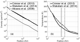
Figure 1: Radial structure of the 1D static and 0D dynamic model at final time for: (a) density, for which we plot the initial structure from Aikawa et al. (2008) as reference, (b) temperature, for which we plot the limit of the hot core (T > 100 K) for the 1D static ($R_{HC}$ = 80 AU, solid grey vertical line) and 0D dynamic ($R_{HC}$ = 135 AU, dashed grey vertical line).

3 Results

3.1 0D models

In this section we aim to do a comprehensive study of sulphur chemistry in environments such as hot cores. In particular, we want to address the importance of the temperature as well as the pre-collapse chemical composition using the four 0D simulations defined in section 2.3. Sulphur chemistry in the hot gas phase is known to be intertwined with the distribution of reactive oxygen: O, O₂ and OH (Charnley, 1997; Wakelam et al., 2004b; Esplugues et al., 2014). Hence we begin with a description of the chemistry of these species, then study the chemistry of the main S-bearing species observed towards hot and dense objects: SO, SO₂, H₂S, OCS, CS and H₂CS.

3.1.1 Oxygen chemistry

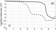
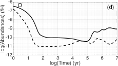
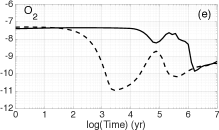
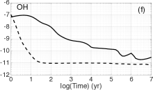
Figure 2: Abundances of O, O₂ and OH relative to H as a function of time for hot cores conditions: $n_{H}=2\times 10^{7}$ cm^-3 and T = 100 K (solid line) or 300 K (dashed line), and for LEDC (top panel) and EDC (bottom panel) pre-collapse compositions.

The left, middle and right panels of figure 2 show the abundances of respectively O, O₂ and OH, for the LEDC (top) and EDC (bottom) pre-collapse compositions. For atomic oxygen in the 0DS100LEDC case (cf figure 2 (a)), the temperature is not high enough for all the mantle of grain to evaporate and O reacts mainly with the S-bearing species available in the gas phase. It initially reacts with CS which is the second most abundant S-bearing species in the gas-phase, to form S and CO. As the abundance of CS consequently decreases, O is then mainly destroyed through formation of SO and SO₂:

$$\text{O}+\text{S${}_{2}$} \to \text{S}+\text{SO}$$ (2)

$$\text{O}+\text{SO} \to$$ SO₂ (3)

In the 0D300LEDC case (cf figure 2 (a)), the temperature of the core is high enough for mantle hydrocarbons (H_xC_n) to evaporate. They participate in the consumption of O by forming mainly CO, causing the O abundance to decrease much faster than in the 0D100LEDC case. However, the most efficient reaction at this temperature is:

$$\text{O}+\text{H${}_{2}$} \to \text{H}+\text{OH}$$ (4)

Towards the end ($t>10^{6}$ yrs), the abundance of atomic oxygen increases again from the reaction:

$$\text{CO}+\text{He${}^{+}$} \to \text{He}+\text{O}+\text{C+}$$ (5)

as well as photodissociation by secondary UV photons of SO and SO₂.
With the pre-collapse composition of the EDC, contrary to the LEDC, most of the oxygen is trapped in grain mantle, mainly under the form of H₂O, H₂CO and CO (see table 2). Hence, few atomic oxygen is available in the gas phase even after sublimation of the grain mantle, which explains that its initial abundance in both EDC cases is lower by two orders of magnitude compared to LEDC ones. In the 0DS100EDC case (cf figure 2 (d)), the temperature of the corino is hot enough to sublimate light species, especially HS and NS which are two of the sulphur reservoirs in the pre-collapse composition. These species react rapidly with O to form SO and NO for $10^{4}$ years. After this time, it is HCNS which reacts mainly with atomic oxygen through the following reactions:

$$\text{O}+\text{HCNS} \to \text{HCN}+\text{SO}$$ (6)

$$\to \text{HCO}+\text{NS}$$ (7)

The global increase of abundance of O at the end of the simulation is due to reaction (5).

In the 0D300EDC case (cf figure 2 (d)), most of the sublimated hydrocarbons efficiently form CH₃ which consumes O in the first hundred years following:

$$\text{O}+\text{CH${}_{3}$} \to \text{H}+\text{CO}+\text{H${}_{2}$}$$ (8)

$$\to \text{H}+\text{H${}_{2}$CO}$$ (9)

Afterwards, O abundance increases slowly, mainly from the reaction:

$$\text{NH}+\text{NO} \to \text{H}+\text{O}+\text{N${}_{2}$}$$ (10)

In both 0DS100LEDC and 0DS300LEDC models, dioxygen chemistry is strongly linked with S and OH chemistry via:

$$\text{S}+\text{O${}_{2}$} \to \text{O}+\text{SO}$$ (11)

$$\text{O}+\text{OH} \to \text{H}+\text{O${}_{2}$}$$ (12)

At 100 K (cf figure 2 (b)), atomic carbon initially destroys O₂ faster than it is created by reaction (12) through:

$$\text{C}+\text{O${}_{2}$} \to \text{O}+\text{CO}$$ (13)

Then, atomic sulphur consumes both O₂ and OH (cf figure 2 (c)) within a timescale of a thousand years, respectively via reaction (11) and:

$$\text{S}+\text{OH} \to \text{H}+\text{SO}$$ (14)

Afterwards, both species chemistries are linked by reaction (12). The short increase of both abundances near 10⁶ years is mainly due to the formation of OH via electronic recombination of HOCS⁺ and HSO${}_{2}^{+}$.
At 300 K however (cf figure 2 (b)), atomic carbon is initially rapidly consumed by the two evaporated hydrocarbons C₄H₂ and C₂H₂, and does not destroys O₂ as efficiently as at 100 K. Instead, OH is formed rapidly via reaction (4) (cf figure 2 (c)), which causes the O₂ abundance to increase through reaction (12) in the first hundred years. Then O₂ and OH are consumed in a few thousands years respectively by reaction (11) and:

$$\text{H${}_{2}$}+\text{OH} \to \text{H}+\text{H${}_{2}$O}$$ (15)

It should be noted that the increase in O₂ abundance near 10⁵ years is due to the following ion-neutral reactions:

$$\text{S}+\text{O${}_{2}^{+}$} \to \text{O${}_{2}$}+\text{S${}^{+}$}$$ (16)

$$\text{SO${}_{2}$}+\text{He${}^{+}$} \to \text{He}+\text{O${}_{2}$}+\text{S${}^{+}$}$$ (17)

In the EDC cases, atomic oxygen is not abundant enough in the gas phase for reaction (12) to be efficient. Hence, there is no evident link between O₂ and OH chemistries as in the LEDC cases. For the 0D100EDC model (cf figure 2 (e)), the abundance of dioxygen first slowly grow for a few hundred years from the reaction:

$$\text{HCO}+\text{O${}_{2}$H} \to \text{O${}_{2}$}+\text{H${}_{2}$CO}$$ (18)

O₂H is also destroyed by H to form OH, and when there is not enough left in the gas phase, HCO then reacts with O₂ causing its abundance to decrease after a few thousands years. Moreover, reaction (11) also becomes efficient after 10⁴ years and O₂ abundance starts to drop at this time. The increase near 10⁵ years is manly due to reaction (17).
In the 0D300EDC (cf figure 2 (e)), the CH₃ formed from the evaporated hydrocarbon destroys efficiently O₂ for a few thousands years via:

$$\text{O${}_{2}$}+\text{CH${}_{3}$} \to \text{H${}_{2}$O}+\text{HCO}$$ (19)

Afterwards, the abundance of O₂ globally increases from the following reactions:

$$\text{O${}_{3}$}+\text{S} \to \text{SO}+\text{O${}_{2}$}$$ (20)

$$\text{O${}_{2}$H}+\text{CH${}_{3}$} \to \text{CH${}_{4}$}+\text{O${}_{2}$}$$ (21)

OH abundance generally decreases in both EDC models. For the 0D100EDC case (cf figure 2 (f)), this decrease is mainly due to:

$$\text{CS}+\text{OH} \to \text{H}+\text{OCS}$$ (22)

$$\text{H${}_{2}$CO}+\text{OH} \to \text{H${}_{2}$O}+\text{HCO}$$ (23)

As for the 0D300EDC (cf figure 2 (f)), it is mainly due to reaction (15) and (23).

3.1.2 Sulphur chemistry

In the following, we take a comprehensive look at the chemistry of the main neutral S-bearing species detected in hot cores namely SO, SO₂, OCS, H₂S, H₂CS and CS.
 

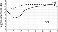
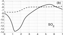
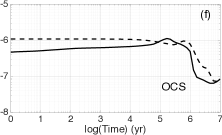
Figure 3: Abundances of SO, SO₂ and OCS relative to H as a function of time for hot cores conditions: $n_{H}=2\times 10^{7}$ cm^-3 and T = 100 K (solid line) or 300 K (dashed line), and for LEDC (top panel) and EDC (bottom panel) pre-collapse compositions.

3.1.2.1  SO, SO₂ and OCS in the LEDC cases

Figure 3 displays the abundances of SO, SO₂ et OCS in both LEDC (top panels) and EDC (bottom panels) cases. In the 0DS100LEDC case, these three species are initially destroyed by atomic carbon explaining their respective drops in the first 10 years of the simulation:

$$\text{SO}+\text{C} \to \text{S}+\text{CO}$$ (24)

$$\to \text{O}+\text{CS}$$ (25)

$$\text{SO${}_{2}$}+\text{C} \to \text{SO}+\text{CO}$$ (26)

$$\text{OCS}+\text{C} \to \text{CS}+\text{CO}$$ (27)

SO abundance then grows first mainly from reaction (14), then reactions (2) and (11) (cf figure 3 (a)). After 10⁶ years, as only a small mount of reactive oxygen remains in the gas phase, SO is no longer efficiently produced. It is instead mainly destroyed by CH through:

$$\text{SO}+\text{CH} \to \text{H}+\text{OCS}$$ (28)

$$\to \text{CO}+\text{HS}$$ (29)

SO₂ is linked with SO mainly by reaction (3), as well as:

$$\text{SO}+\text{OH} \to \text{H}+\text{SO${}_{2}$}$$ (30)

which is only efficient when OH is abundant enough in the gas phase (i.e. at the early beginning of the simulation, cf figure 2 (c)). Hence, SO₂ abundance grows from 10 to a few 10⁵ years from these reactions (cf figure 3 (b)). Afterwards, SO₂ is destroyed by H${}_{3}^{+}$ and C⁺ following:

$$\text{SO${}_{2}$}+\text{H${}_{3}^{+}$} \to \text{H${}_{2}$}+\text{HSO${}_{2}^{+}$}$$ (31)

$$\text{SO${}_{2}$}+\text{C${}^{+}$} \to \text{CO}+\text{SO${}^{+}$}$$ (32)

After his consumption by atomic carbon, OCS is also efficiently formed until 10⁵ years from HCO and HCS (cf figure 3 (c)):

$$\text{O}+\text{HCS} \to \text{H}+\text{OCS}$$ (33)

$$\text{S}+\text{HCO} \to \text{H}+\text{OCS}$$ (34)

For the remainder of the simulation, HCO⁺ is formed efficiently from reaction of H${}_{3}^{+}$ with CO, and reacts with OCS:

$$\text{OCS}+\text{HCO${}^{+}$} \to \text{CO}+\text{HOCS${}^{+}$}$$ (35)

However OCS abundance remains stable at this time because of reaction (28).

In the 0DS300LEDC case, C₄H₂ and C₂H₂ thermally desorb from grain mantle. Both these species react initially with atomic carbon with reaction rates higher of more than two orders of magnitude than those of reactions (24), (25), (26) and (27) preventing SO, SO₂ and OCS from abrupt initial consumptions. Therefore SO and SO₂ form rapidly from reactions (11), (14) and (30) (cf figure 3 (a) and (b)). When the abundance of reactive oxygen drops around 10³ years, their abundances will undergo only small variations. Indeed as the main reactions ruling SO chemistry are no longer efficient because of the lack of reactive oxygen in the gas phase, reactions that recycle SO via HSO⁺ allow its abundances to reach a quasi-static regime until the end of the simulation. For instance, due to the high temperature, high abundance of evaporated H₂O and CO render efficient the two following reactions:

$$\text{H${}_{2}$O}+\text{HSO${}^{+}$} \to \text{H${}_{3}$O${}^{+}$}+\text{SO}$$ (36)

$$\text{CO}+\text{HSO${}^{+}$} \to \text{HCO${}^{+}$}+\text{SO}$$ (37)

The SO thus formed is then put back in HSO⁺:

$$\text{SO}+\text{H${}_{3}^{+}$} \to \text{H${}_{2}$}+\text{HSO${}^{+}$}$$ (38)

As a result, SO₂ abundances shows only a small increase during the final part of the simulation, mainly due to reaction (30).
OCS abundance does not vary much in the 0DS300LEDC case (cf figure 3 (c)). When atomic oxygen is still abundant in the gas phase, OCS is mainly formed through reaction (33). Afterwards OCS is destroyed by secondary UV photons to form S and CO, and by H${}_{3}^{+}$ through:

$$\text{OCS}+\text{H${}_{3}^{+}$} \to \text{CO}+\text{HOCS${}^{+}$}$$ (39)

HOCS⁺ then recombines electronically to form either CS and OCS, which explains why the latter abundance decreases slowly.

3.1.2.2  SO, SO₂ and OCS in the EDC cases

The bottom panel of figure 3 displays the abundances of SO, SO₂ and OCS in both EDC cases. On the one hand, it appears that the chemistry of these species does not depend as much on the temperature as in the LEDC cases. This can be explained by the poor abundance of reactive oxygen, especially atomic oxygen, in the gas phase in the EDC cases compared with the LEDC cases. Table 4 displays the amount of reactive oxygen (relative to that of total oxygen) in the gas phase at the first time step of each hot core simulation. It shows that in the LEDC cases at least 33% of the total amount of oxygen is under reactive form in the gas phase, against at most 0.1% in the EDC cases.

Table 4: Description of the reactive oxygen composition in the gas phase at the first time step of the hot cores simulations (post-collapse). The values display the percentage relative to the total abundance of oxygen.

LEDC
100 K	300 K
41%	33%
EDC
100 K	300 K
0.1%	< 0.09%

On the other hand the chemistry of SO, SO₂ and OCS looks relatively inert, except for the last part of the simulation ($t>10^{5}$ years). Indeed, in the 0DS100EDC case, SO and SO₂ (cf figure 3 (d) and (e)) are at first slowly formed through reactions (14) and (30), respectively. As the abundance of HCNS grows from the evaporated NS (accumulated on the grain during the dense parent cloud phase, see table 2) through:

$$\text{NS}+\text{CH${}_{2}$} \to \text{HCNS}+\text{H}$$ (40)

the abundance of SO grows steeper from 10⁴ years thanks to reaction (6). Finally, after 10⁶ years, SO is consumed by CH through reactions (28) and (29). The strong link of SO₂ with SO via reaction (30), coupled with reaction (31), makes its abundance drops at the same time. Regarding OCS (cf figure 3 (f)), its abundance grows at first in the 0DS100EDC case from reaction (22), then from reaction (34) after 10⁴ years. Towards the end of the simulation, as for SO and SO₂, OCS is destroyed by CH via:

$$\text{OCS}+\text{CH} \to \text{H}+\text{CO}+\text{CS}$$ (41)

In the 0DS300EDC case, the chemistry of SO, SO₂ and OCS differs from the 0DS100EDC case from two main points: first, the abundance of OH decreases much faster in the 0DS300EDC case (cf figure 2 (f)), diminishing even more the quantity of reactive oxygen in the gas phase, causing the abundances of SO, SO₂ and OCS to stay relatively constant during at least the first 10⁵ years of the simulation. Secondly, CH is much less abundant at 300 K (by two to three orders of magnitude) because it is effectively destroyed by evaporated H₂O and C₂H₂:

$$\text{CH}+\text{H${}_{2}$O} \to \text{H}+\text{H${}_{2}$CO}$$ (42)

$$\text{CH}+\text{C${}_{2}$H${}_{2}$} \to \text{H}+\text{c-C${}_{3}$H${}_{2}$}$$ (43)

Hence, SO and SO₂ abundances keep on increasing at the end of the simulation (cf figure 3 (d) and (e)) and do not decrease as in the 0DS100EDC case. However, the lack of CH do not prevent the late-time decrease of OCS (cf figure 3 (f)) which is ruled by the same reactions as in the 0DS300LEDC case, namely its photodissociation by secondary UV photon and reaction (39).
 

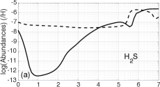
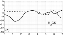
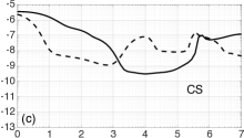
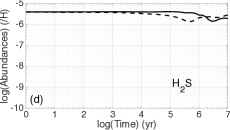
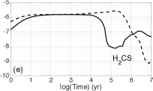
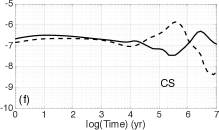
Figure 4: Abundances of H₂S, H₂CS and CS relative to H as a function of time for hot cores conditions: $n_{H}=2\times 10^{7}$ cm^-3 and T = 100 K (solid line) or 300 K (dashed line), and for LEDC (top panel) and EDC (bottom panel) pre-collapse compositions.

3.1.2.3  H₂S, H₂CS and CS in the LEDC cases

Figure 4 is the same as figure 3 but for H₂S, H₂CS and CS. In the 0DS100LEDC case, as for SO, SO₂ and OCS, H₂S and H₂CS (cf figure 4 (a) and (b)) are both initially destroyed by atomic carbon via the following reactions:

$$\text{H${}_{2}$S}+\text{C} \to \text{H}+\text{HCS}$$ (44)

$$\text{H${}_{2}$CS}+\text{C} \to \text{H}+\text{HC${}_{2}$S}$$ (45)

$$\to \text{CS}+\text{CH${}_{2}$}$$ (46)

The following increase in H₂S abundance is mainly due to two coupled reactions:

$$\text{CH${}_{2}$SH}+\text{N} \to \text{H${}_{2}$S}+\text{HCN}$$ (47)

$$\text{HCN}+\text{H${}_{3}$S${}^{+}$} \to \text{H${}_{2}$S}+\text{HCNH${}^{+}$}$$ (48)

Indeed, CH₂SH evaporates slowly from grain surface in the physical conditions of the simulation. Reacting with atomic nitrogen via reaction (47), it forms both H₂S and HCN. The latter then also forms H₂S. The combination of these two reactions explains the steep increase in H₂S abundance between 10 and 10⁵ years. Afterwards, it decreases from the following ion-neutral reactions:

$$\text{H${}_{2}$S}+\text{HCO${}^{+}$} \to \text{CO}+\text{H${}_{3}$S${}^{+}$}$$ (49)

$$\text{H${}_{2}$S}+\text{SO${}^{+}$} \to \text{H${}_{2}$O}+\text{S${}_{2}^{+}$}$$ (50)

Towards the end of the simulation, H₂S is efficiently produced by the electronic recombination of H₃S${}_{2}^{+}$, provided by the following reaction mechanism:

$$\text{S}+\text{HS}\to\text{S${}_{2}$}\xrightarrow{\text{HCO${}^{+}$}}\text{HS${}_{2}^{+}$}\xrightarrow{\text{H${}_{2}$}}\text{H${}_{3}$S${}_{2}^{+}$}$$ (51)

This mechanism is made efficient by the increase of the abundance of HS during this period of time.
H₂CS gas-phase chemistry at 100 K (in both LEDC and EDC cases, cf figure 4 (b) and (e), respectively) is intertwined with its grain chemistry because the temperature is not high enough for its complete thermal desorption from grain ices. Hence, after its destruction by atomic carbon, H₂CS grows from:

$$\text{S}+\text{CH${}_{3}$} \to \text{H${}_{2}$CS}+\text{H}$$ (52)

Then its abundance decreases from destruction by HCNH⁺ in the gas phase, as well as by hydrogenation in the grain bulk. Indeed the latter contributes to the depletion of H₂CS from the gas phase at this time because the chemistry has reached adsorption/desorption equilibrium. The reactions in question are respectively:

$$\text{H${}_{2}$CS}+\text{HCNH${}^{+}$} \to \text{H${}_{3}$CS${}^{+}$}+\text{HCN}$$ (53)

$$\text{b-H${}_{2}$CS}+\text{b-H} \to$$ b-CH₂SH (54)

where the prefix ’b-’ is for the bulk species. Afterwards, H₂CS abundance increases again, mainly from the electronic recombination of H₃CS⁺ and reaction (52).
Contrary to the other S-bearing species studied in this paper, CS is not destroyed by atomic carbon during the early phase of the simulation (cf figure 4 (c)). It is instead destroyed during a longer period of time (approximately 10⁴ years) by atomic oxygen, contributing efficiently to lock gas phase oxygen into CO via:

$$\text{CS}+\text{O} \to \text{S}+\text{CO}$$ (55)

CS abundance then grows mainly from reaction (25) as well as from the following reaction mechanism:

$$\text{S}+\text{CH${}_{2}$}\to\text{HCS}\xrightarrow{\text{S}}\text{CS${}_{2}$}\xrightarrow{\text{H}}\text{CS}$$ (56)

As previously observed, atomic carbon is preferentially consumed by evaporated hydrocarbon in the 0DS300LEDC case and therefore has a limited impact on sulphur chemistry compared to the 0DS100LEDC case. Hence, H₂S (cf figure 4 (a)) is first destroyed by atomic hydrogen and oxygen for 10³ years via:

$$\text{H${}_{2}$S}+\text{H} \to \text{H${}_{2}$}+\text{HS}$$ (57)

$$\text{H${}_{2}$S}+\text{O} \to \text{H${}_{2}$}+\text{OH}$$ (58)

H₂S is after formed by the electronic recombination of H₃S${}_{2}^{+}$ provided by a similar reaction mechanism than (51), except that instead of HCO⁺, it is the H₃O⁺ ion which mainly reacts with S₂ to form HS${}_{2}^{+}$. Indeed H₃O⁺ is much more abundant in the gas phase at 300 K than at 100 K because it comes mainly from H₂O which is totally evaporated from grain at this temperature. Furthermore, it is H₃O⁺ which destroys H₂S at the end of the simulation:

$$\text{H${}_{2}$S}+\text{H${}_{3}$O${}^{+}$} \to \text{H${}_{2}$O}+\text{H${}_{3}$S${}^{+}$}$$ (59)

At 300 K, H₂CS is fully depleted from grain surface and bulk and is affected only by gas phase chemistry (cf figure 4 (b)). Partially consumed by atomic carbon during the first 10 years, it is then formed mainly through reaction (52) and destroyed by reaction (53).
In the 0DS300LEDC case, CS is also initially destroyed by atomic oxygen via reaction (55) (cf figure 4 (c)), but for a shorter time than in the 0DS100LEDC case. The increase in its abundance at 10³ years is mostly due to a reaction mechanism starting from the evaporated C₄H₂:

$$\text{C${}_{4}$H${}_{2}$}+\text{S${}^{+}$}\to\text{HC${}_{4}$S${}^{+}$}\xrightarrow{\text{e${}^{-}$}}\text{C${}_{3}$S}\xrightarrow{\text{O}}\text{CCS}\xrightarrow{\text{S,N}}\text{CS}$$ (60)

Then CS is mainly destroyed by HCNH⁺ via:

$$\text{CS}+\text{HCNH${}^{+}$} \to \text{HCN}+\text{HCS${}^{+}$}$$ (61)

Finally, the last increase in its abundance is due to the reaction mechanism (56).
 

3.1.2.4  H₂S, H₂CS and CS in the EDC cases

In the EDC cases and prior to collapse, H₂S in icy grain bulk is the second reservoir of sulphur, containing 26% of the total amount of sulphur (see table 2). Hence its abundance in both EDC cases is generally higher than in the LEDC ones. Moreover, in the 0DS100EDC case (cf figure 4 (d)), H₂S initially forms efficiently from its abundant reservoirs counterpart HS via:

$$\text{HS}+\text{HS} \to \text{S}+\text{H${}_{2}$S}$$ (62)

It is also produced during most of the simulation from the slow evaporation of methanol, which is the fourth reservoir of oxygen in the EDC case (see table 2), and through the following reaction mechanism:

$$\text{CH${}_{3}$OH}+\text{CN}\to\text{CH${}_{2}$OH}\xrightarrow{\text{S}}\text{H${}_{2}$CO}\xrightarrow{\text{H${}_{3}$S${}^{+}$}}\text{H${}_{2}$S}$$ (63)

Towards the end, H₂S is destroyed via reaction (49).
In the 0DS100EDC case (cf figure 4 (e)), H₂CS is first formed via reaction (52) as well as from methanol slow depletion with the following reaction mechanism, similar to (63):

$$\text{CH${}_{3}$OH}+\text{CN}\to\text{CH${}_{2}$OH}\xrightarrow{\text{S}}\text{H${}_{2}$CS}$$ (64)

As in the 0DS100LEDC case, H₂CS chemistry is afterwards linked with its grain chemistry via reactions (53) and (54), making its abundance drop at 10⁵ years. At the end of the simulation H₂CS abundance increases again from reaction (52) and electronic recombination of H₃CS⁺.
Due to the small amount of reactive oxygen in the EDC cases compared to the LEDC cases (see table 4), CS is not destroyed by atomic oxygen at the beginning of the simulation (cf figure 4 (e)). At 100K, it is instead formed rapidly via:

$$\text{HCS}+\text{H} \to \text{CS}+\text{H${}_{2}$}$$ (65)

with HCS coming from the small fraction of H₂S destroyed by reaction (44). Afterward, CS is destroyed for a few 10⁵ years by OH and HS via reaction 22 and:

$$\text{CS}+\text{HS} \to \text{CS${}_{2}$}+\text{H}$$ (66)

When CS₂ abundance is high enough, it is hydrogenated back into CS, causing the abundance of the latter to grow again at the end of the simulation.

In the 0DS300EDC case, all the methanol is directly depleted in the gas phase and rapidly forms CH₃ through many different reactions. Hence, as CH₃ abundance is rapidly much higher than in the 0DS100EDC case, H₂S is mainly destroyed at 300K via (cf figure 4 (d)):

$$\text{H${}_{2}$S}+\text{CH${}_{3}$} \to \text{HS}+\text{CH${}_{4}$}$$ (67)

This high abundance of CH₃ in the gas phase also causes H₂CS to be efficiently formed for a few 10⁵ years by reaction (52) (cf figure 4 (e)). Afterwards, as in the 0DS300LEDC case, the steep decrease of its abundance is mainly due to reaction (53).
Finally, CS chemistry in the 0DS300EDC case is similar to the 0DS100EDC case, except for the fact that OH abundance at 300K is much lower than at 100K (cf figure 4 (f)). Hence, CS is mainly destroyed by reaction (66). Moreover, as CS₂ abundance grows faster at 300K than at 100K, the peak in CS abundance happens sooner in the 0DS300LEDC case. At the end, CS is destroyed like H₂CS, by HCNH⁺ via reaction (61).

3.1.3 Comparisons to observations

The species studied in this section have been detected in many hot cores and corinos, and their respective observed abundances present differences among sources that can go as high as three orders of magnitude (see for example table 5 of Wakelam et al., 2004a, and reference therein). These variations are often explained by differences among the ages of the sources, or among the temperatures of their respectives hot cores or corinos (see discussion in Herpin et al., 2009). Therefore, it would be complex, as well as out of the scope of the present study, to quantitatively compare our results to observations. Qualitatively however, we can raise the two following points:

1. The total amount of sulfur observed in massive hot cores generally account only for a small part of its cosmic abundance (around 0.1%, see Hatchell et al., 1998; van der Tak, 2004; Wakelam et al., 2004a; Herpin et al., 2009), which contrasts with our modeling results where most of the sulphur appears to be under the form of SO, SO₂, H₂S and OCS at the ages that are expected for such objects. Uncertainties on massive hot cores observations due to the fact they are mostly very distant sources, therefore not spatially resolved, as well as uncertainties on our high temperature network could explain these discrepancies. However, among this type of sources, the hot core of Orion KL presents a high abundance of H₂S of $2.5\times 10^{-6}$, accounting for more than 15% of the total mount of sulphur (Minh et al., 1990), as well as higher abundances of SO and SO₂ than in other massive hot core (Sutton et al., 1995). It appears that, even if our models fail to reproduce the observed abundances of these molecules for most massive hot cores observations, both our EDC case models can reproduce the Orion KL abundances of H₂S, SO and SO₂ within one order of magnitude in a range of time acceptable for this structure, between 10⁴ and 10⁶ years. However in this range of time, the models tend to overestimate the abundances of OCS, CS and H₂CS, which suggests that work still has to be done regarding the modelling of the chemistry of these species.
   

2. The only hot corinos towards which all the S-bearing species studied in this paper have been observed is IRAS 16293-2422. The observed abundances of SO, SO₂, OCS, H₂CS and H₂S in the dense inner part of its envelope ($\leq 150$ AU, see table 7 of Schöier et al., 2002) can be reproduced within one order of magnitude by both our LEDC case models in a range of time compatible with one derive by Schöier et al. (2002), between a few 10³ and a few 10⁴ years. This result would suggest that IRAS 16293-2422 has formed in a parent cloud that would have collapsed at an age of approximately 10⁵ years.

These results suggest that, following our previous paper (Vidal et al., 2017), our model can reproduce observations of S-bearing molecules in H₂S-rich hot cores and in hot corinos using as initial abundance of sulphur its cosmic one. However work still has to be conducted regarding our high temperature network, especially for OCS, H₂CS and CS.

3.2 1D static models

In this section we study the results of the two 1D static simulations whose parameters are described in section 2.4 and table 3. The goal is to evaluate the impact of the pre-collapse chemical composition of the parent cloud on the computed abundances of the main S-bearing species SO, SO₂, OCS, H₂S, H₂CS and CS. Both LEDC and EDC simulations were run for a period of $3.5\times 10^{5}$ years so as to make the results comparable to those of the 0D dynamic simulations presented in section 3.3.

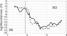
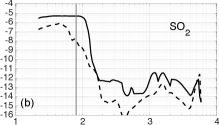
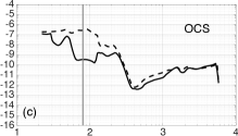
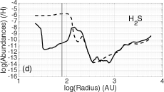
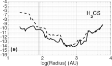
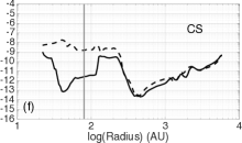
Figure 5: Abundances of SO, SO₂ and OCS (top panel) and H₂S, H₂CS and CS (bottom panel), relative to H as a function of the radius to the star IRAS 16293-2422 according to the 1D structure of Crimier et al. (2010), for the LEDC (solid line) and EDC (dashed line) pre-collapse compositions. Both models were run for a period of $3.5\times 10^{5}$ years so the results would be comparable to those of the 0D dynamic simulations. The vertical grey line represent the hot core spatial limit $R_{HC}$ = 80 AU, T > 100 K.

Figure 5 displays the abundances of each of these species for both 1DSLEDC (solid lines) and 1DSEDC (dashed lines) pre-collapse compositions. For a radius greater than 300 AU, which corresponds to the outermost and coldest (T < 50 K) part of the envelope of the protostar, most considered species present only small local differences in their abundances between the LEDC and EDC cases. Only SO₂ presents significant differences that can go to more than three orders of magnitude while other species display differences smaller than one order of magnitude (cf figure 5 (b)).

In the inner part of the envelope (R < 300 AU) where the temperature goes from 50 to 200 K (see right panel of figure 1), all species abundances show significative differences between the LEDC and EDC pre-collapse compositions. These differences can go from two to more than six orders of magnitude. Within the hot core limits (delimited by a vertical grey line in figure 5 at $R_{HC}$ < 80 AU, T > 100 K), the species which are the most sensitive to the pre-collapse composition appear to be H₂S, H₂CS, and CS with differences of more than three orders of magnitude (cf figure 5 (d), (e) and (f), respectively). For H₂S, these differences are explained by its dependance on the parent cloud evolution time. Indeed, in the EDC case, H₂S in icy grain bulk is the second reservoirs of sulphur in the pre-collapse composition, containing 26% of the total amount of sulphur, whereas in the LEDC case, it only contains 5% (see table 2). Hence, in the inner part of the envelope and the hot core, where the temperature is high enough for H₂S thermal desorption, its abundance is much higher than in the LEDC case. Moreover, figure 4 shows that in that case, H₂S is not efficiently destroyed in the gas phase. Regarding H₂CS, this species efficiently forms at high temperature in the gas phase from CH₃ (via reaction (52)) which is much more abundant in the EDC case because of evaporated methanol and hydrocarbons accumulated on grain during the parent cloud evolution. Finally, in the EDC case CS is not as efficiently destroyed in the gas phase as in the LEDC case (see figure 4) because of the low abundance of reactive oxygen (see table 4).

We can finally highlight that our 1D static models show that the pre-collapse composition of the parent cloud appears to be critical for the sulphur bearing species in hot core physical conditions. Indeed, we can see from figure 5 that a hot core that formed from a young parent cloud will be poor in H₂S and rich in SO₂, while a hot core formed from a more evolved parent cloud would be rich in H₂S and H₂CS.

3.3 0D dynamic model

In this section we carry out the same study as in the previous section but for the 0D dynamic simulations 0DDLEDC and 0DDEDC described in section 2.5 and table 3.

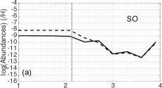
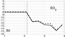
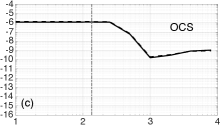
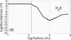
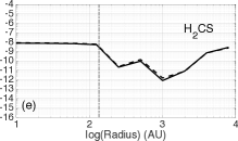
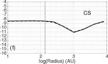
Figure 6: Abundances of SO, SO₂ and OCS (top panel) and H₂S, H₂CS and CS (bottom panel), relative to H as a function of the radius to the star IRAS 16293-2422 according to the modified structure of Aikawa et al. (2008), for the LEDC (solid line) and EDC (dashed line) pre-collapse compositions. The vertical grey dashed line represents the hot core spatial limit $R_{HC}$ = 135 AU, T > 100 K.

Figure 6 is the same as figure 5 but for the 0D dynamic simulations. What strikes directly on this figure is that the pre-collapse chemical composition of the parent cloud appears to have little or no effect on the abundances of the considered S-bearing species. Only SO presents significative difference in the hot core (delimited by a vertical grey line in figure 6 at $R_{HC}$ < 135 AU, T > 100 K), and even this difference is not of more than a factor seven (cf figure 6 (a)). A possible explanation of this lack of differences would be that the free-fall time considered in these simulations is long enough for both models to evolve towards the same chemical composition. Indeed, if the initial pre-collapse chemical composition has enough time to evolve in an environment cold enough for species not to evaporate, it will tend towards a state similar to the EDC case, i.e. with an evolved grain surface and bulk chemistry, notably with most of the sulphur transformed into H₂S and OCS on the grains. Hence, the hot core chemical composition of both 0DDLEDC and 0DDEDC would be very similar.

Moreover, the modification we made on the density profile of the model would tend to accelerate the chemistry and adsorption of species on the grains and therefore reduce the chemical timescale. We expect that by using the original model of Aikawa et al. (2008) we would get more differences and thus a more important impact of the pre-collapse chemical composition on the hot core chemistry.

4 Discussions

4.1 About the modification of the density profile of the dynamic model

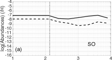
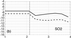
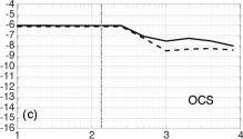
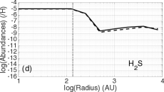
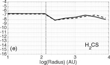
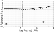
Figure 7: Abundances of SO, SO₂ and OCS (top panel) and H₂S, H₂CS and CS (bottom panel), relative to H as a function of the radius to the star IRAS 16293-2422 according to the original structure of Aikawa et al. (2008), for the LEDC (solid line) and EDC (dashed line) pre-collapse compositions. The vertical grey dashed line represents the hot core spatial limit $R_{HC}$ = 135 AU, T > 100 K.

In order to evaluate the impact of the modification of the density radial profile for our 0D dynamic model on sulphur chemistry, we run 0DDLEDC and 0DDEDC cases, but using this time the original physical structure of Aikawa et al. (2008). Figure 7 is therefore the same as figure 6, but for the models ran with the original density structure of Aikawa et al. (2008). As expected, the results displays larger differences between the LEDC and EDC pre-collapse compositions cases which can be explained by a slower chemistry due to lower density. Moreover, as discussed in Wakelam et al. (2014), lower densities tend to decrease adsorption of species on grains (and consequently depletion), and therefore enhance gas phase chemistry at low temperature, which explains why the abundances of the studied species are higher in the envelope in the original structure case. However the resulting abundances in the hot core do not change drastically (at most a bit more than one order of magnitude) and are even the same for OCS and H₂S (cf figure 7 (c) and (d), respectively). As discussed in section 3.3, this could be explained by a long free-fall time which would let the chemistry enough time for H₂S and OCS to accumulate on the grains before thermal depletion in the hot core. More complete studies of the effect of density and free-fall time on the chemistry of a collapsing envelopes and hot cores will be conducted in the future.

4.2 About H₂S and the initial abundance of sulphur

This study was conducted under the light of the last results we obtained regarding sulphur reservoir in dark clouds of Vidal et al. (2017), namely that depending on the age of the cloud, the reservoir of sulphur could either be atomic sulphur in the gas phase (LEDC case) or H₂S and HS in icy grain bulk nearly equally sharing more than 55% of the total amount of sulphur (EDC case). Another result was that the Nautilus model could reproduce the S-bearing observations in the dark cloud TMC-1 using as initial abundance of sulphur its cosmic one, or three times depleted. Hence, throughout all this paper we present results obtained using the cosmic abundance of sulphur of $1.5\times 10^{-5}$ (Jenkins, 2009). With this initial abundance of sulphur, the H₂S abundances obtained in the hot core in the dynamic simulation with the modified as well as the original structure from Aikawa et al. (2008) is as high as $10^{-5}$. Such a high abundance of H₂S is not consistent with the abundance derived from the observation of IRAS 16293-2422 ($2.7\times 10^{-7}$, see Wakelam et al., 2004a). On the one hand, to understand why the model overestimates the H₂S abundance, we ran all the models presented in this paper with an initial abundance of $5\times 10^{-6}$. It first should be noted that it only changes the presented results quantitatively, linearly diminishing the abundances of the studied species by approximately a factor three. Regarding H₂S in the dynamical case, this initial depletion of sulphur allows an estimation of its abundance in the hot core slightly overestimated around $3\times 10^{-6}$, but which could be considered in accordance with the observations (within a one order of magnitude margin).
On the other hand, the overestimation of H₂S we find could be due to the efficient formation path due to slowly evaporating CH₂SH and CH₃OH at 100 K studied in section 3.1. This is in contradiction with previous theoretical and laboratory studies that predict that in high temperature gas phase, the H₂S evaporated from grain ices is preferentially destroyed to form SO and SO₂, or molecules with two S atoms such as H₂S₂ or HS₂ (Charnley, 1997; Wakelam et al., 2004b; Druard & Wakelam, 2012; Esplugues et al., 2014; Martín-Doménech et al., 2016). Hence, this result could be a hint of missing efficient destruction gas phase reactions in the H₂S chemistry in our network.

4.3 About the sensitivity to the type of simulation

Table 5: Comparison of the abundances obtained in the LEDC case. $a(b)$ stands for $a\times 10^{b}$

Species	$(n_{i}/n_{H})_{\text{1DSLEDC}}$	$(n_{i}/n_{H})_{\text{0DDLEDC}}$
R = 50 AU (Hot core)
SO	5.7(-8)	9.0(-10)
SO2	1.4(-5)	9.5(-9)
OCS	3.0(-7)	1.2(-6)
H2S	1.2(-11)	9.5(-6)
H2CS	7.4(-10)	7.6(-9)
CS	1.2(-12)	3.3(-9)
R = 500 AU (Envelope)
SO	2.3(-14)	1.6(-10)
SO2	1.2(-13)	4.7(-12)
OCS	2.2(-12)	5.8(-8)
H2S	1.1(-13)	1.7(-10)
H2CS	2.7(-14)	1.4(-10)
CS	1.2(-13)	1.7(-10)

One goal of this article was to highlight the differences that can appear when using two types of simulations to model the same hot core. In order to do so we used a 1D static model and a 0D dynamic model of IRAS 16293-2422. Our results show that our 1D model favors a hot core sulphur chemistry dominated by SO₂ and SO in the LEDC case and H₂S in the EDC case while our 0D dynamic model displays in both cases high abundances of H₂S and OCS and low abundances of SO₂ and SO. Table 5 displays the abundances obtained for both types of models in the LEDC case, at 50 AU (in the hot core) and 500 AU (in the envelope). At the light of the difference in abundance that exists for a given species between the two type of models, one can easily conclude on the sensitivity to the type of simulation to use to compute the chemistry of a hot core and its collapsing envelope. Especially in the hot core, these differences can reach as much as six orders of magnitude, rendering critical the choice of model used to compare results with possible observations or related works.

4.4 About the importance of the pre-collapse chemical composition

The observations of S-bearing species in hot cores are still a puzzling issue, since a large variety of sulphur compositions have been observed towards different hot cores and therefore no global trend has yet been found (see figure 5 of Woods et al., 2015, and references therein). However, a given set of hot cores can present similar sulphur compositions (see for example Minh, 2016), which would suggest similar evolutionary stages. In this paper we investigated the importance of the pre-collapse chemical composition on the hot core chemistry of S-bearing species. Our results on 0D and 1D simulations (section 3.1 and 3.2) support that, given the fast evolution of sulphur chemistry in the parent cold clouds, the pre-collapse chemical composition is a critical parameter for hot core simulations. This could partially explains the absence of global trend for sulphur compositions in observed hot cores from different parent clouds, as well as supports the fact that for parent clouds collapsing at a similar ages and physical environments, hot cores can have similar sulphur compositions. However, the study of our dynamical simulation (section 3.3) raises the question of the role of the free-fall time on sulphur evolution, which would also explains similar composition for different hot cores, especially those where H₂S and OCS are found more abundant than the other species (see for example Herpin et al., 2009).

5 Conclusions

In this paper we aimed to take a comprehensive look at the chemistry of sulphur in hot cores. In order to do so, we first conducted an extensive study with simple 0D models of the chemistry of the main S-bearing species observed towards hot cores, namely SO, SO₂, OCS, H₂S, H₂CS and CS. We then presented and compared the results from two types of simulations (1D static and 0D dynamic), in order to highlight the sensitivity of chemistry to the choice of model used in astrochemical studies.

Our 0D extensive study revealed four main results:

1. The total amount of reactive oxygen in the gas phase is critically depending on the pre-collapse composition of the hot core (cf table 4) as well as the temperature;
   

2. Sulphur chemistry in hot and dense gas depends also highly on the pre-collapse composition, mainly because of its impact on reactive atomic oxygen, carbon and hydrogen, which all participate actively in most of the sulphur chemistry in such environment;
   

3. Sulphur chemistry in hot and dense gas depends highly on the temperature, partly because it is directly and indirectly linked with hydrocarbon evaporated from grain ices, and their main destruction products CH₂ and CH₃;
   

4. We found efficient paths of formation of gas phase H₂S that could be responsible for its overestimation in most of our hot core results. Studies of the gas phase chemistry of this species need to be continued to ensure the relevance of our network.

Our study of the 1D static and 0D dynamic models led to the following conclusions:

1. The pre-collapse chemical composition of the parent cloud is a key parameter for 1D static simulations of sulphur chemistry in hot cores. Indeed, the computed abundances showed that it can imply differences up to six orders of magnitude for a given species in the hot core. However, the pre-collapse composition appears to only have a small impact on the chemical composition of the envelope. Finally our 1D model shows that a hot core that was formed from a young parent cloud will be poor in H₂S and rich in SO₂, while a hot core formed from a more evolved parent cloud would be rich in H₂S and H₂CS.
   

2. The 0D dynamic simulations conducted in this paper revealed only small differences between the results of the less evolved and the evolved pre-collapse chemical composition, showing only a weak dependence of the hot core sulphur chemistry on the pre-collapse composition. Indeed, for both cases the model predicts high abundances of H₂S and OCS and low abundances of SO₂ and SO. However, this result is thought to be due to the rather long free-fall time used in our model, which would let enough time for sulphur to be adsorbed on grains and to form mainly H₂S and OCS in the envelope before thermal depletion. We expect that for a shorter free-fall time the differences between the two pre-collapse composition cases would be larger. Future work will focus on this importance of the free-fall time, since it could, along with the pre-collapse chemical composition, explain the large variety of abundances of S-bearing species observed in hot cores.

The comparison between the 1D static and 0D dynamic models displayed large differences on the computed abundances that can go as high as six orders of magnitude in the hot core. This result highlights the sensitivity to the choice of simulations in astrochemical study, especially when comparing results with observations, or with results from other paper.

References

- Aikawa et al. (2008) Aikawa Y., Wakelam V., Garrod R. T., Herbst E., 2008, ApJ, 674, 984
- Cazaux et al. (2005) Cazaux S., Caselli P., Tielens A. G. G. M., LeBourlot J., Walmsley M., 2005, in Saija R., Cecchi-Pestellini C., eds, Journal of Physics Conference Series Vol. 6, Journal of Physics Conference Series. pp 155–160 (arXiv:astro-ph/0502291), doi:10.1088/1742-6596/6/1/016
- Ceccarelli et al. (1996) Ceccarelli C., Hollenbach D. J., Tielens A. G. G. M., 1996, ApJ, 471, 400
- Chaabouni et al. (2012) Chaabouni H., Bergeron H., Baouche S., Dulieu F., Matar E., Congiu E., Gavilan L., Lemaire J. L., 2012, A&A, 538, A128
- Chang et al. (2007) Chang Q., Cuppen H. M., Herbst E., 2007, A&A, 469, 973
- Charnley (1997) Charnley S. B., 1997, ApJ, 481, 396
- Crimier et al. (2010) Crimier N., Ceccarelli C., Maret S., Bottinelli S., Caux E., Kahane C., Lis D. C., Olofsson J., 2010, A&A, 519, A65
- Druard & Wakelam (2012) Druard C., Wakelam V., 2012, MNRAS, 426, 354
- Esplugues et al. (2014) Esplugues G. B., Viti S., Goicoechea J. R., Cernicharo J., 2014, A&A, 567, A95
- Garrod & Herbst (2006) Garrod R. T., Herbst E., 2006, A&A, 457, 927
- Garrod & Pauly (2011) Garrod R. T., Pauly T., 2011, ApJ, 735, 15
- Garrod et al. (2007) Garrod R. T., Wakelam V., Herbst E., 2007, A&A, 467, 1103
- Graedel et al. (1982) Graedel T. E., Langer W. D., Frerking M. A., 1982, ApJS, 48, 321
- Harada et al. (2010) Harada N., Herbst E., Wakelam V., 2010, ApJ, 721, 1570
- Hatchell et al. (1998) Hatchell J., Thompson M. A., Millar T. J., MacDonald G. H., 1998, A&A, 338, 713
- Herbst & van Dishoeck (2009) Herbst E., van Dishoeck E. F., 2009, ARA&A, 47, 427
- Herpin et al. (2009) Herpin F., Marseille M., Wakelam V., Bontemps S., Lis D. C., 2009, A&A, 504, 853
- Hickson et al. (2016) Hickson K. M., Wakelam V., Loison J.-C., 2016, Molecular Astrophysics, 3, 1
- Hincelin et al. (2011) Hincelin U., Wakelam V., Hersant F., Guilloteau S., Loison J. C., Honvault P., Troe J., 2011, A&A, 530, A61
- Hincelin et al. (2016) Hincelin U., Commerçon B., Wakelam V., Hersant F., Guilloteau S., Herbst E., 2016, ApJ, 822, 12
- Holdship et al. (2016) Holdship J., et al., 2016, MNRAS,
- Ivezic & Elitzur (1997) Ivezic Z., Elitzur M., 1997, MNRAS, 287, 799
- Jenkins (2009) Jenkins E. B., 2009, ApJ, 700, 1299
- Karssemeijer & Cuppen (2014) Karssemeijer L. J., Cuppen H. M., 2014, A&A, 569, A107
- Kurtz et al. (2000) Kurtz S., Cesaroni R., Churchwell E., Hofner P., Walmsley C. M., 2000, Protostars and Planets IV, pp 299–326
- Loison et al. (2016) Loison J.-C., et al., 2016, MNRAS, 456, 4101
- Loison et al. (2017) Loison J.-C., et al., 2017, MNRAS, 470, 4075
- Majumdar et al. (2016) Majumdar L., Gratier P., Vidal T., Wakelam V., Loison J.-C., Hickson K. M., Caux E., 2016, MNRAS, 458, 1859
- Martín-Doménech et al. (2016) Martín-Doménech R., Jiménez-Serra I., Muñoz Caro G. M., Müller H. S. P., Occhiogrosso A., Testi L., Woods P. M., Viti S., 2016, A&A, 585, A112
- Masunaga & Inutsuka (2000) Masunaga H., Inutsuka S.-i., 2000, ApJ, 531, 350
- Minh (2016) Minh Y. C., 2016, in Journal of Physics Conference Series. p. 052007, doi:10.1088/1742-6596/728/5/052007
- Minh et al. (1990) Minh Y. C., Irvine W. M., McGonagle D., Ziurys L. M., 1990, ApJ, 360, 136
- Neufeld et al. (2005) Neufeld D. A., Wolfire M. G., Schilke P., 2005, ApJ, 628, 260
- Oya et al. (2016) Oya Y., Sakai N., López-Sepulcre A., Watanabe Y., Ceccarelli C., Lefloch B., Favre C., Yamamoto S., 2016, ApJ, 824, 88
- Podio et al. (2015) Podio L., et al., 2015, A&A, 581, A85
- Prasad & Tarafdar (1983) Prasad S. S., Tarafdar S. P., 1983, ApJ, 267, 603
- Ruaud et al. (2016) Ruaud M., Wakelam V., Hersant F., 2016, MNRAS, 459, 3756
- Sakai et al. (2014) Sakai N., et al., 2014, Nature, 507, 78
- Schöier et al. (2002) Schöier F. L., Jørgensen J. K., van Dishoeck E. F., Blake G. A., 2002, A&A, 390, 1001
- Sutton et al. (1995) Sutton E. C., Peng R., Danchi W. C., Jaminet P. A., Sandell G., Russell A. P. G., 1995, ApJS, 97, 455
- Tieftrunk et al. (1994) Tieftrunk A., Pineau des Forets G., Schilke P., Walmsley C. M., 1994, A&A, 289, 579
- Vidal et al. (2017) Vidal T. H. G., Loison J.-C., Jaziri A. Y., Ruaud M., Gratier P., Wakelam V., 2017, Monthly Notices of the Royal Astronomical Society, 469, 435
- Viti et al. (2001) Viti S., Caselli P., Hartquist T. W., Williams D. A., 2001, A&A, 370, 1017
- Wakelam & Herbst (2008) Wakelam V., Herbst E., 2008, ApJ, 680, 371
- Wakelam et al. (2004a) Wakelam V., Castets A., Ceccarelli C., Lefloch B., Caux E., Pagani L., 2004a, A&A, 413, 609
- Wakelam et al. (2004b) Wakelam V., Caselli P., Ceccarelli C., Herbst E., Castets A., 2004b, A&A, 422, 159
- Wakelam et al. (2011) Wakelam V., Hersant F., Herpin F., 2011, A&A, 529, A112
- Wakelam et al. (2014) Wakelam V., Vastel C., Aikawa Y., Coutens A., Bottinelli S., Caux E., 2014, MNRAS, 445, 2854
- Wakelam et al. (2015a) Wakelam V., et al., 2015a, ApJS, 217, 20
- Wakelam et al. (2015b) Wakelam V., Loison J.-C., Hickson K. M., Ruaud M., 2015b, MNRAS, 453, L48
- Woods et al. (2015) Woods P. M., Occhiogrosso A., Viti S., Kaňuchová Z., Palumbo M. E., Price S. D., 2015, MNRAS, 450, 1256
- van der Tak (2004) van der Tak F. F. S., 2004, in Burton M. G., Jayawardhana R., Bourke T. L., eds, IAU Symposium Vol. 221, Star Formation at High Angular Resolution. p. 59 (arXiv:astro-ph/0309152)