Tensor-network study of quantum phase transition on Sierpiński fractal

Abstract

The transverse-field Ising model on the Sierpiński fractal, which is characterized by the fractal dimension $\log_{2}^{~{}}3\approx 1.585$, is studied by a tensor-network method, the Higher-Order Tensor Renormalization Group. We analyze the ground-state energy and the spontaneous magnetization in the thermodynamic limit. The system exhibits the second-order phase transition at the critical transverse field $h_{\rm c}^{~{}}=1.865$. The critical exponents $\beta\approx 0.198$ and $\delta\approx 8.7$ are obtained. Complementary to the tensor-network method, we make use of the real-space renormalization group and improved mean-field approximations for comparison.

I Introduction

The classification of quantum phase transitions remains one of the major interests in the condensed matter physics. Although there are groups of exactly solvable models in physics, a vast majority of the physical systems calls for different approaches, in particular, for numerical calculations. Some of them are straightforwardly applicable, such as the Monte Carlo (MC) simulations, whereas the other ones, including renormalization group techniques, require development of novel algorithms.

This work is oriented for classification of the quantum phase transition on a fractal lattice, which is the infinite-size Sierpiński fractal (triangle or gasket), whose Hausdorff fractal dimension is $\log_{2}^{~{}}3\approx 1.585$. It is known that the classical Ising model exhibits no phase transition on the Sierpiński fractal Gefen et al. (1984); Luscombe and Desai (1985). Substantially less is known about its quantum counterpart. A couple of recent works investigated quantum spin models on fractals by means of real-space renormalization-group methods and by classical MC simulations Yi (2015); Kubica and Yoshida (2014); Yoshida and Kubica (2014); Wang et al. (2016); Xu et al. (2017).

In order to bring more light into the quantum fractal system, we consider a different methodology, which is the Higher-Order Tensor Renormalization Group (HOTRG) method Xie et al. (2012). It should be noted that the tensor-network viewpoint is efficient for expressing the recursive structure of the fractal lattices Genzor et al. (2016). In particular, we focus on the quantum Ising model on the Sierpiński fractal, and analyze the ground-state energy per site $E_{0}^{~{}}$ and the spontaneous magnetization $\langle\sigma^{z}_{~{}}\rangle$ with respect to the transverse field $h_{x}^{~{}}$. We first determine the critical field $h_{\rm c}^{~{}}$, and then we estimate the critical exponents $\beta$ and $\delta$ from the calculated $\langle\sigma^{z}_{~{}}\rangle$.

Structure of this article is as follows. In the next Section, we explain the lattice structure, and introduce the system Hamiltonian. We first consider two conventional calculation methods, one is the improved mean-field approximations, and the other is the real-space renormalization-group (RSRG) method. The way of applying the HOTRG method for this fractal system is presented in Sec. III. We show the numerical result in Sec. IV. Conclusions are summarized in the last section. In the Appendix, we discuss the numerical stabilization in the HOTRG method, which is realized with the correct initialization of the tensor. Two types of entanglement entropies, the vertical and the horizontal ones, of the local tensor are compared, since their ratio quantifies the anisotropy in the tensor. When they are comparable, one can avoid the instability.

II model and conventional approximations

Figure 1 shows the structure of the Sierpiński fractal. The lattice is recursively constructed by connecting three units, as shown in (a)-(d). The black dots represent the lattice sites, and the full lines represent the nearest-neighboring connections, the bonds. The $x$- and $y$-axes are used to denote the two-dimensional plane on which the fractal is located. The $x$-axis is parallel to the bonds denoted by $i$, whereas the $y$-axis is not parallel to $j$. The $z$-axis is perpendicular to the plane. For the moment, let us omit the vertical (dotted) lines and disregard the tensor notations shown in the figure.

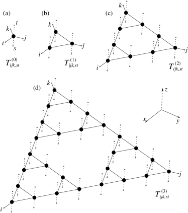
Figure 1: Structure of the Sierpiński fractal. (a) The smallest unit consists of a site shown by the black circle, from which the three bonds $i$, $j$, and $k$ emerge. (b)-(d) Connecting the three units, one can iteratively expand the size of the unit. The vertical dotted lines correspond to the imaginary-time evolution, which is considered in Sec. III.

The Hamiltonian of the transverse-field Ising model on the lattice has the form

$$H=-J\sum_{\langle a,b\rangle}^{~{}}\sigma^{z}_{a}\sigma^{z}_{b}-h_{x}^{~{}}\sum_{a}^{~{}}\sigma^{x}_{a}-h_{z}^{~{}}\sum_{a}^{~{}}\sigma^{z}_{a}\,,$$ (1)

where $\sigma^{x}_{a}$ and $\sigma^{z}_{a}$ represent the Pauli spin operators acting on the lattice site $a$. The uniform fields $h_{x}^{~{}}$ and $h_{z}^{~{}}$, respectively, are applied to the transverse ($x$-) and longitudinal ($z$-) directions. The ferromagnetic Ising interaction $J>0$ is present between the nearest-neighboring spin pairs $\sigma^{z}_{a}$ and $\sigma^{z}_{b}$. The interacting pairs are denoted by the symbol $\langle a,b\rangle$, and they are located on bonds in the fractal lattice. Throughout this article we focus on the ground-state of this system and its quantum phase transition with respect to the transverse field $h_{x}^{~{}}$. Hereafter we assume $J=1$. The parameter $h_{z}^{~{}}$ is set to zero unless its value is specified.

Before we start explaining the details of the HOTRG method, we briefly introduce the two conventional approximation schemes. The first one is the mean-field approximation, which offers a rough insight into the ground-state. We consider three types of the gradually improving mean-field approximations, beginning from the smallest unit size shown in Fig. 1(a), followed by an extended unit size with the 3 sites in Fig. 1(b), and finally that with the 9 sites in Fig. 1(c). All of the interactions inside each extended unit are treated rigorously while the inter-unit Ising interaction through the bonds $i$, $j$, and $k$ are replaced by the mean-field value $-J\langle\sigma_{~{}}^{z}\rangle$. Here, the average of the bond energy and magnetization is taken over all the sites in the extended unit. Thermodynamic functions could be estimated with a better precision if the size of the unit gets larger. We confirm this conjecture in Sec. IV.

The second approximation scheme we consider is the conventional real-space renormalization group (RSRG) method Wilson (1975), which shares some aspects in common with the HOTRG method. The RSRG method consists of an iterative procedure, where the effective intra-unit Hamiltonian $H^{(\ell)}_{a}$ for $\ell=0,1,2,\dots$ is created recursively. (The expanded unit contains $3^{\ell}_{~{}}$ sites.) Since we intend to estimate the critical field $h_{\rm c}^{~{}}$ only, we explain the case when $h_{z}^{~{}}=0$. At the initial step, which corresponds to the single site in Fig. 1(a), we have $H^{(0)}_{a}=-h_{x}^{~{}}\,\sigma_{a}^{x}$ and the spin operators $\sigma_{a;i}^{(0)}=\sigma_{a;j}^{(0)}=\sigma_{a;k}^{(0)}=\sigma_{a}^{z}$, where $a$ specifies the site location, and $i$, $j$, $k$ denote the pairing directions of the neighboring interactions.

Let us consider the 3-site extended unit shown in Fig. 1(b), and label the sites as $a$ (left), $b$ (right), and $c$ (top). The Hamiltonian of this 3-site unit is then written as

$${\cal H}^{(\ell)}_{~{}} = H_{a}^{(\ell)}+H_{b}^{(\ell)}+H_{c}^{(\ell)}$$ (2)

$$- \sigma^{(\ell)}_{a;j}\sigma^{(\ell)}_{b;i}-\sigma^{(\ell)}_{b;k}\sigma^{(\ell)}_{c;j}-\sigma^{(\ell)}_{c;i}\sigma^{(\ell)}_{a;k}$$

at the initial iteration step $\ell=0$. After diagonalizing ${\cal H}^{(\ell)}_{~{}}$, we keep only those eigenstates that are associated with $D$ lowest eigenvalues (while the remaining high-energy eigenstates are discarded). The renormalization group transformation $U$ is then chosen to the projection to the low-energy eigenstates, which reduce the dimension down to $D$. Applying $U$ to ${\cal H}^{(\ell)}_{~{}}$, we obtain the renormalized intra-unit Hamiltonian

$$H^{(\ell+1)}_{\chi}=U^{\dagger}_{~{}}{\cal H}^{(\ell)}_{~{}}\,U_{~{}}$$ (3)

for the extended unit labeled by $\ell+1$, where $\chi=a,b,c$ is the site index for the extended unit. In the same manner, we obtain the renormalized $z$-component of the spin

$$\sigma^{(\ell+1)}_{a;i} = U^{\dagger}_{~{}}\sigma^{(\ell)}_{a;i}\,U_{~{}},$$

$$\sigma^{(\ell+1)}_{b;j} = U^{\dagger}_{~{}}\sigma^{(\ell)}_{b;j}\,U_{~{}},$$

$$\sigma^{(\ell+1)}_{c;k} = U^{\dagger}_{~{}}\sigma^{(\ell)}_{c;k}\,U_{~{}},$$ (4)

at each corner of the extended unit. At this point, we can return to Eq. (2) to obtain an effective Hamiltonian ${\cal H}^{(\ell+1)}_{~{}}$ for the 9-site unit shown in Fig. 1(c). As we show in Sec. IV, the transition point (the critical phase transition field) is obtained with relatively high numerical precision if a sufficiently large $D$, the number of the block-spin state, is taken.

III Higher-Order Tensor Renormalization Group

We focus on the numerical analysis of the quantum fractal system by means of the HOTRG method Xie et al. (2012), which has yielded a high numerical accuracy for two- and three-dimensional classical Ising model. The method has also been applied to one- and two-dimensional quantum Ising model through the quantum-classical correspondence, which is a discrete imaginary-time path-integral representation. The imaginary-time evolution expressed by the density operator $\rho=e^{-\tau{\cal H}}_{~{}}$ is essential, as it behaves as the projection to the ground-state in the large $\tau$ limit.

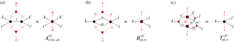
Figure 2: (Color online) Graphical representation of the processes in the HOTRG method in Eqs. (13a)-(13c). We use the large symbols to indicate the tensors $T^{(\ell)}_{~{}}$ (circles), $A^{(\ell)}_{~{}}$ (diamonds), $B^{(\ell)}_{~{}}$ (squares), and the projectors $U$, $U^{\prime}$, and $U^{\prime\prime}$ (triangles).

Let us consider the Hamiltonian in Eq. (1) and divide the imaginary-time span $\tau$ into $m$ intervals $\Delta\tau=\tau/m$. We express $\rho$ in the form of product

$$\rho=\left(e^{-\Delta\tau{\cal H}}_{~{}}\right)^{m}_{~{}}=\left[e^{-\Delta\tau\left({\cal H}_{zz}^{~{}}+{\cal H}_{x}^{~{}}+{\cal H}_{z}^{~{}}\right)}_{~{}}\right]^{m}_{~{}}$$ (5)

among imaginary-time intervals, where ${\cal H}_{zz}^{~{}}$, ${\cal H}_{x}^{~{}}$, and ${\cal H}_{z}^{~{}}$, respectively, correspond to the first, second, and third term in the r.h.s. of Eq. (1). Although ${\cal H}_{x}^{~{}}$ does not commute with ${\cal H}_{zz}^{~{}}$ or ${\cal H}_{z}^{~{}}$, a good approximation of $\rho$ can be obtained by means of the Trotter-Suzuki decomposition Trotter (1959)

$$\rho\approx\left[e^{-\Delta\tau\left({\cal H}_{zz}^{~{}}+{\cal H}_{z}^{~{}}\right)}_{~{}}\,e^{-\Delta\tau{\cal H}_{x}^{~{}}}_{~{}}\right]^{m}_{~{}}\,,$$ (6)

provided that $\Delta\tau$ is sufficiently small (e.g. $\Delta\tau\approx 0.01$). Each imaginary-time interval, which corresponds to $e^{-\Delta\tau{\cal H}}_{~{}}$, plays the role of the transfer matrix.

Applying a duality transformation, which introduces new two-state variables in the middle of the connected bonds, we can express the transfer matrix in terms of the tensor network. Figure 1 shows the structure of the transfer matrix for the elementary unit, in (a) and for the extended ones, in (b)-(d). This time, we regard the black dots as local tensors, which have three legs in the spatial direction shown by the lines, and two legs in the imaginary-time directions shown by the vertical dotted lines. Each local tensor is given by

$$T^{(0)}_{ijk,st}=\sum_{\sigma}^{~{}}W_{\sigma i}^{~{}}W_{\sigma j}^{~{}}W_{\sigma k}^{~{}}P_{\sigma s}^{~{}}P_{\sigma t}^{~{}}G_{\sigma}^{~{}}\,,$$ (7)

where the matrix

$$W=\left(\begin{array}[]{rr}\sqrt{\cosh(J\Delta\tau)}&\sqrt{\sinh(J\Delta\tau)}\\[1.42262pt] \sqrt{\cosh(J\Delta\tau)}&-\sqrt{\sinh(J\Delta\tau)}\end{array}\right)$$ (8)

originates from the Ising interaction in ${\cal H}_{zz}^{~{}}$ between the neighboring spins. The other matrix

$$P=\frac{1}{\sqrt{2}}\left(\begin{array}[]{rr}\exp(h_{x}^{~{}}\Delta\tau/2)&\exp(-h_{x}^{~{}}\Delta\tau/2)\\[1.42262pt] \exp(h_{x}^{~{}}\Delta\tau/2)&-\exp(-h_{x}^{~{}}\Delta\tau/2)\end{array}\right)$$ (9)

corresponds to the spin-flipping effect by the transverse field $h_{x}^{~{}}$ in ${\cal H}_{x}^{~{}}$, and the column vector

$$G=\left(\begin{array}[]{c}\exp(\phantom{+}h_{z}^{~{}}\Delta\tau)\\[1.42262pt] \exp(-h_{z}^{~{}}\Delta\tau)\end{array}\right)$$ (10)

represents the effect of external field $h_{z}^{~{}}$ along the z-direction in ${\cal H}_{z}^{~{}}$. All the indices $i$, $j$, $k$, $s$, and $t$ of $T^{(0)}_{ijk,st}$ thus carry two degrees of the freedom.

The transfer matrices $T^{(1)}_{ijk,st}$, $T^{(2)}_{ijk,st}$, and $T^{(3)}_{ijk,st}$ for the extended units, respectively, shown in Fig. 1(b), (c), and (d), can be obtained by contracting horizontal legs in a recursive manner. Actually, we do not directly treat these extended transfer matrices. Our aim is to obtain the local thermodynamic quantities

$$\langle O\rangle=\frac{{\rm Tr}\,\left(\,O\rho\,\right)}{{\rm Tr}~{}(\rho)}=\frac{{\rm Tr}\,\left(\,O\,e^{-\tau{\cal H}}_{~{}}\,\right)}{{\rm Tr}~{}\left(e^{-\tau{\cal H}}_{~{}}\right)}\,,$$ (11)

where $O$ represent a local operator, for a sufficiently wide system when $\tau$ is large enough. For this purpose, we do not have to construct $\rho$ in a faithful manner, but only need to consider a series of finite-size clusters represented as a stack of the extended transfer matrices, i.e.,

$$\left[T^{(1)}_{ijk,st}\right]^{2},\left[T^{(2)}_{ijk,st}\right]^{4},\left[T^{(3)}_{ijk,st}\right]^{8},\dots,\left[T^{(\ell)}_{ijk,st}\right]^{2^{\ell}},\dots$$

By use of these tensors and another series of tensors that contain the operator $O$ inside, the following ratio

$$\lim_{\tau\rightarrow\infty}^{~{}}\,\frac{\langle\phi|\,e^{-\tau{\cal H}/2}_{~{}}\,O\,e^{-\tau{\cal H}/2}_{~{}}|\phi\rangle}{\langle\phi|\,e^{-\tau{\cal H}/2}_{~{}}~{}e^{-\tau{\cal H}/2}_{~{}}|\phi\rangle}$$ (12)

can be obtained, which coincides with $\langle O\rangle$ in Eq. (11) for a wide choice of the boundary conditions and the trial state represented by $|\phi\rangle$. The HOTRG method is appropriate for this purpose. Alternatively, the value in Eq. (12) can be obtained by use of tensor product state Nishino et al. (2001); Gendiar et al. (2003) and also the projected entangled pair state Verstraete and Cirac (2004), but the computational cost is much higher.

We create the stack of the transfer matrices in a renormalized form, through the recursive contraction processes,

$$A_{ii^{\prime}kk^{\prime},ab}^{(\ell)}=\sum_{jss^{\prime}tt^{\prime}}^{~{}}T^{(\ell)}_{ijk,st}\,T^{(\ell)}_{ji^{\prime}k^{\prime},s^{\prime}t^{\prime}}\,U_{ss^{\prime},a}^{~{}}\,U_{tt^{\prime},b}^{~{}}\,,$$ (13a)

$$B^{(\ell)}_{ijk,st}=\sum_{\genfrac{}{}{0.0pt}{}{mn}{aa^{\prime}bb^{\prime}}}A_{ijmn,ab}^{(\ell)}\,T^{(\ell)}_{knm,a^{\prime}b^{\prime}}\,U^{\prime}_{aa^{\prime},s}\,U^{\prime}_{bb^{\prime},t}\,,$$ (13b)

$$T^{(\ell+1)}_{ijk,st}=\sum_{\genfrac{}{}{0.0pt}{}{umm^{\prime}}{nn^{\prime}oo^{\prime}}}B^{(\ell)}_{mno,su}B^{(\ell)}_{m^{\prime}n^{\prime}o^{\prime},ut}U^{\prime\prime}_{mm^{\prime},i}U^{\prime\prime}_{nn^{\prime},j}U^{\prime\prime}_{oo^{\prime},k}\,.$$ (13c)

which are depicted by diagrams in Fig. 2. The projectors $U$, $U^{\prime}$, and $U^{\prime\prime}$, which are also called as isometries, are quasi unitary rectangular matrices of the size $D^{2}\times D$, with $D$ being the degree of the freedom for a tensor index. These matrices are obtained from the higher-order singular value decomposition, whenever two tensors are combined and consequently reshaped into a matrix form Xie et al. (2012). We keep the states that correspond to $D$ largest singular values. Hence, the larger the $D$, the better the approximation is Genzor et al. (2016); de Lathauwer et al. (2000). The expansion procedure is stopped after all of the thermodynamic functions (normalized per site) completely converge.

In this manner the HOTRG method, applied to the discrete path-integral representation of the quantum fractal system, enables us to built up a sufficiently large finite-size system. Note that during the recursive extension of the system, we can obtain thermodynamic functions such as the ground-state energy $E_{0}^{~{}}$ per site, as it is has been done for transverse-field Ising model on the square lattice. Further details on the calculation of $E_{0}^{~{}}$ can be found in Refs. Xie et al., 2012; Genzor et al., 2016. One-point functions, such as magnetization $\langle\sigma^{z}\rangle$, can also be calculated by introducing an impurity tensor, as discussed in Ref. Genzor et al., 2016. In the appendix we discuss the choice of $\Delta\tau$ and the stabilization of numerical calculation by means of an appropriate choice of the initial tensor.

IV Numerical results

The mean-field approximation (MFA) offers a rough insight into phase transitions. As we have introduced in Sec. II, we consider series of the three approximations, MFA${}_{1}^{~{}}$, MFA${}_{3}^{~{}}$, and MFA${}_{9}^{~{}}$, respectively, where the interactions inside the (extended) units shown in Fig. 1 (a), (b), and (c) are treated exactly. We have also introduced the RSRG method, which can capture critical behavior of the model, provided that a sufficiently large number of the block-spin states $D$ is kept. However, the improvement in expectation values with respect to $D$ is rather slow. In contrast, the numerical precision in the HOTRG method significantly improves with $D$. We have confirmed that $D=8$ is large enough to obtain well-converged results on this fractal lattice. We present the numerical results up to $D=20$ in the HOTRG method.

We first compare the three types of mean-field approximations with the HOTRG method when $D=8$. The ground-state energy per site $E_{0}^{~{}}$ with respect to the transverse field $h_{x}^{~{}}$ is shown in Fig. 3. The ground-state energy obtained by the HOTRG method is always the lower than those obtained by the mean-field approximations. This can be better visible by comparing $E_{0}^{~{}}$ around the phase transition $h_{x}^{~{}}=h_{\rm c}^{~{}}$ as shown in the top inset. The bottom inset shows the spontaneous magnetization $\langle\sigma^{z}_{~{}}\rangle$. Since the fractal lattice is not homogeneous, the expectation value is calculated by averaging three independent impurity operators Genzor et al. (2017) contained in $T^{(1)}$, cf Fig. 1(b). From $\langle\sigma^{z}_{~{}}\rangle$ obtained by the HOTRG method, the critical field is determined as $h_{\rm c}^{~{}}=1.865$.

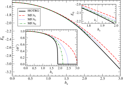
Figure 3: (Color online) The ground-state energy per site $E_{0}^{~{}}$ versus transverse field $h_{x}^{~{}}$ at $h_{z}^{~{}}=0$. The data obtained by the HOTRG method are shown by the thick full lines. The mean-field approximations MFA${}_{1}^{~{}}$, MFA${}_{3}^{~{}}$, and MFA${}_{9}^{~{}}$ are, respectively, shown by dashed, dotted, and dot-dashed lines. The top inset shows $E_{0}^{~{}}$ around the transition point $h_{\rm c}^{~{}}$. The bottom inset shows $\langle\sigma^{z}_{~{}}\rangle$.

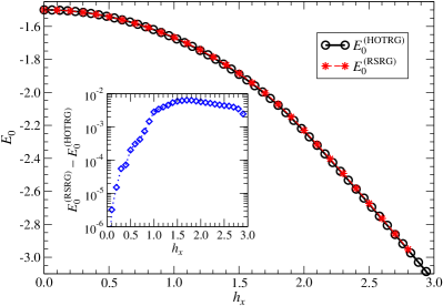
Figure 4: (Color online) The ground-state energies per site with respect to $h_{x}^{~{}}$ calculated by the HOTRG method ($D=8$) and by the RSRG method ($D=24$) when $h_{z}^{~{}}=0$. The inset shows their difference.

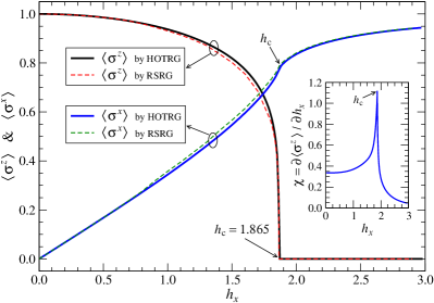
Figure 5: (Color online) Spontaneous magnetization $\langle\sigma^{z}\rangle$ and the induced polarization $\langle\sigma^{x}\rangle$ with respect to $h_{x}^{~{}}$. The full lines show the calculated result by the HOTRG method ($D=8$) and the dashed ones by the RSRG method ($D=24$). The inset shows the susceptibility $\chi$ defined by Eq. (15).

The RSRG method provides relatively accurate $E_{0}^{~{}}$ when $D=24$ block-spin states are kept. Figure 4 shows $E_{0}^{~{}}$ obtained by the RSRG method ($D=24$) and that by the HOTRG method ($D=8$). The inset shows the difference in the calculated $E_{0}^{~{}}$, within the range $0\leq h_{x}^{~{}}\leq 3$, which is not conspicuous. Figure 5 shows the spontaneous magnetization $\langle\sigma^{z}_{~{}}\rangle$ and induced polarization $\langle\sigma^{x}_{~{}}\rangle$. The difference between both of the methods is better visible below the transition point. The spontaneous magnetization $\langle\sigma^{z}_{~{}}\rangle$ by the RSRG method gives the critical field $h_{\rm c}^{~{}}=1.864$, which is close to the value $h_{\rm c}^{~{}}=1.865$ determined by the HOTRG method. The induced polarization $\langle\sigma^{x}_{~{}}\rangle$ is calculated by making use of the Hellman-Feynman theorem Feynman (1939)

$$\langle\sigma^{x}_{~{}}\rangle=-\frac{\partial E_{0}}{\partial h_{x}}\,,$$ (14)

which exhibits a weak singularity at the critical field $h_{x}^{~{}}=h_{\rm c}^{~{}}$, as marked by the arrow. (We still consider the case $h_{z}^{~{}}=0$.) The inset of Fig. 5 shows the susceptibility

$$\chi=-\frac{\partial^{2}E_{0}^{~{}}}{\partial h_{x}^{2}}=\frac{\partial\langle\sigma^{x}_{~{}}\rangle}{\partial h_{x}^{~{}}}\,$$ (15)

for the result of the HOTRG method, where there is a singular peak at $h_{\rm c}^{~{}}$.

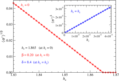
Figure 6: (Color online) Linear behavior in $\langle\sigma^{z}\rangle^{1/0.20}$ below $h_{\rm c}^{~{}}$, which means $\beta=0.20$. The inset shows linear behavior in $\langle\sigma^{z}\rangle^{8.7}$ with respect to the longitudinal field $h_{z}^{~{}}\to 0$ at the criticality $h_{x}^{~{}}=h_{\rm c}^{~{}}$; the linear behavior occurs at $\delta=8.7$. These values are obtained by the HOTRG method at $D=20$.

Finally, we increase $D$ in the HOTRG method to $D=20$, which is still computationally feasible, in order to determine the critical field $h_{\rm c}^{~{}}$ and the critical exponents $\beta$ and $\delta$ precisely. The exponent $\beta$ is associated with the critical behavior of the spontaneous magnetization $\langle\sigma^{z}_{~{}}\rangle\propto(h_{\rm c}^{~{}}-h_{x}^{~{}})^{\beta}_{~{}}$. Assuming the scaling form and applying the least-square fitting to the calculated $\langle\sigma^{z}\rangle$, we obtain $h_{\rm c}^{~{}}=1.865$ and $\beta=0.20$. For confirmation, we plot $\langle\sigma^{z}_{~{}}\rangle^{1/\beta}_{~{}}$ with $\beta=0.20$ in Fig. 6, where the linear behavior below $h_{\rm c}^{~{}}$ is evident. The other exponent $\delta$ is associated with the scaling $\langle\sigma^{z}_{~{}}\rangle\propto h_{z}^{1/\delta}$ at the critical field $h_{x}^{~{}}=h_{\rm c}^{~{}}$. In the inset, we show $\langle\sigma^{z}_{~{}}\rangle^{\delta}$ with respect to $h_{z}^{~{}}$, which is linear if we assume $\delta=8.7$.

V Summary

The transverse-field Ising model on the Sierpiński fractal was studied by the three methods: (1) the mean-field approximation, (2) the RSRG method, which can be easily adapted for the fractal structure, and (3) the HOTRG method, which had reproduced very reliable results for the transverse-field Ising model on the square lattice Xie et al. (2012). The numerical algorithm in the original HOTRG method has been generalized in order to contract a tensor network with the fractal structure. We performed the entanglement-entropy analysis in the HOTRG method at the initial stage, in order to stabilize the numerical calculation, as shown in the Appendix.

We have confirmed the existence of the second-order phase transition in the quantum Ising model on the Sierpiński fractal, whose Hausdorff dimension $d_{\rm H}^{~{}}\approx 1.585$. The critical field is $h_{\rm c}^{~{}}=1.865$, and the two critical exponents $\beta=0.20$ and $\delta=8.7$ are obtained. Our results are in a good agreement with the MC simulations by Yi Yi (2015), which resulted in $h_{\rm c}^{~{}}=1.865(2)$ and $\beta=0.19(2)$. Table 1 summarizes the transition point $h_{\rm c}^{~{}}$ and the exponents $\beta$ and $\delta$ for the transverse-field Ising model on the chain, the Sierpiński fractal, and the square lattice.

Table 1: Comparison of $h_{\rm c}^{~{}}$, $\beta$, and $\delta$ for the transverse-field Ising model on the chain ($d_{\rm H}^{~{}}=1$), the Sierpiński fractal ($d_{\rm H}^{~{}}=\log_{2}3$) Yi (2015), and the square lattice ($d_{\rm H}^{~{}}=2$) Xie et al. (2012); Kolesik and Suzuki (1994).

$d_{\rm H}$	$h_{\rm c}^{~{}}$	$\beta$	$\delta$	method used
$\log_{2}2=1\hfill$	1.0000	0.1250	15	exact solution
$\log_{2}3\approx 1.585$	1.8650	0.2000	8.7	MC, HOTRG
$\log_{2}4=2\hfill$	3.0439	0.3295	4.8	CAM, HOTRG

Relation between critical behavior and the fractional dimensionality has not been fully investigated yet, and there are open problems to be considered. One of them is the classification of the quantum phase transition on the fractal lattice with $d_{\rm H}^{~{}}=\log_{4}12$ that was recently studied for the classical system Genzor et al. (2016). This particular fractal can be dealt with the HOTRG method, as we have considered. It is also possible to generate a set of fractal lattices, which have the Hausdorff dimensions $1<d_{\rm H}<2$, as extensions. How does the the hyper-scaling relations look like on fractal lattices?

Recent studies on neural networks Amin et al. (2016); Biamonte et al. (2017) have some aspects in common with the current study, in the point that the formation of complex network geometry is required. Investigations of the quantum phase transitions on such non-typical lattices could be of use for the initial parameterization of the neural networks with complex geometry. So far, in the field of tensor-network, supervised machine learning Stoudenmire and Schwab (2016) and quantum machine learning Huggins et al. (2018) were performed on regular lattices. We conjecture that tensor networks with fractal structure, such as the tree tensor network, could lead to an efficient approximation of a given probability distribution in machine learning.

*

Appendix A Remarks on initialization

It is known that the Trotter-Suzuki decomposition in Eq. (6) introduces an error of the order of $(\Delta\tau)^{2}_{~{}}$. Thus it is more suitable to keep $\Delta\tau$ relatively small. We choose $\Delta\tau$ of the order $10^{-2}$ in most of the numerical calculations. When $\Delta\tau$ is too small, however, there is a conspicuous anisotropy between the space and imaginary-time directions. A naive application of the iterative processes in Eqs. (13a)-(13c) can cause numerical instabilities, especially, near the critical field $h_{c}$. This occurs when $\Delta\tau$ is very small, because the local tensor $T^{(0)}_{~{}}$ works as an identity in the imaginary time direction, and this situation requires to keep huge $D$ in the vertical direction, which is not feasible for realistic computational resources.

In order to avoid the instability, we modify the definition of the initial tensor $T_{ijk,st}^{(0)}$ by implementing the “vertical stacking” of the original local tensor, before we start the main iterations in Eqs. (13a)-(13c). As we explain here, the succeeding stacking process, which is followed by the renormalization-group transformation, gradually makes the local tensor isotropic. We introduce two quantities, the planer and the vertical entanglement entropies. Identifying all the tensor element as a kind of quantum wave function, it is understood that the relation between these two entanglement entropies quantifies the anisotropy in the initial tensor.

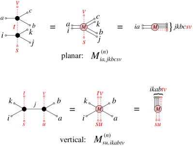
Figure 7: (Color online) Graphical representations of Eqs. (17) and (21) with the planar (top) and the vertical (bottom) constructions of the $M$ tensors, respectively. These tensors can be interpreted as rectangular matrices of the size $D^{2}\times 2^{2}D^{4}$ (top) and $2^{2}\times 2^{2}D^{4}$ (bottom), respectively, and the singular value decomposition in Eqs. (18) and (22) is applied.

Let us introduce a new notation $T^{(0,n)}_{~{}}$, where the integer $n=0,1,2,\dots$ enumerates the number of the stacking processes. The first one $T^{(0,n=0)}_{~{}}$ is the original local tensor, whose element is the $T_{ijk,st}^{(0)}$ in Eq. (7). The tensor $T^{(0,n+1)}_{~{}}$ is obtained recursively by stacking two $T^{(0,n)}_{~{}}$ vertically and performing the contraction

$$T^{(0,n+1)}_{ijk,st}=\sum_{\genfrac{}{}{0.0pt}{}{abcd}{efu}}^{~{}}T^{(0,n)}_{abc,su}\,T^{(0,n)}_{def,ut}\,U^{(n)}_{ad,i}\,U^{(n)}_{be,j}\,,U^{(n)}_{cf,k}\,,$$ (16)

which is essentially the same as Eq. (13c). Figure 2(c) shows the graphical representation of this process. The isometry $U^{(n)}_{~{}}$ is obtained as follows. We first combine the two identical tensors $T^{(0,n)}_{~{}}$ vertically

$$M^{(n)}_{ia,jkbcsv}=\sum_{t=1}^{D}T^{(0,n)}_{ijk,st}\,T^{(0,n)}_{abc,tv}\,,$$ (17)

as shown in the graphical representation in Fig. 7 (top). We perform the singular value decomposition de Lathauwer et al. (2000) (SVD) that factorizes $M^{(n)}_{~{}}$ as

$$M^{(n)}_{ia,jkbsv}=\sum_{\xi=1}^{D^{2}_{~{}}}U^{(n)}_{ia,\xi}\,\,\omega^{(n)}_{\xi}\,V^{(n)}_{\xi,jkbsv}\,.$$ (18)

This SVD specifies the isometry $U^{(n)}_{~{}}$ we need in Eq. (16). It should be noted that the singular values $\omega^{(n)}_{\xi}\geq 0$ plays an important role in both the renormalization-group transformation and the determination of the entanglement entropy. In the contraction with $U^{(n)}_{~{}}$, we keep $D$ largest singular values from $D^{2}_{~{}}$ ones, and discard the rest of them. One finds that $T^{(0,n)}_{~{}}$ corresponds to the stack of $2^{n}_{~{}}$ numbers of $T^{(0,0)}_{~{}}$, which is contracted by the tree-tensor network constructed by $U^{(m)}_{~{}}$ for $m=0$ up to $m=n-1$.

Let us identify $M^{(n)}_{ia,jkbsv}$ in Eq. (A.2) as a kind of another quantum wave function $\Psi_{ia,jkbsv}^{~{}}$ in order to define the planar entanglement entropy

$$\varepsilon^{(n)}_{\rm planar}=-\sum_{\xi=1}^{D^{2}}\frac{\left[\omega^{(n)}_{\xi}\right]^{2}_{~{}}}{\Omega_{n}}\ln\frac{\left[\omega^{(n)}_{\xi}\right]^{2}_{~{}}}{\Omega_{n}}$$ (19)

for the division of the index into $ia$ and $jkbsv$, where we have used the normalization

$$\Omega_{n}=\sum_{\xi=1}^{D^{2}}\left[\omega^{(n)}_{\xi}\right]^{2}_{~{}}$$ (20)

for the probability. The entanglement entropy $\varepsilon^{(n)}_{\rm planar}$ quantifies how strongly the part of the ‘quantum’ system, specified by the indices $ia$, is correlated with the rest of the system, as specified by the indices $jkbsv$, cf Eq. (18). (It should be noted that the planer entanglement entropy $\varepsilon^{(n)}_{\rm planar}$ is obtained after stacking $T^{(0,n)}_{~{}}$ vertically.)

A way of quantifying the anisotropy in $T^{(0,n)}_{~{}}$ is to observe the entanglement entropy in the vertical direction. Figure 7 (bottom) shows the horizontal contraction between the two $T^{(0,n)}_{~{}}$

$${\tilde{M}}^{(n)}_{su,ikabtv}=\sum_{j}^{~{}}\,T^{(0,n)}_{ijk,st}\,T^{(0,n)}_{jab,uv}\,.$$ (21)

Performing the singular value decomposition,

$${\tilde{M}}^{(n)}_{su,ikabtv}=\sum_{\xi=1}^{2^{2}_{~{}}}{\tilde{U}}^{(n)}_{su,\xi}\,\,{\tilde{\omega}}^{(n)}_{\xi}\,{\tilde{V}}^{(n)}_{\xi,ikabtv}\,,$$ (22)

we obtain the singular values ${\tilde{\omega}}^{(n)}_{\xi}$. Identifying ${\tilde{M}}^{(n)}_{su,ikabtv}$ as a kind of quantum wave function $\Phi_{su,ikabtv}^{~{}}$, we obtain the vertical entanglement entropy

$$\varepsilon^{(n)}_{\rm vertical}=-\sum_{\xi=1}^{2^{2}_{~{}}}\frac{\left[{\tilde{\omega}}^{(n)}_{\xi}\right]^{2}_{~{}}}{\tilde{\Omega}_{n}}\,\ln\,\frac{\left[{\tilde{\omega}}^{(n)}_{\xi}\right]^{2}_{~{}}}{\tilde{\Omega}_{n}}\,,$$ (23)

where we have used the normalization

$${\tilde{\Omega}}_{n}=\sum_{\xi=1}^{2^{2}}\left[{\tilde{\omega}}^{(n)}_{\xi}\right]^{2}_{~{}}\,.$$ (24)

This vertical entanglement entropy $\varepsilon^{(n)}_{\rm vertical}$ quantifies the quantum correlations carried by the indices $su$ in the vertical direction.

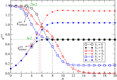
Figure 8: (Color online) The entanglement entropy $\varepsilon^{(n)}_{\rm planar}$ and $\varepsilon^{(n)}_{\rm vertical}$ with respect to the number of stacking $n$, at $h_{x}^{~{}}=0$ (circles), $h_{x}^{~{}}=h_{\rm c}^{~{}}$ (triangles), and $h_{x}^{~{}}=3$ (squares) for $D=2$, when $\Delta\tau=0.01$ and $h_{z}^{~{}}=0$.

We have thus defined $\varepsilon^{(n)}_{\rm planar}$ and $\varepsilon^{(n)}_{\rm vertical}$. Fig. 8 shows them with respect to $n$ at $h_{x}^{~{}}=0$, $h_{x}^{~{}}=h_{\rm c}^{~{}}$, and $h_{x}^{~{}}=3$. The tensor $T^{(0,0)}_{~{}}$ works almost as the identity which is applied to the vertical direction, and there is almost no correlation to the planar direction. For this reason, $\varepsilon^{(n)}_{\rm vertical}$ is close to $2\ln 2$, which corresponds to two completely entangled pairs, and $\varepsilon^{(n)}_{\rm planar}$ is very small. With increasing $n$, $\varepsilon^{(n)}_{\rm vertical}$ always decreases, while the planar one $\varepsilon^{(n)}_{\rm planar}$ increases. For $h_{x}^{~{}}=0$, both of the entropies are saturated to $\ln D=\ln 2$ at larger $n$ since the calculations are carried out with $D=2$.

When $\varepsilon^{(n)}_{\rm planar}$ and $\varepsilon^{(n)}_{\rm vertical}$ are close, it is possible to consider that $T^{(0,n)}_{~{}}$ is almost equally correlated with both the planar and the vertical directions, and this is the right situation to start the iterative processes in the HOTRG method. The vertical double-dot-dashed lines in Fig. 8 shows the value of such $n$. Within the typical range of the transverse field $0\leq h_{x}^{~{}}\leq 3$ we have used, the optimal number of the initial stacking lies in the interval $5\lesssim n\lesssim 8$. We have numerically confirmed that the HOTRG method, following Eqs. (13a)-(13c), can be performed in a stable manner after they have been started with $T^{(0,n\approx 6)}_{~{}}$.

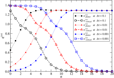
Figure 9: (Color online) The entanglement entropies at $h_{x}^{~{}}=h_{\rm c}^{~{}}$ for the three selected imaginary-time steps $\Delta\tau=0.1$ (circles), $\Delta\tau=0.01$ (triangles), and $\Delta\tau=0.001$ (squares).

The correct determination of $n$ also depends on the initial choice of $\Delta\tau$. Figure 9 shows both of the entropies at the critical field $h_{x}^{~{}}=h_{\rm c}^{~{}}$ for three selected imaginary-time steps $\Delta\tau$. As it is naturally understood, the smaller the $\Delta\tau$, the more initial iteration steps $n$ are necessary to satisfy $\varepsilon^{(n)}_{\rm planar}\approx\varepsilon^{(n)}_{\rm vertical}$. Although smaller $\Delta\tau$ lowers the Trotter-Suzuki error $(\Delta\tau)^{2}$, significantly more iterations are needed in the main HOTRG algorithm and round-off errors get accumulated for $\Delta\tau\ll 10^{-2}$, which negatively act against the improvement of numerical precision. Thus we have used $\Delta\tau$ of the order of $0.01$ for all the calculations in the main text.

References

- Gefen et al. (1984) Y. Gefen, A. Aharony, Y. Shapir, and B. B. Mandelbrot, J. Phys. A 17, 435 (1984).
- Luscombe and Desai (1985) J. H. Luscombe and R. C. Desai, Phys. Rev. B 32, 1614 (1985).
- Yi (2015) H. Yi, Phys. Rev. E 91, 012118 (2015).
- Kubica and Yoshida (2014) A. Kubica and B. Yoshida, arXiv:1402.0619 (2014).
- Yoshida and Kubica (2014) B. Yoshida and A. Kubica, arXiv:1404.6311 (2014).
- Wang et al. (2016) M. Wang, S.-J. Ran, T. Liu, Y. Zhao, Q.-R. Zheng, and G. Su, Eur. Phys. J. B 89, 27 (2016).
- Xu et al. (2017) Y.-L. Xu, X.-M. Kong, Z.-Q. Liu, and C.-C. Yin, Phys. Rev. A 95, 042327 (2017).
- Xie et al. (2012) Z. Y. Xie, J. Chen, M. P. Qin, J. W. Zhu, L. P. Yang, and T. Xiang, Phys. Rev. B 86, 045139 (2012).
- Genzor et al. (2016) J. Genzor, A. Gendiar, and T. Nishino, Phys. Rev. E 93, 012141 (2016).
- Wilson (1975) K. G. Wilson, Rev. Mod. Phys. 47, 773 (1975).
- Trotter (1959) H. F. Trotter, Proc. Amer. Math. Soc. 10, 545 (1959).
- Nishino et al. (2001) T. Nishino, Y. Hieida, K. Okunishi, N. Maeshima, Y. Akutsu, and A. Gendiar, Prog. Theor. Phys. 105, 409 (2001).
- Gendiar et al. (2003) A. Gendiar, N. Maeshima, and T. Nishino, Prog. Theor. Phys. 110, 691 (2003).
- Verstraete and Cirac (2004) F. Verstraete and J. I. Cirac, arXiv:cond-mat/0407066 (2004).
- de Lathauwer et al. (2000) L. de Lathauwer, B. de Moor, and J. Vandewalle, SIAM J. Matrix Anal. Appl. 21, 1523 (2000).
- Genzor et al. (2017) J. Genzor, T. Nishino, and A. Gendiar, Acta Phys. Slov. 67, 85 (2017).
- Feynman (1939) R. P. Feynman, Phys. Rev. 56, 340 (1939).
- Kolesik and Suzuki (1994) M. Kolesik and M. Suzuki, Physica A 215, 138 (1994).
- Amin et al. (2016) M. H. Amin, E. Andriyash, J. Rolfe, B. Kulchytskyy, and R. Melko, ArXiv e-prints (2016), eprint 1601.02036.
- Biamonte et al. (2017) J. Biamonte, P. Wittek, N. Pancotti, P. Rebentrost, N. Wiebe, and S. Lloyd, Nature 549, 195 (2017).
- Stoudenmire and Schwab (2016) E. M. Stoudenmire and D. J. Schwab, Advances in Neural Information Processing Systems 29, 479s (2016).
- Huggins et al. (2018) W. Huggins, P. Patel, K. B. Whaley, and E. M. Stoudenmire, arXiv:1803.11537 (2018).